An End-to-End Identification Algorithm for Smearing Star Image

Abstract

In the previous study, there were a few direct star identification (star-ID) algorithms for smearing star image. An end-to-end star-ID algorithm is proposed in this article, to directly identify the smearing image from star sensors with fast attitude maneuvering. Combined with convolutional neural networks and the self-attention mechanism of transformer encoder, the algorithm can effectively classify the smearing image and identify the star. Through feature extraction and position encoding, neural networks learn the position of stars to generate semantic information and realize the end-to-end identification for the smearing star image. The algorithm can also solve the problem of low identification rate due to smearing of long exposure time for images. A dataset of dynamic stars is analyzed and constructed based on multiple angular velocities. Experiment results show that, compared with representative algorithms, the identification rate of the proposed algorithm is improved at high angular velocities. When the three-axis angular velocity is 10°/s, the rate is still 60.4%. At the same time, the proposed algorithm has good robustness to position noise and magnitude noise.

1. Introduction

Star sensors are important high-precision attitude measurement devices, which are widely used in attitude determination for spacecraft [1]. However, the smearing star images, formed by sensors with high attitude angular velocity and long exposure time, pose huge challenges for star identification (star-ID) [2]. Star-ID is an important algorithm for star sensors to determine attitude. While a satellite is lost-in-space, the sensor will capture a star image in the field of view (FOV) and extract positions of stars through the process of denoising, thresholding, labeling and centroiding [3]. After this process, the star-ID algorithm is used to match the stars with the star database, to determine the attitude. As the technology of agile satellites develops, the improving maneuverability brings a wider range of applications. Rapid and exact determination of the attitude is critical to satellites. While the star sensors on satellites have high angular rates, there will be two problems with the star-ID algorithm. Firstly, due to a relatively long exposure time to the angular velocity, the star in the image inevitably changes from a stationary point to a line [4] so that the energy of the star is dispersed to multiple pixels, which means the brightness decreases. Algorithms of thresholding will not be able to distinguish stars from the background, resulting in missing stars. Secondly, due to the energy dispersal and the influence of noise, the centroid accuracy of the star point decreases seriously and brings positional noise to the stars. Both of the two problems will take extra time in the working process of the star sensor and bring difficulties to star-ID. An efficient star-ID algorithm is essential to the star sensor working in high angular velocity.

The traditional algorithms of star-ID mainly include two categories of subgraph isomorphism and pattern association [5]. The subgraph isomorphism algorithm is based on angular distance matching [6,7,8]. Based on the angular distance information between stars, these algorithms are the most common method to achieve accurate recognition by matching with the star catalog. However, such methods usually require precise positions of stars and parameters of the optical system for quicker searching [9,10]. Such methods usually require very precise optical parameters for the accuracy of the angular distance. In a dynamic situation, the identification rate will be affected due to the inaccuracy of the position. The grid algorithm is a representative of the application for pattern association in star-ID [11]. Seen as a pattern, the distribution of stars is used to identify by the features constructed artificially, such as radial and cyclic features [12] and log-polar transformation [13]. The star-ID algorithms based on patterns are less sensitive to star position or optical information, but robust to position errors. The algorithms usually require enough stars in the FOV, otherwise difficult to uniquely identify. However, due to the decrease in star energy in the image, the number of stars during the movement will be less than that in the static state. What is more, traditional algorithms based on patterns are usually constructed by intuition, easily insufficient for high-level features of star patterns. For smearing star images without sufficient number of stars, low-level features may not meet the discrimination degree of identification.

For the identification of smearing star images under dynamic conditions, some of the existing processing methods such as the improvement of pre-processing and the recovery of star energy. The local Kittler method [14], which is thresholding of preprocessing, was adopted in angular rates lower than 10°/s, but the method cannot completely extract the low-energy star point. Reference [15] proposes a denoising and signal enhancement method based on morphological methods. Reference [16] proposes a star-ID based on rolling shutter compensation robust to angular rates. However, they did not discuss extreme situations under high dynamics, which is the trend of agile satellite development. For star energy recovery, it is necessary to analyze the movement to get the degradation model [17]. Recovery usually requires inverse filtering, which takes extra time. The Radon transform and RL method are combined to estimate the motion kernel, which does not consider complex motion states [18]. The optimization method is adopted for blind restoration [19,20], but it takes a long time. For faster recovery, phase information of smearing is used for Wiener filtering [21], but the noise is not considered in the model. In addition, these algorithms have not discussed the robustness of star-ID under dynamic conditions.

The neural networks (NNs) give new solutions to star-ID in terms of high robustness. The star-ID algorithms using NNs are pattern-based, and the algorithms can output star index end-to-end from the image. The NNs not only extract deep pattern features to be more effective, but also have the same time complexity in different situations by saving the pattern library in the parameters [22]. In other words, it will not have different identification times due to different angular velocity, so as not to affect the determination of the attitude. Researchers have begun to use convolutional neural networks (CNNs) and back propagation neural networks in star-ID, which are robust to kinds of noise. However, the VGG16 model was used for the only static main star identification [23], and the model has too many parameters. The RPNet [24] and spider-web image for identification [25] require feature preprocessing to identify by artificially constructing patterns, which is difficult for smearing stars. These algorithms do not discuss the specific issues under motion conditions or consider the characteristics of dynamic stars.

In this paper, an improved NNs model architecture, aiming to deal with smearing star images, is proposed for dynamic star-ID. The proposed algorithm is an end-to-end identification of smearing images. With no need for thresholding or restoring stars, the algorithm directly identifies the smearing stars from the unprocessed images. The NNs model combines the feature extraction of CNNs and the Transformer encoder to identify. The Transformer is a new network for processing sequences. Based on the attention mechanism of the Transformer, the global characteristics of the dynamic features are introduced. The relative position characteristics between the stars in a FOV are emphasized by learning the spatial position. The learned characteristics are also abstracted into different semantic features to achieve more efficient encoding by adding semantic tokens. To test the validity of the model, the end-to-end algorithm is compared with two types of representative star-ID algorithms in different motion states. The robustness to different noise, position noise and magnitude noise that mainly affect smearing images, is tested under dynamic conditions.

The remainder of this paper is organized as follows. In Section 2, the principle of smearing stars in the images is clarified and how to construct the dataset is explained in detail. In Section 3, the model architecture and key feature processing of the algorithm are elaborated. In Section 4, the identification rate and robustness of the proposed algorithm in different motion states are compared with other algorithms. In Section 5, the experimental results are analyzed, and the reasons are given according to the principle of the algorithms. In Section 6, conclusions are given.

2. Datasets

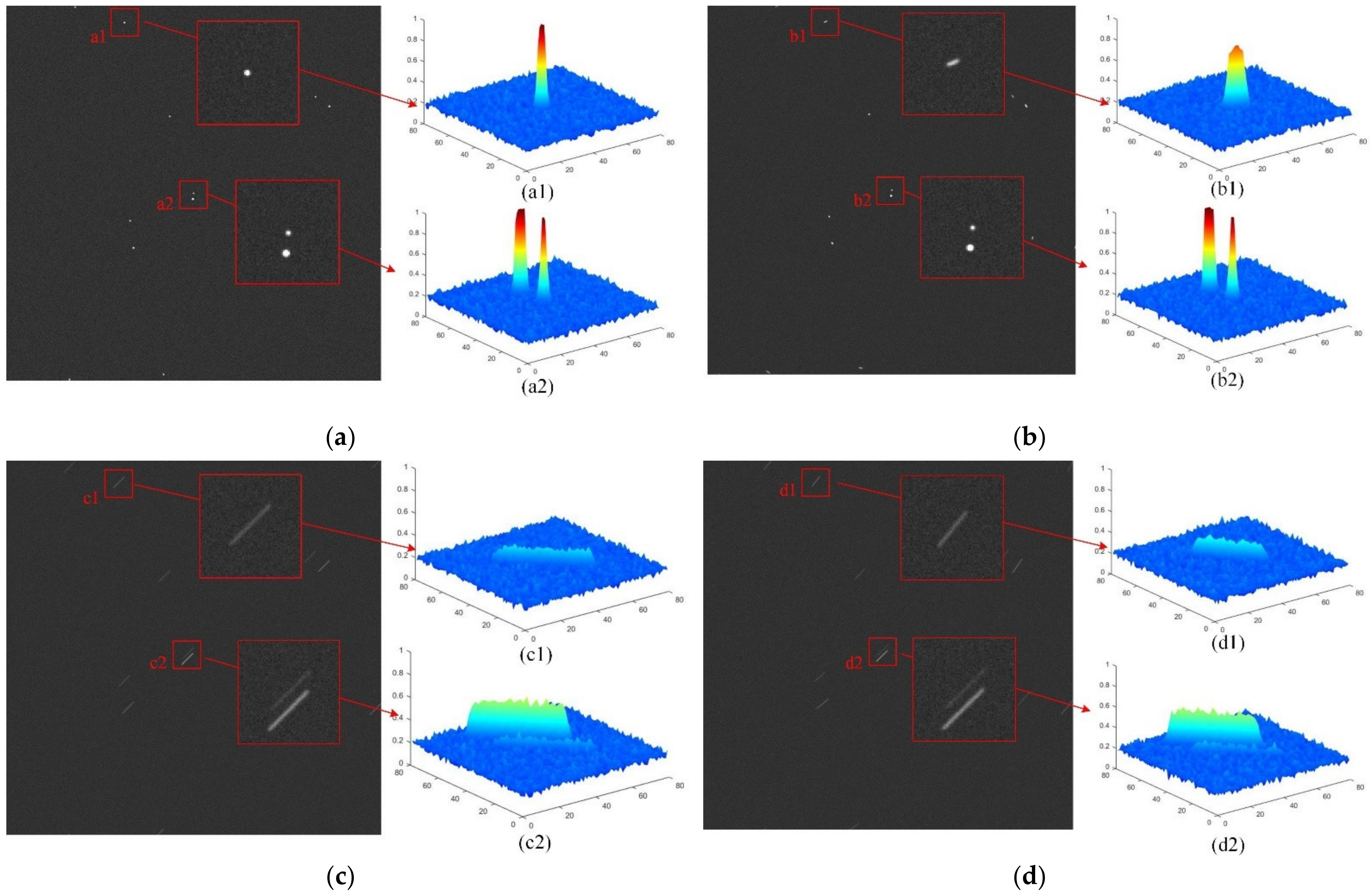
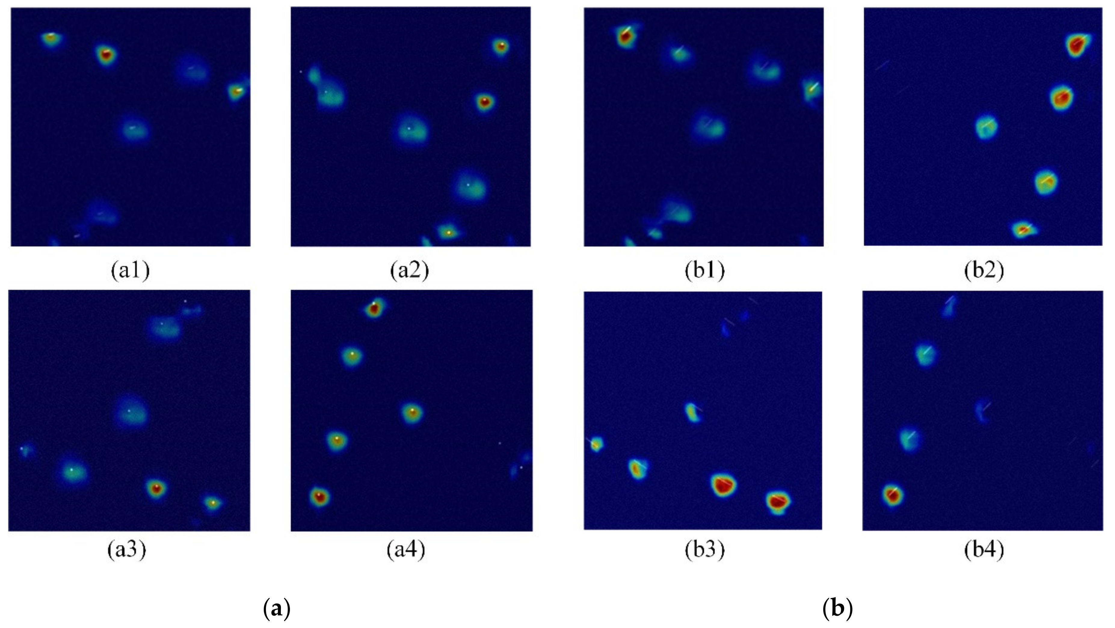
A star in the image taken by a star sensor under dynamic conditions usually has the phenomenon of smear. Figure 1 shows the comparison of star points in dynamic and static conditions. The 3D surface diagrams show the dispersion of the energy through the color of the heat maps. Different from the static image, the star point patterns in the dynamic state are diverse. At this time, the stars in the image will be mainly affected by the angular velocities.

The proposed end-to-end algorithm adopts the NNs theory, learns from the dynamic database and performs star-ID. Since the algorithm requires a large number of images for training but real data are difficult to obtain, the training data are supplemented by simulation. The proposed algorithm focuses on smearing star images at different angular velocities. It is necessary to complete the dataset according to the dynamic parameters of the star sensor. In this section, we will focus on the generation of star images and the principles of smearing star images, as well as the construction of data sets.

2.1. Principle of Smearing Star Images

In the research of star-id algorithm, the simulation generation of star images is the basis of algorithm testing. Forming a close-to-real star database according to the parameters can cut costs. Most situations can be generated through simulation without real occurrence. In this paper, the star image datasets are generated from the tycho-2 star catalog. Based on the optical system of star sensors, the simulation parameters of the detector are shown in

Table 1. Simulation parameters of the optical system.

Item	Quantity	Unit
Image plane dimension	1024 × 1024	pixel
Pixel size	0.012 × 0.012	mm
Instrument magnitude threshold	6	Mv
FOV	12 × 12	deg (°)
Focal length	58.5	mm
Radius of the point spread function	2	pixel
Exposure time	92	ms

. These parameters can ensure that the number of stars in the FOV meets the identification requirements for a unique pattern.

In the datasets, the stars above the instrument magnitude threshold of the sensor are named navigation stars. These stars are screened out from the star catalog, and the total number of navigation stars is 4331. The index number $i$ of each star is regarded as its corresponding category. In a star image, the star to identify is called the main star, and the other stars in the same FOV are called neighboring stars. The characteristics of the neighboring stars constitute the unique pattern of the main star. The navigation stars and main stars construct the pattern library by the same method. Matched with the pattern of the navigation stars, which are also composed of their neighboring stars, the main star in the image can be identified. The right ascension and declination $({\alpha }_i,{\delta }_i)$ of each navigation star $i$ in the celestial coordinate system are recorded for the generation of the images. In the process of constructing the datasets, the optical axis of the star sensor is set to the center position of each navigation star, so that the image can correspond to the main star.

According to the theory of star imaging [26], static and dynamic star images are both generated for training. Under static conditions, the distribution of star $i$ imaging chromatic speckles can be expressed by a two-dimensional Gaussian function, as $f_i(x,y)$ in Equation (1).

$$\begin{array}{l}I(m,n)={\displaystyle \underset{m,n}{\iint }{\displaystyle \sum _{i=1}^N{f}_i(x,y)}}dxdy+B\\ f_i(x,y)=\frac{1}{2\pi {\sigma }^2{E}^{M_i}}\exp \left[-\frac{{\left(x-x_i\right)}^2}{2{\sigma }^2}\right]\exp \left[-\frac{{\left(y-y_i\right)}^2}{2{\sigma }^2}\right]\end{array}$$

(1)

In the equation, $I(m,n)$ is the total number of photoelectrons on the $(m,n)$ pixel. The $x_i$ and $y_i$ are the center positions where the star projection transforms onto the image plane of the sensor. $M_i$ is the magnitude of the star. $N$ is the number of stars in the FOV. $E^{M_i}$ is the energy-gray coefficient, related to the apparent magnitude of the star $M_i$, the quantum efficiency, the integral time, and the optical system. $\sigma$ is the Gaussian radius which represents the energy concentration. $B$ represents background noise, which is affected by background brightness and sensor noise. In the simulation, the sensor noise is mainly composed of Gaussian noise and Poisson noise. Among the training and test dataset images, the background noise is simulated with Gaussian noise with variance 0.001. The simulated star image under static conditions is like Figure 1a.

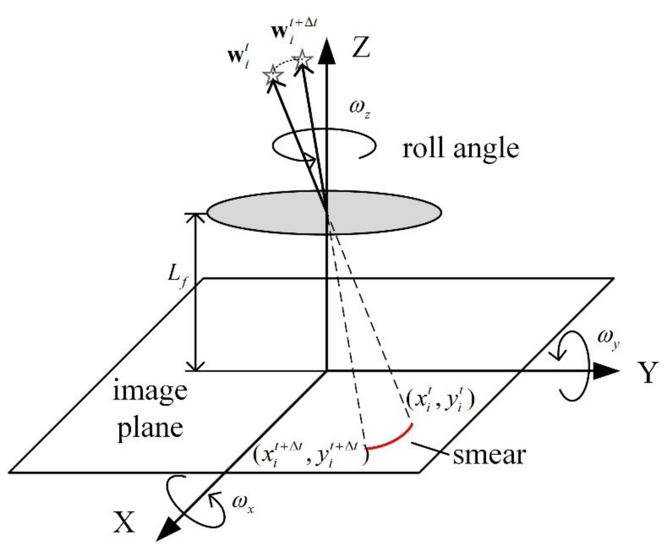
When the star sensor rotates at a high speed, due to the position change caused by the relative motion, the limited energy is dispersed to more pixels, and smearing star images are formed. Therefore, it is necessary to introduce the relationship between the position of the star on the image and the angular velocity of the star sensor. The coordinate system is shown in Figure 2. The direction vector of navigation star $i$ at time $t$ is $w_i^t$. The corresponding coordinates $(x_i^t, y_i^t)$ on the image plane are determined by the vector and focal length $L_f$ of the optical system. When the star sensor gets its attitude changed or moves with three-axis angular velocity $A^{t+\Delta t}$ from $t$ to $\Delta t$, the direction vector at the moment after the change is $w_i^{t+\Delta t}$, which can be expressed as Equation (2).

$$w_i^{t+\Delta t}=A^{t+\Delta t}{w}_i^t$$

(2)

Derived through the Taylor expansion of the angular velocity matrix $A^{t+\Delta t}$ and ignore higher-order terms due to the short exposure time, $A^{t+\Delta t}$ is simplified into (3), where $I$ is the identity matrix, and ${\omega }_x^t$, ${\omega }_y^t$ and ${\omega }_z^t$ represent the three axes angular velocities at time $t$.

$$A_t^{t+\Delta t}\approx I-\left[\begin{array}{ccc}0& -{\omega }_z^t& {\omega }_y^t\\ {\omega }_z^t& 0& -{\omega }_x^t\\ -{\omega }_y^t& {\omega }_x^t& 0\end{array}\right]\Delta t$$

(3)

So that the position of the star $(x_i^{t+\Delta t}, y_i^{t+\Delta t})$ on the image plane is determined by (4) after changing.

$$\left\{\begin{array}{c}{x}_i^{t+\Delta t}=x_i^t+(y_i^t{\omega }_z^t+L_f{\omega }_y^t)\Delta t\\ y_i^{t+\Delta t}=y_i^t-(x_i^t{\omega }_z^t+L_f{\omega }_x^t)\Delta t\end{array}\right.$$

(4)

Therefore, under dynamic conditions, Equation (1) is modified to (5), where $T$ is the exposure time.

$$\begin{array}{l}I(m,n)={\displaystyle \underset{m,n}{\iint }{\displaystyle \sum _{i=1}^N{g}_i(x,y)}}dxdy+B\\ g_i(x,y)={\displaystyle {\int }_0^{T}f\left[x-x_i(t),y-y_i(t)\right]}dt\\ ={\displaystyle {\int }_0^T\left(\frac{1}{2\pi {\sigma }^2{E}^{M_i}}\exp \left[-\frac{{\left(x-x_i(\Delta t)\right)}^2}{2{\sigma }^2}\right]\exp \left[-\frac{{\left(y-y_i(\Delta t)\right)}^2}{2{\sigma }^2}\right]\right)}d\Delta t\end{array}$$

(5)

Through the relationship between (4) and (5), the energy distribution of stars in the image can be calculated. The simulated star images under dynamic conditions are like Figure 1b–d. It can be seen that the stars in the same image have similar motion states and constant relative positions. The star image of Figure 1b is with roll angular velocity ${\omega }_z^t$ of 6°/s. Figure 1c has angular velocities on the X and Y coordinate axes, where $({\omega }_x^t,{\omega }_y^t,{\omega }_z^t)=(2,2,0)$ and the unit is °/s. Images in Figure 1d have three-axis angular velocities, $({\omega }_x^t,{\omega }_y^t,{\omega }_z^t)=(2,2,6)$. It can be found that the length of a star is mainly determined by ${\omega }_x^t$ and ${\omega }_y^t$, while ${\omega }_z^t$ affects its shape and has little effect on its length. In addition, the effect of the ${\omega }_z^t$ on the star in the center is less than the effect on the edges of the FOV. In view of this phenomenon, the setting of the roll angular velocity for training is relatively simple.

2.2. Training Dataset and Test Dataset

Since there is very little real data of the smearing star images, both the training and test dataset are generated by simulation. The target of generating the training dataset is to make the NNs model have stronger generalization ability, and the target of constructing the test dataset is to objectively evaluate the performance of the NNs. In this paper, the training set is constructed to improve the rotation invariance and the clustering ability of the algorithm. The rotation invariance means that when the roll angle of the star sensor changes, the pattern of the main star should not change. Star images of the same main star, with different angular velocities, should be clustered together so that the secondary features such as lengths and shapes of the smear do not affect identification.

In the star images, the roll angle ${\phi }_i$ is around the optical axis so that it changes the rotation angle of the image, as shown in Figure 3. The images are normalized to make them clearer, which is an important part of the NNs. To expand the dataset, as well as improve the rotation invariance, the roll angle of the star sensor is set to different angles. In the training set, the roll angle is set at 30° intervals to generate twelve different star images for the same main star. The training dataset is constructed based on sets of twelve images with different roll angles.

Smearing star images in different motion states are generated at $({\alpha }_i,{\delta }_i,{\phi }_i)$. Since the length of the star smear is not the main feature for identification, a larger velocity interval is used to prevent overfitting when constructing the training set. The overfitting here means that the training set covers the test set, making the test result invalid. The resultant angular velocity of ${\omega }_x^t$ and ${\omega }_y^t$ to be 2°/s, 4°/s, 6°/s, and 8°/s are selected respectively, and the directions are eight groups of 45° intervals, representing 8 smearing directions on the image. The angular velocity ${\omega }_z^t$ is selected to be 0° and ±6°, so that the resultant velocity of the three-axis angular velocities is constrained to be less than 10°/s. In this way, with 12 roll angles, 4 two-axis angular velocities, 8 smear directions, and 3 third-axis angular velocities, each set of static stars can be expanded to $12\times (1+4\times 8\times 3)=1164$ images. At the same time, to make the network more robust to real scenes and noise, one or two false stars and missing stars are randomly added to each star image to generate two new sets. So far, a main star has 3492 different scenes in the training dataset.

Different from the training dataset focusing on the dynamic characteristics, the test set pays more attention to the similarity with the real star images, ensuring the validity of the test results. Construct two test sets to test the algorithm. The test sets have two different movement situations. The construction method is to randomly select the directions of 2000 different main stars with random roll angles and generate smearing images with different resultant angular velocities at the main star positions. In the first test set, the ${\omega }_z^t$ is 0°/s and direction of ${\omega }_x^t$ and ${\omega }_y^t$ is arbitrary, which means that the resultant velocity is parallel to the image plane of the sensor. In the second test set, the three angular velocities are set to be completely equal to test the situation with three-axis attitude rotation, and the direction of the three velocities are arbitrary. Random Gaussian noise with a mean value of 0.25 and a variance of 0.001 was added to the background noise of the two test sets. At the same time, Poisson noise is added to simulate the situation of the sensor receiving electrons at the star point. In order to test the robustness of the algorithm, position noise and magnitude noise are added at the star point to the test dataset. These two kinds of noise represent the error of the star light in the measurement on the image. Both position noise and magnitude noise can be represented by Gaussian random noise and act on $(x_i^t, y_i^t)$ and $M_i$ of Equation (5), respectively.

3. Algorithm Description

In this section, an end-to-end star-ID algorithm for the smearing star images is proposed. The proposed star-ID algorithm, based on neural networks, is abstract into an image classification process. The main idea of the algorithm is the same as the pattern recognition star-ID algorithm. However, before recognition, the proposed algorithm does not require any preprocessing for the stars in the image. It does not perform thresholding, centroiding or star recovery, but directly identifies end-to-end output star index. Specifically, in the basic flow of the pattern recognition algorithm, the star closest to the center of the image is selected as the main star. After obtaining all the centroid position of the stars, it is usual to determine the unique pattern formed by the main star and neighboring stars. Then compare the pattern to the pattern library formed by navigation stars known in the star database to identify the main star. This identification mode that depends on the main star is regarded as the visual recognition of the main star. Differently, the preprocess of the proposed algorithm is to select a main star near the center of the FOV. The NNs calculate the features of the image centered on the main star and matches them with the pattern library. When building the pattern library of the main star, the NNs model regards its star index number as the category of the image. The model learns to form a star pattern autonomously and remembers the pattern feature in the parameters. Since the main star does not always appear in the center of the FOV and the constructed training database is based on FOV of 12°, the field of view of the star sensor should be at least 12°. The generated datasets satisfy most star sensors with a FOV greater than 12°. During the working process of a star sensor, it is easy to select a main star for identification if the FOV of star images is greater than training dataset.

The overall process of the proposed algorithm is shown in Figure 4. In addition to the construction of the dataset, it also includes feature extraction, feature encoding and classification, which form the NNs model.

3.1. Model Architecture

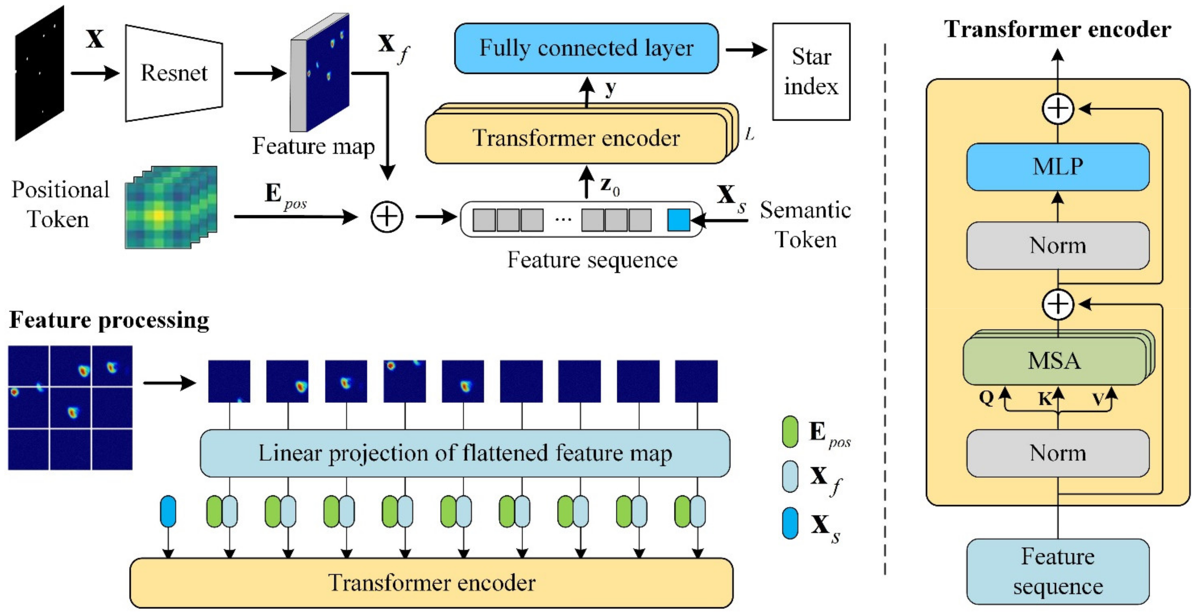
The specific architecture of the NNs model is shown in Figure 5. It mainly uses the theoretical calculation of spatial position coding in the Transformer and inherits its parallel structure and attention mechanism. The Transformer architecture is not sensitive to image features, so a feature extraction based on CNNs is necessary.

In the early stage of the model, star images are inputted through the feature extraction networks firstly, using the identity block of the residual neural network (Resnet) basic block for easier training [27]. Low-level features are generated by CNNs, aiming to learn the pattern at the densely distributed stars and the local features of motion. In the middle of the model, after getting the image feature map, positional tokens and semantic tokens are embedded into the feature for next learning, which will be introduced in part of Feature Processing. At the end of the model, the output feature sequences are sent to encoder of vision transformer [28], which is used to learn and associate more sparse distributions of star points. The Transformer encoder learns high-level semantic concepts from features. The classification is completed by encoded features and a fully connected layer so that the main star is identified.

3.2. Feature Extraction Networks

The feature extraction networks are composed of CNNs. When performing computer vision tasks, the CNN is usually used as the feature extraction layer. It can extract similar features located at different positions and increase the dimensionality of features. Among other star-ID networks, the convolution plays a major role. The features based on a single-layer CNN pay more attention to local features but lack the global receptive field and rotation invariance. For the images with sparse stars, the model needs to increase the size of the convolution kernel and the depth in order to connect distant features. Therefore, the learning of global image features requires a deep model such as VGG. However, part of the features extracted by deep CNNs will appear at the edge of the FOV, which reduces the application range when the direction of optical axis is shifted. In other words, when the main star shifts away from the center of the image, some features will also move out of the FOV. In addition, deep CNNs increase the complexity of the calculation and makes the model too large to be transformed into practical applications.

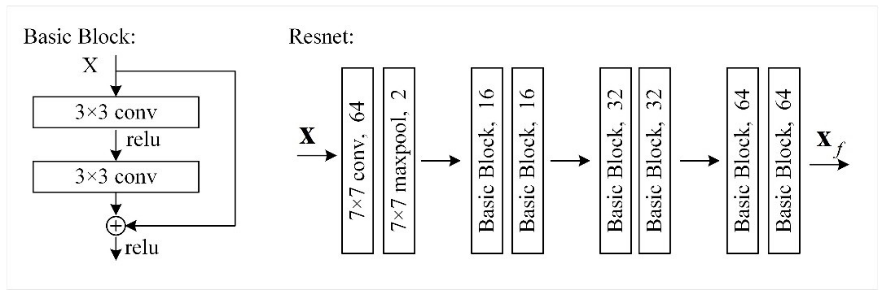
Therefore, in consideration of the defects of CNNs, the proposed networks only extract local features by CNNs, and the global features are provided by subsequent position encoding. As for the part of features appearing at the edge, the attention mechanism is to reduce the impact of shifting. In the feature extraction part, a more efficient and easy-to-train network, basic identity block of the Resnet, is selected to reduce the number of parameters. Resnet is an important improvement of convolutional neural networks. In this part of the model, the stride of the pooling layer in the Resnet is set to down-sample the feature map and reduce the total parameters. The cascaded CNNs gradually increases the feature dimension. Appropriate dimensional parameters are obtained through experimental tests. As shown in Figure 6, basic identity blocks are used to form feature extraction networks, which include 6 blocks composed of 12 convolutional layers, to complete the generation of local motion features. The parameters of the pooling layers are reset to adapt to the size of the subsequent encoder. Specifically, the down-sampling in the Resnet is performed by block1, block3, block5 and the Maxpool with a stride of 2. After four down-sampling, a feature map can be divided into 16 × 16 block features. The last layer of Resnet produces 64-dimensional feature maps. It provides a sufficiently deep feature sequence for subsequent encoding. Through the feature extraction networks, a star image $x$ generates a feature map $x_f\in {ℝ}^{D\times H\times W}$.

3.3. Feature Processing

After the feature map is generated, the feature processing can make the model have a stronger expressive ability, which is also necessary to adapt to the architecture of the Transformer Encoder. As the feature processing in Figure 5, the process includes flattening the map to sequences, embedding positional and semantic tokens. The processing makes it easier to encode the local features of stars to global features.

Firstly, as described above, convolutional layers are used to process some highly localized features. In order to learn more important global features, the model processes the feature map into sequences of finite length, and learns the stars features like the relationship between each word in a sentence.

And then, in the star images with few stars, the global features are more likely to appear in the deep space background. That is to say, what is learned is not at star points but background features, which is not in line with human intuition. The proposed model is more inclined to use relative position between stars, which is the foreground intuitively. In order to use the attention mechanism to position information, a similar position encoding method of Vision Transformer is introduced [28]. Differently, in the proposed model, position encoding uses learnable parameters instead of artificial coding. The flattened sequences learn star features by embedding the positional tokens.

In addition, the semantic concept of star images is introduced to identify stars. This concept is like constellation information, so that the information composed of stars has a better expression. In the process of feature sequence, a learnable semantic token is embedded. The model can use the token to learn the star category after encoding.

The process can be expressed as (6). The last two dimensions of the feature map are flattened to obtain a feature sequence of length $N$, where $N=H\times W$. The learnable positional token $E_{pos}$ is embedded to the flattened feature map $x_f^N$. Similarly, the learnable semantic token $x_s$ is embedded in the position-encoded feature map to obtain a feature sequence $z_0$. The feature sequence is input to the encoder to learn features at different positions.

$$z_0=\left[x_s, x_f^N+E_{pos}\right],z_0\in {ℝ}^{D\times \left(N+1\right)}$$

(6)

3.4. Transformer Encoder

The Transformer has excellent performance of parallel processing sequence and is widely used in natural language processing because of its attention to the position of words in the sentence. Similarly in star-ID, the position relationship between the main star and neighboring stars needs to be paid attention to. Transformer encoders with multi-head self-attention (MSA) are therefore introduced into the networks. The MSA is an attention mechanism relating multiple positions of elements to compute a representation of the sequence [29]. The basic structure of MSA is self-attention (SA) as in (7). In the model, SA is to realize the association between stars in sequence. The calculation of SA is as (8) and (9). The relationship between the elements in the sequence is calculated by three important matrices, queries $Q$, keys $K$, values $V$, and $Q,K,V\in {ℝ}^{D\times \left(N+1\right)}$. According to the theory of Transformer, queries and keys are used to match the proximity between each element and other elements in the feature sequence. The values of each element are combined, considering the whole sequence to achieve attention to the global feature. In the formulas, $W_{qkv}$ and $W_{msa}$ are learnable parameter matrices and $k$ is called the number of heads.

$$\mathrm{MSA}(z)=W_{msa}[{\mathrm{SA}}_1(z);{\mathrm{SA}}_2(z);\cdots ;{\mathrm{SA}}_k(z)],W_{msa}\in {ℝ}^{D\times kD}$$

(7)

$$[Q;K;V]=W_{qkv}z,W_{qkv}\in {ℝ}^{3D\times D}$$

(8)

$$\mathrm{SA}(z)=V\cdot \mathrm{softmax}(K^{\mathrm{T}}Q)$$

(9)

The right part of Figure 5 is a single layer of the Transformer encoder. The MLP blocks and Layer norm (LN) are applied in the encoder, and they are used to implement sequence encoding to reduce the redundancy of representation. The specific calculations of MSA and MLP are as (10), where $L$ is the depths of the encoder. In the last layer of the encoder, the output $y$ is represented as the encoded semantic token $z_L^0$ as in (11). Since $z_L^0$ is a learnable vector, when it is used for classification, it has different semantic information. $z_L^0$ is encoded with other features in the sequences, so that it can also encode the position of stars. Finally, a fully connected layer is used to create a connection between semantics and star index.

$$\begin{array}{l}z{\prime }_l=\mathrm{MSA}\left(\mathrm{LN}\left(z_{l-1}\right)\right)+z_{l-1},l=1\cdots L\\ z_l=\mathrm{MLP}\left(\mathrm{LN}\left(z{\prime }_l\right)\right)+z{\prime }_l,l=1\cdots L\end{array}$$

(10)

$$y=\mathrm{LN}\left(z_L^0\right)$$

(11)

So far, the NNs directly output star index from the smearing image. The proposed end-to-end algorithm focuses on the identification based on the position of the stars. According to the analysis of smearing star images, the relative position of the stars will not change significantly in an image, no matter how the star sensor is maneuvered. In other words, the motion feature and the position feature are separated. Correspondingly, the proposed model clusters different motion states by learning local features and classifies by learning global features. The Resnet generates local feature maps that are divided into feature blocks. The encoder associates the position between feature blocks and records semantic features. In this way, the identification will not be interfered by motion, and the networks will learn less from the edge or background of the image. Pay more attention to star points to make the star-ID performance better.

4. Experiment

The NNs are built based on the Pytorch framework, and the training is performed on 3.4-GHz desktop computers. The strategy of training does not consider robustness at first, and inputs part of the training set without false stars and missing stars into the network. Then, based on this pre-training, a full dataset is trained to increase the robustness of the model. During training, the image is first reshaped to 256 × 256, and then normalized with a mean and variance of 0.1. The encoder sets 6 heads to focus on 6 different degrees of global information, and its depth is set to 8. Set the batch size to 160 and use the Adam optimizer for optimization.

The following experiments are carried out on the CPU. The average identification time of the proposed algorithm for each 1024 × 1024 image is 56.5 ms. Compared with the traditional algorithm, the identification time has increased. However, due to the end-to-end characteristics, no recovery method is required. It is known that the restoration time for a 1024 × 1024 image is on the order of 1 s [20]. The proposed algorithm achieves a significant reduction in time while ensuring the identification rate. In terms of storage, the size of the model is 47.1 MB, which is significantly smaller than the 537.5 MB of VGG16 model.

4.1. Identification Rate in Dynamic States

To test the performance of the algorithm under dynamic conditions, smearing star images of two kinds of motion states in the test datasets are simulated. The simulation method is as described in Section 2 on the test datasets. The image used in this section does not include the position noise and magnitude noise of the star. Since there are few algorithms for smearing star-ID, two traditional types of representative algorithms are selected to compare the performance of the proposed algorithm. The grid algorithm based on pattern association and the triangle algorithm based on angular distance are tested to compare. The star point extraction process of these two algorithms adopts the same method [3], while the proposed algorithm does not need the process. The FOV of all algorithms is 12°. A successful identification refers to the correct output of the main star index and does not include the identification of the neighboring stars in the FOV. 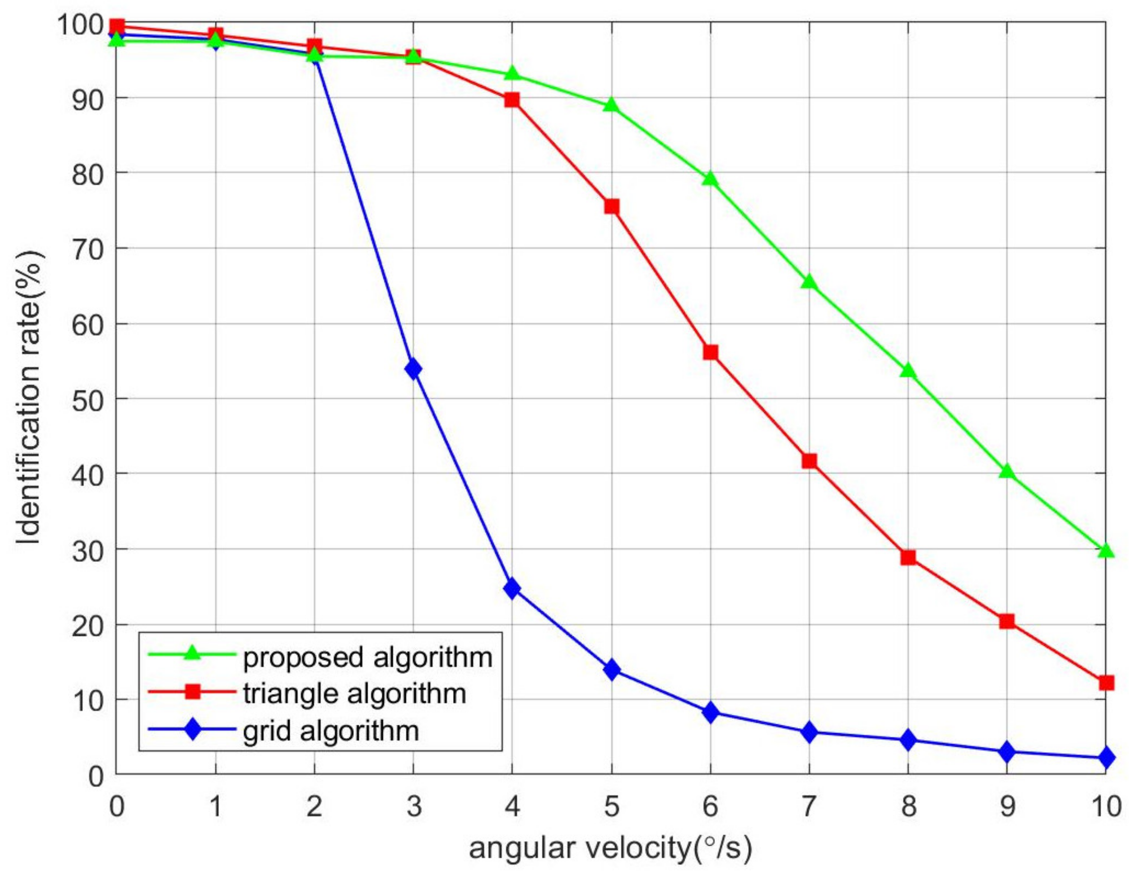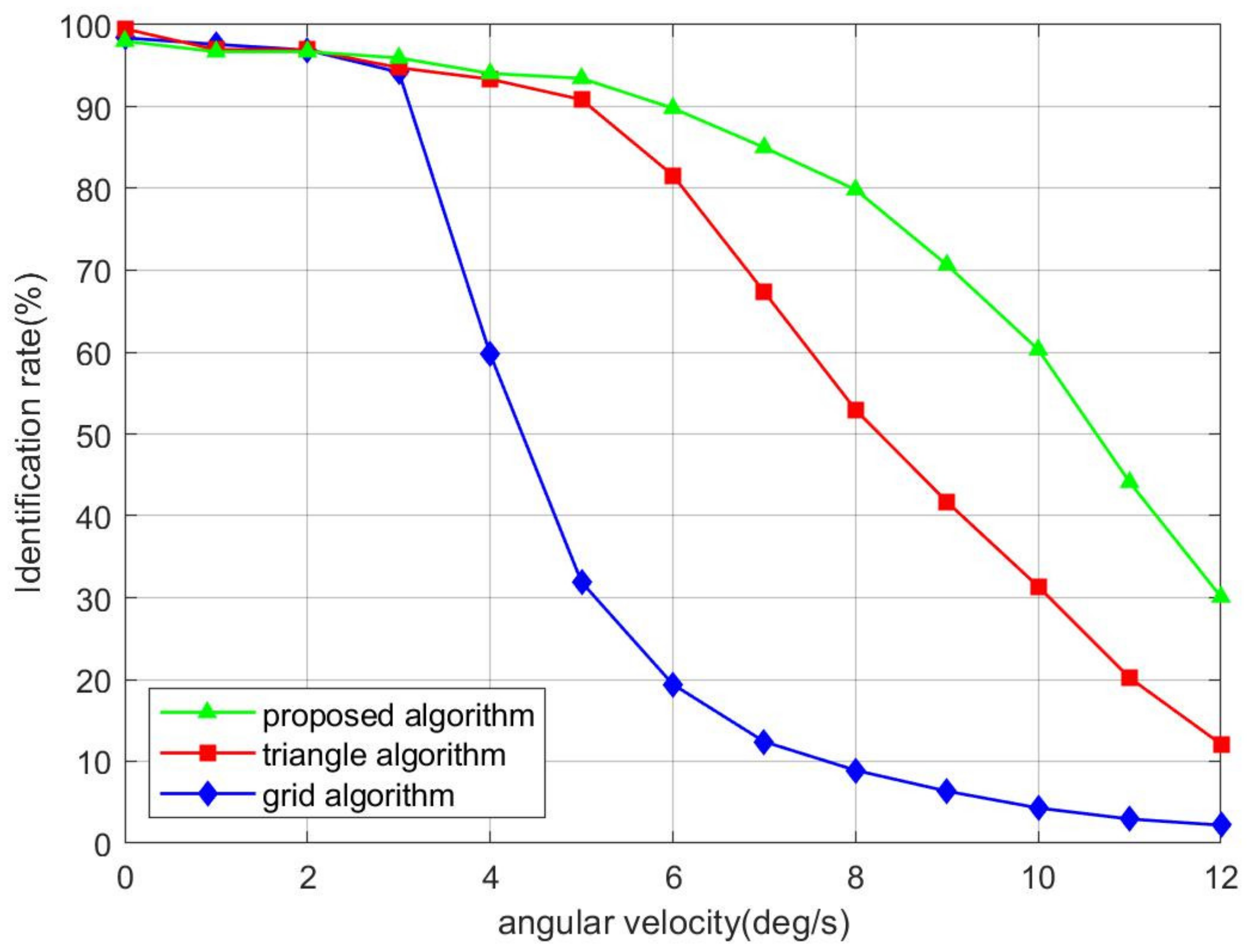The experimental results are shown in Figure 7 and Figure 8.

Figure 7 corresponds to the test result with only two-axis angular velocity motion, corresponding to ${\omega }_x^t$ and ${\omega }_y^t$ in the coordinate system. That is to say, the direction of angular velocity is parallel to the image plane. The angular velocity has the greatest impact on the image at this time. The resultant angular velocity of the test ranges from 0°/s. to 10°/s. When the velocity is higher, there are almost no star points on the image. Each angular velocity has 2000 images, and the two velocities direction with the roll angle are random. The results show that with the increase in the resultant velocity, the identification rates of the three algorithms all decrease. The grid algorithm is the first to be affected and begins to drop sharply when the angular velocity is greater than 2°/s. The rate drops from 98.2 to 1.95% when the angular velocity increases from 0°/s to 10°/s. The identification rate of the triangle algorithm drops from 99.3 to 12.15%. The accuracy of the proposed algorithm changes slowly with the increase in angular velocity. The identification rate drops from 97.5 to 29.5%. When the resultant velocity is greater than 4°/s, the identification rate of the proposed algorithm is higher than the other two algorithms.

The test dataset corresponding to Figure 8 has three-axis angular velocities. The resultant angular velocity of the test ranges from 0°/s. to 12°/s. The numerical values of the three-axis velocities are equal, and the directions are random, to get the result of a more general three-axis maneuver. For the three algorithms compared, the experimental results are roughly the same as the first test dataset. The identification rate of the triangle algorithm drops from 99.3 to 12.1% and the grid algorithm drops from 98.4 to 2.2 %. The identification rate of the proposed algorithm drops from 97.9 to 30.1%. It has the highest rate at the same angular velocity and realizes the improvement of star-ID for smearing images.

4.2. Robustness Experiment

The two kinds of noise, position noise and magnitude noise, are tested in this section to verify the robustness of the star-ID algorithms. These two kinds of noise represent the impact on the star point characteristics at the image level. Among them, the position noise refers to the error of the position measurement on the image plane of the optic system. The magnitude noise refers to the error of the brightness of the star by the star sensor measurement. Both the error distributions can be considered mainly as Gaussian. For position noise, after determining the smearing trace of stars, a random error of the position is added to $(x_i^{t+\Delta t}, y_i^{t+\Delta t})$ in Equation (5) to simulate the uncertainty of the position measurement. For magnitude noise, the random error is added to $M_i$.

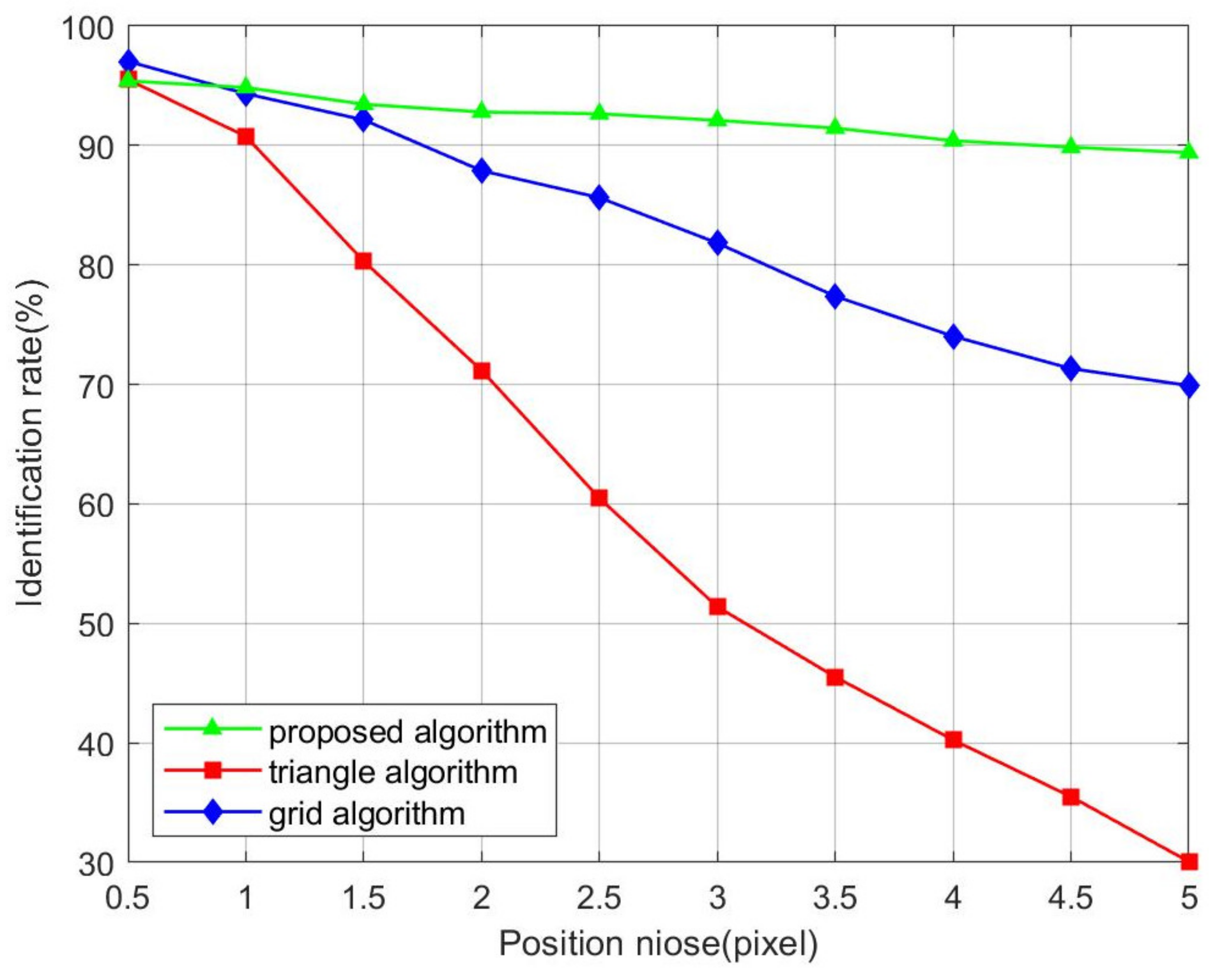
Specifically, the position noise with different standard deviations is added to the star centroid locations for each image at an angular velocity of 0°/s to simulate the star position error. In the test, the standard deviation of position noise ranges from 0.5 to 5 pixels, and 2000 images are selected for each position noise. Figure 9 illustrates the influence of position noise on the identification rate of different algorithms. The identification rates of triangle and grid algorithms have decreased to varying degrees. The identification rate of the triangle algorithm drops from 95.4 to 30.6%, and the rate of the grid algorithm from 97.1 to 69.9%, when the standard deviation of position noise increases. Unlike the two algorithms tested, the proposed algorithm is more robust to positional noise. The rate of the algorithm decreases slightly and remains above 89%. When there are two-axis angular velocities, the influence of position noise on the identification rate is shown in

Table 2. Identification rate of different position noise.

Angular Velocity	Algorithm	Position Noise (Pixel)
		1	2	3	4	5
1°/s	A	94.3%	93.1%	91.9%	89.2%	88.7%
	B	92.5%	70.7%	55.0%	41.4%	30.2%
	C	88.4%	83.6%	76.8%	71.9%	67.0%
3°/s	A	90.3%	88.5%	87.7%	85.4%	83.1%
	B	88.7%	68.1%	46.1%	30.7%	21.0%
	C	40.4%	40.3%	38.9%	36.0%	35.5%
5°/s	A	84.9%	81.5%	79.7%	76.5%	73.1%
	B	70.2%	60.7%	32.6%	15.5%	10.5%
	C	15.5%	13.1%	11.0%	7.2%	7.05%
7°/s	A	59.7%	55.2%	50.5%	46.3%	39.1%
	B	31.7%	18.7%	10.6%	7.8%	4.1%
	C	5.45%	5.1%	4.15%	3.75%	5.5%

. In the table, A, B and C represent the proposed end-to-end algorithm, triangle algorithm and grid algorithm, respectively. The numbers in bold indicate the best rate among the three algorithms under the same conditions. It can be found that the proposed algorithm has a better robustness to position noise.

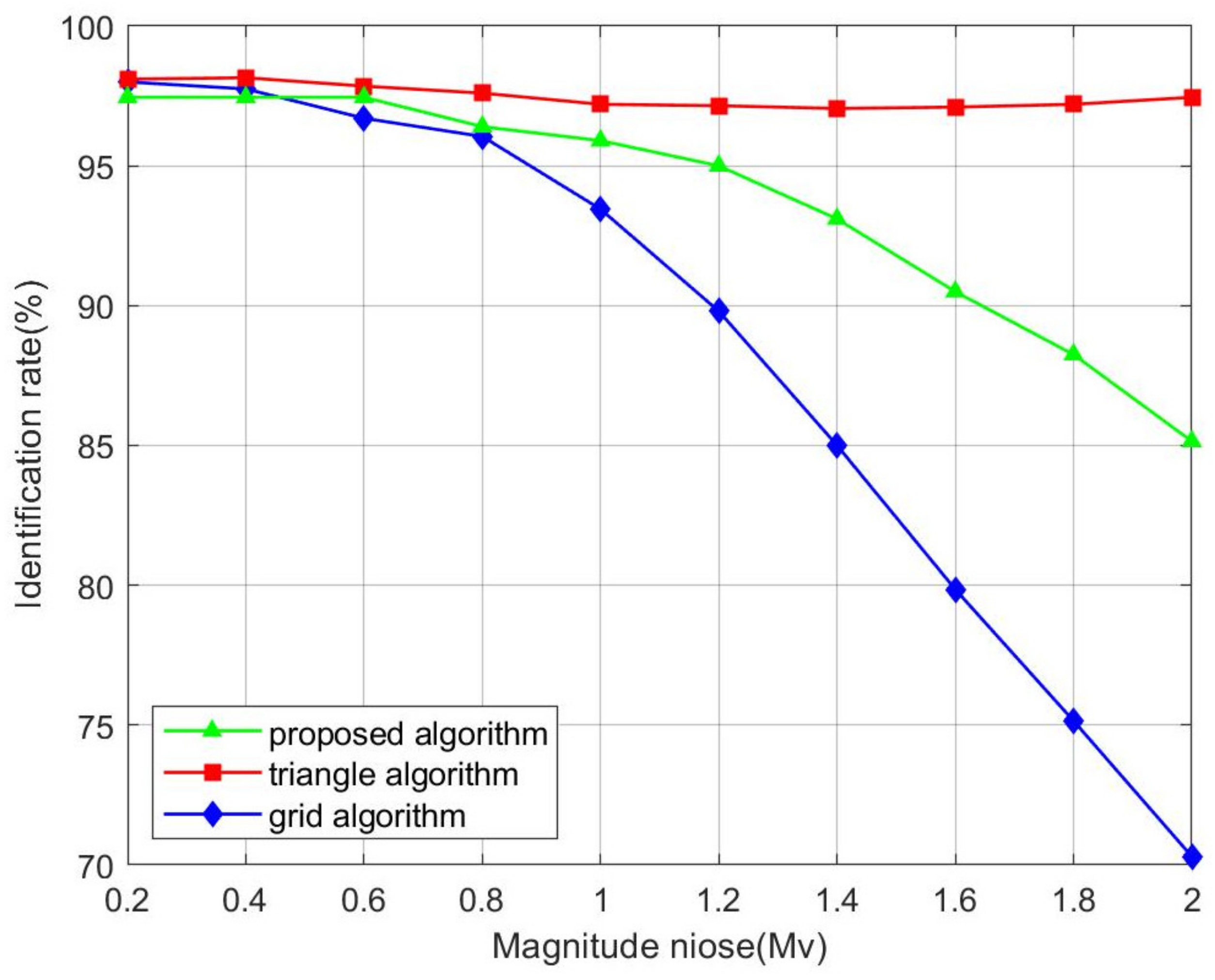
The magnitudes of stars are added with Gaussian random noise with different standard deviations to test the effect of the star magnitude error. The standard deviation ranges from 0.2 Mv to 2 Mv, and 2000 images are selected for each kind of magnitude noise. Figure 10 illustrates the influence of magnitude noise on the identification rate of different algorithms. The rate of the triangle algorithm is maintained at about 98%, which reflects the characteristics of star-ID based on angular distance. As a pattern recognition algorithm, the rate of the grid algorithm dropped from 98.1 to 70.3% due to missing stars caused by noise. The identification rate of the proposed algorithm decreases to 85.1% with the increase in magnitude noise. However, compared with grid algorithm, this algorithm has a higher identification rate under the same standard deviation of the magnitude noise. When there are two-axis angular velocities, the influence of magnitude noise on the identification rate is shown in

Table 3. Identification rate of different magnitude noise.

Angular Velocity	Algorithm	Magnitude Noise (Mv)
		0.2	0.4	0.6	0.8	1
1°/s	A	96.8%	96.1%	95.7%	95.5%	95.1%
	B	97.3%	96.6%	97.0%	96.9%	97.4%
	C	75.8%	67.8%	56.3%	53.3%	49.9%
3°/s	A	91.2%	90.1%	89.5%	88.4%	87.1%
	B	91.4%	90.7%	89.1%	87.3%	86.9%
	C	38.2%	37.3%	36.8%	30.2%	25.5%
5°/s	A	85.3%	83.6%	75.4%	68.2%	57.5%
	B	71.4%	67.7%	62.5%	55.3%	51.0%
	C	14.3%	13.7%	11.5%	10.2%	7.05%
7°/s	A	60.9%	57.3%	51.8%	42.7%	29.5%
	B	35.9%	33.6%	31.6%	27.8%	21.1%
	C	5.45%	5.5%	5.15%	4.85%	4.3%

. The standard deviation of magnitude noise in the table ranges from 0.2 Mv to 1 Mv, which is more in line with the measurement error of the star sensor. It can be found that the proposed algorithm is more robust to magnitude noise under high dynamic conditions.

5. Discussion

5.1. Analysis of Results

From the experiments on the two test datasets in Section 4.1, we can see the identification rates of the three algorithms all decrease but the rate of the proposed algorithm is higher than the other two algorithms under high dynamic conditions. The reason is that as the speed increases, the star energy is dispersed so that some stars disappear in the field of view. The identification rate of the triangle algorithm drops because the algorithm uses the angular distance between stars for matching, and the accuracy of star point extraction under dynamic conditions has a great impact on the result. The proposed algorithm and the grid algorithm belong to the same type of pattern recognition. The disappearance of the star caused the wrong pattern to be identified. The grid algorithm is severely affected and drops sharply under high dynamic conditions. This is because the increase in the length of the star has caused a major change in the grid where the star center is located, and a wrong pattern has been generated. The accuracy of our end-to-end algorithm changes slowly with the increase in angular velocity. Because the algorithm does not segment the image to generate features, like the grid, but encodes star positions to identify. This makes the algorithm more robust to position deviation. The position of dark stars will also be found thanks to the attention mechanism. This makes the algorithm improve the identification rate under dynamic conditions.

From the results of Figure 7 and Figure 8, it can also be found that the z-axis angular velocity has a relatively low impact on the identification rate. Since this angular velocity has little effect on the length of smearing, which can be equivalent to the change of other angular velocities, the velocities parallel to the image plane are mainly responsible for the decrease in recognition rate. In the two results, the corresponding relationship between the three-axis angular velocity components and the two-axis angular velocities can be found. Based on this analysis, two-axis angular velocities are used for robustness experiments.

In the robustness experiment, the results show that the proposed algorithm is best robust to position noise. As the position noise increases, the identification rates of the other two algorithms decrease. The triangle algorithm based on angular distance is most affected, while the grid algorithm based on pattern is relatively robust to position noise. This also verifies the advantages of pattern recognition star-ID algorithms. As the angular velocity increases, the trend still exists. The robustness of the proposed algorithm is still relatively better. For magnitude noise at static, the triangle algorithm has the best robustness because it does not depend on magnitude information. The proposed algorithm has some improvements over the grid algorithm. The robustness to magnitude noise has the same trend at low angular velocity. However, when the angular velocity is large, the identification rate of the proposed algorithm is higher. This is because as the speed increases, the star energy is dispersed. This influence, which makes the angular distance error larger, exceeds the influence of magnitude noise. At this time, the proposed algorithm is better than the triangle algorithm.

5.2. Visual Analysis of Features

In order to clearly understand the features learned in the extraction part and increase the interpretability of the networks, we use feature visualization technology to display. The specific method is to connect the sensitive area feature extraction networks to the Grad-CAM [30], which displays features by calculating the gradient of feature weights. As shown in Figure 11, the feature maps generated by Resnet are marked with heat maps. The red part represents the key recognized position, and the blue part is the relatively insensitive position.

The figure shows the relationship between different roll angles and different motions of the same main star. It can be found that the features displayed by the heat map are concentrated around the star points, and only local information is extracted. It can be found that the features displayed by the heat maps are concentrated around the star points, and only local information is extracted. From the perspective of global features, star maps with different motion states extract features at the same location and are not disturbed by smearing star. When the identified star images are rotated, the highly recognized feature part rotates by the same angle, and the relative position remains unchanged. That is to say, the learned features have rotation invariance to the distribution of stars. We think this is a form based on relative position and has semantic features similar to constellation information.

6. Conclusions

An end-to-end star-ID algorithm based on neural networks for smearing star images is proposed in this paper. The algorithm simplifies the identification process and can help to deal with the problem of long time and poor robustness of star-ID, in the case of high angular velocity attitude maneuvers of star sensors. The networks can efficiently realize the main star-ID by extracting different features and focusing on learning the relative position information between stars. The accuracy and robustness of the algorithm are tested emphatically, while considering the size of the model and the recognition time. The experimental results show that under dynamic conditions, the algorithm has a great improvement in the recognition rate. When the three-axis angular velocity is greater than 5°/s and less than 10°/s, the recognition rate of the proposed algorithm is above 60%. It also has strong robustness to positional noise. Although the robustness to magnitude noise is relatively weak, it has a greater improvement compared to the grid algorithm.