Ice Sheet Topography from a New CryoSat-2 SARIn Processing Chain, and Assessment by Comparison to ICESat-2 over Antarctica

Abstract

In this study, we present a new level-2 processing chain dedicated to the CryoSat-2 Synthetic Aperture Radar Interferometric (SARIn) measurements acquired over ice sheets. Compared to the ESA ground segment processor, it includes revised methods to detect waveform leading edges and perform retracking at the Point of Closest Approach (POCA). CryoSat-2 SARIn mode surface height measurements retrieved from the newly developed processing chain are compared to ICESat-2 surface height measurements extracted from the ATL06 product. About 250,000 space–time nearly coincident observations are identified and examined over the Antarctic ice sheet, and over a one-year period. On average, the median elevation bias between both missions is about −18 cm, with CryoSat-2 underestimating the surface topography compared to ICESat-2. The Median Absolute Deviation (MAD) between CryoSat-2 and ICESat-2 elevation estimates is 46.5 cm. These performances were compared to those obtained with CryoSat-2 SARIn mode elevations from the ESA PDGS level-2 products (ICE Baseline-D processor). The MAD between CryoSat-2 and ICESat-2 elevation estimates is significantly reduced with the new processing developed, by about 42%. The improvement is more substantial over areas closer to the coast, where the topography is more complex and surface slope increases. In terms of perspectives, the impacts of surface roughness and volume scattering on the SARIn mode waveforms have to be further investigated. This is crucial to understand geographical variations of the elevation bias between CryoSat-2 and ICESat-2 and continue enhancing the SARIn mode level-2 processing.

1. Introduction

Monitoring the continental ice sheet is a crucial issue to understand and evaluate the impacts of global warming. In this context, the polar ice sheet melting needs to be thoroughly surveyed as it dominates uncertainties in the projected sea level [1]. Mainly thanks to its near-global coverage and periodic revisit, satellite remote sensing has substantially improved our understanding of the ice sheet dynamics over the last decades. Among the different techniques employed, spatial altimetry is a powerful tool to monitor the ice sheet mass balance by measuring the ice topography, and converting its evolution in time into mass change. Since the early 1990s, spatial altimetry has provided a continuous time series on mass change rate, mostly composed of data acquired in the conventional Low Resolution Mode (LRM) from ERS 1 and 2, ENVISAT, and, more recently, CryoSat-2 and SARAL [2,3].

Launched in 2010 by the European Space Agency (ESA), CryoSat-2 is the first satellite mission carrying a pulse-limited radar altimeter with Synthetic Aperture Radar (SAR) capabilities [4]. As implemented in the CryoSat-2 Payload Data Ground Segment (PDGS), the unfocused SAR processing dramatically reduces the along-track footprint, from several kilometers to ~300 m compared to LRM [5]. In addition, when activated, the second antenna of CryoSat-2 enables a SAR Interferometric Mode (SARInM) processing to geolocate the radar returns within the SAR mode footprint over sloping surfaces [6]. CryoSat-2 operates in SARInM according to a geographical mask, including the polar ice sheets margins. Compared to LRM and SAR mode, several studies demonstrated the SARInM added value over these areas [7,8], challenging for spatial radar altimeters due to the topography variations at the footprint scale.

In 2003, The National Aeronautics and Space Administration (NASA) launched the Ice, Cloud, and land Elevation Satellite (ICESat), the first spaceborne laser altimetry mission specifically designed to measure changes in polar ice [9]. Despite laser lifetime issues, the mission was successful, notably by providing updated estimations of the polar ice sheets’ mass balance. Launched in September 2018, ICESat-2 is a follow-up to the ICESat mission and brings several technical enhancements. A denser surface sampling is achieved thanks to the addition of left/right across-track beams. Moreover, the footprint size and along-track spacing are smaller to optimize elevation retrievals over heterogeneous glaciers [10]. ICESat-2 ATL06 elevations over the Antarctic ice sheet interior have a reported accuracy and precision, respectively, of about 3 cm and 7 cm [11]. Hence, ICESat-2 is capable of providing a reliable calibration reference of the ice sheet topography at the snow-air interface. In contrast, spatial radar altimetry does not reach this level of performance over ice sheet. Nevertheless, the measurement accuracy and precision are constantly being improved, thanks to the technical innovations made on the altimeters, and the upgrade of ground segment data processing. Concomitant acquisitions of laser and radar altimeters over ice sheet are thus highly beneficial to evaluate the performances of radar altimeters, and quantify the potential added value of new radar data processing.

In Section 2 of this paper, we present a newly developed level-2 processing chain to derive surface topography from CryoSat-2 SARInM level-1b products and referenced as the “CLS processing” in the following text. An initial evaluation of this processing chain is performed over the Austfonna ice cap, Svalbard, thanks to the CryoSat-2 SARInM benchmark furnished by Sandberg Sørensen et al. [12]. In Section 3, CryoSat-2 SARInM and ICESat-2 ATL06 elevations are compared over the Antarctic ice sheet. This analysis is performed using CryoSat-2 estimations from the CLS and the PDGS ICE Baseline D processors. The results are discussed in Section 4, and investigations are proposed to further understand and improve the SARInM altimetry over ice sheet.

2. Ice Sheet Topography from CryoSat-2 SARInM Data

2.1. SARInM Level-1 and Level-2 Processing Description

In practice, over diffuse reflecting surfaces, the topography measured by radar altimeters is estimated at the point where the satellite–surface distance is the shortest: the so-called Point Of Closest Approach (POCA). Over a flat area, this point is located at nadir, but is shifted in case of a tilted surface or an irregular relief [13]. In LRM and SAR mode altimetry, an a priori knowledge of the topography is necessary to locate the POCA position. The accuracy and precision of the estimated elevation, therefore, rely on the accuracy of the employed Digital Elevation Model (DEM). Geolocation errors are diminished in unfocused SAR mode compared to LRM, due to the reduced along-track footprint [14,15]. In fact, the POCA remains located within the Doppler band footprint and is therefore not, or weakly, sensitive to along-track topographic variations. The SARIn technology was developed to optimize the radar measure over steeply sloping surfaces, by providing the capability to geolocate the radar returns within the Doppler band footprint.

When CryoSat-2 operates in SARInM, the second satellite antenna is activated to receive the pulses emitted by the first antenna. The pulses measured by the two antennas are processed in two parallel chains in the ground segment. At level-1b, an unfocused SAR processing is performed, discriminating the surface sampled on Doppler bands of about 300 m width. From different satellite positions along the orbit, a same Doppler band can be sampled at different look angles to generate a delay/Doppler stack. The stacked signals are multi-looked (i.e., summed) to generate the SAR waveform. The SARInM waveform corresponds to the average of the two SAR waveforms derived from each antenna. A complex cross-product calculation between the two SAR measurements produces the interferometric phase difference and coherence signals. This information allows locating the radar returns within the SAR mode footprint. More details about unfocused SARInM can be found in Jensen et al. [16] and Wingham et al. [4]. Cullen et al. [17] supplied a description of the CryoSat-2 level-0 to level-1b processing architecture.

In radar altimetry, the main objective of the level-2 processing is to derive the surface topography from the waveforms generated at level-1. In contrast to ocean acquisitions, the waveforms measured over the continental ice sheets have diverse shapes. This is the result of topography variations within the footprint and the complex interaction between the Ku band radar-wave signal and the snow medium. Hence, several geophysical parameters act on the waveform shape: the surface roughness (from centimeter to kilometer scales) and several snow parameters, mainly: density, grain size, temperature, snowpack stratification [18]. Over ocean, physical models of the radar signal have been established to characterize the waveforms measured by the altimeter [19]. With these models, the geophysical parameters influencing the radar signal can be extracted during the retracking operation, generally via a mathematical fit between the measured waveform and a physical waveform model. Defining such a physical model over ice sheet is complex considering the number of parameters impacting the final shape of the radar echo. Therefore, empirical retracking alternatives are usually employed to derive the altimeter range from the ice sheet waveforms.

After the retracking operation, the measurement can be geolocated in the across-track plan using the estimated altimeter range and the interferometric phase information. Nevertheless, the interferometric phase difference between the two antennas can only be known within a [−π; +π] interval. Hence, an ambiguity is present if the POCA is located far away from nadir in the across-track direction. Over a linear topography, this situation arises when the across-track slope exceeds about half a degree in the CryoSat-2 configuration, corresponding to a POCA displacement about 6 km from nadir. Different methods exist to resolve interferometric phase ambiguities and generally require an a priori knowledge of the surface topography. In case of error during this operation, the elevation can be biased at a decameter scale and even more. Therefore, robust procedures must be established to avoid such issues.

2.2. CLS Level-2 Processing Chain Description

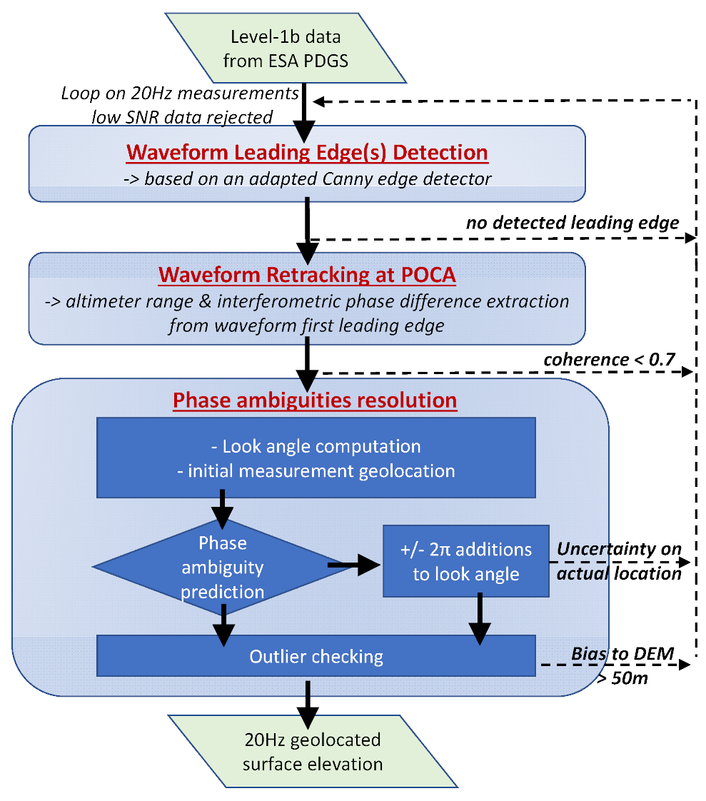
In this section, we present the methodology developed to derive the ice sheet topography from the CryoSat-2 SARInM level-1b data. The processor generates one topography estimate per 20 Hz waveform, geolocated at the estimated across-track POCA. Hence, the measurements are posted at ~300 m intervals along the satellite track. Figure 1 displays the conceptual processing flow chart. It includes three main operating steps: waveform leading edge(s) detection, waveform retracking, and interferometric phase ambiguity resolution. Prior to these operations, the Signal to Noise Ratio (SNR) is checked by means of the backscattering coefficient (Sigma-0) provided in the PDGS level-2 products. If the Sigma-0 is lower than −10 dB we consider the waveform too noisy, as it was found that below −10 dB, the ratio of processing failures begins to exponentially increase. Over the Antarctic ice sheet, approximately 4% of the data measured have a Sigma-0 estimated lower than −10 dB.

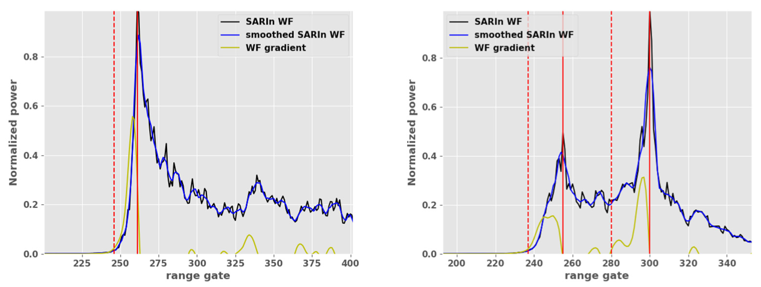
The first processing step objective is to identify the leading edges considered significant in the CryoSat-2 SARInM waveform. In fact, since the ice sheet topography can be irregular and rugged at the footprint scale, the waveform leading edge is not always clearly noticeable, and backscattered energy from different on-ground locations can create different energy peaks on the waveform, potentially mixed together. The energy peaks are identified with the Leading Edge Detection (LED) module, an algorithm developed and inspired from the Canny edge detector [20], adapted to the CryoSat-2 SARInM waveform. In this study, only the first detected leading edge was used in the aftermath to derive surface elevation at POCA, an approach also followed by other groups [21,22,23]. An illustration of the algorithm application on two SARInM waveforms measured over Antarctica is presented in Figure 2.

The second processing step is the so-called waveform retracking. In the processing developed, its purpose is to derive the epoch parameter (or retracking point) from the waveform. To this end, the sample with the highest coherence in the waveform leading edge top-half portion is selected. We refer to this new approach as the Leading Edge maximum Coherence (LMC) retracker. More details related to this retracking algorithm are presented Section 3.5 and Section 4. Compared to state-of-the-art, we consider that the main innovations are in these first two processing stages: waveform leading edge detection and waveform retracking.

During the third and last processing step, surface elevation is estimated from the radar round-trip delay derived at the retracking point. The topography estimation is corrected for additional delays due to ionosphere and troposphere, and for effects due to solid Earth tide, pole tide, and ocean loading tide. These geophysical corrections are available in the PDGS level-1b products. Following the established SARIn principles, the measurement location is computed using the interferometric phase difference at the retracking point [21]. Since mispointing angles’ accuracy is improved in the PDGS Baseline-D products, no additional corrections were applied to the estimated look angle, following recommendations from Meloni et al. [24]. By means of an auxiliary DEM, potential interferometric phase ambiguities are detected and resolved by adding or subtracting 2π to the phase difference value [21,22,23]. The elevation solution the closest to the DEM is finally kept, except if solutions close to each other are detected, separated by less than 15 m in the absolute elevation bias to the DEM. This is theoretically possible, as the POCA can geometrically correspond to different on-ground locations within the measurement footprint. In these situations, we thus consider there is an uncertainty on the measurement geolocation, and the measurement is discarded. Following the approach of other groups [21,22,23], measurements with a coherence value lower than 0.7 at the retracking point are also discarded. Finally, outliers are removed if the estimated elevation deviates more than 50 m to the reference DEM. A more complete technical description of the newly developed SARIn level-2 processing chain is available in Supplementary Materials, Sections S1–S3.

The auxiliary DEMs employed to check interferometric phase ambiguities and elevation outliers were the Reference Elevation Model of Antarctica (REMA) [25] and the ArcticDEM from the Polar Geospatial Center [26]. The ArcticDEM and REMA were respectively used at 100 m and 200 m spatial resolution. CryoSat-2 measurements were spatially selected over the polar ice sheets, using the surface flag from the BedMachine dataset (v1 over Antarctica; v3 over Greenland) [27].

CryoSat-2 SARInM level-1b, level-2, and level-2i products generated by the ESA PDGS ICE Baseline-D were used for this study. Compared to the previous Baseline-C, the Baseline-D data quality over ice sheet is enhanced thanks to a better estimation of the mispointing angles (roll, pitch, and yaw) and a new CAL4 calibration correction, theoretically improving the SARInM interferometric phase difference and coherence at the retracking point. The upgrades brought to the CryoSat-2 ICE Baseline-D products are described in detail in Meloni et al. [24]. Level-1b products are the input data of the CLS level-2 processing chain. Surface elevations available in the level-2 products were extracted to be compared with the CLS processing estimations. Different quality and data flags from level-2 and level-2i products were also used in the analyses; they are listed in Supplementary Materials, Section S5. In addition, to fairly compare the performances of the CLS and PDGS processing chains, the PDGS elevation outliers were also detected and removed if the estimated elevation deviated more than 50 m to the reference DEM, the same threshold as used in the CLS processor.

2.3. Evaluation over Austfonna Ice Cap, Svalbard

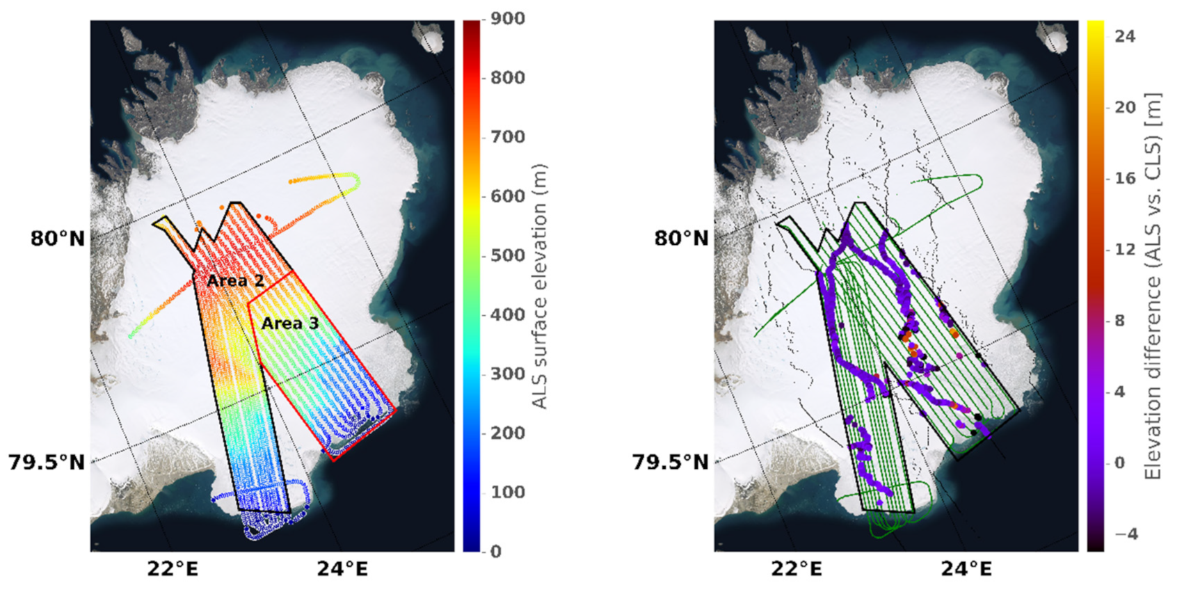
Austfonna is an ice cap located in Norway’s Svalbard archipelago. Covering an area of 7800 km², it is Europe’s third-largest glacier by area and volume and is included in the CryoSat-2 SARInM geographical mask. In 2016, in the frame of a CryoVEx airborne campaign, parts of the Austfonna ice cap were measured by near-infrared Airborne Laser Scanner (ALS) to assess the CryoSat-2 SARInM performances over the region. To maximize the numbers of co-located measurements between ALS and CryoSat-2 SARInM data, the airborne flights sampled the ice cap surface in parallel lines with a spacing of 1 or 2 km next to the CryoSat-2 nadir ground tracks.

As displayed in Figure 3, the whole sampled area (“area 1”) is split into two regions, the west part where the topography is relatively smooth for a large area portion (“area 2”) and the southeast part where the topography is more complex and challenging for radar altimeters (“area 3”). Sandberg Sørensen et al. (2018) [12] used the ALS dataset to evaluate SARInM elevations derived from several processing chains:

⮚

The AWI land ice processing, with and without the use of a DEM [22];

⮚

The NASA Jet Propulsion Laboratory land ice CryoSat processing [23];

⮚

The Technical University of Denmark (DTU) Advanced Retracking System (LARS NPP50 [28]);

⮚

The University of Ottawa (UoO) CryoSat processing [21,29].

For each CryoSat-2 elevation, the corresponding ALS elevation is computed at the radar location using linear interpolation in the airborne data grid. Detailed information about the benchmark can be found in Sandberg Sørensen et al. [12]. We reproduced the benchmark diagnoses using the shared code provided as supplementary material to their publication. The elevations available in the PDGS Baseline-D level-2 products and those generated by the CLS level-2 processing were added to the assessments. To enable a comparison as fair as possible with most of the other benchmarked processing chains, we selected PDGS Baseline-D elevations with a coherence value higher than 0.7 at the retracking point. In addition, the elevation outliers were identified and removed from the statistics if the absolute elevation bias between the SARInM estimation and the interpolated Arctic DEM was larger than 50 m. This editing was applied to all the processing chains evaluated for the sake of fairness. This most likely explains the differences observed in the retrieved statistics compared to Sandberg Sørensen et al. [12] and Meloni et al. [24].

The statistics of the elevation differences between CryoSat-2 and ALS are given in

Table 1. Elevation statistics between SARIn CS2 and ALS, over the Austfonna ice caps, from Sandberg Sørensen et al. [12], updated with the inclusion of the CLS and ESA PDGS ICE Baseline-D estimations.

Area	CS2 Data Set	AWI Baseline-C Inputs)	AWI-DEM (Baseline-C Inputs)	JPL (Baseline-C Inputs)	LARS (Baseline-C Inputs)	UuO (Baseline-C Inputs)	ESA PDGS Baseline-D	CLS (Baseline-D Inputs)
1	# of Δh	817 (510)	783 (510)	718 (510)	729 (510)	752 (510)	657 (510)	720 (510)
	Mean (m)	3.66 (3.4)	4.59 (3.06)	0.19 (0.06)	5.58 (5.81)	0.93 (0.33)	−1.08 (−1.01)	0.2 (0.32)
	Median (m)	2.34 (2.19)	2.04 (1.91)	−0.3 (−0.17)	5.16 (5.39)	−0.31 (−0.53)	−1.17 (−1.15)	−0.17 (−0.16)
	STD (m)	5.86 (4.26)	11.73 (4.14)	4.49 (3.45)	8.97 (6.62)	4.8 (4.08)	4.44 (3.49)	3.43 (3.11)
2	# of Δh	510 (393)	506 (393)	469 (393)	490 (393)	497 (393)	454 (393)	476 (393)
	Mean (m)	2.39 (2.28)	4.22 (1.97)	−0.48 (−0.28)	5.53 (5.95)	−0.56 (−0.62)	−1.41 (−1.24)	−0.18 (−0.11)
	Median (m)	2.02 (1.98)	1.61 (1.53)	−0.34 (−0.27)	5.53 (5.65)	−0.87 (−0.9)	−1.17 (−1.16)	−0.27 (−0.21)
	STD (m)	3.97 (1.89)	12.41 (1.91)	2.93 (1.77)	7.28 (5.72)	1.97 (1.83)	3.12 (2.19)	1.78 (1.44)
3	# of Δh	309 (111)	278 (111)	252 (111)	239 (111)	256 (111)	203 (111)	244 (111)
	Mean (m)	5.73 (7.3)	5.27 (6.84)	1.35 (1.24)	5.67 (5.21)	3.84 (3.46)	−0.34 (−0.21)	0.93 (1.83)
	Median (m)	3.97 (5.26)	3.78 (4.44)	−0.14 (0.22)	4.72 (4.86)	1.59 (0.99)	−1.09 (−1.09)	0.11 (0.41)
	STD (m)	7.61 (6.87)	10.33 (6.58)	6.33 (6.44)	11.7 (8.93)	6.88 (6.78)	6.43 (6.15)	5.26 (5.78)

. Since the benchmarked level-2 processing have their own procedures to detect the waveform leading edge, perform the retracking, geolocate the data, reject noisy waveforms… the number of elevations produced at 20 Hz rate was not the same between the data set examined. Moreover, the population of elevation outliers discarded was also not equivalent between the processors. The amount of CryoSat-2 SARInM 20 Hz measurements assessed varied from 657 (PDGS) to 817 (AWI). The numbers in brackets in Table 1 correspond to a common selection, where the same 20 Hz acquisitions were compared.

By considering the whole area and the measurements included in the common selection, we noticed that the standard deviation of the heights difference was approximately between 3 m and 4 m for most of the processing chains evaluated: 3.11 m (CLS), 3.45 m (JPL), 3.49 m (PDGS), 4.08 m (UuO), and 4.14 m (AWI-DEM). In terms of accuracy, CLS and JPL processors provided the lowest biases to ALS elevations: median biases were −21 cm and −27 cm over area 2; +41 cm and +22 cm over area 3, respectively, with the CLS and JPL processors.

In the different quality tests performed by the CLS processor, it must be noted that 34 measurements were discarded due to an uncertainty on the surface location. We underline that this benchmark helped us refine the 15 m threshold employed to detect such scenarios. It was found that this conservative threshold is valuable to remove large elevation outliers, with the counterpart of a less amount of 20 Hz elevations generated. Nevertheless, it will be shown in Section 3 that only ~2% of measurements were discarded over Antarctica due to this criterion alone.

CLS processor also benefits from the improvements made on the Baseline-D level-1b data, while the other processors’ estimations are derived from Baseline-C level-1b data. An update of this benchmark will thus enable fairer comparisons. Finally, it is also worth noticing that area 3 is characterized by a rough topography with many deep crevasses, as reported in Sandberg Sørensen et al. [12]. Therefore, a linear interpolation made on the ALS 2 km elevation grid might not be sufficient to fairly reproduce the exact topography, potentially explaining the lower agreement between CryoSat-2 and ALS over this area.

3. CryoSat-2 and ICESat-2 Comparison over Antarctica

3.1. CryoSat-2 SARInM Data Set

CryoSat-2 SARInM ice sheet elevations from the PDGS level-2 products and the CLS level-2 processing were analyzed in this study. Measurements were selected over a period from 1 May 2019 to 5 May 2020, covering the 369 days duration of the CryoSat-2 orbit cycle. This long cycle has the advantage of short inter-track distances compared to other altimetry missions. For instance, at 70° S the across-track spacing between adjacent tracks is 2.6 km on average, decreasing at lower latitudes down to 88° S, where the nadir tracks converge.

Approximately 19 million 20 Hz level-1b/level-2 SARInM acquisitions were selected over the Antarctic CryoSat-2 SARInM mask, and the period considered. No changes were applied to the processing chain configuration with respect to the version used for the Austfonna evaluation, presented in Section 2.3. After quality selection, surface topography was successfully retrieved for 88.65% and 71.46% of the measurements, respectively, for the CLS and the PDGS level-2 processing. Table S1 in Supplementary Materials provides the ratio of discarded measurements at each processing step and quality control. The lowest significant amount of data finally retained from the PDGS data set is explained by the selection made on the coherence value, and the choice to discard measurements in case of interferometric phase ambiguity warning. Both criteria lower the amount of data kept by ~25%. But without this restrictive selection, the performances obtained are significantly degraded.

3.2. ICESat-2 ATL06 Data Set

The NASA ICESat-2 mission launched in September 2018 carries a single instrument onboard: the Advanced Topographic Laser Altimeter System (ATLAS), a photon-counting laser altimeter using 532 nm wavelength laser pulses [10]. The six individual ATLAS beams are arranged in three pairs, each pair being constituted by a weak and a strong beam separated by 90 m in across-track to provide a local slope estimation. The three pairs of beams are separated by 3 km across track. In this study, only the ICESat-2 measurements acquired by the strong beams were selected to lighten the considerable amount of data analyzed. The spatial footprint of each ICESat-2 laser pulse is about 17 m in diameter. ICESat-2 orbit completes a cycle after 91 days, the maximal across-track spacing between two beam tracks reaches ~4 km at 70° S. The orbit inclination is the same as CryoSat-2, providing coverage of Antarctica down to 88° S.

ICESat-2 data are available at different format levels, from the reformatted telemetry to surface-specific gridded products generated by thematic experts. In this study, the ATL06 product was used (release 003), providing land ice elevations posted at 40 m along the six ground track beams. The delivered elevations were corrected from different geophysical effects, such as tidal and atmospheric ones. Bad quality data were discarded using the binary “atl06_quality_summary” product flag. As with the CryoSat-2 data set, the spatial selection over the Antarctic ice sheet was performed using the surface flag from the BedMachine dataset [27]. Overall, approximately 3240 million ATL06 elevation measurements were selected over the Antarctic ice sheet, acquired from 1 March 2019 to 5 September 2020. This data set included all the acquisitions made over the Antarctic ice sheet, not only those included in the CryoSat-2 SARInM geographical mask. Thanks to the homogeneous and dense coverage provided by the ICESat-2 ATL06 data set, it was possible to find a large population of space–time coincident observations with CryoSat-2, worthwhile to build robust statistics at a continental scale, as presented in the following sections. Considering that only the ICESat-2 strong beams measurements were integrated into the analyses, these statistics can be potentially expanded.

3.3. Point-to-Point Methodology

Mono-mission and multi-mission crossovers are usually employed over ocean to assess the altimeter performances. In this approach, the surface topography is interpolated at the point where the two nadir ground tracks intersect. Over ice sheet, this methodology is complex to set up, mainly due to the topography variations at the along-track sampling scale (~300 m), creating uncertainties in the interpolation process. In this study, we, therefore, employed a “Point-to-Point” method, as already used by Wang et al. [7] for a similar and previous comparison between CryoSat-2 and the original ICESat. In this method, the along-track elevations from both sensors are compared if the measurements are co-located in space and time. Considering the 40 m posting rate of ICESat-2, a search radius of 20 m was used in this study to find co-located measurements. This ensured that a single 20 Hz CryoSat-2 measurement would not be co-located with two consecutive ICESat-2 ATL06 measurements, and therefore not duplicated in the statistics. As a trade-off between robust statistics and accuracy, the maximal time span between the acquisitions was set to 60 days.

Inherent errors to the Point-to-Point method are associated with the space and time differences between the two sensor measurements. Over a terrain slope of 0.5°, as encountered on average over the Antarctica CryoSat-2 SARInM mask, the theoretical elevation error is ~9 cm in the worst case, when measurements are distant of 20 m. For a large part of Antarctica, where the ice topography variation remains below +/−50 cm/yr [30], the maximal theoretical elevation error induced by surface elevation change between sensors acquisitions is below 10 cm. Finally, as the across-track spacing is reduced close to the poles, the number of co-located measurements significantly increases at the lowest latitudes covered. To avoid a statistical oversampling of these areas, the acquisitions made at latitudes lower than 80° S were not selected.

Over the whole year analyzed, 249,823 and 209,960 CryoSat-2 and ICESat-2 co-located elevations were identified, respectively, with the CLS and PDGS SARInM data set. For each co-located point, the elevation difference was computed as CryoSat-2 minus ICESat-2. No further filtering was applied to the data, and elevation difference outliers remained present in the statistics presented next section.

3.4. Results

In order to quantify the bias and the dispersion between CryoSat-2 and ICESat-2 elevations, we respectively computed the Median bias and Median Absolute Deviation (MAD) of the co-located elevation differences. The MAD being defined as:

MAD = median (|Δh − median(Δh)|)

(1)

where Δh are the CryoSat-2 and ICESat-2 co-located elevation differences. Both median bias and MAD allow mitigating the impact of large outliers in the statistics. Moreover, in order to estimate and analyze the outliers population, we arbitrarily considered a “large outlier” as an absolute elevation difference greater than 5 m. Statistics obtained with other threshold values are presented in Supplementary Materials. The median bias, MAD, and outliers’ ratio of the CryoSat-2 and ICESat-2 elevation differences are shown in Figure 4, represented as a function of the nadir surface slope derived from REMA. The surface slope was computed at a 15 km scale around nadir. In Figure 5, the median bias and MAD are mapped using an 80 km stereographic grid with a standard parallel of 71° S. The grid resolution was chosen to maximize the continent coverage, with at least 100 co-located elevations per box.

Overall, the agreement between CryoSat-2 and ICESat-2 is found better in accuracy and precision with SARInM estimations derived from the CLS processing. The median elevation bias with ICESat-2 is −17.8 cm, and this bias is weakly affected by the surface slope, remaining between −15 cm and −20 cm when the slope magnitude is between 0° and 1.5°. Nonetheless, geographical patterns showing more important spatial variations are noticeable on the map in Figure 5. The exact origins of these regional patterns are not yet explained and would require dedicated regional analyses, out of scope for this study. The impacts of snow volume scattering and surface roughness have to be investigated, as discussed in Section 4. In the map in Figure 5, the median elevation bias obtained with the CLS processing is between −40 cm and 0 cm for ~92% of the 80 km boxes displayed.

With the CLS processing, the MAD of the elevation differences is on average 46.5 cm. This value linearly increases as a function of surface slope, from about 30 cm for surface slopes below 0.2° to ~1.1 m on average for surface slopes higher than 1°. These statistics integrate the uncertainties of the two measures, along with the inherent temporal and spatial errors due to the Point-to-Point method. Reducing the spatial–temporal selection of co-located measurements, from 20 m to 5 m in distance and 60 days to 10 days in time, does not significantly reduce the dispersion between CryoSat-2 and ICESat-2 elevations, as the MAD of the elevation differences is lowered from 46.5 cm to 43.3 cm only. With the PDGS processing, the MAD of the elevation differences is 80.4 cm on average. The measurement precision achieved by the CLS processing is thus significantly improved, by about 42%. This difference is further analyzed and discussed Section 4. As expected, the number of large outliers increases with the surface slope magnitude. With the CLS processing, ~6% of the elevation differences are larger than 5 m when the surface slope is about 1.5°. This ratio decreases to 0.36% for measurements acquired over surface slopes lower than 0.5°.

In the diagnoses displayed in Figure 4, the statistics are represented as a function of the surface slope. Figure S2 available in Supplementary Materials represents the same statistics as a function of the on-ground distance between satellite nadir and the estimated SARInM measurement geolocation. The analysis shows that SARInM measurement locations can be distant up to 10 km from nadir, in the across-track direction. This corresponds to an across-track surface slope of ~0.9° in the case of a linear surface. Scatterers sampled at such off-nadir distance are outside of the area illuminated by the antenna aperture at −3 dB, which extends to ~7 km around nadir. The results demonstrate that for those measurements, the altimeter is still capable of measuring reliable topography elevations, nonetheless with a degraded precision.

3.5. Assessment of the Leading Edge Maximum Coherence Retracking Algorithm

Among the new algorithms developed in the CLS level-2 processing chain, the chosen retracking method deserves additional considerations in light of its key role in the processing. Currently, two main retracking approaches are employed by scientific groups working with SARInM data over ice sheet. A first method proposed by Davis et al. [31] and adapted by Helm et al. [22] with the Threshold First Maximum Retracking Algorithm (TFMRA), consists in estimating the retracking point on the first waveform leading edge, at a pre-defined threshold related to the leading edge maximum normalized power. A second approach consists in estimating the retracking point by searching the Leading Edge maximum Gradient (LMG retracker), as proposed initially by Gray et al. [21] and re-adapted by Nilsson et al. [23]. In addition to these methods, the PDGS processor employs a theoretical semi-analytical model to fit the SARInM waveform.

In the new algorithm developed for this study, and as described in Section 2.2, the retracking point is positioned at the sample with the highest coherence in the waveform leading edge top-half portion. The retracker focuses on this specific part of the leading edge (i.e., between 50% and 100% of waveform peak maximum power) as it was demonstrated that the first surface return is located close to the leading edge maximum power [6]. In the CLS processing chain, the LMC retracker was substituted with a threshold retracker and a maximum gradient retracker. The implementation details of these algorithms are available Section S4 in Supplementary Materials. The three retrackers focus on the same waveform leading edge, identified preliminarily by the Leading Edge Detection (LED) module of the CLS processing chain.

For the threshold retracker, a 50% threshold value was chosen as it provided the best performances in terms of accuracy and precision compared to the 25% and 75% threshold values. In terms of accuracy, by considering ICESat-2 as the true elevation at snow/air interface, it must be noted that the surface elevation was on average overestimated if the retracking threshold is below ~50%, and on average underestimated if the retracking threshold is above ~50% (see Figure S3 in Supplementary Materials). These conclusions apply to measurements acquired over relatively flat surfaces (slope below 0.25%). When the surface slope increases, on average, the needed threshold to derive surface elevation at the snow/air interface increases. Similar results were reported by Nilsson et al. [23]; in their study, a 40% threshold was necessary to avoid positive or negative biases between CryoSat-2 SARInM and Icebridge Airborne Topographic Mapper (ATM) elevations over the studied areas in Greenland.

In Figure 6, the statistics presented in Section 3.4 (Figure 4) are reproduced with the 50% threshold retracker (green) and the gradient retracker (orange). On average, the MAD between CryoSat-2 and ICESat-2 elevations are 41.2 cm, 46.5 cm, and 48.8 cm, respectively, obtained with the threshold, LMC, and gradient retrackers. The threshold retracker provides the best precision over the low-moderate slopes, below 0.8°, while the LMC retracker is better over higher topographic slopes. On average, the median differences between CryoSat-2 and ICESat-2 elevations are −17.8 cm, 10.9 cm, and 11.6 cm, respectively, obtained with the LMC, gradient, and threshold retrackers. The elevation difference derived from the gradient and the threshold retrackers is found to be sensitive to the topographic surface slope. With these two algorithms, the median elevation bias is ~5 cm over the lowest surface slopes, below 0.1°. This difference increases to 30 cm and 50 cm over surface slopes ~1.5°, respectively, with the gradient and the threshold retrackers. In contrast, as previously stated, the elevation accuracy obtained with the LMC retracker appears to be less affected by the surface slope. This outcome can also be observed in Figures S4 and S5 in Supplementary Materials, showing the spatial variations of the elevation differences between CryoSat-2 and ICESat-2 over Antarctica, for the three retracking methods analyzed.

4. Discussion

As stated in Section 2.1, the altimetry waveforms acquired over ice sheets are impacted by different properties of the surface sampled. In particular, it is well established that the surface topography variation within the measurement footprint can strongly affect the waveform leading edge and the waveform shape in general. While the waveforms measured over linear surfaces with moderate slopes below 1° exhibit a relatively clear unique leading edge, the waveforms acquired over steeper or rugged topographies have more diverse and complex shapes. Therefore, it is also instructive to assess the performances achieved as a function of the waveform shape parameters. This indicates the processing capabilities to adjust to different types of acquisitions. For that purpose, the developed LED algorithm provides helpful information relative to the leading edge shape, such as the width, energy, gradient.

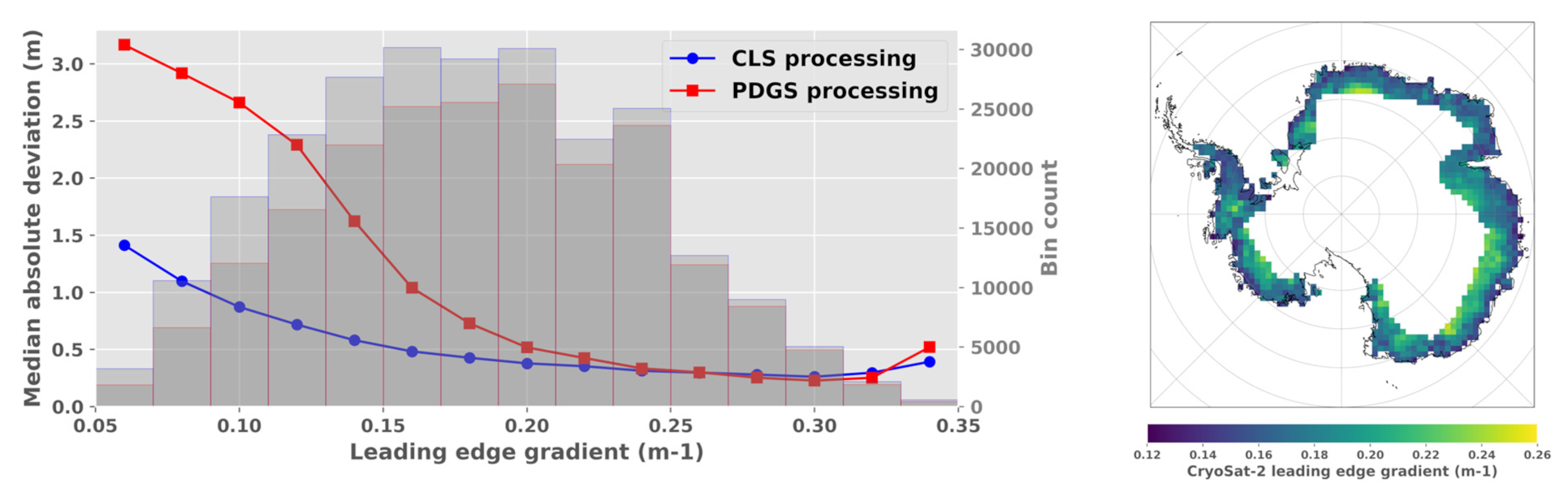
In Figure 7, we chose to represent the MAD between CryoSat-2 and ICESat-2 elevations as a function of the CryoSat-2 waveform leading edge gradient. Based on theoretical studies [6], we assumed that the waveform leading edge gradient is maximum over a flat surface, and decreases with the influence of the surface slope and roughness. The results show that the CLS and PDGS processors achieve a similar precision for the steepest waveform leading edges (above 0.25 m⁻¹). Non-surprisingly, the map Figure 7 evidences that these measurements were acquired over the inland part of the SARInM mask, where the surface topography is flatter and more linear compared to coastal areas. However, closer to the coast, where the waveform leading edge gradient on average decreases, the precision obtained with the PDGS processing is clearly degraded compared to the CLS one.

The differences observed between the CLS and PDGS processors are likely partly explained by the different retracking strategies followed. In the processing chain developed, the retracking point is estimated in the top-half portion of the first detected leading edge, where the interferometric coherence is maximal. By tracking the highest coherent point, the procedure theoretically maximizes the probability to select a radar return originating from a clear on-ground location. One corollary is that the method necessarily adjusts to any types of waveform leading edges. For its part, the PDGS processor uses a theoretical model to fit the waveforms, an approach complex to set up as the model must be versatile enough to adapt to the different waveform shapes measured over ice sheets.

In this study, the performances were assessed uniquely as a function of the averaged surface slope, derived at the footprint scale. Additional analyses focusing on the surface roughness at different scales (centimeter to kilometer) would also be very instructive. For that purpose, the exploitation of recent high-resolution DEMs generated with stereo imagery [25,26,32] could be valuable to better model the SARInM level-1 signals (waveforms, phase difference, and coherence) in response to realistic surface roughness variations. This would help to further understand the differences obtained between different retracking methods. This could also be beneficial for the development of new retracking concepts, better accounting for the surface roughness influence on the SARInM measurements.

Another source of uncertainty is related to the complex interaction between the Ku band radar wave signal with the snow medium. As the emitted radar wave penetrates into the snowpack, a subsurface volume scattering signal is backscattered to the satellite. This signal sums-up with the one coming from surface at snow/air interface. This effect is well known in conventional altimetry, disrupting the shape of the LRM waveforms measured, and therefore complicating the topography estimation at the exact snow/air interface [33]. Space and time variations of the snowpack parameters can produce artificial topography variations if they are not accounted for by the retracker, or post-corrected [34,35]. In the Ku band unfocused SAR mode, preliminary analyses made over lake Vostok, Antarctica, showed that the leading edge shape remains relatively as sharp as observed with oceanic acquisitions. Hence, the topography estimated at POCA would be less sensitive to the snow volume scattering effect compared to LRM [14]. Nonetheless, more exhaustive analyses are required at a global scale to quantify the potential topography bias induced by snow volume scattering in SAR/SARIn altimetry, and its temporal and spatial variations, depending on the chosen retracking approach.

As described Section 2, the SARInM level-2 processing includes multiple operations, each of them affecting the surface elevation estimated. For instance: the smoothing of the SARInM level-1 signals, the waveform leading edge detection, the waveform retracking, the phase ambiguities correction, the outlier’s rejection, the thresholds applied to the coherence and SNR values to consider the measurement valid, and any supplementary computations. For each of these operations, different methods have been established by the scientific groups working with SARInM data over land ice [12]. In Section 3.5, three retracking strategies are compared, without any other changes in the level-2 processing chain (for example, the waveform smoothing remains the same for the three retrackers tested). It would be therefore worthwhile to assess the importance of each of the previously mentioned operations in the performances obtained, but this was out of scope of this study.

Finally, it must be noted that the CryoSat-2 SARInM waveforms are subject to a relatively high speckle noise level compared to CryoSat-2 LRM and SAR acquisitions, as the altimeter emits one single burst per 20 Hz radar cycle in SARInM. Comparatively, the onboard altimeter of the future Copernicus Polar Ice and Snow Topography Altimeter (CRISTAL) is planned to have a 4-times higher burst frequency rate, which will reduce substantially the speckle noise level. Furthermore, the CRISTAL altimeter technical characteristics will be improved, in particular, with the use of dual-frequency Ku/Ka bands, and a reduced range vertical resolution, from ~47 cm for CryoSat-2 to ~31 cm for CRISTAL. Thanks to these features, a significant performance improvement is expected with CRISTAL [36].

5. Conclusions

A new level-2 processing chain was developed dedicated to the CryoSat-2 SARInM measurements acquired over ice sheet. The processor includes new revised methods, in particular, to detect waveform leading edges and perform the retracking. One year of CryoSat-2 level-1b acquisitions measured over the Antarctica SARInM geographical mask were processed with this level-2 algorithm. This represents 19 million measurements. The ice sheet topography was successfully retrieved for ~89% of these data.

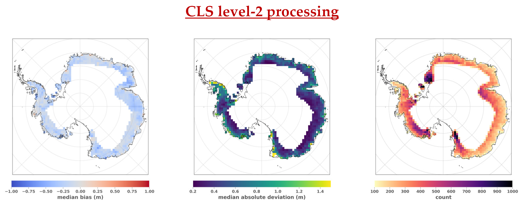
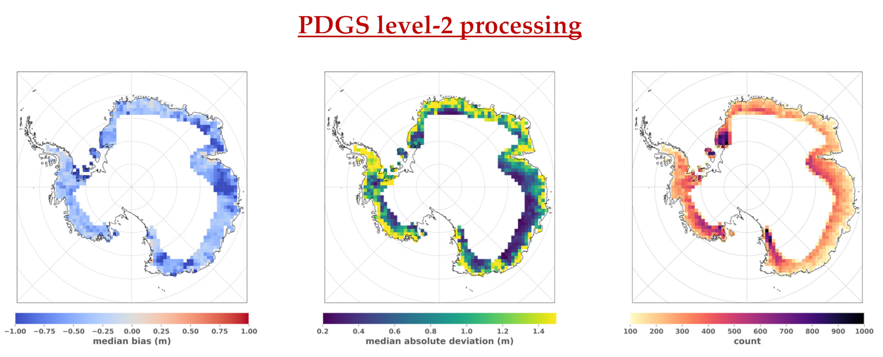
From this data set, about 250,000 space–time nearly coincident observations with ICESat-2 ATL06 measurements were found and examined. Comparison to ICESat-2 quantifies and demonstrates the added value of the newly developed level-2 processing chain. The median elevation bias between CryoSat-2 and ICESat-2 is −17.8 cm, while a bias of −47.3 cm is obtained with CryoSat-2 SARInM elevations from the PDGS level-2 products. The median absolute deviation between CryoSat-2 and ICESat-2 co-located elevations is 46.5 cm, compared to 80.4 cm obtained with the PDGS data. The measurement precision is thus improved by about 42%. This enhancement is particularly observed over areas close to the coast, where the waveform leading edges are less peaky compared to the acquisitions made over the continent’s interior.

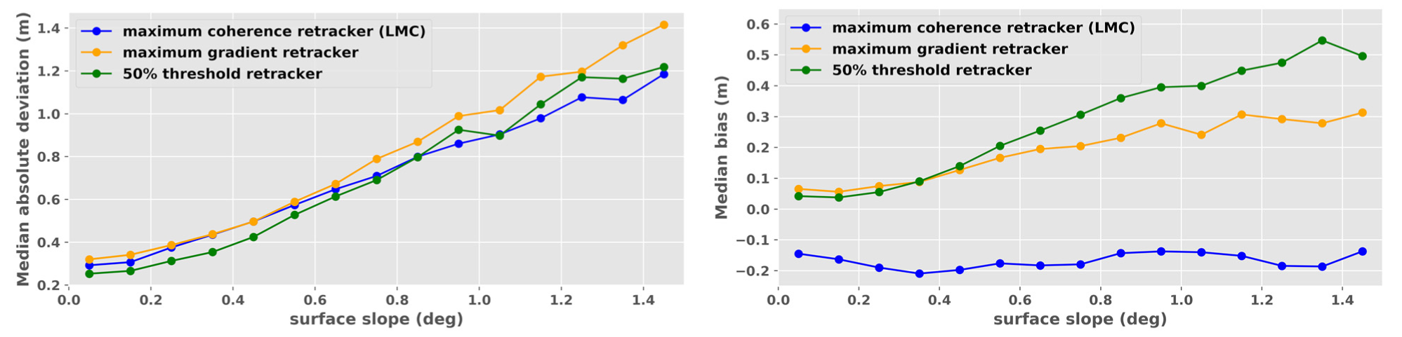
The new Leading edge Maximum Coherence (LMC) retracker developed and implemented in the CLS processing chain was compared to a 50% threshold retracker and a gradient retracker. Results show that the threshold retracker is on average the most performant over surface slopes below 0.8°, but the LMC retracker performs better over higher surface slopes. Moreover, the accuracy obtained with the LMC retracker appears to be less affected by the surface slope compared to the two other retracking algorithms. Nevertheless, the median elevation bias between CryoSat-2 and ICESat-2 still exhibits spatial variations over the continent. Compared to PDGS, these variations are significantly reduced with the CLS processing chain, from one meter to several decimeters’ amplitude. Future dedicated regional analyses will be necessary to assess and understand the origins of these variations. For that purpose, a better understanding and modeling of the SARInM waveforms in response to surface roughness variations (centimeter to kilometer scales) and volume scattering would be insightful.

At the time of its launch, scheduled in 2027, the CRISTAL mission will be most likely the single altimetry mission surveying the cryosphere at high latitudes, between ±81.5° and ±88°. In contrast to CryoSat-2, the altimeter is planned to operate exclusively in SARInM over the polar ice sheets. Evaluations and further improvements of the SARInM performances are therefore of major importance for the mission preparation and future ice sheet mass balance estimates.

References

1. Church, J.A.; Clark, P.U.; Cazenave, A.; Gregory, J.M.; Jevrejeva, S.; Levermann, A.; Merrifield, M.A.; Milne, G.A.; Nerem, R.S.; Nunn, P.D.; et al. The Physical Science Basis. Contribution of Working Group I to the Fifth Assessment Report of the Intergovernmental Panel on Climate Change; Cambridge Univ. Press: Cambridge, UK, 2013; Chapter 13; pp. 1137–1216. [Google Scholar]
2. Shepherd, A.; Ivins, E.; Rignot, E.; Smith, B.; van den Broeke, M.; Velicogna, I.; Whitehouse, P.; Briggs, K.; Joughin, I.; Krinner, G.; et al. Mass balance of the Greenland Ice Sheet from 1992 to 2018. Nature 2020, 579, 233–239. [Google Scholar] [CrossRef]
3. Shepherd, A.; Ivins, E.; Rignot, E.; Smith, B.; van den Broeke, M.; Velicogna, I.; Whitehouse, P.; Briggs, K.; Joughin, I.; Krinner, G.; et al. Mass balance of the Antarctic Ice Sheet from 1992 to 2017. Nature 2018, 558, 219–222. [Google Scholar] [CrossRef] [Green Version]
4. Wingham, D.J.; Francis, C.R.; Baker, S.; Bouzinac, C.; Brockley, D.; Cullen, R.; de Chateau-Thierry, P.; Laxon, S.W.; Mallow, U.; Mavrocordatos, C.; et al. CryoSat: A mission to determine the fluctuations in Earth’s land and marine ice fields. Adv. Space Res. 2006, 37, 841–871. [Google Scholar] [CrossRef]
5. Raney, R.K. The delay/Doppler radar altimeter. IEEE Trans. Geosci. Remote Sens. 1998, 36, 1578–1588. [Google Scholar] [CrossRef]
6. Wingham, D.J.; Phalippou, L.; Mavrocordatos, C.; Wallis, D. The mean echo and echo cross product from a beamforming interferometric altimeter and their application to elevation measurement. IEEE Trans. Geosci. Remote Sens. 2004, 42, 2305–2323. [Google Scholar] [CrossRef]
7. Wang, F.; Bamber, J.L.; Cheng, X. Accuracy and Performance of CryoSat-2 SARIn Mode Data Over Antarctica. IEEE Geosci. Remote Sens. Lett. 2015, 12, 1516–1520. [Google Scholar] [CrossRef]
8. McMillan, M.; Shepherd, A.; Muir, A.; Gaudelli, J.; Hogg, A.E.; Cullen, R. Assessment of CryoSat-2 interferometric and non-interferometric SAR altimetry over ice sheets. Adv. Space Res. 2018, 62, 1281–1291. [Google Scholar] [CrossRef]
9. Zwally, H.J.; Schutz, B.; Abdalati, W.; Abshire, J.; Bentley, C.; Brenner, A.; Bufton, J.; Dezio, J.; Hancock, D.; Harding, D.; et al. ICESat’s laser measurements of polar ice, atmosphere, ocean, and land. J. Geodyn. 2002, 34, 405–445. [Google Scholar] [CrossRef] [Green Version]
10. Markus, T.; Neumann, T.; Martino, A.; Abdalati, W.; Brunt, K.; Csatho, B.; Farrell, S.; Fricker, H.; Gardner, A.; Harding, D.; et al. The Ice, Cloud, and land Elevation Satellite-2 (ICESat-2): Science requirements, concept, and implementation. Remote Sens. Environ. 2017, 190, 260–273. [Google Scholar] [CrossRef]
11. Brunt, K.M.; Smith, B.E.; Sutterley, T.C.; Kurtz, N.T.; Neumann, T.A. Comparisons of Satellite and Airborne Altimetry With Ground-Based Data From the Interior of the Antarctic Ice Sheet. Geophys. Res. Lett. 2021, 48, e2020GL090572. [Google Scholar] [CrossRef]
12. Sandberg Sørensen, L.; Simonsen, S.B.; Langley, K.; Gray, L.; Helm, V.; Nilsson, J.; Stenseng, L.; Skourup, H.; Forsberg, R.; Davidson, M.W.J. Validation of CryoSat-2 SARIn Data over Austfonna Ice Cap Using Airborne Laser Scanner Measurements. Remote Sens. 2018, 10, 1354. [Google Scholar] [CrossRef] [Green Version]
13. Brenner, A.C.; Blndschadler, R.A.; Thomas, R.H.; Zwally, H.J. Slope-induced errors in radar altimetry over continental ice sheets. J. Geophys. Res. Ocean. 1983, 88, 1617–1623. [Google Scholar] [CrossRef]
14. Aublanc, J.; Moreau, T.; Thibaut, P.; Boy, F.; Rémy, F.; Picot, N. Evaluation of SAR altimetry over the antarctic ice sheet from CryoSat-2 acquisitions. Adv. Space Res. 2018, 62, 1307–1323. [Google Scholar] [CrossRef]
15. McMillan, M.; Muir, A.; Shepherd, A.; Escolà, R.; Roca, M.; Aublanc, J.; Thibaut, P.; Restano, M.; Ambrozio, A.; Benveniste, J. Sentinel-3 Delay-Doppler altimetry over Antarctica. Cryosphere 2019, 13, 709–722. [Google Scholar] [CrossRef] [Green Version]
16. Jensen, J.R. Angle measurement with a phase monopulse radar altimeter. IEEE Trans. Antennas Propag. 1999, 47, 715–724. [Google Scholar] [CrossRef]
17. Cullen, R.; Wingham, D.J.; Viau, P.; Francis, C.R.; Mavrocordatos, C. ESA’s CryoSat-2 multi-mode level 0 to level 1B science processors—Algorithm design and pre-launch verification with ASIRAS. In Proceedings of the Envisat Symposium, Montreux, Switzerland, 23–27 April 2007. [Google Scholar]
18. Rémy, F.; Parouty, S. Antarctic Ice Sheet and Radar Altimetry: A Review. Remote Sens. 2009, 1, 1212–1239. [Google Scholar] [CrossRef] [Green Version]
19. Brown, G. The average impulse response of a rough surface and its applications. IEEE Trans. Antennas Propag. 1977, 25, 67–74. [Google Scholar] [CrossRef]
20. Canny, J. A computational approach to edge detection. IEEE Trans. Pattern Anal. Mach. Intell. 1986, 8, 679–698. [Google Scholar] [CrossRef] [PubMed]
21. Gray, L.; Burgess, D.; Copland, L.; Cullen, R.; Galin, N.; Hawley, R.; Helm, V. Interferometric swath processing of Cryosat data for glacial ice topography. Cryosphere 2013, 7, 1857–1867. [Google Scholar] [CrossRef] [Green Version]
22. Helm, V.; Humbert, A.; Miller, H. Elevation and elevation change of Greenland and Antarctica derived from CryoSat-2. Cryosphere 2014, 8, 1539–1559. [Google Scholar] [CrossRef] [Green Version]
23. Nilsson, J.; Gardner, A.; Sandberg Sørensen, L.; Forsberg, R. Improved retrieval of land ice topography from CryoSat-2 data and its impact for volume-change estimation of the Greenland Ice Sheet. Cryosphere 2016, 10, 2953–2969. [Google Scholar] [CrossRef] [Green Version]
24. Meloni, M.; Bouffard, J.; Parrinello, T.; Dawson, G.; Garnier, F.; Helm, V.; Di Bella, A.; Hendricks, S.; Ricker, R.; Webb, E.; et al. CryoSat Ice Baseline-D validation and evolutions. Cryosphere 2020, 14, 1889–1907. [Google Scholar] [CrossRef]
25. Howat, I.M.; Porter, C.; Smith, B.E.; Noh, M.-J.; Morin, P. The Reference Elevation Model of Antarctica. Cryosphere 2019, 13, 665–674. [Google Scholar] [CrossRef] [Green Version]
26. Porter, C.; Morin, P.; Howat, I.; Noh, M.; Bates, B.; Peterman, K.; Keesey, S.; Schlenk, M.; Gardiner, J.; Tomko, K.; et al. ArcticDEM; V1; Harvard Dataverse: Cambridge, MA, USA, 2018. [Google Scholar] [CrossRef]
27. Morlighem, M.; Rignot, E.; Binder, T.; Blankenship, D.; Drews, R.; Eagles, G.; Eisen, O.; Ferraccioli, F.; Forsberg, R.; Fretwell, P.; et al. Deep glacial troughs and stabilizing ridges unveiled beneath the margins of the Antarctic ice sheet. Nat. Geosci. 2020, 13, 132–137. [Google Scholar] [CrossRef]
28. Villadsen, H.; Deng, X.; Andersen, O.B.; Stenseng, L.; Nielsen, K.; Knudsen, P. Improved inland water levels from SAR altimetry using novel empirical and physical retrackers. J. Hydrol. 2016, 537, 234–247. [Google Scholar] [CrossRef] [Green Version]
29. Gray, L.; Burgess, D.; Copland, L.; Dunse, T.; Langley, K.; Moholdt, G. A revised calibration of the interferometric mode of the CryoSat-2 radar altimeter improves ice height and height change measurements in western Greenland. Cryosphere 2017, 11, 1041–1058. [Google Scholar] [CrossRef] [Green Version]
30. Smith, B.; Fricker, H.A.; Gardner, A.S.; Medley, B.; Nilsson, J.; Paolo, F.S.; Holschuh, N.; Adusumilli, S.; Brunt, K.; Csatho, B.; et al. Pervasive ice sheet mass loss reflects competing ocean and atmosphere processes. Science 2020, 368, 1239–1242. [Google Scholar] [CrossRef] [PubMed]
31. Davis, C.H. A robust threshold retracking algorithm for extracting ice-sheet surface elevations from satellite radar altimeters. In Proceedings of the 1996 International Geoscience and Remote Sensing Symposium, Lincoln, NE, USA, 31 May 1996; Volume 3, pp. 1783–1787. [Google Scholar]
32. Rizzoli, P.; Martone, M.; Gonzalez, C.; Wecklich, C.; Borla Tridon, D.; Bräutigam, B.; Bachmann, M.; Schulze, D.; Fritz, T.; Huber, M.; et al. Generation and performance assessment of the global TanDEM-X digital elevation model. ISPRS J. Photogramm. Remote Sens. 2017, 132, 119–139. [Google Scholar] [CrossRef] [Green Version]
33. Ridley, J.K.; Partington, K.C. A model of satellite radar altimeter return from ice sheets. Int. J. Remote Sens. 1988, 9, 601–624. [Google Scholar] [CrossRef]
34. Davis, C.H.; Zwally, H.J. Geographic and seasonal variations in the surface properties of the ice sheets by satellite-radar altimetry. J. Glaciol. 1993, 39, 687–697. [Google Scholar] [CrossRef] [Green Version]
35. Legrésy, B.; Rémy, F. Altimetric observations of surface characteristics of the Antarctic ice sheet. J. Glaciol. 1997, 43, 265–275. [Google Scholar] [CrossRef] [Green Version]
36. Kern, M.; Cullen, R.; Berruti, B.; Bouffard, J.; Casal, T.; Drinkwater, M.R.; Gabriele, A.; Lecuyot, A.; Ludwig, M.; Midthassel, R.; et al. The Copernicus Polar Ice and Snow Topography Altimeter (CRISTAL) high-priority candidate mission. Cryosphere 2020, 14, 2235–2251. [Google Scholar] [CrossRef]
Figure 1. Flow chart showing the methodology developed to retrieve ice sheet elevations from the PDGS L1b SARIn products.
Remotesensing 13 04508 g001
Figure 2. Illustration of the leading edge detection operation for two random SARInM measurements over the Antarctic ice sheet, showing the normalized waveform (black), normalized smoothed waveform (blue), and waveform gradient (yellow) as computed by the LED algorithm. Red dotted and solid lines respectively display the first and last samples of the detected leading edge(s).
Remotesensing 13 04508 g002
Figure 3. (left) The CryoVEx (Cryosat Validation Experiment) airborne laser scanner (ALS) height data collected over Austfonna in April 2016. (right) Differences between the CryoSat-2 SARIn mode elevation derived by the CLS processing chain at level-2 and elevations mapped with ALS. Outside the area of interest, the CS2 data geolocations are marked with small black dots (black polygon).
Remotesensing 13 04508 g003
Figure 4. Median difference (top), median absolute deviation (middle) between SARIn CryoSat-2 and ICESat-2 ATL06 space–time co-located elevations over the Antarctic ice sheet, as a function of the surface slope. The bottom panel displays the percentage of elevation differences greater than 5 m. SARIn mode elevations were derived from the PDGS level-2 product (red) and from the level-2 CLS processor (blue). Elevations were computed as CryoSat-2 − ICESat-2. Gray bars display the number of co-located measurements for each slope interval.
Remotesensing 13 04508 g004
Figure 5. Gridded statistics of the elevation differences between CryoSat-2 SARIn mode and ICESat-2 ATL06 co-located elevations: median difference (left), median absolute deviation (middle), and box count (right). SARIn mode elevations are derived from the level-2 CLS processing (top) and from the PDGS level-2 products (bottom). Elevations are computed as CryoSat-2 − ICESat-2. Grid resolution is 80 km.
Remotesensing 13 04508 g005aRemotesensing 13 04508 g005b
Figure 6. Median difference (left) and median absolute deviation (right) between SARIn CryoSat-2 and ICESat-2 ATL06 space–time co-located elevations over the Antarctic ice sheet, as a function of the surface slope. SARIn mode elevations are derived from the CLS processing chain with different retrackers: LMC (blue), gradient (orange), and 50% threshold (green). The LMC retracker is the default one within the CLS processor. Elevations are computed as CryoSat-2 − ICESat-2.
Remotesensing 13 04508 g006
Figure 7. (left) Median absolute deviation between SARIn CryoSat-2 and ICESat-2 ATL06 space–time co-located elevations over the Antarctic ice sheet, as a function of the gradient of the CryoSat-2 first detected waveform leading edge. SARIn mode elevations were derived from the PDGS level-2 products (red) and the CLS processing (blue). Gray bars display the number of co-located measurements for each gradient interval. (right) Gridded value of the CryoSat-2 first detected waveform leading edge over the Antarctic ice sheet, only for CryoSat-2 measurements co-located with ICESat-2. Grid resolution is 80 km.
Remotesensing 13 04508 g007