
Automatic Interferogram Selection for SBAS-InSAR Based on Deep Convolutional Neural Networks

Abstract
:1. Introduction
2. Materials and Methods
2.1. Differential Interferogram Phase of the SBAS-InSAR Technology
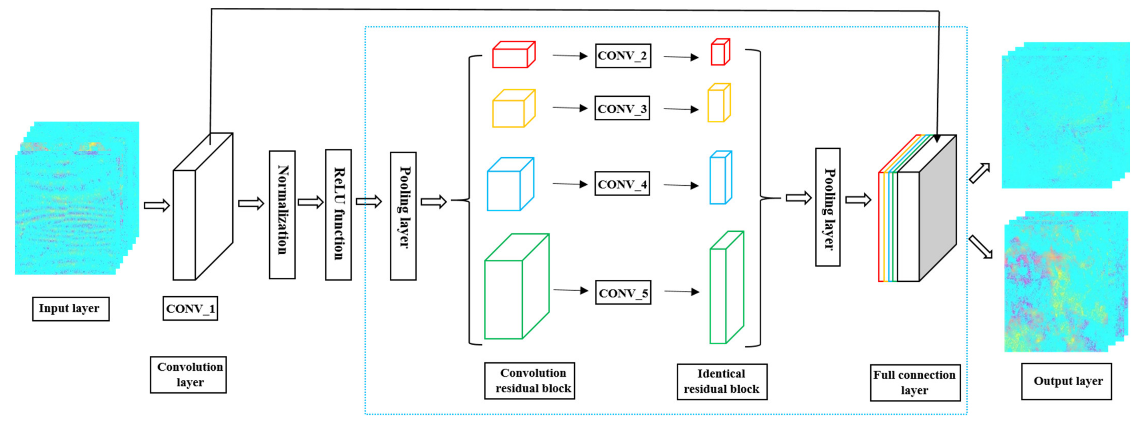
2.2. Deep Convolution Neural Network
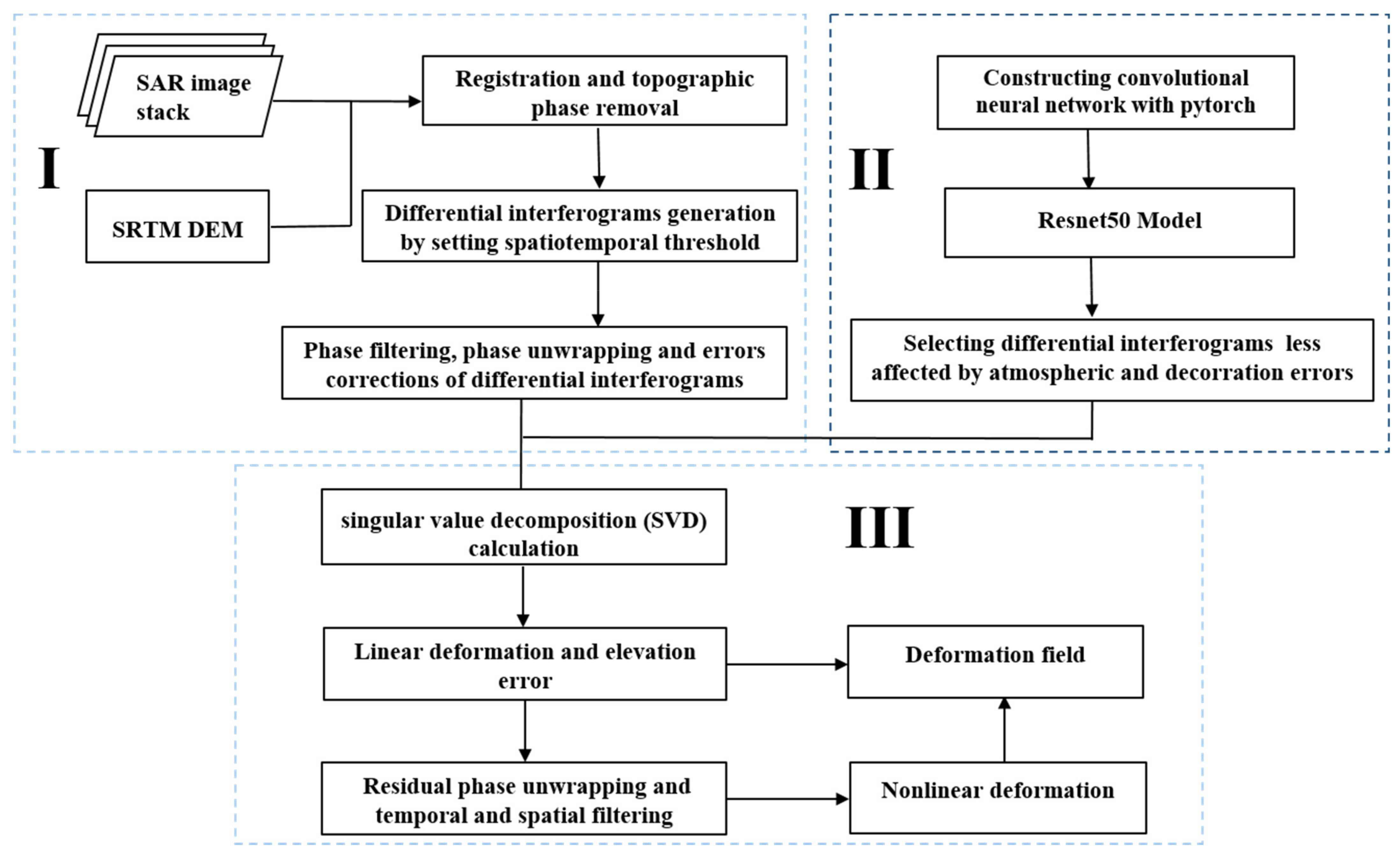
2.3. Automatic Interferogram Selection Using the Proposed Method
2.4. Establishment of Training Sets
3. Results and Discussions
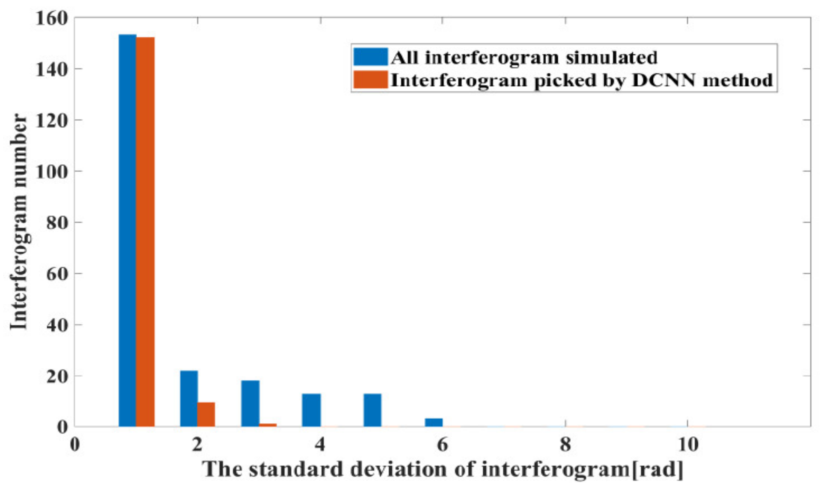
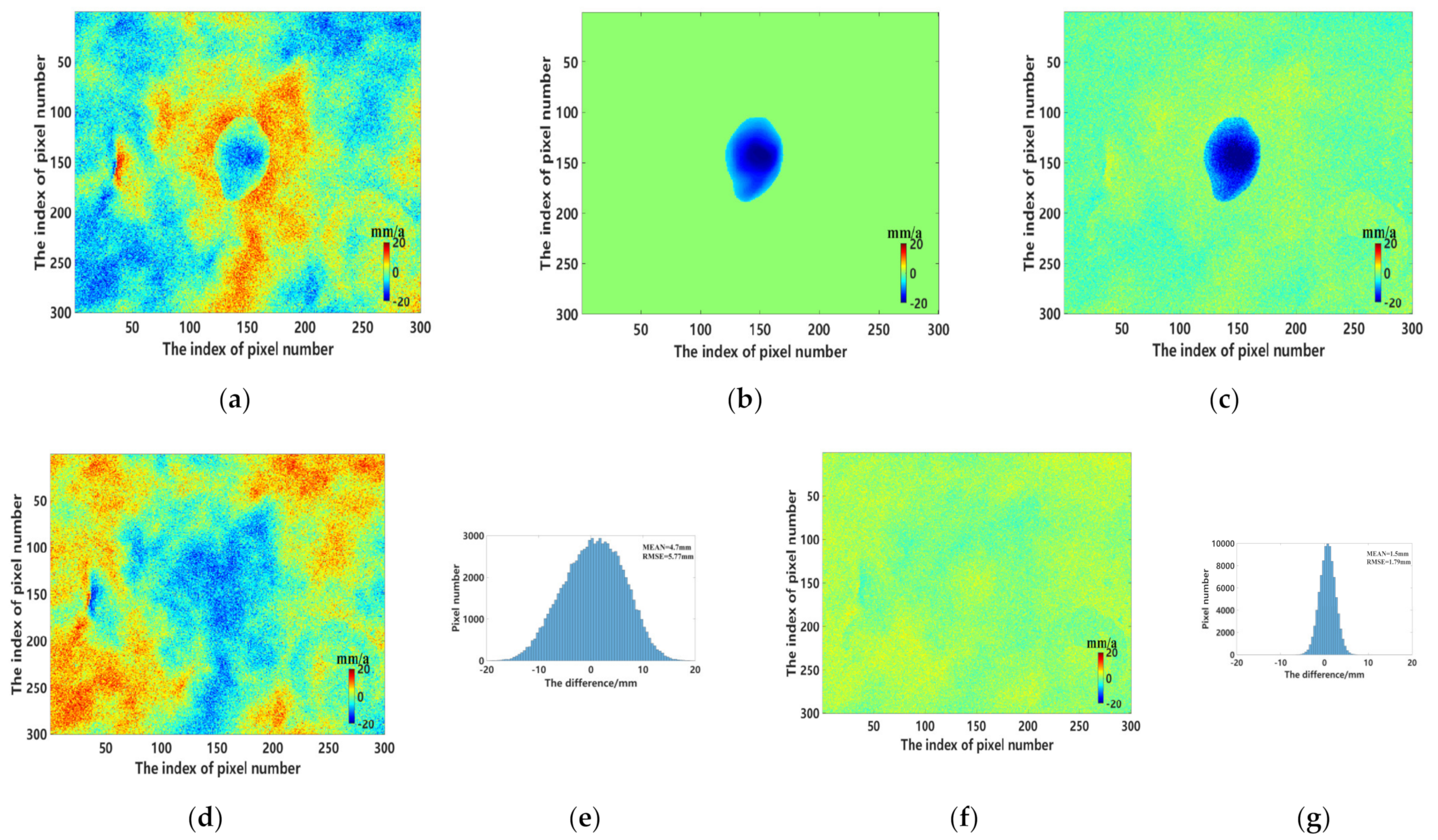
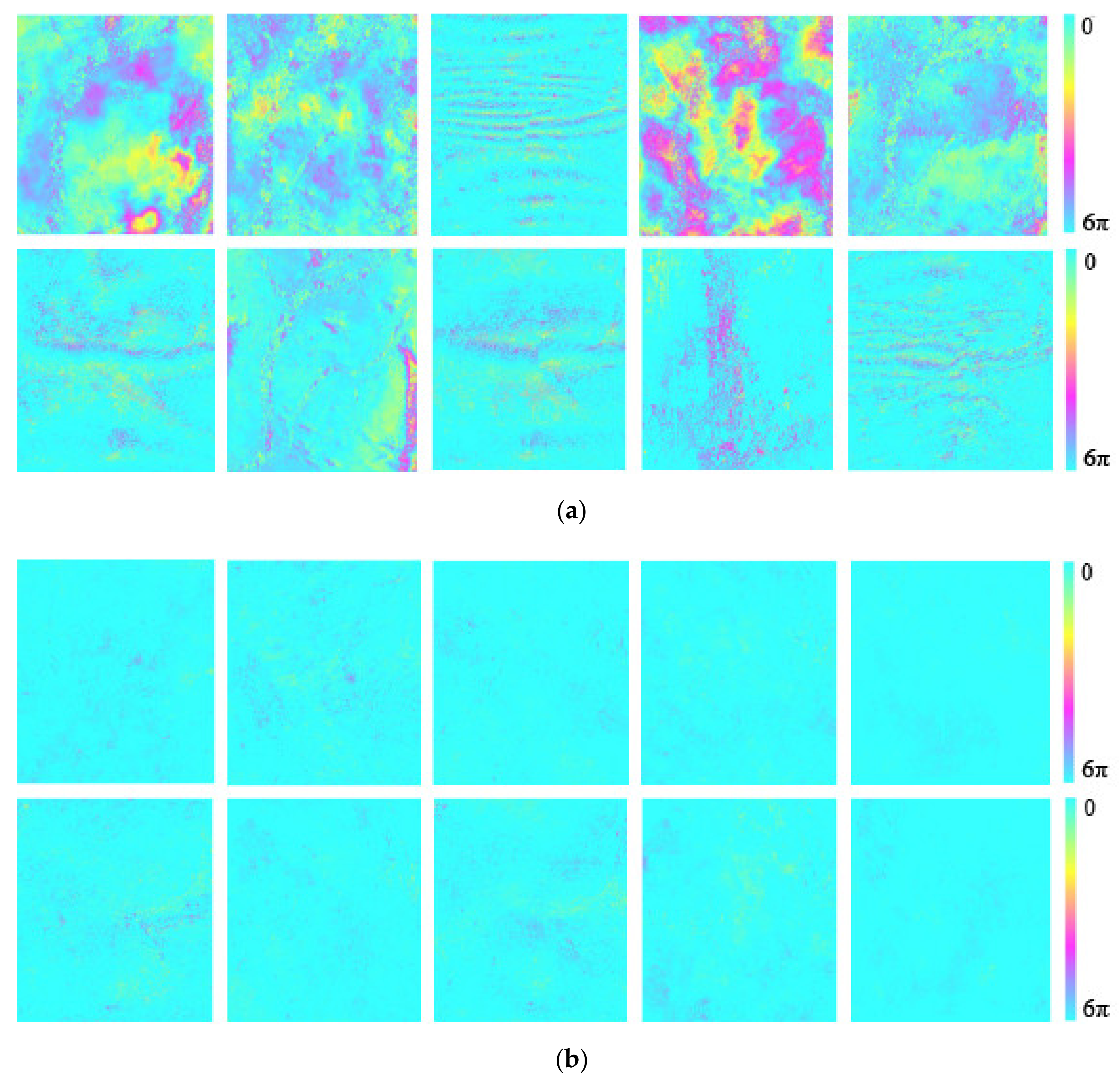
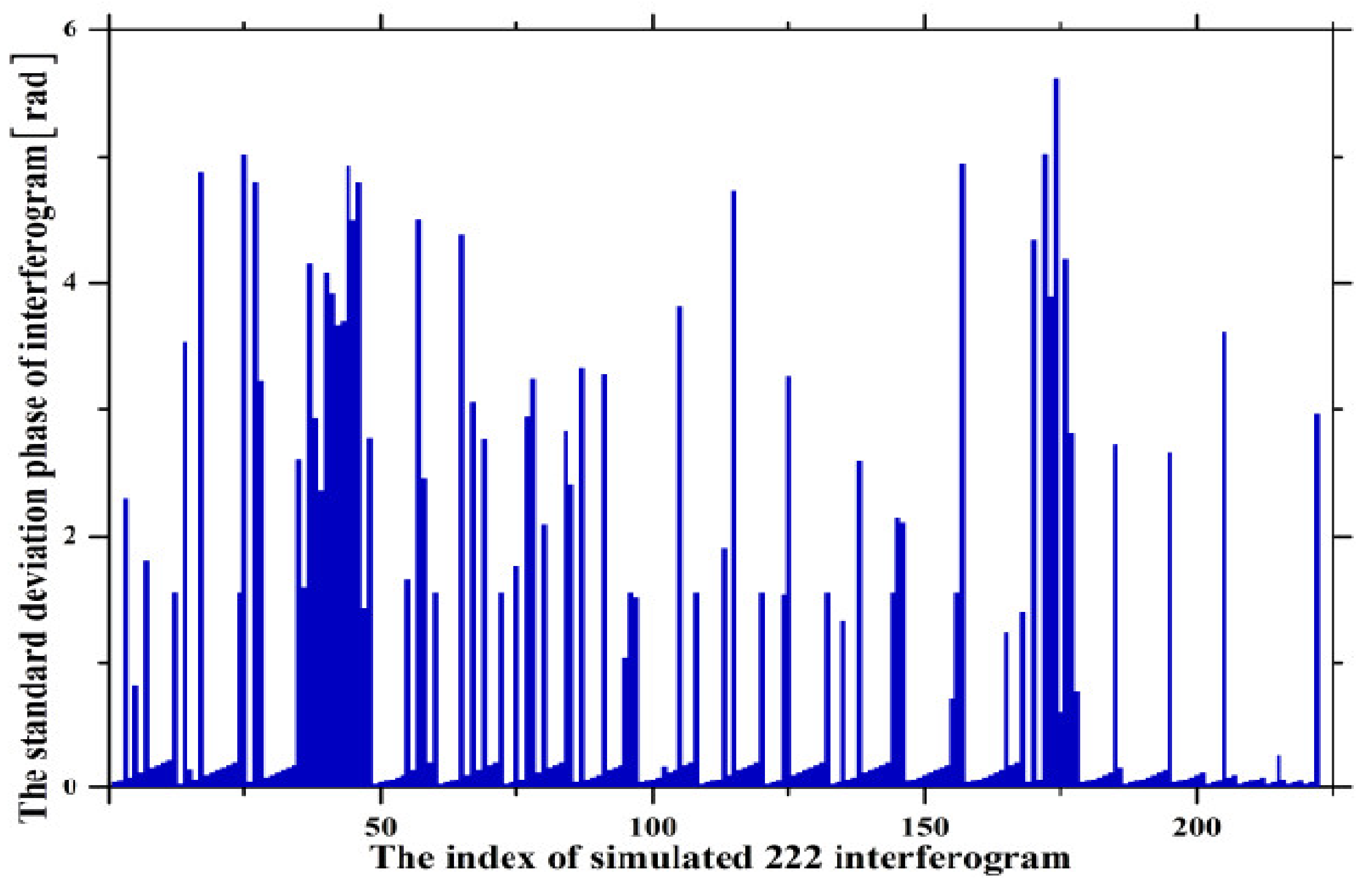
3.1. Simulation-Based Tests
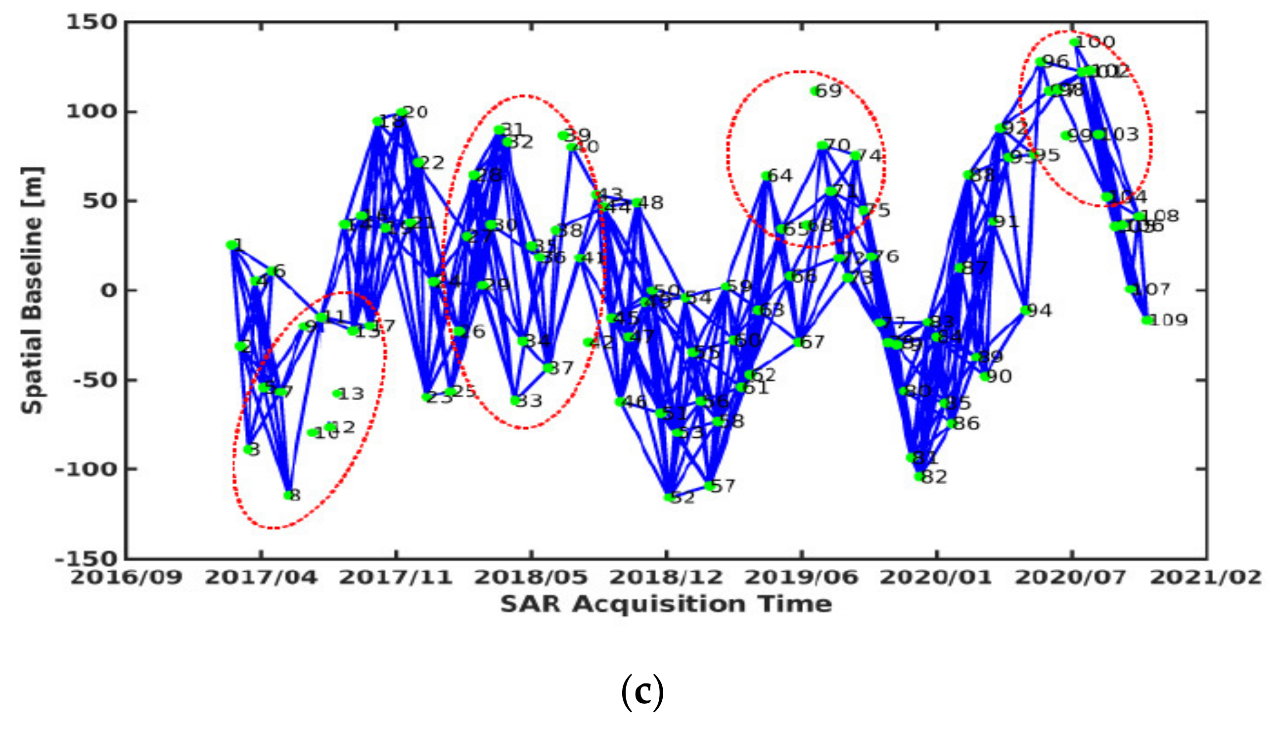
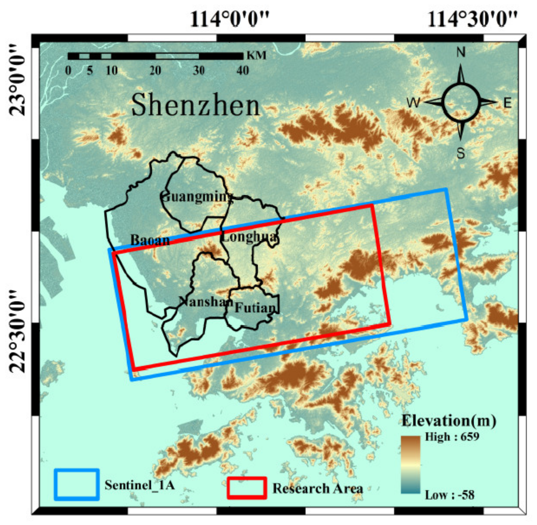
3.2. Actual Subsidence Issues
4. Conclusions
Author Contributions
Funding
Institutional Review Board Statement
Informed Consent Statement
Data Availability Statement
Acknowledgments
Conflicts of Interest
References
- Zhang, B.; Xu, G.; Lu, Z.; He, Y.; Peng, M.; Feng, X. Coseismic Deformation Mechanisms of the 2021 Ms 6.4 Yangbi Earthquake, Yunnan Province, Using InSAR Observations. Remote Sens. 2021, 13, 3961. [Google Scholar] [CrossRef]
- Casu, F.; Manzo, M.; Lanari, R. A quantitative assessment of the SBAS algorithm performance for surface deformation retrieval from DInSAR data. Remote Sens. Environ. 2006, 102, 195–210. [Google Scholar] [CrossRef]
- Hooper, A.; Bekaert, D.; Spaans, K.; Arıkan, M. Recent advances in SAR interferometry time series analysis for measuring crustal deformation. Tectonophysics 2012, 514–517, 1–13. [Google Scholar] [CrossRef]
- Berardino, P.; Fornaro, G.; Lanari, R.; Sansosti, E. A new algorithm for surface deformation monitoring based on small baseline differential SAR interferograms. IEEE Trans. Geosci. Remote Sens. 2002, 40, 2375–2383. [Google Scholar] [CrossRef] [Green Version]
- Tizzani, P.; Berardino, P.; Casu, F.; Euillades, P.; Manzo, M.; Ricciardi, G.P.; Zeni, G.; Lanari, R. Surface deformation of Long Valley caldera and Mono Basin, California, investigated with the SBAS-InSAR approach. Remote Sens. Environ. 2007, 108, 277–289. [Google Scholar] [CrossRef]
- Zhao, F.; Meng, X.; Zhang, Y.; Chen, G.; Su, X.; Yue, D. Landslide Susceptibility Mapping of Karakorum Highway Combined with the Application of SBAS-InSAR Technology. Sensors 2019, 19, 2685. [Google Scholar] [CrossRef] [Green Version]
- Teshebaeva, K.; Roessner, S.; Echtler, H.; Motagh, M.; Wetzel, H.-U.; Molodbekov, B. ALOS/PALSAR InSAR Time-Series Analysis for Detecting Very Slow-Moving Landslides in Southern Kyrgyzstan. Remote Sens. 2015, 7, 8973–8994. [Google Scholar] [CrossRef] [Green Version]
- Liu, D.; Shao, Y.; Liu, Z.; Riedel, B.; Sowter, A.; Niemeier, W.; Bian, Z. Evaluation of InSAR and TomoSAR for Monitoring Deformations Caused by Mining in a Mountainous Area with High Resolution Satellite-Based SAR. Remote Sens. 2014, 6, 1476–1495. [Google Scholar] [CrossRef] [Green Version]
- Raspini, F.; Bianchini, S.; Ciampalini, A.; Del Soldato, M.; Solari, L.; Novali, F.; Del Conte, S.; Rucci, A.; Ferretti, A.; Casagli, N. Continuous, semi-automatic monitoring of ground deformation using Sentinel-1 satellites. Sci. Rep. 2018, 8, 7253. [Google Scholar] [CrossRef] [Green Version]
- Hu, B.; Wang, H.S.; Sun, Y.L.; Hou, J.G.; Liang, J. Long-Term Land Subsidence Monitoring of Beijing (China) Using the Small Baseline Subset (SBAS) Technique. Remote Sens. 2014, 6, 3648–3661. [Google Scholar] [CrossRef] [Green Version]
- Casu, F.; Lanari, R.; Sansosti, E.; Poland, M.; Miklius, A.; Solaro, G.; Tizzani, P. SBAS-InSAR analysis of surface deformation at Mauna Loa and Kilauea volcanoes in Hawaii. In Proceedings of the 2009 IEEE International Geoscience and Remote Sensing Symposium, Cape Town, South Africa, 12–17 July 2009; pp. IV-41–IV-44. [Google Scholar]
- Mouginot, J.; Scheuchl, B.; Rignot, E. Mapping of Ice Motion in Antarctica Using Synthetic-Aperture Radar Data. Remote Sens. 2012, 4, 2753–2767. [Google Scholar] [CrossRef] [Green Version]
- Zhang, L.; Lu, Z.; Ding, X.; Jung, H.-S.; Feng, G.; Lee, C.-W. Mapping ground surface deformation using temporarily coherent point SAR interferometry: Application to Los Angeles Basin. Remote Sens. Environ. 2012, 117, 429–439. [Google Scholar] [CrossRef]
- Zhang, Y.; Zhang, J.; Gong, W.; Lu, Z. Monitoring urban subsidence based on SAR lnterferometric point target analysis. Acta Geod. Cartogr. Sin. 2009, 38, 482–487. [Google Scholar]
- Casu, F.; Manconi, A.; Pepe, A.; Lanari, R. Deformation Time-Series Generation in Areas Characterized by Large Displacement Dynamics: The SAR Amplitude Pixel-Offset SBAS Technique. IEEE Trans. Geosci. Remote Sens. 2011, 49, 2752–2763. [Google Scholar] [CrossRef]
- Esfahany, S.S. Exploitation of Distributed Scatterers in Synthetic Aperture Radar Interferometry. Ph.D. Thesis, Delft University of Technology, Delft, The Netherlands, March 2017. [Google Scholar]
- Agram, P.S.; Simons, M. A noise model for InSAR time series. J. Geophys. Res. Solid Earth JGR 2015, 120, 2752–2771. [Google Scholar] [CrossRef]
- Cao, Y.; Li, Z.; Wei, J.; Hu, J.; Duan, M.; Feng, G. Stochastic modeling for time series InSAR: With emphasis on atmospheric effects. J. Geod. 2018, 92, 185–204. [Google Scholar] [CrossRef]
- Jiang, M.; Guarnieri, A.M. Distributed Scatterer Interferometry With the Refinement of Spatiotemporal Coherence. IEEE Trans. Geosci. Remote Sens. 2020, 58, 3977–3987. [Google Scholar] [CrossRef]
- Wang, Z.; Zhang, J.; Yu, Y.; Liu, J.; Liu, W.; Jiang, N.; Guo, D. Monitoring, Analyzing, and Modeling for Single Subsidence Basin in Coal Mining Areas Based on SAR Interferometry with L-Band Data. Sci. Program. 2021, 2021, 6662097. [Google Scholar] [CrossRef]
- Pepe, A.; Yang, Y.; Manzo, M.; Lanari, R. Improved EMCF-SBAS Processing Chain Based on Advanced Techniques for the Noise-Filtering and Selection of Small Baseline Multi-Look DInSAR Interferograms. IEEE Trans. Geosci. Remote Sens. 2015, 53, 4394–4417. [Google Scholar] [CrossRef]
- Duan, M.; Xu, B.; Li, Z.; Wu, W.; Wei, J.; Cao, Y.; Liu, J. Adaptively Selecting Interferograms for SBAS-InSAR Based on Graph Theory and Turbulence Atmosphere. IEEE Access 2020, 8, 112898–112909. [Google Scholar] [CrossRef]
- Casu, F.; Manunta, M.; Agram, P.S.; Crippen, R.E. Big Remotely Sensed Data: Tools, applications and experiences. Remote Sens. Environ. 2017, 202, 1–2. [Google Scholar] [CrossRef]
- Krizhevsky, A.; Sutskever, I.; Hinton, G.E. ImageNet classification with deep convolutional neural networks. Commun. ACM 2017, 60, 84–90. [Google Scholar] [CrossRef]
- Smirnov, E.A.; Timoshenko, D.M.; Andrianov, S.N. Comparison of Regularization Methods for ImageNet Classification with Deep Convolutional Neural Networks. AASRI Procedia 2014, 6, 89–94. [Google Scholar] [CrossRef]
- Mukherjee, S.; Zimmer, A.; Sun, X.; Ghuman, P.; Cheng, I. An Unsupervised Generative Neural Approach for InSAR Phase Filtering and Coherence Estimation. IEEE Geosci. Remote Sens. Lett. 2020, 18, 1971–1975. [Google Scholar] [CrossRef]
- Ouahabi, A.; Taleb-Ahmed, A. Deep learning for real-time semantic segmentation: Application in ultrasound imaging. Pattern Recognit. Lett. 2021, 144, 27–34. [Google Scholar] [CrossRef]
- Khaldi, Y.; Benzaoui, A.; Ouahabi, A.; Jacques, S.; Taleb-Ahmed, A. Ear Recognition Based on Deep Unsupervised Active Learning. IEEE Sens. J. 2021, 21, 20704–20713. [Google Scholar] [CrossRef]
- Adjabi, I.; Ouahabi, A.; Benzaoui, A.; Jacques, S. Multi-Block Color-Binarized Statistical Images for Single-Sample Face Recognition. Sensors 2021, 21, 728. [Google Scholar] [CrossRef]
- Adjabi, I.; Ouahabi, A.; Benzaoui, A.; Taleb-Ahmed, A. Past, Present, and Future of Face Recognition: A Review. Electronics 2020, 9, 1188. [Google Scholar] [CrossRef]
- Anantrasirichai, N.; Biggs, J.; Kelevitz, K.; Sadeghi, Z.; Bull, D. Deep Learning Framework for Detecting Ground Deformation in the Built Environment using Satellite InSAR data. IEEE Trans. Geosci. Remote Sens. 2020, 59, 2940–2950. [Google Scholar] [CrossRef]
- Abrams, J.F.; Vashishtha, A.; Wong, S.T.; Nguyen, A.; Mohamed, A.; Wieser, S.; Kuijper, A.; Wilting, A.; Mukhopadhyay, A. Habitat-Net: Segmentation of habitat images using deep learning. Ecol. Inform. 2019, 51, 121–128. [Google Scholar] [CrossRef]
- Sun, J.; Wauthier, C.; Stephens, K.; Gervais, M.; Cervone, G.; La Femina, P.; Higgins, M. Automatic Detection of Volcanic Surface Deformation Using Deep Learning. J. Geophys. Res. Solid Earth 2020, 125, e2020JB019840. [Google Scholar] [CrossRef]
- Yilmaz, I. Landslide susceptibility mapping using frequency ratio, logistic regression, artificial neural networks and their comparison: A case study from Kat landslides (Tokat—Turkey). Comput. Geosci. 2009, 35, 1125–1138. [Google Scholar] [CrossRef]
- He, K.; Zhang, X.; Ren, S.; Sun, J. Identity Mappings in Deep Residual Networks. In Proceedings of the Computer Vision—ECCV 2016, Amsterdam, The Netherlands, 11–14 October 2016; pp. 630–645. [Google Scholar]
- Szegedy, C.; Ioffe, S.; Vanhoucke, V.; Alemi, A. Inception-v4, Inception-ResNet and the Impact of Residual Connections on Learning. Available online: https://arxiv.org/abs/1602.07261 (accessed on 25 October 2021).
- Graupe, D. Deep Learning Neural Networks; Elsevier Science Ltd.: Amsterdam, The Netherlands, 2015; Volume 61, pp. 85–117. [Google Scholar] [CrossRef] [Green Version]
- Chen, Y.; Lin, Z.; Zhao, X.; Wang, G.; Gu, Y. Deep Learning-Based Classification of Hyperspectral Data. IEEE J. Sel. Top. Appl. Earth Obs. Remote Sens. 2014, 7, 2094–2107. [Google Scholar] [CrossRef]
- Hamiane, M.; Jacques, S.; Ouahabi, A.; Arbaoui, A. Wavelet-based multiresolution analysis coupled with deep learning to efficiently monitor cracks in concrete. Frat. Integrità Strutt. 2021, 15, 33–47. [Google Scholar] [CrossRef]
- Arbaoui, A.; Ouahabi, A.; Jacques, S.; Hamiane, M. Concrete Cracks Detection and Monitoring Using Deep Learning-Based Multiresolution Analysis. Electronics 2021, 10, 1772. [Google Scholar] [CrossRef]
- Guzzetti, F.; Manunta, M.; Ardizzone, F.; Pepe, A.; Cardinali, M.; Zeni, G.; Reichenbach, P.; Lanari, R. Analysis of Ground Deformation Detected Using the SBAS-DInSAR Technique in Umbria, Central Italy. Pure Appl. Geophys. 2009, 166, 1425–1459. [Google Scholar] [CrossRef]
- Gee, D.; Bateson, L.; Sowter, A.; Grebby, S.; Novellino, A.; Cigna, F.; Marsh, S.; Banton, C.; Wyatt, L. Ground Motion in Areas of Abandoned Mining: Application of the Intermittent SBAS (ISBAS) to the Northumberland and Durham Coalfield, UK. Geosciences 2017, 7, 85. [Google Scholar] [CrossRef] [Green Version]
- Goyal, P.; Dollár, P.; Girshick, R.; Noordhuis, P.; Wesolowski, L.; Kyrola, A.; Tulloch, A.; Jia, Y.; He, K. Accurate, Large Minibatch SGD: Training ImageNet in 1 Hour. arXiv 2017, arXiv:1706.02677. [Google Scholar]
- Cao, Q.; Shen, L.; Xie, W.; Parkhi, O.M.; Zisserman, A. VGGFace2: A Dataset for Recognising Faces across Pose and Age. In Proceedings of the 2018 13th IEEE International Conference on Automatic Face & Gesture Recognition (FG 2018), Xi’an, China, 15–19 May 2018; pp. 67–74. [Google Scholar]
- Tzirakis, P.; Trigeorgis, G.; Nicolaou, M.A.; Schuller, B.W.; Zafeiriou, S. End-to-End Multimodal Emotion Recognition Using Deep Neural Networks. IEEE J. Sel. Top. Signal Process. 2017, 11, 1301–1309. [Google Scholar] [CrossRef] [Green Version]
- Bruzzone, L.; Prieto, D.F.; Serpico, S.B. A neural-statistical approach to multitemporal and multisource remote-sensing image classification. IEEE Trans. Geosci. Remote Sens. 1999, 37, 1350–1359. [Google Scholar] [CrossRef] [Green Version]
- Kuncheva, L.I. Combining Classiers: Soft Computing Solutions; World Scientific: Singapore, 2001. [Google Scholar]
- Labat, V.; Remenieras, J.P.; Bou Matar, O.; Ouahabi, A.; Patat, F. Harmonic propagation of finite amplitude sound beams: Experimental determination of the nonlinearity parameter B/A. Ultrasonics 2000, 38, 292–296. [Google Scholar] [CrossRef]
- Ouahabi, A. A review of wavelet denoising in medical imaging. In Proceedings of the 2013 8th International Workshop on Systems, Signal Processing and Their Applications (WoSSPA), Algiers, Algeria, 12–15 May 2013; pp. 19–26. [Google Scholar]
- Ahmed, S.S.; Messali, Z.; Ouahabi, A.; Trepout, S.; Messaoudi, C.; Marco, S. Nonparametric Denoising Methods Based on Contourlet Transform with Sharp Frequency Localization: Application to Low Exposure Time Electron Microscopy Images. Entropy 2015, 17, 3461–3478. [Google Scholar] [CrossRef] [Green Version]
- Hanssen, R.F. Radar Interferometry Data Interpretation and Error Analysis; Springer Science & Business Media: Berlin/Heidelberg, Germany, 2001. [Google Scholar]
- Santoro, M.; Wegmuller, U.; Askne, J.I.H. Signatures of ERS–Envisat Interferometric SAR Coherence and Phase of Short Vegetation: An Analysis in the Case of Maize Fields. IEEE Trans. Geosci. Remote Sens. 2010, 48, 1702–1713. [Google Scholar] [CrossRef]
- Lee, C.-W.; Lu, Z.; Jung, H.-S. Simulation of time-series surface deformation to validate a multi-interferogram InSAR processing technique. Int. J. Remote Sens. 2012, 33, 7075–7087. [Google Scholar] [CrossRef]
- Xu, B.; Feng, G.; Li, Z.; Wang, Q.; Wang, C.; Xie, R. Coastal Subsidence Monitoring Associated with Land Reclamation Using the Point Target Based SBAS-InSAR Method: A Case Study of Shenzhen, China. Remote Sens. 2016, 8, 652. [Google Scholar] [CrossRef] [Green Version]
- Liu, P.; Chen, X.; Li, Z.; Zhang, Z.; Xu, J.; Feng, W.; Wang, C.; Hu, Z.; Tu, W.; Li, H. Resolving Surface Displacements in Shenzhen of China from Time Series InSAR. Remote Sens. 2018, 10, 1162. [Google Scholar] [CrossRef] [Green Version]
- He, Y.; Xu, G.; Kaufmann, H.; Wang, J.; Ma, H.; Liu, T. Integration of InSAR and LiDAR Technologies for a Detailed Urban Subsidence and Hazard Assessment in Shenzhen, China. Remote Sens. 2021, 13, 2366. [Google Scholar] [CrossRef]
- Zhao, Q.; Lin, H.; Chen, F.; Gao, W. InSAR detection of residual settlement of ocean reclamation areas in Shenzhen, China. In Proceedings of the 2011 19th International Conference on Geoinformatics, Shanghai, China, 24–26 June 2011; pp. 1–5. [Google Scholar]
- Lu, D.; Toro, F.G.; Cai, B. Methods for certification of GNSS-based safe vehicle localisation i. In Proceedings of the IEEE 2015 International Conference on Connected Vehicles and Expo (ICCVE), Shenzhen, China, 19–23 October 2015; pp. 226–231. [Google Scholar]


| Layer Name | Output Size | Configuration |
|---|---|---|
| CONV_1 | 1/2 | 77, 64, stride = 2 |
| CONV_2 | 1/4 | |
| CONV_3 | 1/8 | |
| CONV_4 | 1/16 | |
| CONV_5 | 1/32 | |
| Classifier | 11 | Average pooling, Fc (Full connection), 1000, Softmax |
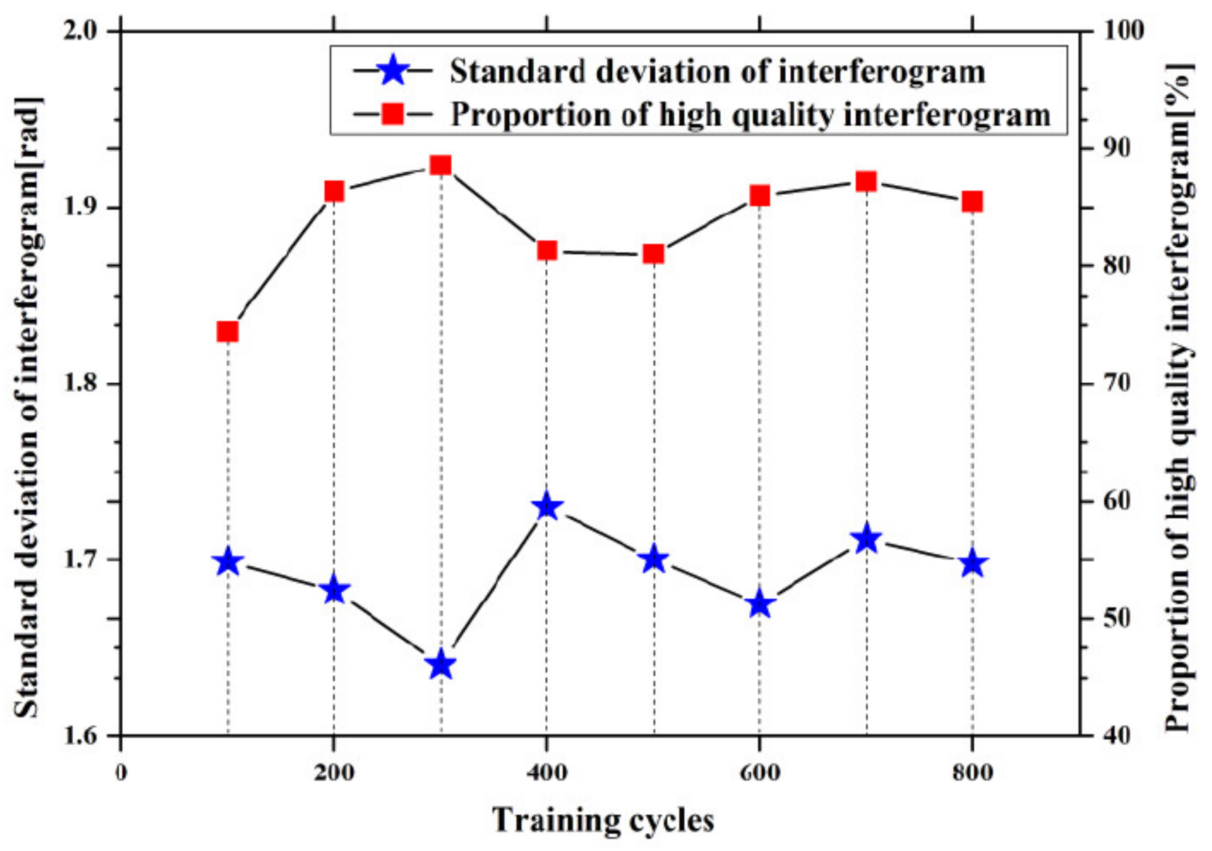
| Size of Input Image | Training Cycles | Interferogram Number | Standard Deviation of Interferogram Phase/Rad | Accuracy (%) |
|---|---|---|---|---|
| 128 × 128 | 100 | 432 | 1.699 | 74.4 |
| 128 × 128 | 200 | 447 | 1.6829 | 86.34 |
| 128 × 128 | 300 | 425 | 1.6406 | 88.53 |
| 128 × 128 | 400 | 461 | 1.7302 | 81.28 |
| 128 × 128 | 500 | 431 | 1.7005 | 80.10 |
| 128 × 128 | 600 | 441 | 1.6749 | 86.00 |
| 128 × 128 | 700 | 464 | 1.7118 | 87.18 |
| 128 × 128 | 800 | 456 | 1.6982 | 85.50 |
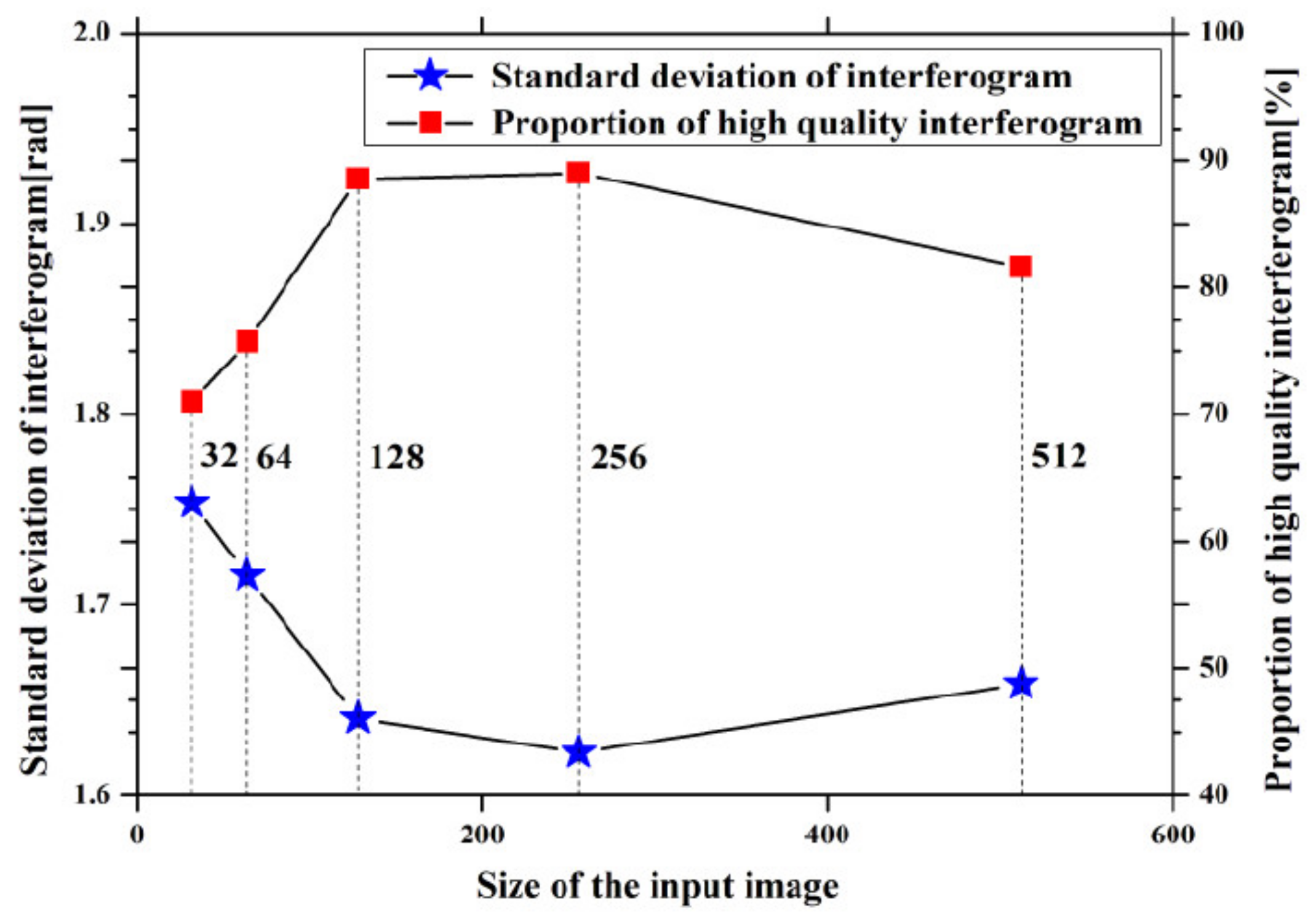
| 32 × 32 | 300 | 437 | 1.7537 | 71.0 |
| 64 × 64 | 300 | 448 | 1.7153 | 75.71 |
| 128 × 128 | 300 | 425 | 1.6406 | 88.53 |
| 256 × 256 | 300 | 414 | 1.6225 | 89.00 |
| 512 × 512 | 300 | 411 | 1.6585 | 81.62 |
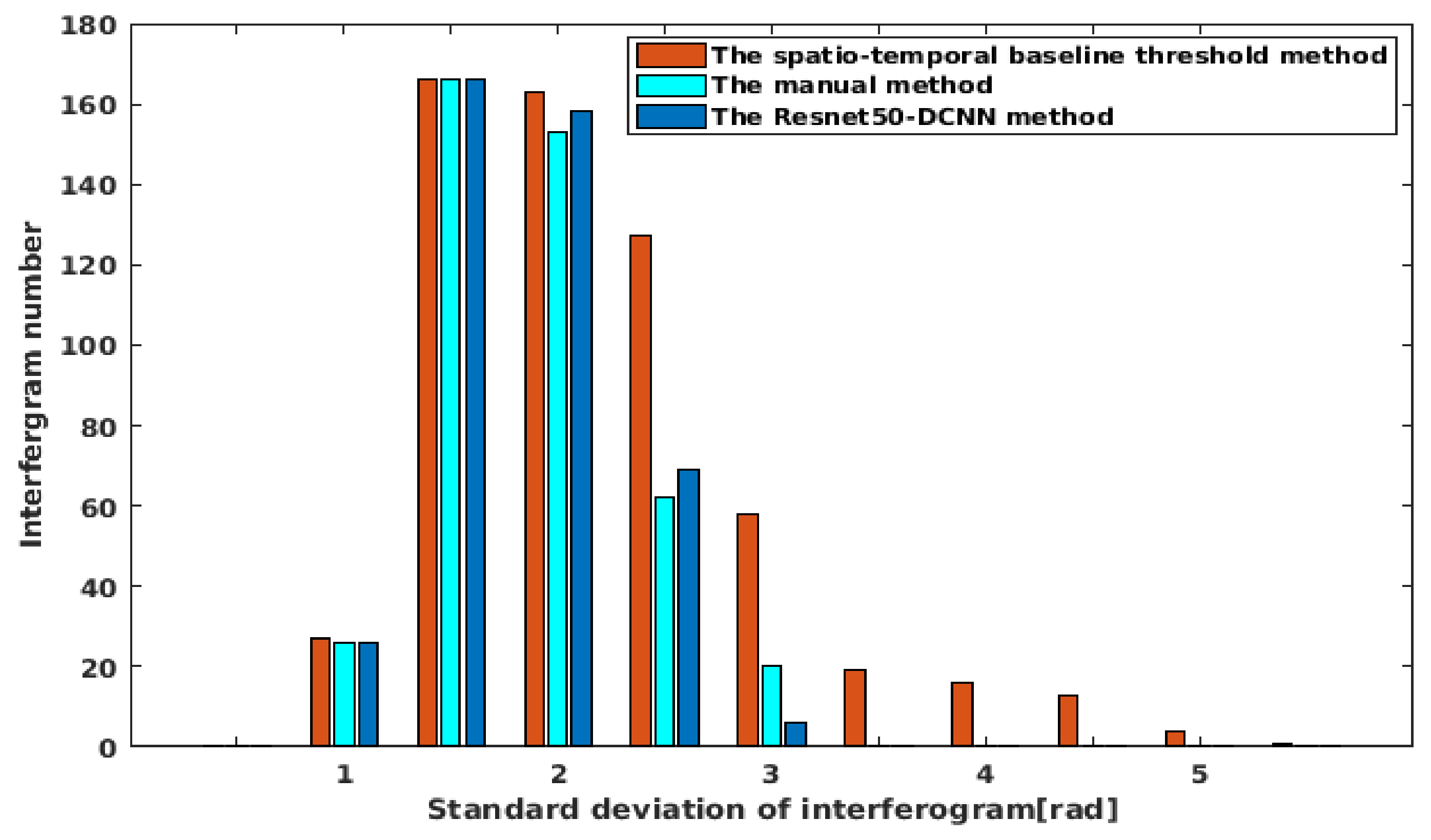
| The Spatio–Temporal Baseline Threshold Method | The Manual Method | The ResNet50–DCNN Method | |
|---|---|---|---|
| Number of interferogram | 593 | 411 | 425 |
| Standard deviation of interferogram phase/rad | 2.1054 | 1.6328 | 1.6406 |
Publisher’s Note: MDPI stays neutral with regard to jurisdictional claims in published maps and institutional affiliations. |
© 2021 by the authors. Licensee MDPI, Basel, Switzerland. This article is an open access article distributed under the terms and conditions of the Creative Commons Attribution (CC BY) license (https://creativecommons.org/licenses/by/4.0/).
Share and Cite
He, Y.; Zhang, G.; Kaufmann, H.; Xu, G. Automatic Interferogram Selection for SBAS-InSAR Based on Deep Convolutional Neural Networks. Remote Sens. 2021, 13, 4468. https://doi.org/10.3390/rs13214468
He Y, Zhang G, Kaufmann H, Xu G. Automatic Interferogram Selection for SBAS-InSAR Based on Deep Convolutional Neural Networks. Remote Sensing. 2021; 13(21):4468. https://doi.org/10.3390/rs13214468
Chicago/Turabian StyleHe, Yufang, Guangzong Zhang, Hermann Kaufmann, and Guochang Xu. 2021. "Automatic Interferogram Selection for SBAS-InSAR Based on Deep Convolutional Neural Networks" Remote Sensing 13, no. 21: 4468. https://doi.org/10.3390/rs13214468
APA StyleHe, Y., Zhang, G., Kaufmann, H., & Xu, G. (2021). Automatic Interferogram Selection for SBAS-InSAR Based on Deep Convolutional Neural Networks. Remote Sensing, 13(21), 4468. https://doi.org/10.3390/rs13214468