Article

A Preliminary Assessment of a Newly-Defined Multispectral Hue Space for Retrieving River Depth with Optical Imagery and In Situ Calibration Data

Sorbonne Université, CNRS, EPHE, UMR 7619 METIS, 4 Place Jussieu, Box 105, 75005 Paris, France
*
Author to whom correspondence should be addressed.
Remote Sens. 2021, 13(21), 4435; https://doi.org/10.3390/rs13214435
Submission received: 21 September 2021 / Revised: 29 October 2021 / Accepted: 29 October 2021 / Published: 4 November 2021

Abstract

:
Bathymetry is a key element in the modeling of river systems for flood mapping, geomorphology, or stream habitat characterization. Standard practices rely on the interpolation of in situ depth measurements obtained with differential GPS or total station surveys, while more advanced techniques involve bathymetric LiDAR or acoustic soundings. However, these high-resolution active techniques are not so easily applied over large areas. Alternative methods using passive optical imagery present an interesting trade-off: they rely on the fact that wavelengths composing solar radiation are not attenuated at the same rates in water. Under certain assumptions, the logarithm of the ratio of radiances in two spectral bands is linearly correlated with depth. In this study, we go beyond these ratio methods in defining a multispectral hue that retains all spectral information. Given n coregistered bands, this spectral invariant lies on the ( n 2 ) -sphere embedded in R n 1 , denoted S n 2 and tagged ‘hue hypersphere’. It can be seen as a generalization of the RGB ‘color wheel’ ( S 1 ) in higher dimensions. We use this mapping to identify a hue-depth relation in a 35 km reach of the Garonne River, using high resolution (0.50 m) airborne imagery in four bands and data from 120 surveyed cross-sections. The distribution of multispectral hue over river pixels is modeled as a mixture of two components: one component represents the distribution of substrate hue, while the other represents the distribution of ‘deep water’ hue; parameters are fitted such that membership probability for the ‘deep’ component correlates with depth.

Graphical Abstract

1. Introduction

Characterizing river channel bathymetry by average parameters (e.g., average depth, cross-section area, hydraulic radius) or sparsely distributed cross-sections may be sufficient for certain applications; however, a precise description is needed for applications in geomorphology or ecology, where local flow parameters are known to vary at the scale of a few times the full bank width in the streamwise direction with alternating morphological units such as pools, runs, and riffles [1,2].
Dense and precise bathymetric survey requires active measurement techniques such as bathymetric LiDAR using water-penetrating wavelengths in the visible spectrum [3,4], or acoustic soundings [5]. Unfortunately, these techniques rely on an artificial illuminating source (either electromagnetic or acoustic) and thus have a high operating cost and are very difficult to use over large areas.
A very interesting alternative is offered by passive optical methods, which have been used in marine, coastal, and more recently river settings since the pioneering work of Lyzenga [6]. Here, natural sunlight is the illuminating source and depth is retrieved by analyzing the radiance signal received at the sensor. According to Marcus and Fonstad [7], this simple method may actually be ‘the only viable method for measuring, monitoring and mapping a large suite of in-channel river parameters continuously at sub-meter resolution’.
Following this introduction, Section 2 of this paper will provide a quick overview of the principles behind remotely-sensed estimation of river bathymetry using spectral ratios between bands in multispectral images. Then, in Section 3, we will temporarily move away from this specific application and propose a formal definition of a more general multispectral hue. Our procedure for estimating depth using this multispectral hue will be the core of Section 4, and results will be presented in Section 5. Then, we will summarize our findings and propose perspectives in Section 6.

2. Principles of Remotely-Sensed Estimation of River Bathymetry Using Passive Optical Measurements

As illustrated in Figure 1, the total upwelling spectral radiance (in W·m−2·sr−1) over water in a given spectral band with central wavelength λ can be split into four components (e.g., Legleiter et al. [8]):
L ( λ ) = L b ( λ ) + L c ( λ ) + L s ( λ ) + L p ( λ )
  • L b is the radiance originating from the Lambertian (diffuse) reflection from the bed substrate;
  • L c is the volume radiance of the water column of depth h, which is basically sunlight that has been backscattered upwards before reaching the bottom;
  • L s is the surface radiance due to specular reflections at the air–water interface. L s can make up a large fraction of L for certain geometries or viewing angles (‘sun glints’);
  • L p is a path radiance due to atmospheric scattering.
Providing that we can account for both atmospheric path radiance and surface radiance, Philpot [10] derived the following expression for the total radiance measured at a given pixel of the sensor:
L ( x , λ ) L b ( x , λ ) + L c ( x , λ ) R b ( x , λ ) R c , ( λ ) e K ( λ ) h ( x ) + R c , ( λ ) R mix ( x , h , λ ) mixture reflectance C 0 T a ( λ ) E ( λ )
The rightmost term E ( λ ) is the downwelling solar irradiance in the spectral band (in W·m−2), while the product C 0 T a (in sr−1) accounts for both atmospheric and air–water interface transmission ( C 0 can be considered roughly independent of wavelength). These terms are then multiplied by a reflectance term (brackets) which, according to Philpot, can be written as a mixture between two ‘end-members’:
  • The first end-member is the reflectance of bed/substrate, R b , which depends on both location x and wavelength λ ,
  • The second end-member is the reflectance R c , that would be measured over an ‘infinitely deep’ water column.
The weight of the bed reflectance R b in the mixture reflectance R mix is an exponentially decreasing function of depth, with an attenuation coefficient K ( λ ) , which depends on the wavelength (Beer–Lambert law).
While the solar irradiance E ( λ ) depends on the time of the day and on cloudiness, taking the ratio of solar irradiances in two different spectral bands cancels these variations. Hence, it is convenient to take the ratio:
L ( x , λ i ) L ( x , λ j ) = R b ( x , λ i ) R c , ( λ i ) e K ( λ i ) h ( x ) + R c , ( λ i ) R b ( x , λ j ) R c , ( λ j ) e K ( λ j ) h ( x ) + R c , ( λ j ) C 0 T a ( λ i ) E ( λ i ) C 0 T a ( λ j ) E ( λ j )
Two common assumptions are then made to proceed with this expression:
  • First, the reflectance R c , of deep water is assumed to be small compared to the bed reflectance R b (for any substrate and any wavelength). Deep water reflectance is certainly low if the water is clear, but this assumption breaks down in the presence of sediment, dissolved organic matter, algae, etc. Furthermore, the bed might have a very low reflectance. Quartz sand might be highly reflective, but mud and rocks (especially rocks coated with a microbial film) can be quite dark;
  • Second, the ratio of bed reflectances at wavelengths λ i and λ j , R b ( x , λ i ) R b ( x , λ j ) is approximated as uniform in space.
With these assumptions, Equation (3) can be simplified and boils down to a linear relationship between depth and the logarithm of the spectral ratio:
X i j = ln L ( x , λ i ) L ( x , λ j ) K ( λ j ) K ( λ i ) slope ( λ i , λ j ) h + ln R b ( λ i ) R b ( λ j ) + ln C 0 T a ( λ i ) E ( λ i ) C 0 T a ( λ j ) E ( λ j ) intercept ( λ i , λ j )
Slope and intercept depend on optical properties of the atmosphere, water, and substrate at each wavelength but, if they can be considered invariant across the image, Equation (4) provides a predictor for depth. It has been used in numerous studies (see Shah et al. [11] for a recent review), either with the calibration of slope and intercept against in situ depth measurement, or without calibration; in the latter case, attenuation coefficients K ( λ ) have to be modeled physically [12,13].
For a multispectral image with n coregistered bands, n ( n 1 ) spectral ratios can be computed, but only ( n 1 ) are independent (keeping those between adjacent bands for instance) since
X i k = ln L ( λ i ) L ( λ k ) = ln L ( λ i ) L ( λ j ) L ( λ j ) L ( λ k ) = X i j + X j k
Hence, a ratio–depth relation can be obtained by identifying a single, optimal pair of bands [8], or using several log-transformed ratios given by several pairs [14]. The use of multiple ratios (or other predictors) will increase model flexibility, though attention must be paid to multicollinearity [15]. In fact, retaining all spectral information from the ( n 1 ) independent ratios amounts to defining a multispectral ‘hue’, or ‘pure color’, independent of illumination conditions. The definition of such a spectral invariant is presented in Section 3.

3. Beyond Spectral Ratios: A Definition of Multispectral Hue

3.1. Rationale for the Definition of Multispectral Hue

3.1.1. RGB Case: The Color Wheel

Let us start with an example that will be familiar to many: many computer programs offer a color definition tool that relies on the kind of ‘color wheel’ shown in Figure 2. In this tool, a hue or ‘pure color’ can be selected along a circle, with an angle ranging between 0 and 360°. Two other operations can then be performed to obtain the final red, green and blue components:
  • The pure color can be partially desaturated, i.e., mixed with a white component. Such a mixing can occur for example with specular reflections, which will appear nearly white under white illumination if the refractive index of the material is slowly varying with wavelength (this is the case for water, or for an object coated with varnish).
  • The overall brightness or value of the color can be decreased. Physically speaking, this other operation is similar to either reducing the intensity of the light source, or changing the orientation of an object’s surface normals so that less light is diffused towards the sensor (‘shaded face’ effect).

3.1.2. Notations

In this section and the following ones, we will use bold symbols to denote points, vectors or matrices in a multidimensional space. Denoting v T the transpose of v , [ 1 , 1 , 1 ] denotes a row vector while [ 1 , 1 , 1 ] T denotes a column vector.

3.1.3. The Reason Why Multispectral Hue Should Have ( n 2 ) Degrees of Freedom with n Bands

Defining the multispectral hue of a pixel rigorously amounts to reversing the two operations described above, that is, resaturating the color and enhancing/normalizing its brightness. Because of these two steps, multispectral hue should have only ( n 2 ) degrees of freedom. This property is obviously verified with n = 3 bands and the resulting color wheel, which provides only one angular degree of freedom ( n 2 = 1 ).
We start our general definition of multispectral hue with the rationale of Montoliu et al. [16]. Given a pixel whose values in the n available bands form a vector C = [ C 1 , C 2 , , C n ] T of digital counts, they first define a vector c with entries
c i = C i min C 1 , C 2 , , C n = C i min k C k
This operation removes the same value from all bands: in fact, it amounts to removing the largest possible white component at each pixel while preserving the positivity of all digital counts. In an image taken under natural sunlight, it will help to remove highlights or ‘sun glints’, even though they are not strictly white due to the wavelength dependency of refractive indices and variations in solar radiation [17]. The second step is actually a brightness normalization: the vector c is divided by the sum of its entries, yielding a vector invariant L ( M ) with entries:
L i ( M ) = c i j = 1 n c j = C i min k C k j = 1 n C j min k C k
In order to illustrate the effect of these operations, we apply them to the RGB image displayed in Figure 3: it shows a set of plain color wooden toys with different shapes, under natural sunlight. The shapes are fitted so as to cast shadows on each other, each hue is then seen with a great variety of illuminations due to the varied orientations of surface normals as well as casted shadows.
Figure 4 shows both the image resulting from the transformation and the location of transformed pixel values in the RGB space. It can be seen that the spectral invariant L ( M ) always lies on a triangle-shaped ‘wire-frame’, consisting of three connected rods: the frame is three-dimensional but, just as the color wheel, it basically provides only one degree of freedom. This rather complicated shape results from the choice of substracting the pixel-wise minimum of all bands in the first step: L ( M ) has always at least one entry equal to zero, but it is not always the same. As a result, it always lies on one of the faces of the unit cube. The normalization step yields another property: the entries sum to 1. If we define the ‘white’ vector w = [ 1 , 1 , , 1 ] T having all entries equal to 1, the normalization can be written as a scalar product:
j L j ( M ) = 1 L ( M ) · w = 1 = constant
Hence, L ( M ) is in a subspace (here, a plane) orthogonal to the ‘white’ direction. If we rotate this ‘white’ axis in order to align it onto the last Cartesian axis [ 0 , 0 , 1 ] T , the triangle lies in the plane R 2 and each side can be mapped linearly onto a 120° arc of a circle: the popular RGB color wheel is actually built in the exact same way (Hue–Saturation–Value model).
Obviously, the invariant cannot be computed for gray pixels having the same digital count in all bands, since we would have:
L i ( M ) = c i j = 1 n c j = C i min k C k j = 1 n C j min k C k = 0 0
In practice, we remove all ‘nearly gray’ pixels, such that
0 j = 1 n c j < ε
It is worth noting that this will produce gaps in the image.

3.2. Multispectral Hue as a Directional Variable

The definition of the multispectral invariant L ( M ) given by Montoliu et al. [16] essentially spells out the two basic steps needed to define a multispectral hue. Even though we can interpret these two steps in terms of resaturation and brightness normalization, they are essentially a way of reducing the dimensionality of the problem and minimizing the degrees of freedom for hue analysis. The only drawback of the definition is the topology of the subset in which the invariant lies. Therefore, we propose an alternate definition, which will yield a much smoother topology.

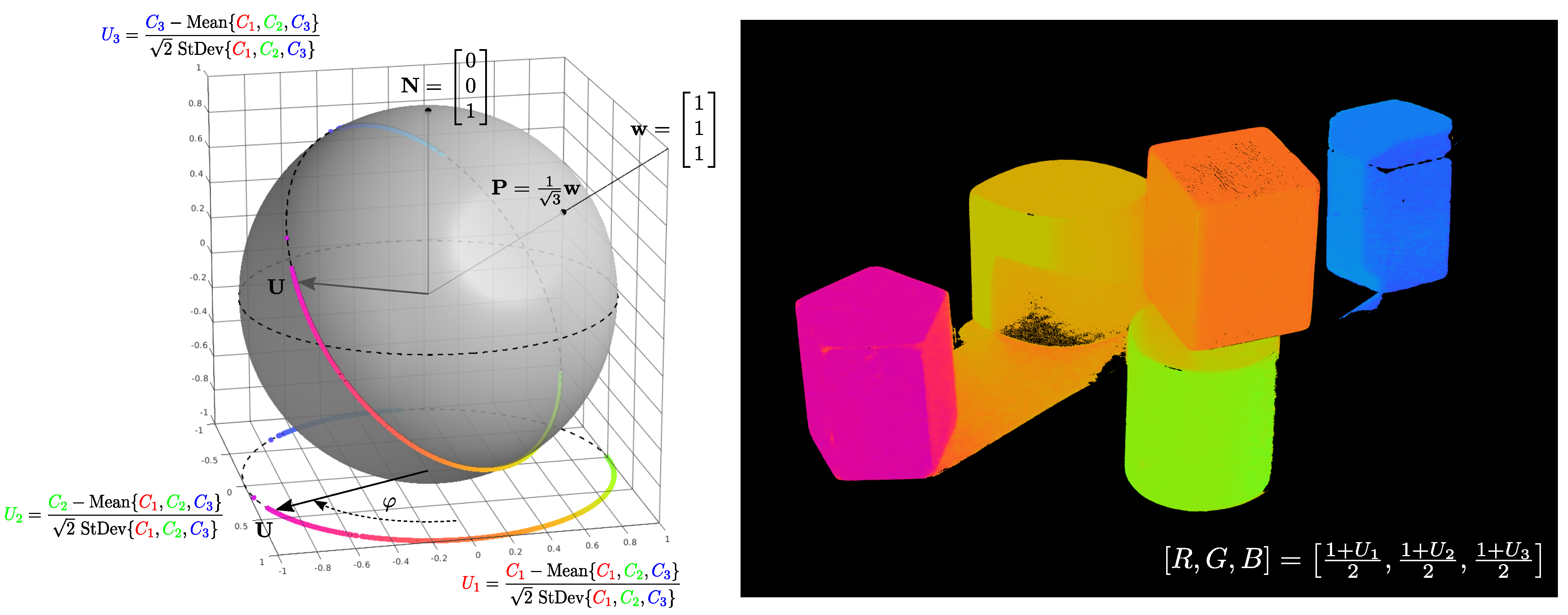
3.2.1. Mathematical Definition

In the resaturation step, we choose to remove the pixel-wise mean of all bands, instead of the minimum. We obtain the vector c with entries:
c i = C i 1 n j = 1 n C j
Then, instead of normalizing with the sum of the resulting entries, we simply normalize this vector with its Euclidean norm, yielding the vector invariant U :
U = c c
The entries of this vector read explicitely:
U i = c i j = 1 n c j 2 = C i 1 n j = 1 n C j j = 1 n C j 2 1 n j = 1 n C j 2 = C i Mean j C j n 1 StDev j C j

3.2.2. Illustration with the RGB Image

Just as we did for the invariant L ( M ) of Montoliu et al. [16], in Figure 5 we show the resulting transformed image and the location of transformed pixel values in the invariant space. It is worth noting that the transformation does not preserve the positivity of entries U i . However, since U has unit norm, it lies in the [ 1 , 1 ] × [ 1 , 1 ] × × [ 1 , 1 ] cube and U i + 1 2 will remain inside the positive-valued unit cube; we use these values to reconstruct the R, G, and B components.
This time, it is the resaturation condition that must be interpreted as a scalar product. Centering the values implies:
j U j = 0 U · w = 0
Again, the invariant lies in a subspace (a plane in R 3 ) orthogonal to the ‘white’ vector w . Moreover, it has unit norm by virtue of the normalization step: as a result, it directy lies on a great circle (‘tilted’ equator). Rotating the white axis onto the last Cartesian axis will again allow us to discard this last coordinate: we are left with a circle that can be described with only two Cartesian coordinates and only one angular coordinate.
This property will extend in any dimension: the multispectral hue U will always belong to a subset homeomorphic to S n 2 the unit ( n 2 ) -sphere embedded in R n 1 , provided that we perform a final rotation that aligns the ‘white’ direction w onto the ‘North Pole’ n = [ 0 , 0 , , 0 , 1 ] T of R n . The general expression of the corresponding rotation matrix is given in Appendix A.

3.2.3. Summary of the Section

In this section, we defined a multispectral hue, which is an extension of the classical RGB hue to a higher number of bands: it allows us to resaturate and normalize the brightness of each pixel, whatever the number of bands. [7]. This multispectral hue denoted U is a direction (unit vector) in a ( n 1 ) dimensional Euclidean space, and it has ( n 2 ) angular degrees of freedom:
  • With n = 3 bands, U is on S 1 the unit circle in the Euclidean plane R 2 : it is closely related to the ‘color wheel’;
  • With n = 4 bands, U is on S 2 the ‘usual’ unit sphere in the Euclidean space R 3 . It has two degrees of freedom, we might call them ‘color latitude’ and ‘color longitude’ as will be seen later;
  • With n > 4 bands, the hypersphere S n 2 cannot be pictured out. However, it is still a smooth Riemannian manifold, and all familiar properties on S 1 and S 2 (geodesic distance, Euler angles, rotation group, etc.) can be extended to any dimension.
We can then use directional statistics to analyze hue distributions in any dimension.

3.3. Mixture Models for the Analysis of Multispectral Hue Distribution

The distribution of multispectral hues in a given image can be rather complicated. For this reason, it may be convenient to model the probability density function of this directional variable as a mixture of simpler distributions. On the color wheel S 1 for the RGB image displayed in Figure 3, we can use the Von Mises distribution as a basic component; its density reads:
f ( φ | μ , κ ) = e κ cos ( φ μ ) 2 π I 0 ( κ )
where φ is the hue angle, μ the mean angle, κ a concentration parameter and I 0 the modified Bessel function of order 0 for normalization. This density can also be written with vectors; noting
U = cos φ sin φ v m = cos μ sin μ
then
f ( U | v m , κ ) = e κ v m · U 2 π I 0 ( κ )
where v m is now the mean (vector) direction.

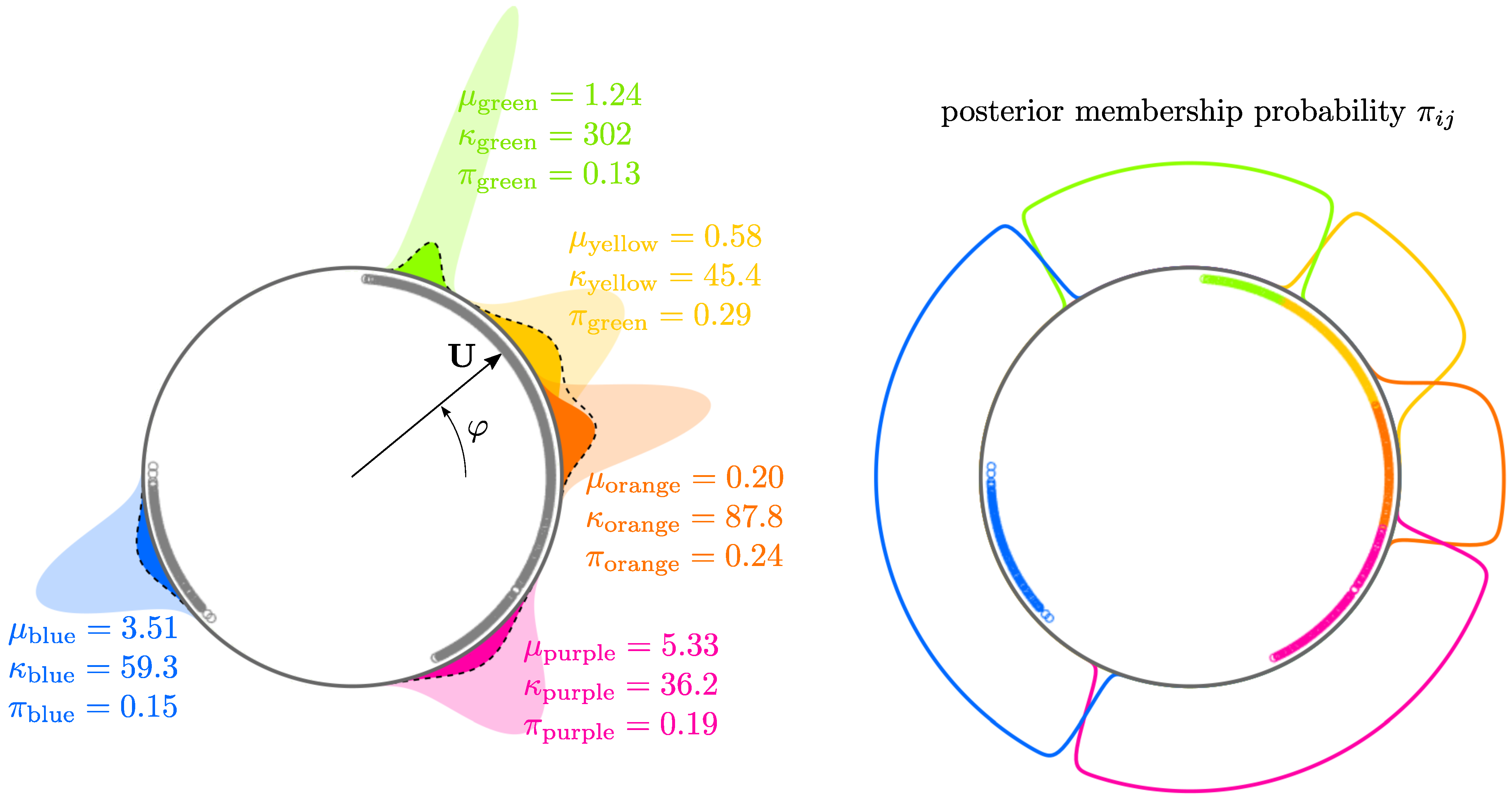
3.3.1. Mixture Density

Having chosen the elementary component, the mixture density is simply a weighted sum of m components:
f ( φ ) = j = 1 m π j f j ( φ | μ j , κ j )
The resulting density still has to sum to unity on the circle, so the weights must sum to 1:
S f ( U ) d S = 0 2 π f ( φ ) d φ = 1 j = 1 m π j = 1
Figure 6 (left) shows the modeled density of hue in our RGB image: we use a five-component model, one for each wooden shape.

3.3.2. Parameter Estimation Using Expectation–Maximization Algorithm

It is necessary to present briefly how the parameters { μ j , κ j , π j } j = 1 m of the mixture density are estimated, because we will use a variant of this procedure for depth estimation. The procedure used is the iterative expectation–maximization (EM) algorithm [18]:
  • E-step (Expectation): at each iteration ( r ) , we start with current parameter estimates μ j ( r ) ; κ j ( r ) ; π j ( r ) j = 1 m and we define updated membership probabilities using Bayes formula:
    π i j ( r + 1 ) = π j ( r ) f j φ i | μ j ( r ) , κ j ( r ) j = 1 m π j ( r ) f j φ i | μ j ( r ) , κ j ( r )
    where π i j ( r + 1 ) is the estimated probability that pixel i with hue angle φ i comes from component j, with j = 1 m π i j ( r + 1 ) = 1 for each pixel;
  • M-step (Maximization): given these membership probabilities, the parameters of each component are re-estimated using a slightly modified maximum likelihood method based on the maximization of:
    j μ j , κ j = i = 1 N pix π i j ( r + 1 ) log f j φ i | μ j , κ j
    We see that the weights in this log-likelihood are the membership probabilities, instead of just 1. j μ j , κ j can be maximized for each component j independently, leading to updated parameters μ j ( r + 1 ) , κ j ( r + 1 ) and
    π j ( r + 1 ) = i = 1 N pix π i j ( r + 1 )

4. Using Multispectral Hue as a Predictor for Depth

In this section, we test our newly-defined multispectral hue as a predictor for depth on a 35-km reach of the Garonne River between Toulouse and Verdun-sur-Garonne (see Figure 7 left). This reach has a rather natural morphology with few embankments past Toulouse, and many wetlands (it is dubbed the “Garonne débordante”, which means “overflowing Garonne” in French). The average channel width is about 150 m and the maximum depth about 5-6 m at low flow. The channel is mainly bedrock, with typical sculpted molassic forms [19] and several major knickpoints with very shallow flow (depth < 1 m).
This site has been widely used in the French remote sensing community to test discharge estimation algorithms using water surface elevation measurements such as the ones that will be produced by the joint NASA and CNES ‘Surface Water and Ocean Topography’ (SWOT) mission [20,21,22]. As our study contributes to these developments, we needed to produce a detailed bathymetric map on this specific reach, and we present the results in this section. As it will be shown further on, the dataset used has some flaws that prevent us from drawing very general conclusions regarding the advantages of the method. A full qualification of the method is needed and will be the object of a future publication using other publicly available datasets [23].

4.1. Dataset

4.1.1. High-Resolution Airborne Imagery

Our study is based on the BD ORTHO® database provided by the IGN (French National Geographic Institute). This nationwide dataset consists of RGB and Infrared Color (IRC) ortho-rectified and radiometrically corrected airborne images [24,25] with a resolution of 0.50 m. For our area of interest, we use images acquired during the period 17–30 July, 2016. This dataset provides us with four coregistered spectral bands, namely near-infrared (NIR), red, green, and blue.

4.1.2. In Situ Depth Measurements

As mentioned in Section 2, the relationship between hue and depth can be determined either physically (using radiative modeling) or empirically, using calibration against in situ data. In this study, we use the latter approach: the relationship is calibrated against in situ bathymetric data collected at 120 cross-sections along the reach (about 1 section every 400 m). These data were collected during surveys in the period 1987–2002: hence, this end-of-20th-century bathymetry may differ substantially from present bathymetry locally, even for a bedrock channel (this point will be discussed at the end of the paper).

4.1.3. LiDAR Data in the Floodplain

In order to better constrain the estimation of river depth, we use LiDAR elevation data available in the floodplain. These data come from the BDORTHO® database also provided by IGN. Even though raster tiles are without gaps, elevation data in the river channel must be ignored: the value at a pixel located in the channel is simply the result of an interpolation between nearby bank pixels. In order to filter out interpolated pixels, the BDORTHO® elevation rasters come with useful ancillary DST (dist) rasters, which indicate the distance of each pixel to the nearest valid LiDAR point (see Figure 8 right).

4.2. Hue Sphere S 2 for n = 4 Bands

According to the approach presented in Section 3, with n = 4 the invariant U does not lie on the circle (1-sphere S 1 ) but on the ( n 2 ) -sphere, i.e., the classical sphere S 2 . In Appendix B, we give the computational detail of the mapping of a 4-band pixel ( C R 4 ) onto the unit sphere U on S 2 . Here is the final mapping of the four ‘monochromatic’ points, in Cartesian coordinates of R 3 :
C NIR = [ 1 , 0 , 0 , 0 ] T U NIR = 1 3 3 [ 5 , 1 , 1 ] T C Red = [ 0 , 1 , 0 , 0 ] T U Red = 1 3 3 [ 1 , 5 , 1 ] T C Green = [ 0 , 0 , 1 , 0 ] T U Green = 1 3 3 [ 1 , 1 , 5 ] T C Blue = [ 0 , 0 , 0 , 1 ] T U Blue = 1 3 3 [ 3 , 3 , 3 ] T
In order to illustrate how the hue (hyper)sphere works, we show in Figure 9 where two patches will map, along with the four ‘monochromatic’ points mentioned above. The first patch (A) is composed of water pixels: as absorption is much stronger in IR than in any of the visible bands, it is no surprise that these pixels will map close to the ‘anti-NIR’ hue, corresponding to the multispectral hue of a pixel with digital counts [ 0 , 1 , 1 , 1 ] T . Conversely, a patch of vegetation (B) will map close to the pure NIR hue, as absorption is not the same in all visible bands but still much stronger than in the NIR.

4.3. Masks

In order to reduce the extent of the area investigated and to narrow the spread of hue distributions, several boolean masks are applied on the raw images in order to retain only river pixels, as illustrated in Figure 10:
  • Riparian vegetation as well as floating algae are masked using the classical Normalized Difference Vegetation Index (NDVI) [26], which indicates high chlorophyll content. In practice, the rather low threshold selected (NDVI > −0.3) excludes more than just vegetation pixels: all surfaces with any non-negligible reflectance in the IR will be masked;
  • Very dark areas are thoroughly removed: they mainly consist of water pixels in the shadow of riparian vegetation; as these pixels are difficult to characterize spectrally (light has traveled through both leaves and water), the criterion used is simply the mean of the four bands;
  • A filter is designed to remove whitewater/white wakes in riffle areas: as these pixels appear in light gray in the visible bands (almost hueless in RGB) but with substantial absorption in the IR (typical digital counts are [0.2 0.6 0.6 0.6]), they are removed on the basis of their low saturation and high brightness in the RGB space along with a threshold in the NIR ( C NIR < 0.3 ). Note that they have nothing to do with specular reflections: the surface of water appears white there for any viewing angle, because of the scattering from the bubbles/air pockets, not from surface reflection;
  • A mask for man-made features crossing the river, such as bridges or power lines as well as their casted shadows, is built manually (some of these pixels are already masked by the previous filters, but not all).
Once all these masks are combined, a final topological erosion of the resulting mask is performed.

4.4. Hue–Depth Visual Correlation on S 2

We now focus on river pixels with a valid multispectral hue. We can first look at the projection onto the sphere of all pixels located at depth measurement points. What we see first in Figure 11 is that they are located close to the anti-NIR hue, as already mentioned above. However, if we plot them with measured depth as color, we see that ‘deep’ pixels tend to concentrate close to a single pole of the sphere. This result is perfectly consistent with Philpot’s Equation (2): as depth increases, the weight of bed reflectance R b in the mixture reflectance vanishes to zero and the digital counts of river pixels, which are basically reflectances, should tend to the limit vector
C c , R c , ( λ NIR ) R c , ( λ Red ) R c , ( λ Green ) R c , ( λ Blue )
The hue associated with C c , is thus some point U c , on S 2 , that we can roughly locate visually. Here, ‘infinitely’ deep means about 5 to 6 m deep.

4.5. Mixture Models on S 2 and Higher Dimension, and Depth Predictor

Our last step is to find a quantitative predictor for depth. The two principles are the following:
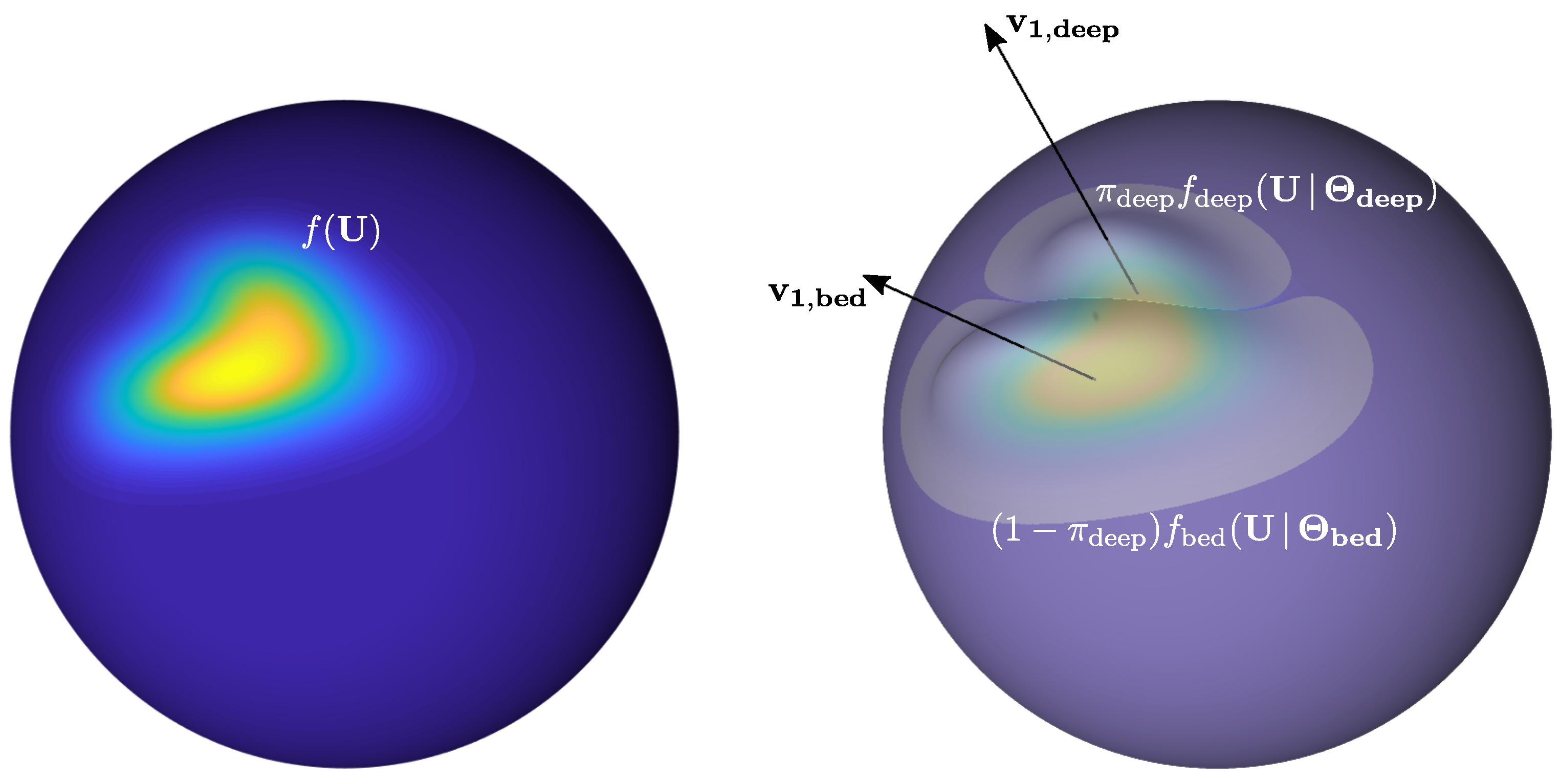
  • We assume that the probability density function of multispectral hue in river pixels can be modeled by a two-component mixture density: the first component will represent the statistical distribution of substrate hue, while the second component will represent the statistical distribution of ‘deep water’ hue;
  • We will estimate the parameters of the two components so that the membership probability to ‘deep’ component correlates with depth: the probability π i , deep that pixel i with hue U i comes from the ‘deep’ component will be the predictor for depth h i at pixel i.
The elementary component used on the unit circle S 1 in Section 3 is the Von Mises distribution (‘circular normal distribution’). On the unit sphere S 2 and higher dimension, we need an extension of this distribution, similar to a multivariate normal distribution wrapped on the (hyper)sphere. Such an extension is the Fisher–Bingham–Kent (FBK) distribution [27]; for the sake of clarity, basic details about this family of distributions are provided in Appendix C. For U S n 2 , the density reads:
f U | v j , κ , β = 1 C ( κ , β ) exp κ v 1 · U + j = 2 n 1 β j ( v j · U ) 2
The ( n 1 ) vectors v j for 1 j ( n 1 ) form an orthonormal basis in which the first vector v 1 is the mean direction of the distribution, as f is maximum when v 1 · U = 1 . The normalization constant C ( κ , β ) does not have a closed form, but it can be evaluated numerically [28,29]. The number of degrees of freedom increases almost quadratically with the number of bands ( 1 2 n 2 ).
Figure 12 illustrates the decomposition of a given density on S 2 into two FBK components. In our case, the two components will be the distributions f bed of bed substrate hue and f deep of deep water hue, respectively; for the sake of concision, we denote Θ bed and Θ deep the parameter set describing each component, so that the mixture density reads:
f ( U ) = π deep f deep U | Θ deep + ( 1 π deep ) f bed U | Θ bed

4.6. Modified EM Algorithm for Depth Estimation

The goal of the calibration process is, in the end, to be able to correlate depth h i at an ‘unmeasured’ pixel i having multispectral hue U i , with the posterior membership probability to the deep component:
π i , deep = π deep f deep U i | Θ deep π deep f deep U i | Θ deep + 1 π deep f bed U i | Θ bed
Recall that the ‘posterior’ term means ‘after we get the additional information of pixel hue’. In contrast, π deep is the ‘prior’, general probability that a randomly choosen pixel comes from the deep component (it is a constant, corresponding to the weight of the deep component in the mixture distribution): once we obtain the multispectral hue U i for a particular pixel i, we can update the prior membership probability using Bayes formula to obtain the individual posterior membership probability π i , deep .
In order for this posterior probability to be correlated with depth, we use a slightly modified version of the expectation–maximization algorithm presented in Section 3, where we first estimated membership probabilities for each pixel (expectation E-step) and then updated the parameters of each component independently using the updated membership probabilities (maximization M-step). Here, we will add an intermediate regression (R-step) between these two steps: instead of feeding the maximization algorithm directly with the membership probabilities π i , deep ( r + 1 ) for each pixel, we will regress the π i , deep ( r + 1 ) against measured depth h i and feed the maximization algorithm with regressed membership probabilities π ^ i , deep ( r + 1 ) ( h i ) . Here is the workflow performed at each iteration:
  • E-step (Expectation): given current parameter estimates π deep ( r ) ; Θ deep ( r ) ; Θ bed ( r ) of the mixture at iteration ( r ) , compute the updated probability that pixel i with multispectral hue U i comes from a deep component:
    π i , deep ( r + 1 ) = π deep ( r ) f deep U i | Θ deep ( r ) π deep ( r ) f deep U i | Θ deep ( r ) + 1 π deep ( r ) f bed U i | Θ bed ( r )
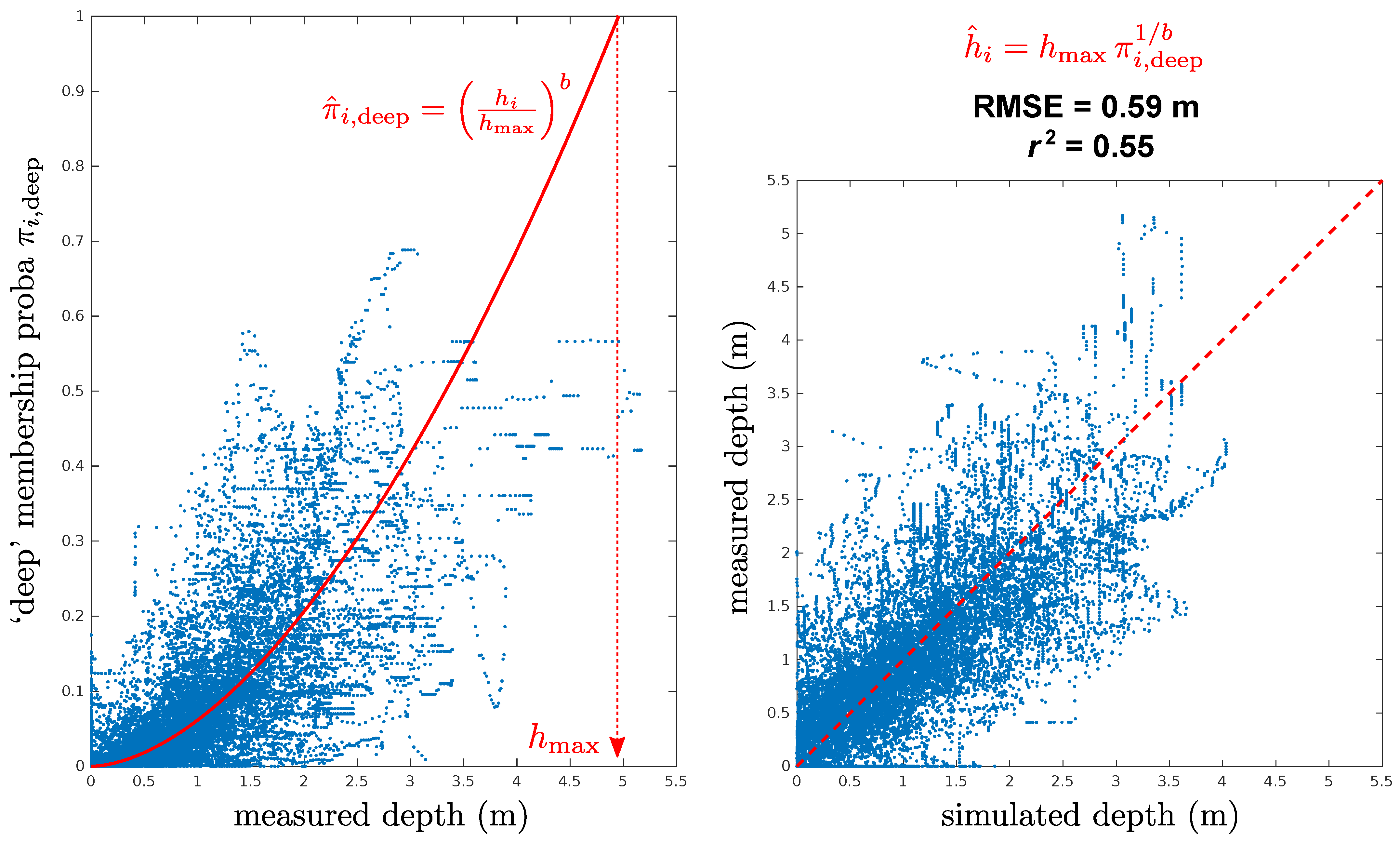
  • R-step (Regression): regress deep membership probability as a power law function of measured depth so that
    π ^ i , deep ( r + 1 ) = a ( r + 1 ) h i b ( r + 1 )
  • M-step (Maximization): independently maximize the log-likelihood for each component
    deep Θ deep = i = 1 N depth π ^ i , deep ( r + 1 ) log f deep U i | Θ deep updated Θ deep ( r + 1 ) bed Θ bed = i = 1 N depth 1 π ^ i , deep ( r + 1 ) log f bed U i | Θ bed updated Θ bed ( r + 1 )
    Finally, we update the prior membership probability π deep (weight of the deep component in the mixture), which is the mathematical expectation of individual (posterior) membership probabilities:
    π deep ( r + 1 ) = 1 N depth i = 1 N depth π ^ i , deep ( r + 1 )
where N depth is the total number of in situ depth measurement points. Then we iterate back at E-step and so on until convergence is reached.

5. Results

5.1. Error Statistics

The modified expectation–maximization algorithm has several outputs after convergence: the final parameters π deep ; Θ deep ; Θ bed of the mixture, but also the regression parameters ( a , b ) such that for each pixel i
π ^ i , deep = a h i b
This output curve is shown in Figure 13, left panel. Taking h max = a 1 / b , this relation can be reversed in order to express depth as a function of (known) posterior membership probability:
h ^ i = h max π i , deep 1 / b
Since π i , deep ranges between 0 and 1, estimated depth cannot exceed the ‘saturation’ value h max , which is found to be about 4.9 m. In other words, when hue is close to the maximum of the density of the ‘deep’ component, all we can say is that depth is at least h max , but could be much larger. This is a reasonable behavior: the model will never extrapolate to unbounded values. Figure 13, right panel, shows the resulting scatter plot for estimated vs. measured depth: the RMSE is about 0.59 m and the determination coefficient is r 2 = 0.55 .
In Figure 14, we plot the correlation between measured depth and the log of all spectral ratios that can be defined with four bands. Obviously, no single pair of bands exhibits a correlation stronger than the one identified on the hue hypersphere. Most noticeably, none of the spectral ratios is able to identify large depths unambiguously.
A simple benchmark is provided by a Multiple Linear (ML) regression using all independent log-ratios (i.e., ratios between pairs of adjacent bands). It is a specific type of MODPA analysis [15] and the resulting optimal combination of predictors reads:
h ML = 2.60 log Red NIR + 11.48 log Green Red 7.31 log Blue Green 7.39
The result is shown in Figure 15: the model yields an RMSE of 0.58 m, roughly similar to our procedure. However, the correlation is substantially lower: due to the least-square nature of the model, the variance of estimated depth is lower than the variance of measured depth and the model is not able to yield depths larger than 2.5 m. In contrast, the mixture model on the hypersphere yields depths as large as 4 m.

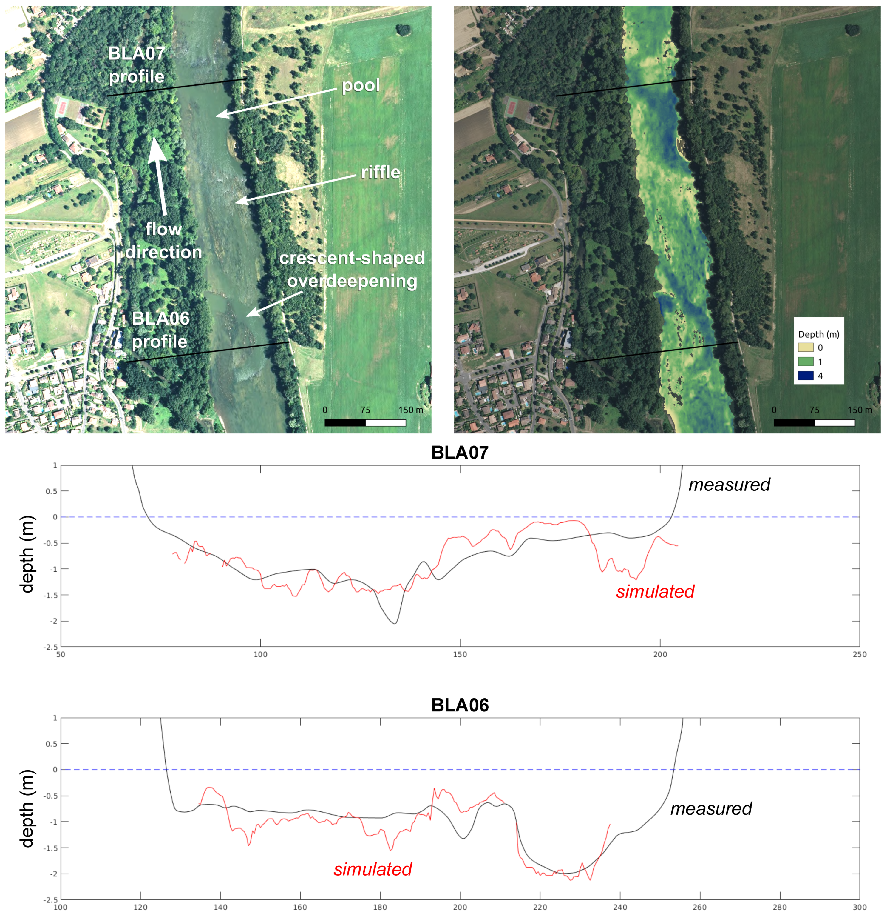
5.2. Focus on Some Cross-Sections

In Figure 16, we show measured and simulated depth at two representative cross-sections. This illustrates how the method is able to identify localized bed features and high-frequency variations in bathymetry, which are typical of the bedrock channel of the Garonne Toulousaine [19].

6. Discussion

6.1. Sources of Error

6.1.1. Radiometric Inhomogeneity

The BDORTHO® images used in this study form a nationwide dataset covering all 101 French departments. In practice, these images are radiometrically equalized in order to provide a seamless mosaic at the scale of each department [24,25]. There remain some variations in radiometric aspects inside the mosaic, and especially at the border between two departments. As the investigated reach spans two departments, namely Haute-Garonne (31) and Tarn-et-Garonne (82), the dataset is clearly not radiometrically homogeneous, and this increases the variability in both substrate and deep water hue. This additional variability reduces the precision of the hue—depth relation, but since the method is designed to deal with a dispersion in the distribution of both components through parameter sets Θ bed and Θ deep of the Fisher–Bingham–Kent distributions, the radiometric inhomogeneity can be statistically treated together with the natural variations. The key parameter acting as a quantification of non-uniformity is the concentration parameter κ bed of the bed hue distribution. This is an important advantage of the method over log-ratio methods, which rely on the assumption that reflectance ratios R b ( x , λ i ) R b ( x , λ j ) are rather uniform spatially (see Section 2).

6.1.2. Age and Planar Precision of In Situ Data

As mentioned in Section 4.1.2, the bathymetric data used in this study were collected during surveys in the period 1987–2002. This end-of-twentieth-century bathymetry may differ substantially from present bathymetry locally, even for a bedrock channel. Moreover, a precise positioning of profile with GPS was not always available: errors up to several meters on the transverse position of cross-section points were obvious for a few of them, and likely for many. Profiles were manually repositioned where it was possible, but the remaining uncertainty is an important source of error.

6.1.3. Water Surface Elevation

The airborne images were taken at low flow during the month of July, 2016. However, we do not have a corresponding water surface profile of the reach for the same period; as in situ data consists of absolute bed elevation z b (in meters a.s.l) and not depth, we needed an estimated map of water surface elevation z w s at low flow, which we derived from a mean of two estimates:
  • The first estimate was simply given by the lowest valid elevation at each cross-section in the LiDAR DEM of the floodplain (which also covers the channel through interpolation between the banks). Indeed, the LiDAR survey was conducted during the 2012 low flow period, in hydraulic conditions that we assumed roughly similar to those of the 2016 images;
  • The second estimate is the elevation that yields the same width as the one observed in the 2016 images (as defined by the NDWI mask), for each surveyed profile. We then interpolate linearly between the surveyed cross-sections.
We then corrected the values so that our estimated low flow surface elevation profile has strictly monotonically decreasing values. Even if the estimated water surface profile seems reasonable, the uncertainty in water surface elevation, and hence in field estimate of water depth h = z w s z b , may be several tens of centimeters locally. As large depths drive the parameter estimation, it does not hinder the possibility to identify a robust hue–depth relation, though.

6.2. Perspectives

This work is a proof-of-concept that large-scale identification of river bathymetry is possible using publicly available nationwide datasets. The bathymetric map of the Garonne River produced in this study will be used as an input for reach-scale hydraulic modeling and the analysis of reach-scale hydraulic geometry relationships following [2], with a spatial resolution that could never have been achieved on the sole basis of existing in situ data. However, the shortcomings of the Garonne dataset, listed in Section 6.1, make it necessary to continue the work using higher-quality data.

Author Contributions

Conceptualization, N.L.M. and M.M.; software, N.L.M.; data curation and validation, N.L.M. and M.M.; supervision and project administration, N.L.M. All authors have read and agreed to the published version of the manuscript.

Funding

This research received partial external funding through the Ph.D. grant of Mounir Mahdade (SU C18/1749-S18LRAP039/CNES 510004634).

Data Availability Statement

The tiles of the BDORTHO® dataset used in this study are publicly available from IGN Open-Access portal (accessed 14 December 2020): https://geoservices.ign.fr/documentation/diffusion/telechargement-donnees-libres.html.

Acknowledgments

We thank the Direction Régionale de l’Environnement, de l’Aménagement et du Logement (DREAL) Occitanie and the Syndicat Mixte d’Études et d’Aménagement de la Garonne (SMEAG), as well as Hélène Roux and André Paquier, for providing the cross-section data. We thank Katell for providing the experimental material of Section 3.

Conflicts of Interest

The authors declare no conflict of interest.

Appendix A. General Expression of the Rotation Matrix Needed for Computing the Multispectral Hue in Any Dimension

Let w and n be two unit vectors of vectors of R n (i.e., two points of S n 1 ). The n-dimensional rotation matrix sending w on n can be obtained as follows [30]. Noting
α = arccos ( w · n ) = arccos w T n
q = w n cos α w n cos α
A = n q q n
where n q = n q T is the outer (dyadic) product, the desired rotation matrix is
M = I + ( sin α ) A + ( cos α ) 1 n n + q q
The rotation matrix allowing the transition from S n 1 to S n 2 in the last step of hue computations is the one sending the ‘unit white vector’ w = 1 n [ 1 , 1 , , 1 , 1 ] T of R n to the ‘North Pole’ n = [ 0 , 0 , , 0 , 1 ] T of R n .
In R 4 , this matrix reads:
M = 1 6 5 1 1 3 1 5 1 3 1 1 5 3 3 3 3 3 with M 1 = M T M T M = I , and det ( M ) = + 1

Appendix B. Computational Example of the Mapping from R 4 to S 2 with Four Bands

In this Appendix, we detail the computations mapping a ‘pure green’ pixel C Green = [ 0 , 0 , 1 , 0 ] T onto the unit hue sphere S 2 .
  • We first remove the mean of all bands to each band in order to obtain the vector c , and then we normalize it:
    c Green = 1 / 4 1 / 4 + 3 / 4 1 / 4 c Green c Green = 2 3 1 / 4 1 / 4 + 3 / 4 1 / 4 = 1 2 3 1 1 + 3 1
  • The latter vector is already on a two-sphere, but this sphere is embedded in a three-dimensional subspace of R 4 whose axes do not coincide with a triplet of axes of the initial basis (this three-dimensional subspace is orthogonal to the unit ‘white’ vector w = 1 2 [ 1 , 1 , 1 , 1 ] T ). In order to drop one Cartesian coordinate (e.g., the last one), we rotate w to the ’North Pole’ n = [ 0 , 0 , 0 , 1 ] T of R 4 , with the 4D rotation matrix M such that:
    M w = M 1 / 2 1 / 2 1 / 2 1 / 2 = 0 0 0 1 = n
    Performing this final rotation and discarding the last, the zero coordinate yields:
    U Green = M c Green c Green = 1 12 3 4 4 20 0 1 3 3 1 1 5 R 3
  • Here we express U in Cartesian coordinates of R n 1 , but we can check that it is indeed in S n 2 :
    U Green = 1 3 3 ( 1 ) 2 + ( 1 ) 2 + 5 2 = 1 3 3 27 = 1
It is often easier to manipulate the invariant in Cartesian coordinates of R n 1 , instead of ( n 2 ) Euler angles: one reason is that computations on a hypersphere involve many scalar products which are straightforwardly evaluated in Cartesian coordinates. However, we must always recall that the invariant has only ( n 2 ) degrees of freedom.

Appendix C. Overview of the Fisher–Bingham–Kent (FBK) Distribution

In this appendix, we provide a quick overview of the properties of the Fisher–Bingham–Kent distribution for a random vector x on the ( p 1 ) -sphere S p 1 embedded in R p . We remind that in the paper, p = n 1 where n is the number of bands. The probability density function reads:
f ( x ; v j , κ , β ) = 1 C ( κ , β ) exp κ v 1 · x + j = 2 p β j ( v j · x ) 2
j = 2 p β j = 0 0 < β j κ 2 v i · v j = v i T v j = δ i j vectors form an orthonormal basis
κ > 0 is a concentration parameter controlling the dispersion around the mean direction v 1 : indeed, the term ( κ v 1 · x ) is maximum when the scalar product is 1, for x = v 1 , and minimum when the scalar product is 1 , in x = v 1 (antipode of v 1 ). Constants β j and vectors v j j = 2 p determine the asymetry of the distribution in the ( p 1 ) directions orthogonal to v 1 .
The Fisher–Bingham–Kent distribution thus has N = ( p 1 ) ( p + 2 ) 2 degrees of freedom, distributed in:
  • Degrees of freedom corresponding to the minimum number of rotations (aside from degenerated cases) allowing the change-of-basis from the canonical basis of R p to the orthonormal basis defined by the v j ; there are as many such rotations as independent rotation planes in R p , that is, the number of combinations of two orthogonal directions chosen from among p:
    p 2 = C p 2 = p ! ( p 2 ) ! 2 ! = 1 2 p ( p 1 )
  • p degrees of freedom corresponding to the concentration parameter κ and the ( p 1 ) asymetry parameters β j , 2 j p ,
  • 1 degree of freedom removed due to the condition on the β j
    j = 2 p β j = 0
Table A1 below summarizes the number of parameters of the FBK distribution depending on the number of bands (n) or dimension of the corresponding Euclidean space p = n 1 ( U S n 2 R n 1 ).
Table A1. Number N of degrees of freedom for the Fisher–Bingham–Kent distribution as a function of the dimension p of the initial space.
n Number of Bands p = n 1 Euclidean SpaceHypersphere N = ( p 1 ) ( p + 2 ) 2 Remark
32 R 2 S 1 (circle)2Von Mises distribution
43 R 3 S 2 (sphere)5classical Fisher–Bingham “FB5”
54 R 4 S 3 9
109 R 9 S 8 44
5049 R 49 S 48 1224
10099 R 99 S 98 4949

References

  1. Wyrick, J.; Pasternack, G. Geospatial organization of fluvial landforms in a gravel–cobble river: Beyond the riffle–pool couplet. Geomorphology 2014, 213, 48–65. [Google Scholar] [CrossRef] [Green Version]
  2. Mahdade, M.; Le Moine, N.; Moussa, R.; Navratil, O.; Ribstein, P. Automatic identification of alternating morphological units in river channels using wavelet analysis and ridge extraction. Hydrol. Earth Syst. Sci. 2020, 24, 3513–3537. [Google Scholar] [CrossRef]
  3. Kinzel, P.J.; Wright, C.W.; Nelson, J.M.; Burman, A.R. Evaluation of an Experimental LiDAR for Surveying a Shallow, Braided, Sand-Bedded River. J. Hydraul. Eng. 2007, 133, 838–842. [Google Scholar] [CrossRef] [Green Version]
  4. Hilldale, R.C.; Raff, D. Assessing the ability of airborne LiDAR to map river bathymetry. Earth Surf. Process. Landforms 2008, 33, 773–783. [Google Scholar] [CrossRef]
  5. Nakao, L.; Krueger, C.; Bleninger, T. Benchmarking for using an acoustic Doppler current profiler for bathymetric survey. Environ. Monit. Assess. 2021, 193, 356. [Google Scholar] [CrossRef] [PubMed]
  6. Lyzenga, D.R. Passive remote sensing techniques for mapping water depth and bottom features. Appl. Opt. 1978, 17, 379–383. [Google Scholar] [CrossRef] [PubMed]
  7. Marcus, W.A.; Fonstad, M.A. Optical remote mapping of rivers at sub-meter resolutions and watershed extents. Earth Surf. Process. Landforms 2008, 33, 4–24. [Google Scholar] [CrossRef]
  8. Legleiter, C.J.; Roberts, D.A.; Lawrence, R.L. Spectrally based remote sensing of river bathymetry. Earth Surf. Process. Landforms 2009, 34, 1039–1059. [Google Scholar] [CrossRef]
  9. Campbell, J.B. Introduction to Remote Sensing, 2nd ed.; The Guilford Press: New York, NY, USA, 1996. [Google Scholar]
  10. Philpot, W.D. Bathymetric mapping with passive multispectral imagery. Appl. Opt. 1989, 28, 1569–1578. [Google Scholar] [CrossRef]
  11. Shah, A.; Deshmukh, B.; Sinha, L. A review of approaches for water depth estimation with multispectral data. World Water Policy 2020, 6, 152–167. [Google Scholar] [CrossRef]
  12. König, M.; Oppelt, N. A linear model to derive melt pond depth from hyperspectral data. Cryosph. Discuss 2019, 2019, 1–17. [Google Scholar]
  13. König, M.; Birnbaum, G.; Oppelt, N. Mapping the Bathymetry of Melt Ponds on Arctic Sea Ice Using Hyperspectral Imagery. Remote Sens. 2020, 12, 2623. [Google Scholar] [CrossRef]
  14. Doxani, G.; Papadopoulou, M.; Lafazani, P.; Pikridas, C.; Tsakiri-Strati, M. Shallow-water bathymetry over variable bottom types using multispectral Worldview-2 image. Int. Arch. Photogramm. Remote Sens. Spat. Inf. Sci. 2012, 39, 159–164. [Google Scholar] [CrossRef] [Green Version]
  15. Niroumand-Jadidi, M.; Vitti, A.; Lyzenga, D.R. Multiple Optimal Depth Predictors Analysis (MODPA) for river bathymetry: Findings from spectroradiometry, simulations, and satellite imagery. Remote Sens. Environ. 2018, 218, 132–147. [Google Scholar] [CrossRef]
  16. Montoliu, R.; Pla, F.; Klaren, A.C. Illumination Intensity, Object Geometry and Highlights Invariance in Multispectral Imaging. In Proceedings of the Second Iberian Conference on Pattern Recognition and Image Analysis—Volume Part I; IbPRIA’05. Springer: Berlin/Heidelberg, Germany, 2005; pp. 36–43. [Google Scholar] [CrossRef] [Green Version]
  17. Kay, S.; Hedley, J.D.; Lavender, S. Sun Glint Correction of High and Low Spatial Resolution Images of Aquatic Scenes: A Review of Methods for Visible and Near-Infrared Wavelengths. Remote Sens. 2009, 1, 697–730. [Google Scholar] [CrossRef] [Green Version]
  18. Dempster, A.P.; Laird, N.M.; Rubin, D.B. Maximum Likelihood from Incomplete Data via the EM Algorithm. J. R. Stat. Soc. Ser. B Methodol. 1977, 39, 1–38. [Google Scholar]
  19. Jantzi, H.; Carozza, J.M.; Probst, J.L. Les formes d’érosion en lit mineur rocheux: Typologie, distribution spatiale et implications sur la dynamique du lit. Exemple à partir des seuils rocheux molassiques de la moyenne Garonne toulousaine (Sud-Ouest, France). Géomorphologie 2020, 26, 79–96. [Google Scholar] [CrossRef]
  20. Garambois, P.A.; Biancamaria, S.; Monnier, J.; Roux, H.; Dartus, D. Variationnal data assimilation of AirSWOT and SWOT data into the 2D shallow water model Dassflow, method and test case on the Garonne river (France). In Proceedings of the 20 Years of Progress in Radar Altimetry, Venice, Italy, 24–29 September 2012. [Google Scholar]
  21. Oubanas, H.; Gejadze, I.; Malaterre, P.O.; Mercier, F. River discharge estimation from synthetic SWOT-type observations using variational data assimilation and the full Saint-Venant hydraulic model. J. Hydrol. 2018, 559, 638–647. [Google Scholar] [CrossRef]
  22. Goutal, N.; Goeury, C.; Ata, R.; Ricci, S.; Mocayd, N.E.; Rochoux, M.; Oubanas, H.; Gejadze, I.; Malaterre, P.O. Uncertainty Quantification for River Flow Simulation Applied to a Real Test Case: The Garonne Valley. In Advances in Hydroinformatics; Gourbesville, P., Cunge, J., Caignaert, G., Eds.; Springer: Singapore, 2018; pp. 169–187. [Google Scholar]
  23. Legleiter, C.; Overstreet, B. Hyperspectral image data and field measurements used for bathymetric mapping of the Snake River in Grand Teton National Park, WY. U.S. Geological Survey Data Release, 2018 (accessed 2021-11-02). [CrossRef]
  24. Institut Géographique National. BD ORTHO® Version 2.0/ORTHO HR® Version 1.0: Descriptif de Contenu, May 2013, Updated July 2018. Available online: https://geoservices.ign.fr/ressources_documentaires/Espace_documentaire/ORTHO_IMAGES/BDORTHO_ORTHOHR/DC_BDORTHO_2-0_ORTHOHR_1-0.pdf (accessed on 14 December 2020).
  25. Chandelier, L.; Martinoty, G. Radiometric aerial triangulation for the equalization of digital aerial images and orthoimages. Photogramm. Eng. Remote Sens 2009, 75, 193–200. [Google Scholar] [CrossRef]
  26. Kriegler, F.; Malila, W.; Nalepka, R.; Richardson, W. Preprocessing transformations and their effects on multispectral recognition. Remote Sens. Environ. 1969, 6, 97. [Google Scholar]
  27. Kent, J.T. The Fisher-Bingham Distribution on the Sphere. J. R. Stat. Soc. Ser. B Methodol. 1982, 44, 71–80. [Google Scholar] [CrossRef]
  28. Kume, A.; Wood, A.T.A. Saddlepoint Approximations for the Bingham and Fisher-Bingham Normalising Constants. Biometrika 2005, 92, 465–476. [Google Scholar] [CrossRef] [Green Version]
  29. Kume, A.; Preston, S.P.; Wood, A.T.A. Saddlepoint approximations for the normalizing constant of Fisher-Bingham distributions on products of spheres and Stiefel manifolds. Biometrika 2013, 100, 971–984. [Google Scholar] [CrossRef]
  30. Amaral, G.J.A.; Dryden, I.L.; Wood, A.T.A. Pivotal Bootstrap Methods for k-Sample Problems in Directional Statistics and Shape Analysis. J. Am. Stat. Assoc. 2007, 102, 695–707. [Google Scholar] [CrossRef]
Figure 1. Decomposition of total measured radiance over water (adapted from Campbell, 1996 [9]). E is the downwelling solar irradiance (W·m−2), L b , L c , L s and L p are the bed, water column, surface and path radiances, respectively (W·m−2·sr−1).
Remotesensing 13 04435 g001
Figure 2. Screenshot of the color wheel tool in QGIS. The hue or ‘pure color’ is selected along the circle with a single angular degree of freedom (DoF). The two other operations that can be performed are (1) desaturation or (2) decrease in brightness/value.
Remotesensing 13 04435 g002
Figure 3. Katell’s wooden toys under natural sunlight. Note the specular reflection on the front edge of the orange cube, for example, which appears almost white.
Remotesensing 13 04435 g003
Figure 4. Spectral invariant proposed by Montoliu et al., computed on the image of Figure 3. (Left panel): location of transformed pixel values in the RGB unit cube, invariant L ( M ) is constrained in a plane orthogonal to the white vector w = [ 1 , 1 , 1 ] T . (Right panel): transformed RGB image. Note how light reflected from the yellow oval toy produces a yellow hue on the white floor and also alters the hue on the rightmost side of the purple pentagon toy.
Remotesensing 13 04435 g004
Figure 5. Illustration of multispectral hue U computed on the RGB image of Figure 3. (Left panel): location of transformed pixel values on a great circle in a plane orthogonal to white vector w = [ 1 , 1 , 1 ] T . (Right panel): transformed RGB image.
Remotesensing 13 04435 g005
Figure 6. (Left panel) Hue distribution on the ‘wooden toys’ image (the density is the black dashed line), and its modeling with a mixture of 5 Von Mises distributions. We can check that π orange + π yellow + π green + π blue + π purple = 1 . (Right panel) shows the posterior membership probability π i j (given by Bayes formula) that pixel i comes from component j.
Remotesensing 13 04435 g006
Figure 7. Location of the reach of the Garonne river investigated in this study. (a) Location of the reach in the whole Garonne catchment, between Toulouse and Verdun-sur-Garonne; (b) in situ cross-section data used for calibration.
Remotesensing 13 04435 g007
Figure 8. Sample of the IGN BDORTHO® database covering the floodplain. (a) Elevation raster at 1-meter planar resolution; (b) DST raster indicating the distance to the nearest valid LiDAR point for each pixel.
Remotesensing 13 04435 g008
Figure 9. Representation of multispectral hue on the sphere S 2 for two terrain patches: a patch of water pixels (A) and a patch of vegetation pixels (B). Due to the low absorption in the visible bands and high absorption in the IR for water, and the opposite behavior for chlorophyll, the two patches map at the antipode of each other (close to the anti-NIR hue for water, and close to pure NIR hue for vegetation). The image displayed on the right is a NIR-R-G composite.
Remotesensing 13 04435 g009
Figure 10. Illustration of the four masks applied to multispectral images in order to retain only river pixels. The image displayed is a NIR-R-G composite.
Remotesensing 13 04435 g010
Figure 11. Representation of multispectral hue on S 2 for the pixels located at depth measurement points. As depth increases, hue tends to concentrate near a single pole corresponding to the hue of a very deep water column, denoted U c , .
Remotesensing 13 04435 g011
Figure 12. The probability density function f ( U ) of a hue distribution on the sphere (left) can be modeled with a mixture of two or more Fisher–Bingham–Kent distributions (right). For the distribution of hue over river pixels, we used two components denoted f bed and f deep with respective parameters sets Θ bed and Θ deep : v 1 , bed and v 1 , deep to denote the mean direction of each component.
Remotesensing 13 04435 g012
Figure 13. (Left panel): ‘depth’ vs. ‘deep membership probability’ regression as outputted by the modified expectation–maximization. This relation is of course meant to be used in the reverse direction in predictive mode (right panel): given the posterior membership probability π i , deep computed at pixel i with multispectral hue U i , we can estimate depth h i at this pixel.
Remotesensing 13 04435 g013
Figure 14. Correlation between measured depth and the log of the six different spectral ratios that can be defined with four-band imagery.
Remotesensing 13 04435 g014
Figure 15. Result of a Multiple Linear (ML) regression against all three independent log-ratios. Negative predicted values have been set to zero before the computation of RMSE and r 2 .
Remotesensing 13 04435 g015
Figure 16. Comparison between measured and simulated depth along two surveyed cross-sections. The method is able to capture high-frequency variations in water depth: a typical example is the crescent-shaped feature visible at the bottom of the image, which is intersected by profile BLA06.
Remotesensing 13 04435 g016
Publisher’s Note: MDPI stays neutral with regard to jurisdictional claims in published maps and institutional affiliations.

