Abstract
While there are recent researches on hypersonic vehicle-borne multichannel synthetic aperture radar in ground moving target indication (HSV-MC-SAR/GMTI), this article, which specifically explores a robust GMTI scheme for the highly squinted HSV-MC-SAR in dive mode, is novel. First, an improved equivalent range model (IERM) for stationary targets and GMTs is explored, which enjoys a concise expression and therefore offers the potential to simplify the GMTI process. Then, based on the proposed model, a robust GMTI scheme is derived in detail, paying particular attention to Doppler ambiguity arising from the high-speed and high-resolution wide-swath. Furthermore, it retrieves the accurate two-dimensional speeds of GMTs and realizes the satisfactory performance of clutter rejection and GMT imaging, generating the matched beamforming and enhancing the GMT energy. Finally, it applies the inverse projection to revise the geometry shift induced by the vertical speed. Simulation examples are used to verify the proposed GMTI scheme.
1. Introduction
Flight-borne synthetic aperture radars (SAR) provide tremendous potentials to generate microwave imageries of ground moving targets (GMT) [1] and stationary targets. However, due to the flight characteristics of the platforms, traditional SAR processing exhibits some limitations [2]. To be specific, an air-borne SAR possesses a small detection range, as it flies at a low altitude and a low velocity. Likewise, a space-borne SAR [3], due to the high-altitude and static orbit, has a fixed observed area and high requirements of transmitted power [4,5]. On the other hand, hypersonic vehicle-borne SAR (HSV-SAR), which operates at the altitude of 20 to 100 km and speeds in excess of 1700 m/s, could not be processed using traditional SAR algorithms [6,7]. Fortunately, its processing is also not overwhelming since its skipping orbit can be simplified to a dive orbit, as five-sixths of the entire skipping orbit has no acceleration [8,9].
The GMT indication (GMTI) plays an important role in both civilian and military applications [10,11,12], especially for the vehicle detection. There are recent researches on HSV-SAR/GMT indication (GMTI) in the literature. For side-looking HSV-SAR, refs. [6,7] reject the stationary clutters and recover the GMT imageries, and ref. [8] investigates a SAR/GMTI with a dive orbit. Finally, the stationary target [13] and GMT [14,15] imaging of HSV-SAR are studied, in combination with squint-looking and a. horizontal orbit. On the other hand, there is no GMTI scheme for the HSV-borne multichannel SAR (HSV-MC-SAR) investigating region of interest on the high-squint side of a dive orbit.
Compared to traditional side-looking air-borne or space-borne SAR/GMTI [16,17,18,19], the existing challenges of highly squinted HSV-SAR/GMTI with a dive orbit can be broken into the following categories.
- Traditionally, the impacts of high-order phase terms are negligible and may be disregarded in the GMT focusing stage, especially for the case with a side-looking and horizontal orbiting SAR [14,15,20]. However, when dealing with a high-squint, a high-speed, and a dive orbit, the range model of HSV-SAR/GMTI has non-negligible high-order or coupled phase terms and may induce distortion on the GMT envelopes [6,7,8,14,15].
- The HSV-SAR/GMT range model, with a squint angle and a dive orbit, is complex. Some precise models comprise cumbersome expressions, thus limiting their application in subsequent processing of targets. Examples include the fourth-order range model (FORM4) [21] and the fourth-order Doppler range model (DRM4) [22]. While methods such as the advanced hyperbolic range equation (AHRE) [23] model and its modifications [24,25,26] have simplified the expressions, its accuracy is not sufficient to satisfy the high-resolution imaging requirement. In order to reduce the cumbersome range model and form a basis for stationary target processing, the wavenumber-domain imaging algorithm with modified equivalent range model (MERM) has been derived and discussed in [27], but the GMTI processing for HSV-SAR is still not available at present.
- The traditional clutter rejection algorithms are capable of extracting GMT in a region of interest, such algorithms include displaced phase center antenna (DPCA) [28,29,30] and space-time adaptive processing (STAP) [31,32]. However, its Doppler ambiguity (DA) arising from the high-speed and high-resolution wide-swath (HRWS) making it difficult to directly deal with the GMT [6,7,15,20,33,34].
- The improved clutter rejection algorithms can enhance the effective accumulation for GMT and have extensive applications in the detection of faint GMT. These include the extended DPCA (EDPCA) [35,36,37] and the imaging STAP (ISTAP) [38]. Furthermore, the Deramp technique [39] enhances the ability to retrieve the ambiguity-free GMT, as it places the zeros in the DA clutter directions. However, these algorithms would suffer from GMT accumulation degradation when the limited channel number caused by the special aerodynamic characteristics of HSV-SAR are involved [6,7]. The chirp Fourier transform (CFT) and its modified algorithms enjoy a lower demand for the number of channels, because GMT is sparse in the surrounding clutter for coarse-focusing imageries. Examples are the CFT-center [20] and the CFT-two-step [6] algorithms. However, the beamforming mismatch caused by coarse cross-track velocity (CTV) may not be so readily eliminated and GMT energy decline is induced.
Furthermore, there have been some studies on CTV estimations. When it is combined with specific chirp-varying imageries, a parameter estimation algorithm with mono-channel is proposed in [40]. Inspecting the multichannel SAR (MC-SAR), refs. [41,42] calculate CTV by the along-track interferometry (ATI) operator. Furthermore, these algorithms with particular sweep function are explored that permit the CTV to be retrieved, yielding the subspace projection (SP) [43], adaptive matched filtering (AMF) [44], weighted AMF (WAMF) [45], and joint-pixel normalized sample covariance matrix (JPNSCM) [46]. Unfortunately, when faced with DA, these algorithms run into degradation of CTV estimation, envelope smearing, and decreased GMT energy. While the CFT-modified algorithm [15] rejects the DA clutter and performs the small-interval sweep on unknown CTV, it is computationally time-consuming.
To tackle these problems, this article presents a robust GMTI scheme for the highly squinted HSV-MC-SAR with a dive orbit. An improved equivalent range model (IERM) of stationary target and GMT is explored first. Then, incorporated with the proposed model, a robust clutter rejection and GMT imaging algorithm is derived in detail, especially for the case with DA. Finally, by using the inverse projection, the geometry shift of GMT can thence be revised. To summarize, this article has the following contributions:
- While there are recent researches on highly squinted HSV-MC-SAR/GMTI [14,15], this article, which specifically explores a GMTI scheme in dive mode, is novel. It presents the IERM of a stationary target and GMTs, performs the accurate clutter rejection with matched beamforming, and achieves the GMT imaging and location.
- Derivation of an IERM of stationary target and GMT. Due to its ability to transform the dive orbit into the horizontal orbit, it has a more concise expression compared to [8] and thus mitigating vertical speed impact and simplifying the GMTI processing.
- An improved clutter rejection with a two-step CTV sweep is established. Because of the smaller range of small-interval sweep, it has a shorter calculation time compared to [15]. Moreover, it performs a small-interval sweep of the CTV to form a matched beamforming, thus minimizing the effect of beamforming mismatch in [6,20].
2. Improved Equivalent Range Model
In order to form the basis for processing the GMTI, the IERMs of stationary targets and GMTs are presented.
2.1. IERM for Stationary Targets
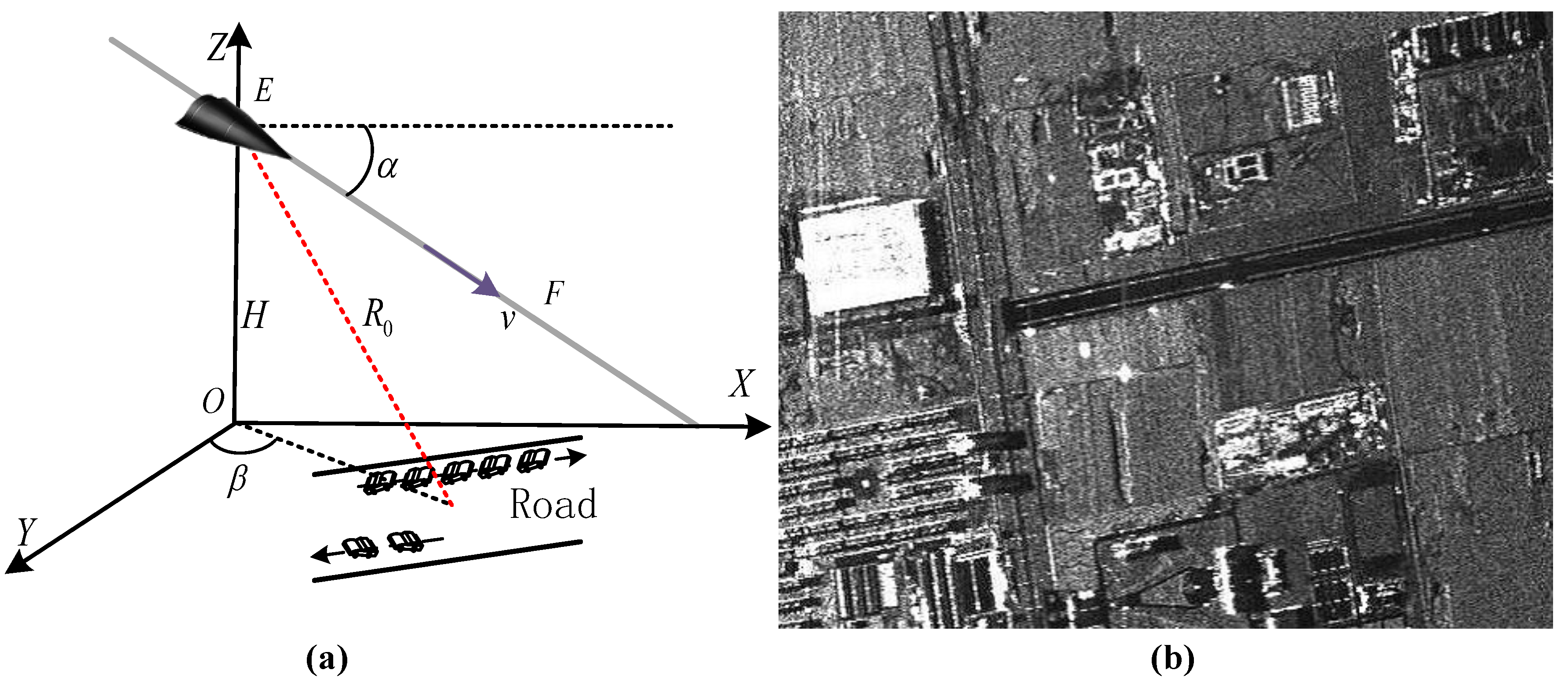
For an HSV, five-sixths of the entire skipping orbit has no acceleration, so we can just focus on a uniform dive orbit [8,9]. Considering a region of interest on the squint side of HSV-SAR with a dive angle , taking a stationary target P as an example, the range model is illustrated in Figure 1. and represent squint angle and slant range. An HSV position is defined with altitude H, synthesized speed v, horizontal speed , and vertical speed . The instantaneous range model for a stationary target [27] can be modeled as
where is the slow-time.
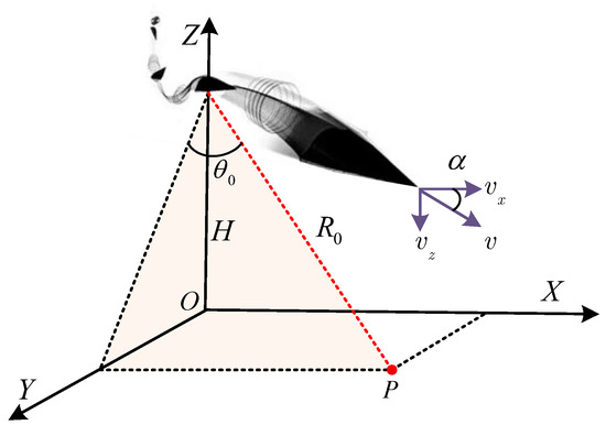
Figure 1.
Geometric model of highly squinted HSV-SAR with a dive orbit for a stationary target.
Figure 2 shows the equivalent model for a stationary target. Equation (1) is simplified to a classic hyperbolic range equation (HRE), and the IERM for a stationary target can be described as
with

Figure 2.
Diagram of equivalent model for a stationary target.
Inspecting (3), the first equation denotes the synthesized speed of the platform, the second equation represents the speed projection operator in the beam center direction, and represents the equivalent squint angle. By utilizing the operator to transform the focusing plane onto Plane DEFP in Figure 2, one guarantees that the impacts of the dive angle can be mitigated. Although the operator simplifies the expression of the range history, there are side effects in the imaging geometry that will be analyzed later.
2.2. IERM for GMT
Taking channel number N as an example, , the data acquisition model of HSV-MC-SAR for a GMT is illustrated in Figure 3, where the data acquisition plane corresponds to the Plane DEFP in Figure 2. The data acquisition model is defined as follows: an arbitrary GMT is denoted by ; the nearest distance between the radar carrier and T is represented by ; the speed vector along the -axis and -axis are denoted by and ; along-track velocity (ATV) and CTV of a GMT are indicated by and ; the adjacent channel distance is represented by d; the distance between the first and the -th channel is denoted by .
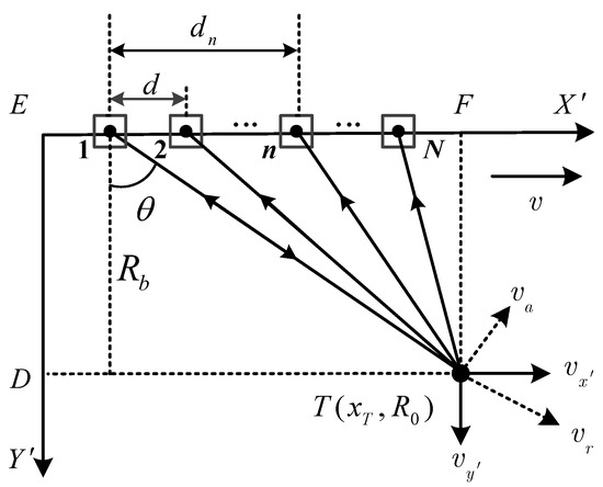
Figure 3.
Data acquisition model for a GMT.
The GMT 2D velocities are introduced as
By extending (4), the range history in the -th channel can be formulated as
where .
From (7), the IERM for a GMT in the -th channel can be modeled as
with
where , and represent the relative ATV and CTV between the radar carrier and T, respectively. Equation (8) enjoys a more concise expression compared to [8], because the dive orbit is transformed into the horizontal orbit. Moreover, its accuracy meets the requirements of high-resolution imageries [7,27].
3. Robust GMTI Scheme for Highly Squint-Looking HSV-MC-SAR in Dive Mode
From Figure 4, the whole flowchart can be grouped into four areas: (1) The coarse imaging using the cubic CFT (CCFT) function, alleviating the impacts of DA and cubic phase. (2) An improved clutter rejection algorithm with a two-step CTV sweep, which has a shorter calculation time because the range of the small-interval sweep is reduced. (3) The GMT finer-imaging algorithm is presented, in combination with the clutter-free signal. (4) By using the inverse projection, the geometry shift of GMT is corrected.
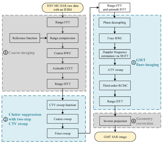
Figure 4.
Flowchart of the proposed scheme.
3.1. Coarsely Imaging
To alleviate the RCM and DA influences, we provide a coarse imaging algorithm in this section with an IERM. After the range Fourier transform (FT) and range compression were accomplished, the received signal in terms of a GMT and the -th channel can be introduced as
where the coefficient represents the complex amplitude of a GMT, c denotes the speed of transmitted linear frequency modulation (LFM) signal, and indicate the range and carrier frequencies, denotes the range-frequency profile, and represents the azimuth-profile. Substituting (8) into (10), yielding
Observing the exponential terms of (11), the second component leads to range walk, the third component results in range curvature, and the fourth component contains the information of third-order RCM.
It is safe to assume that the radar carrier velocity is much greater than the GMT velocity for the HSV-MC-SAR, although the 2D velocities of GMT are typically unknown. The following equivalence relation is reasonable in the coarse imaging stage.
Inspecting (11), the function of coarse range walk correction (RWC) can be constructed as
The influences of the DA and cubic phase make it difficult to focus the GMT. Inspired by square CFT [6,20], the coarse-imaging operator with the CCFT is expressed as
where
The procedure of coarse-imaging is as follows
where denotes the azimuth-frequency profile, the coefficient represents the GMT complex amplitude after azimuth integration, reflects the azimuth CFT frequency, and .
The received signal in the azimuth CFT domain can be written as
where the GMT complex amplitude after range integration is indicated by the coefficients , and the Doppler centroid is denoted by . The number of DA is generally given by , the Doppler bandwidth is represented by , the abbreviation of the pulse repetition frequency is represented as , l is integral, and .
The ambiguity number of Doppler centroid is introduced as
where denotes the maximum integer.
For the baseband received signal, the azimuth frequency, CTV, and Doppler centroid are modeled as
where the first blind velocity is denoted by .
For a GMT, the baseband received signal of the coarse imageries is recovered from (18) and we define
Inspecting (23), the last phase is connected to the channel number, and the GMT steering vector is formulated as
where indicates transpose operation.
From (23), by setting the motion parameter of a GMT to zero, the baseband received signal of stationary clutter in the coarse imageries can be modeled as
Observing (25), the clutter steering vector is introduced as
Inspecting (23) and (25), by sweeping and identifying the maximum output between different ambiguity regions, the ambiguity-free GMT can be retrieved. Since only a few GMTs are present in the region of interest, it can be considered as sparse [7,15,47]. Moreover, the effect of DA stationary clutter may be non-negligible, which will be discussed in the next subsection.
3.2. Improved Clutter Rejection Algorithm with Two-Step CTV Sweep
To reduce the small-interval sweep range of CTV and minimize the effect of DA stationary clutter, an improved clutter rejection algorithm based on a two-step CTV sweep is derived. Furthermore, the cross-track parameter estimation is divided into coarse and small-interval sweeps.
The signal in terms of single-pixel can be introduced as
with
where the range-cell and azimuth-cell indexes of an arbitrary pixel are indicated by p and q.
With the coarse imageries, the geometric model of the joint-pixel is summarized in Figure 5 [15,46]. Furthermore, the reconstructed signal of the joint-pixel can be formulated as follows

Figure 5.
Geometric model of joint-pixel.
The components of the reconstructed signal in (30) are written as
with
where the range-cell and azimuth-cell numbers in the pixel window are represented by and , the range-cell and azimuth-cell indexes in terms of the joint-pixel are indicated by and , the number of pixels in a pixel window is denoted by .
With the linearly constrained minimum-variance (LCMV) [7,15,48], the model is introduced as
where , the optimized steering vector of GMT is represented by , , the array of Kronecker operation is indicated by ⊗, and is the column vector.
The covariance matrix with joint-pixel information in (35) is formulated as [15,46]
where is the sample number, and . and indicate the mean and conjugate transpose operations.
From (35), the weight operator can be generated, viz.,
where the inverting operation is represented by .
The CTV sweep function can be modeled as
where the finer CTV is indicated by , the GMT ambiguity-free region is denoted by , and the optimized weight operator is represented by .
The clutter elimination processors can be introduced as
The clutter rejection processors for different algorithms are shown in Figure 6, where the dotted line on the left denotes the general Doppler spectrum diagram (DSD) [7,49] of a GMT and clutter. T-point, C-point, and -point denote a GMT, clutter, and a DA component of clutter. The green and orange parallelograms represent an arbitrary ambiguity region and the GMT ambiguity-free region, respectively. M-point, which is the midpoint of dashed line , represents the assumed GMT. A GMT can be obtained through placing the zeros in the DA clutter directions, because the GMT is sparse for the coarse-imaging imageries [7,15]. The CFT-center algorithm locates the beamforming center in the assumed GMT direction, and the CFT-two-step algorithm steers the beamforming center as determined by the coarse CTV—they both have beamforming mismatch. The proposed algorithm, which has the matched beamforming in the GMT direction, enhances the SCNR and forms the basis for reducing the GMTI processing.
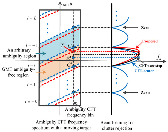
Figure 6.
Clutter rejection processors for our proposed algorithm and other algorithms.
Next, we shall introduce the CTV estimation based on the two-step sweep, and the process can be described as follows:
- CTV estimation with the large-interval sweep. (a) Coarse sweeping in an arbitrary region. Perform the large-interval sweep with the sweep function of (38) in the l-th ambiguity region. (b). Repeat (a) for all ambiguity regions. By sweeping and identifying the maximum output between different ambiguity regions, the GMT true region can be retrieved. (c). Determine the small-interval sweep range. The small-interval sweep range can be determined from the best and second best CTV values generated by large-interval sweep in the GMT ambiguity-free region.
- CTV estimation with the small-interval sweep. Sweeping in the small-interval sweep range, the finer CTV can be estimated from the output that maintains the maximum GMT power.
3.3. GMT Finer-Imaging
After the aforementioned processing, GMT together with the accurate CTV can be obtained. Here, a GMT finer-imaging algorithm for the highly squinted HSV-MC-SAR with a dive orbit is derived, ATV estimated and the GMT velocities revised. Compared to the CFT-two-step algorithm [6], the proposed GMT finer-imaging algorithm preprocesses the swept CTV and its RWC operator is reduced to a single-step operation.
Transforming the received signal into the range frequency domain, yielding
with
where an arbitrary is denoted by , the aperture center time for the GMT is expressed by .
Taking the second-order Keystone Transform (SOKT) [6,7,8,15,50,51], the coupling between range frequency and square term of slow-time can be minimized, and its transform operator is introduced as
where represents the transformed slow-time.
The range frequency is much smaller than carrier frequency, and thus the following expression is reasonable, viz.,
Observing (45), the coupling between range frequency and square term of slow-time is eliminated, and it is easy to obtain the finer RWC operator and yields
With the finer RWC operator, the received signal can be generated as
After that, we reconstruct the second-order phase and yield
with
Transforming (48) into the 2D time domains, that is,
The processing of simplified fractional Fourier transform (SFrFT) [52,53] is described as
where the kernel operator is introduced as [54]. The rotation factor is recovered by sweeping the maximum power of (51), that is [55]
The ATV sweep of GMT can hence be modeled as
where reflects the chirp rate of the received signal, and indicates the sampling number in the slow-time direction.
In order to realize the GMT finer-imaging, with the swept parameter in (38) and (53), the operators of azimuth matched filtering and third-order range cell migration correction (RCMC) can be generated.
where illustrates the transformed version of frequency corresponding to the transformed slow-time.
3.4. Geometry Correction
With the aforementioned operation, we apply an IERM to achieve the GMTI for the highly squinted HSV-MC-SAR with a dive orbit. Although the speed projection operator (e.g., range model equivalence) simplifies the entire GMTI process, its side effect is geometry shift. Utilizing the operator to transform the focusing plane onto Plane DEFP, the geometry shift is more serious compared to the classic focusing model, as shown in Figure 7. The inverse projection is an effective tool to mitigate the shift induced by the vertical speed of HSV [27,56]. The first step of the tool is to place a uniform alignment grid on the ground, and the second step is to project a GMT to the Plane DEFP. From Figure 7, is the azimuth angle, the following relation between and can be modeled as
with
where the Doppler frequency of the target on the ground is represented by .
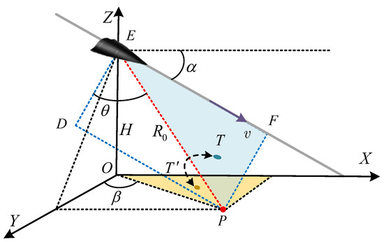
Figure 7.
Formulation of geometric correction.
4. Simulations and Examples
4.1. Point Targets
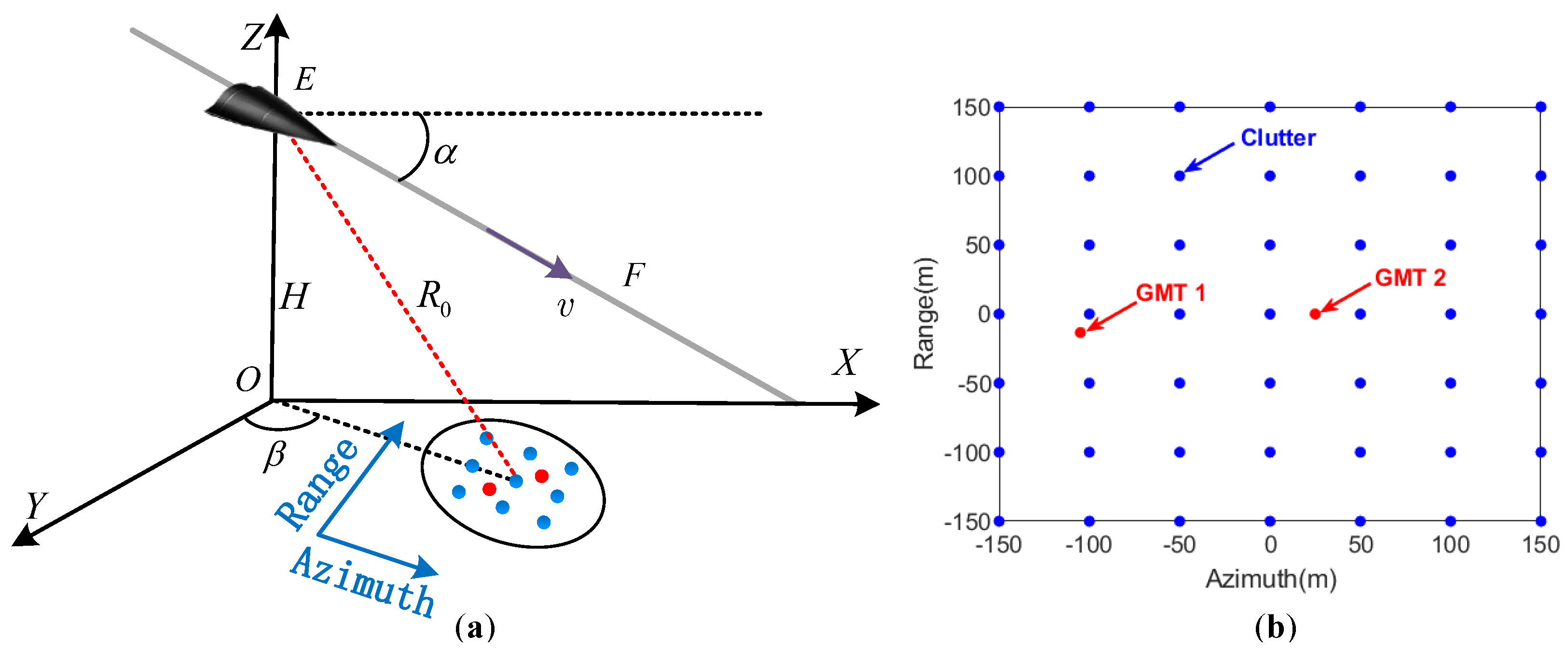
In order to demonstrate the effectiveness of the proposed scheme for the highly squinted HSV-MC-SAR with a dive trajetory, the simulation results of point targets are provided and the simulation parameters are shown in Table 1. We consider a scattering point model comprising a 0 dB signal-to-clutter ratio (SCR) and 10 dB signal-to-noise ratio (SNR), and the geometric configuration is depicted in Figure 8. The ATV and CTV of the first GMT are, respectively, 8 and 8 m/s, and of the second GMT are 0 and 8 m/s.

Table 1.
Simulation parameters.
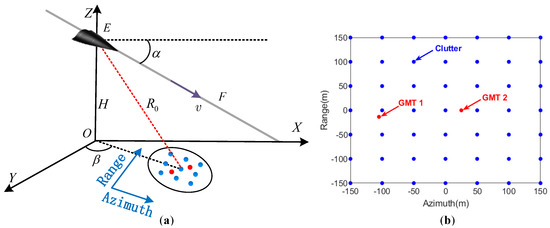
Figure 8.
Geometric configuration of point targets. (a) Geometric configuration. (b) The point targets on the ground.
First, we provide the results after range compression as shown in Figure 9a without the coarse RWC, and in Figure 9b with the coarse RWC. It is noted that the point target envelopes are basically straightened after the coarse RWC.
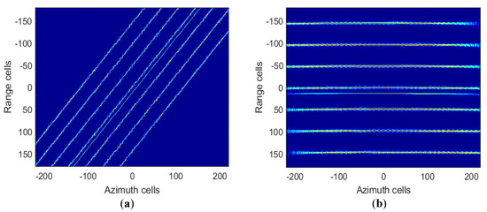
Figure 9.
The results after range compression. (a) Without the coarse RWC. (b) With the coarse RWC.
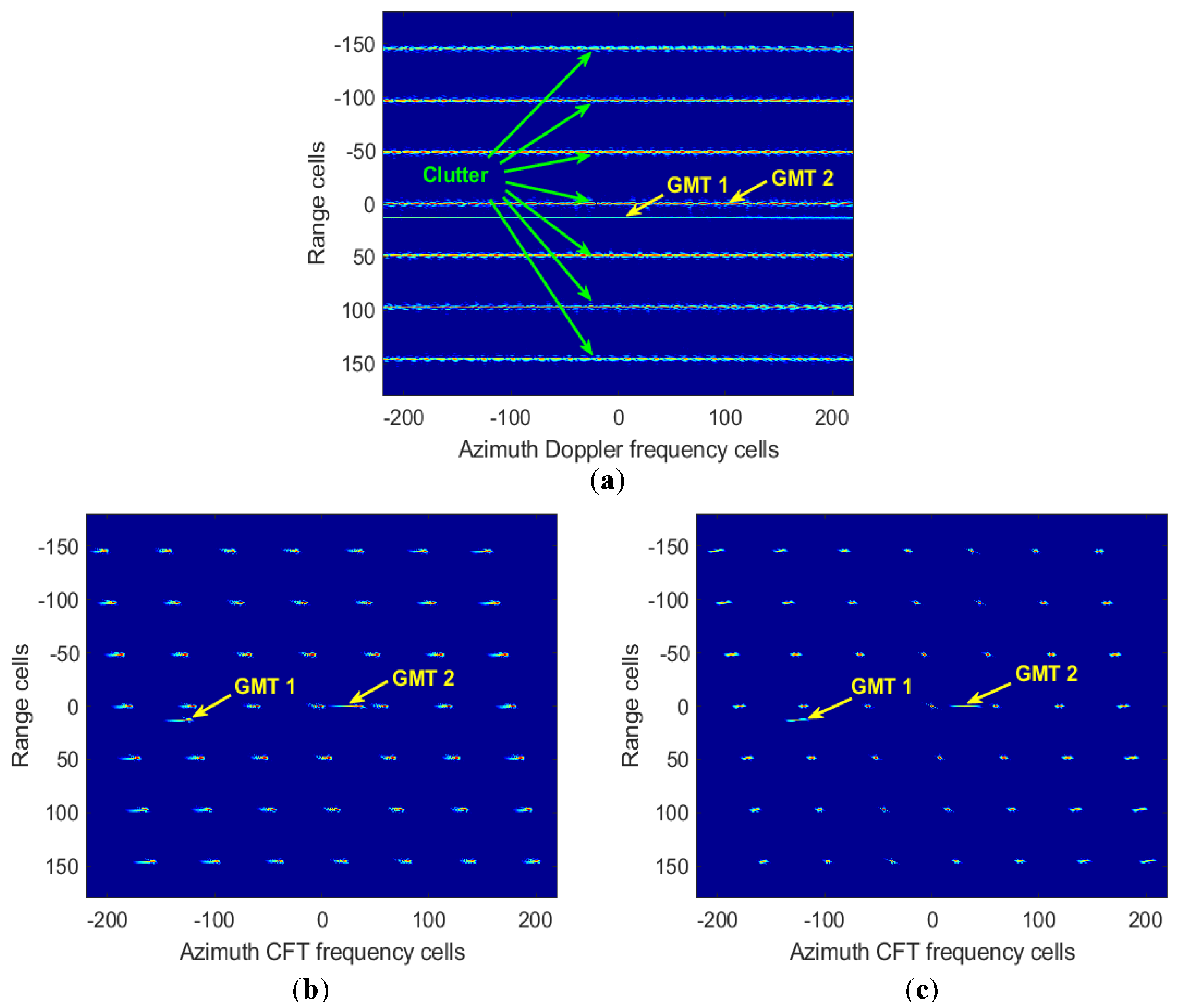
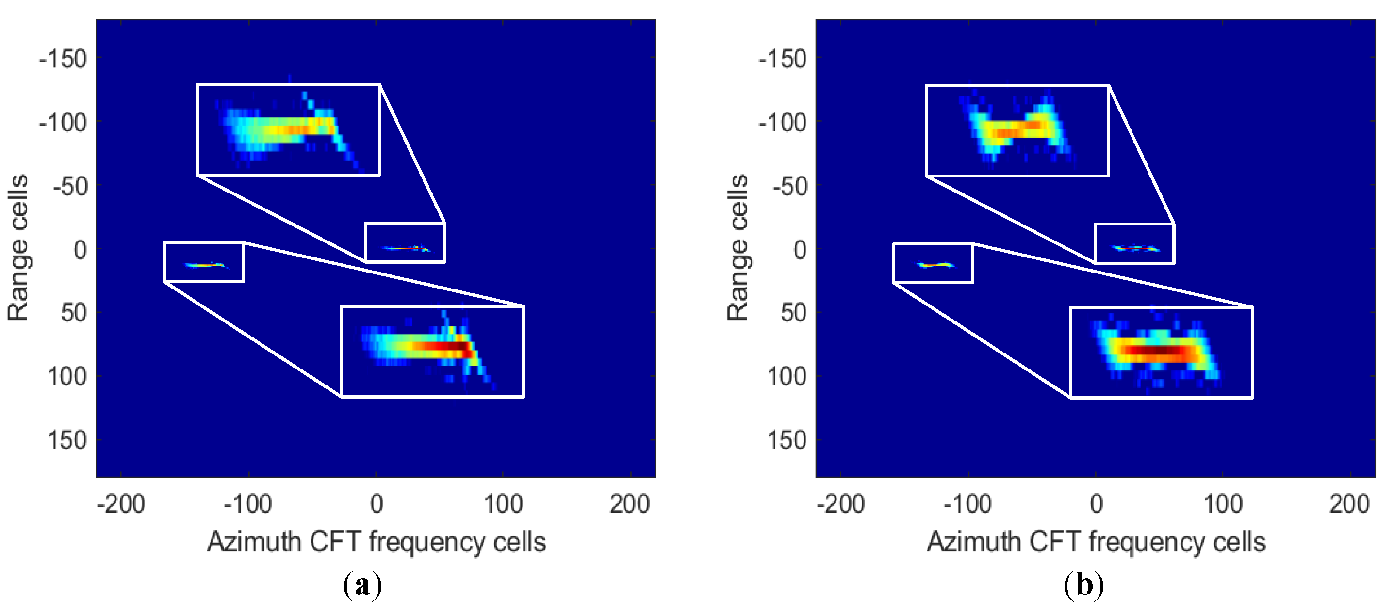
Then, the coarse-focusing images of point targets are illustrated in Figure 10. The envelopes of point targets with azimuth FT are shown in Figure 10a, and one notices that the second GMT overlaps with the clutter. Figure 10b,c represents the coarse-imaging results, coarsely focusing image with the square CFT and coarsely focusing image with CCFT. One can notice that all point targets are roughly focused and the GMTs are now distinguished from the clutter. Moreover, the CCFT, which compensates for the high-order phase terms, outperforms the square CFT in the coarse-focusing of point targets. Applying inverse projection to revise the geometry shift in Figure 10c, the “square imagery” is yielded as shown in Figure 11, where the imagery corresponds to the distribution of point targets in Figure 8b.

Figure 10.
The coarse-focusing images. (a) Azimuth FT. (b) Azimuth square CFT. (c) Azimuth CCFT.
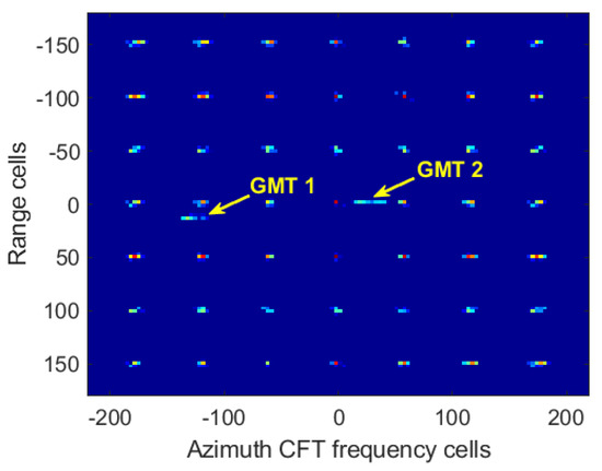
Figure 11.
The geometry correction results for the coarse-focusing images.
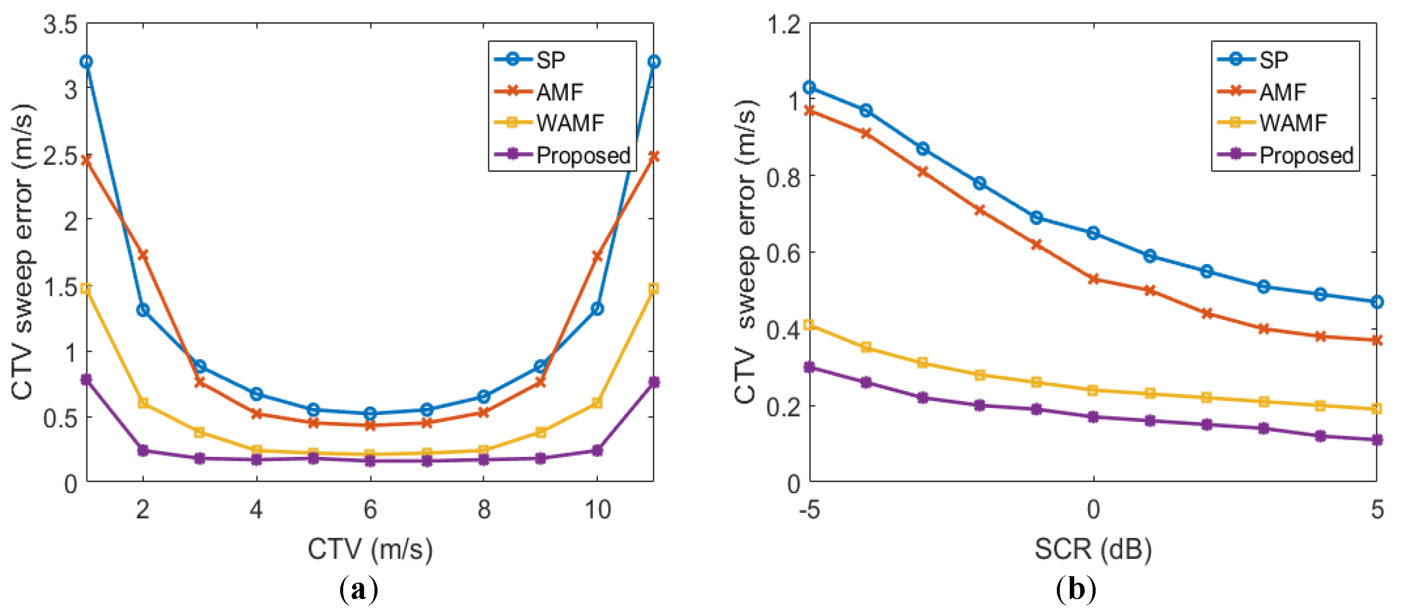
Figure 12a illustrates the CTV sweep errors for different algorithms with respect to different CTV. One can see that the proposed CTV sweep algorithm obtains less error compared to the other algorithms. When faced with DA and phase errors, the other algorithms run into degradation of CTV sweep. The performance of the CTV sweep will drop when CTV is close to an integer multiple of the first blind velocity, because the GMT and clutter have close azimuth Doppler frequency and are difficult to distinguish. Figure 12b shows the errors of the CTV sweep with , and the performance of the CTV sweep becomes better as the SCR increases.
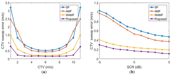
Figure 12.
The errors of CTV sweep for different algorithms. (a) With different CTV. (b) With different SCR.
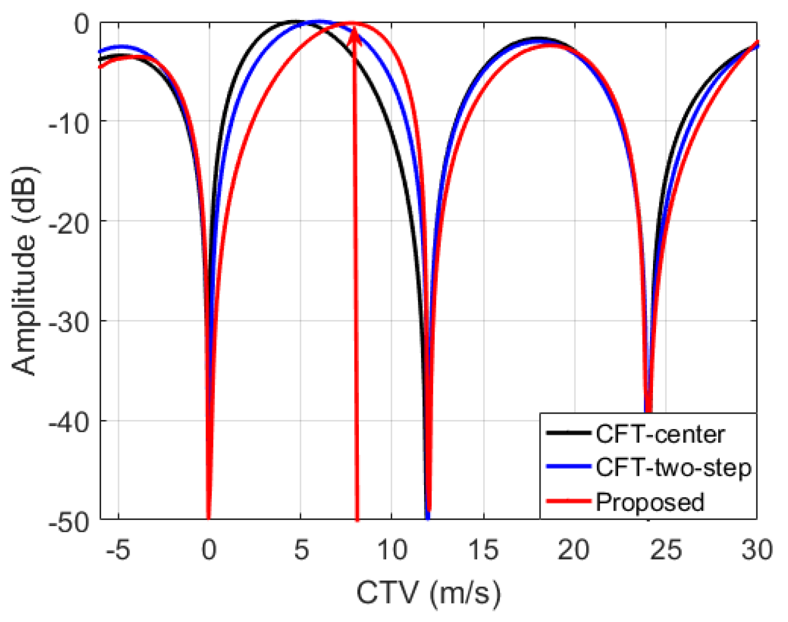
Figure 13 shows the beamforming for the proposed and the other algorithms, and the red arrow represents the true CTV of a GMT. The results show that the proposed algorithm has the highest amplitude in the red arrow direction compared with the other algorithms. Due to the lack of swept CTV for the CFT-center and CFT-two-step algorithms in this stage, they generate the beams that do not match a GMT. Fortunately, the proposed algorithm generates a matched beamforming by swept CTV.

Figure 13.
Beamforming for different algorithms.
After clutter rejection, the images are as shown in Figure 14, where the white rectangular areas represent the enlarged image of the GMT profiles. With the square CFT [6,20], the GMT images are smeared due to the inevitable third-order phase, as illustrated in Figure 14a. As shown in Figure 14b, the proposed scheme obtains better GMT envelopes because the third-order phase is corrected by CCFT and matched beamforming is generated from swept CTV [7,15].

Figure 14.
The images after clutter rejection. (a) Azimuth square CFT. (b) Azimuth CCFT.
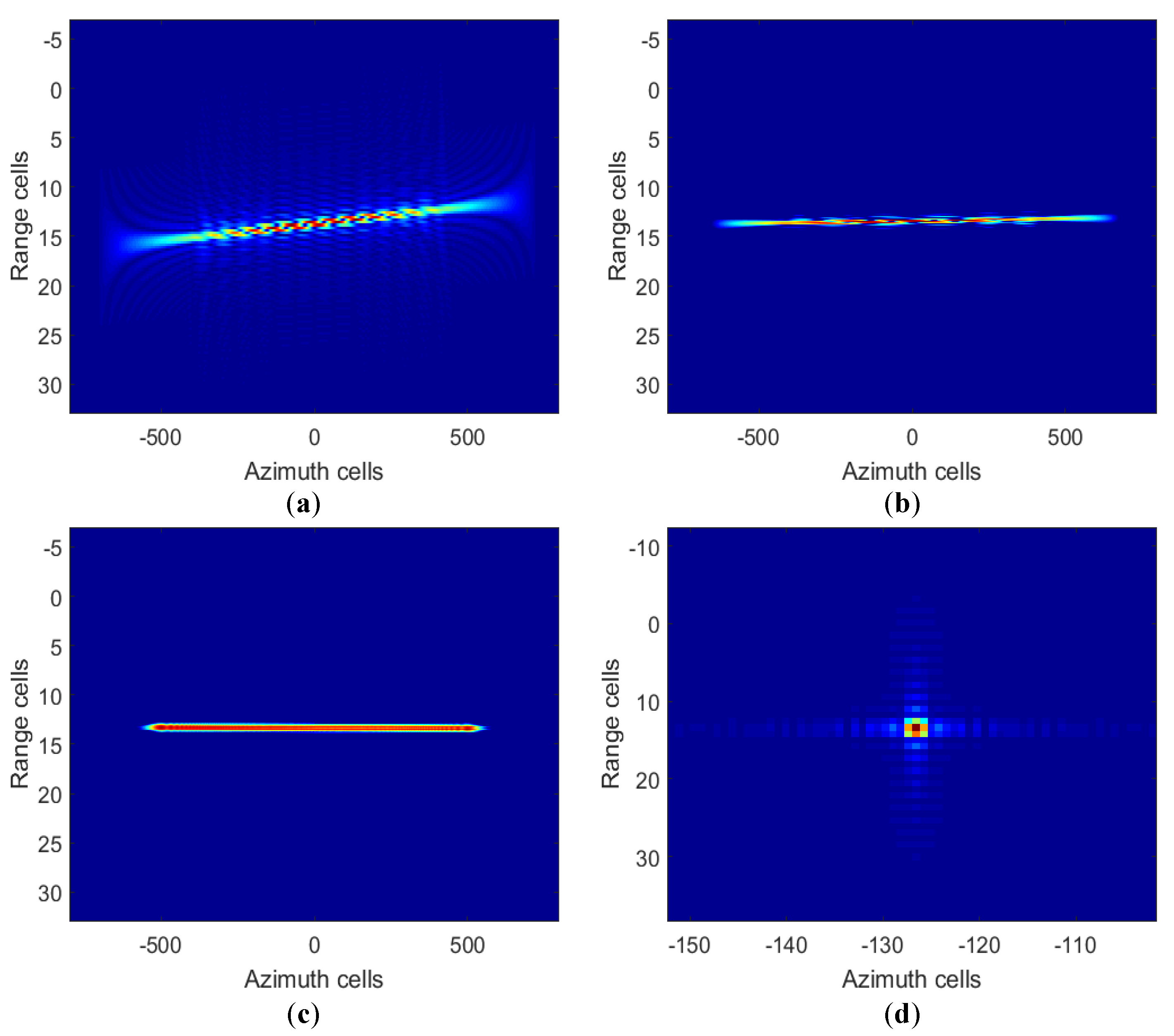
After that, the finer-imaging processing for the first GMT is shown in Figure 15. Transforming the received signal into the time domain, its misaligned envelope is shown in Figure 15a. The image obtained is shown in Figure 15b with SOKT and shown in Figure 15c with finer RWC. One can see that the straightened envelope of the first GMT is retrieved. After third-order RCMC and geometry correction, the sidelobe of the first GMT and geometry shift are inhibited, and the finer-imaging GMT image is recovered, as shown in Figure 15d.

Figure 15.
The finer-imaging processing for the first GMT. After (a) coarse imaging, (b) SOKT, (c) finer RWC, and (d) third-order RCMC plus geometry correction.
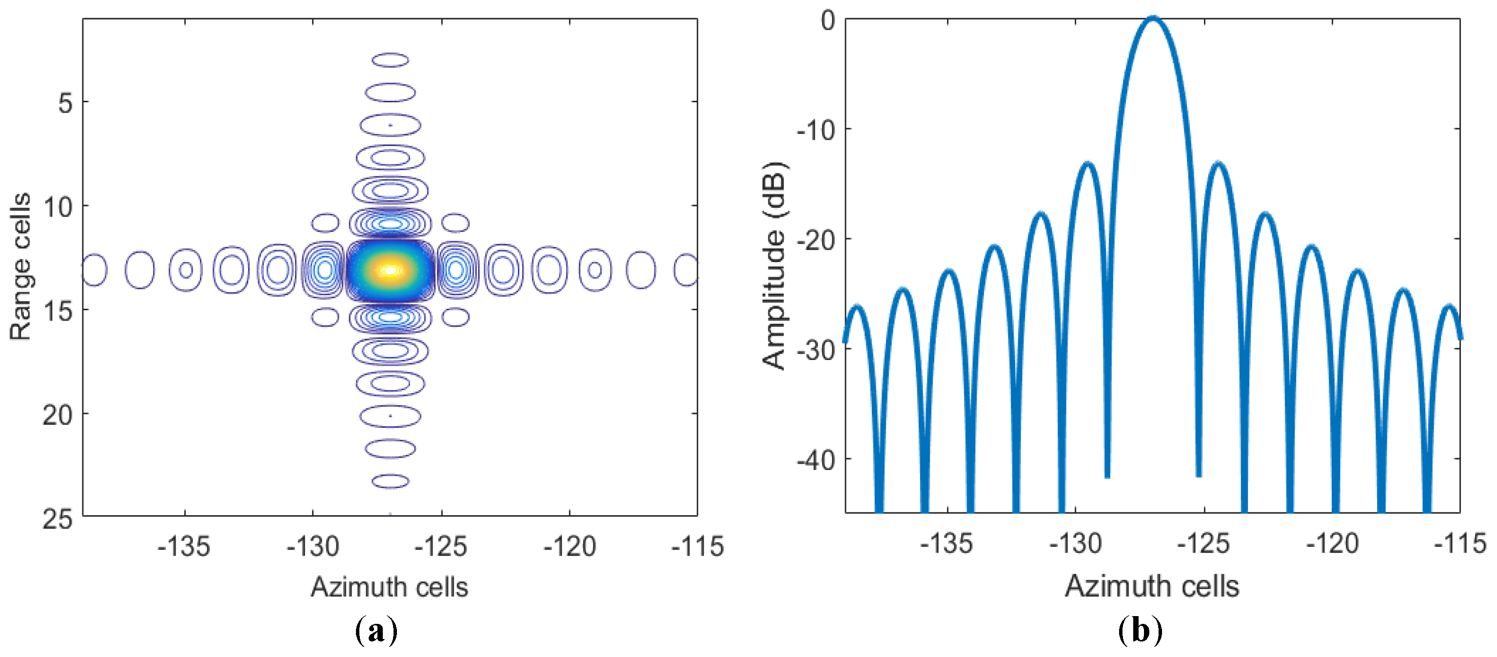
Finally, we further evaluated the finer-imaging result of the first GMT in Figure 15d, the contour plots are shown in Figure 16. The 2D contour plots are shown in Figure 16a, where the main-lobes and sidelobes are not coupled or “crossed”. We consider the evaluation index comprising −13.27 dB at the ideal peak sidelobe ratio (PSLR) and −10.24 dB at the ideal integrated sidelobe ratio (ISLR). The azimuth slice of 2D contour plots is shown in Figure 16b, where the PSLR and ISLR are, respectively, −13.14 and −10.15 dB, which are close to the ideal values.
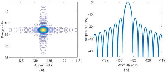
Figure 16.
The evaluation of the finer-imaging result for the first GMT. (a) 2D contour plots. (b) Azimuth slice.
In order to compare the proposed algorithm with existing algorithms, the results are shown in Table 2. It can be seen that the proposed algorithm has the highest SCNR compared to the other algorithms. The reason is that the ISTAP algorithm suffers degradation of energy accumulation due to the insufficient channel numbers of the HSV-SAR. The CFT-center algorithm locates the beamforming center in the assumed GMT direction, and the CFT-two-step algorithm steers the beamforming center as determined by the coarse CTV, they both have beamforming mismatch and energy loss. On the other hand, the proposed algorithm has the best performance of GMT 2D velocity sweep compared to the other algorithms. During clutter suppression, the CFT-center algorithm does not sweep for CTV and the CFT-two-step algorithm achieves only a coarse CTV sweep. More importantly, the performance of parameter sweep becomes better as the SCNR increases.
Table 2.
Performance for different algorithms.
The algorithm complexities of primary steps for different algorithms are listed in Table 3, where the consumption time is mainly determined by clutter rejection. The ISTAP algorithm performs clutter rejection with 2D velocity sweep and is computationally time-consuming. The proposed algorithm, due to the smaller range of small-interval sweep, has a shorter calculation time compared to the CFT-modified algorithm. While the complexities of the proposed algorithm are slightly higher than the CFT-center and CFT-two-step algorithms, the 2D velocity sweep is more accurate, beamforming is better matched, and extracted GMT energy is stronger.
Table 3.
Complexity for different algorithms.
In Table 3, the sweep numbers of ATV and CTV are represented by and , the range pluses and the large-interval sweep number of CTV are represented by and . The phase decoupling with SOKT consumes multiplications and additions. The ATV sweep with SFrFT costs multiplications and additions. The RWC with the efficient Radon transform estimation (ERTE) requires multiplications and additions [6]. It is assumed that the above five algorithms have the same complexities for the GMT finer-imaging, without counting the parameter estimation and phase decoupling.
4.2. Surface Targets
In this section, we evaluate the performance of the proposed algorithm by simulating the imaging of a surface moving target. The simulation parameters are listed in Table 1. The geometric configuration of a surface target is sketched in Figure 17. The surface moving target is a car that has m/s and m/s.
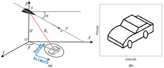
Figure 17.
Geometric configuration of surface targets. (a) Geometric configuration. (b) A surface target on the ground.
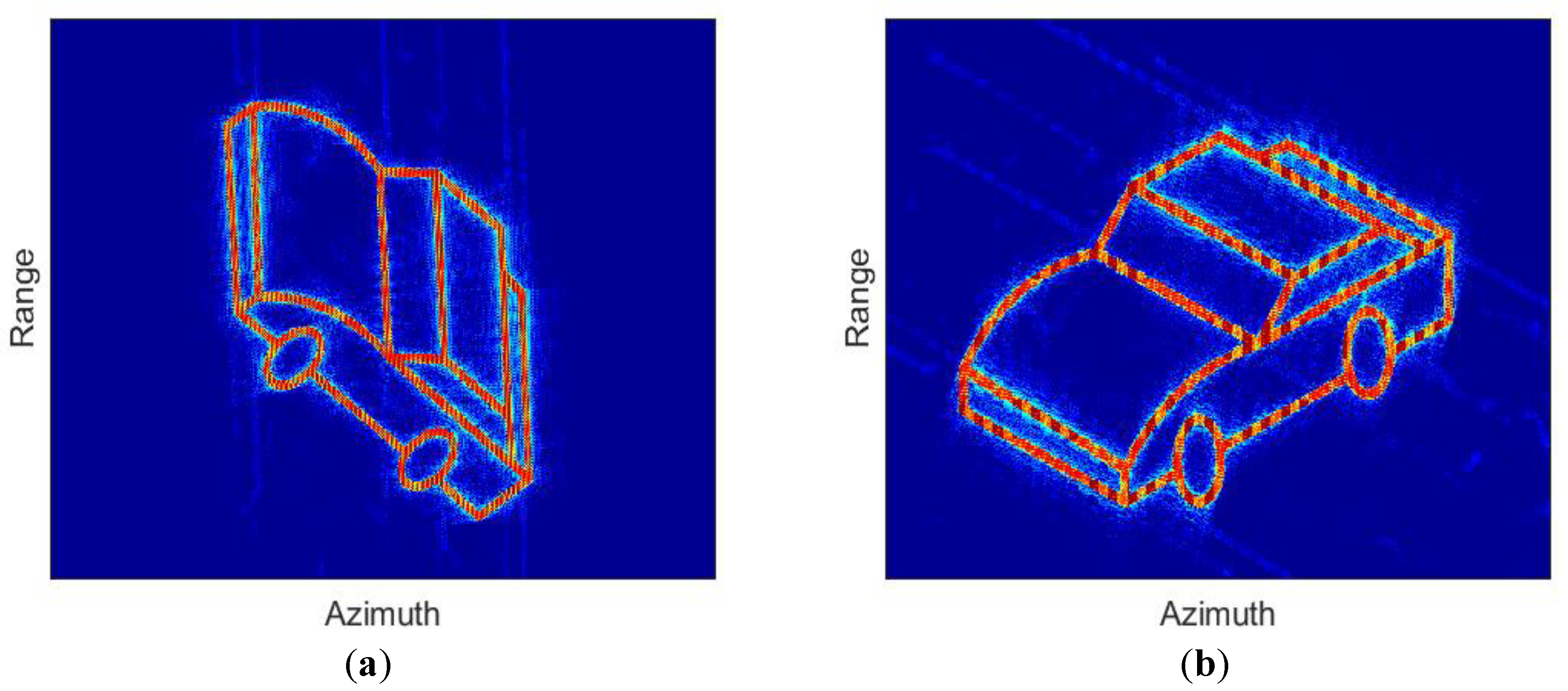
The finer-imaging results after the proposed scheme was accomplished are shown in Figure 18a. Although the focused image of a vehicle is satisfactory, the geometry shift induced by the vertical speed is present. After geometry correction, the geometry shift is revised and the result is as illustrated in Figure 18b, very close to that sketched in Figure 17b. Therefore, the GMT finer-imaging and geometry correction of the proposed scheme are feasible.

Figure 18.
The finer-imaging result. (a) Before geometry correction. (b) After geometry correction.
4.3. Multiple Targets and Extended Scene
In this section, we evaluate the performance of the proposed algorithm by simulating the SAR imaging and localization of multiple targets. Figure 19a shows seven vehicles driving on a road in the region of interest. These simulated targets are then superimposed on the SAR image obtained by air-borne X-band multichannel SAR (MC-SAR), as illustrated in Figure 19b.

Figure 19.
Geometric configuration. (a) The target configuration. (b) The scene configuration.
Figure 20a shows the finer-imaging results, one can see that the geometry shift induced by the vertical speed is present. Figure 20b illustrates the localization results after geometry correction, where the yellow and red marks represent the location and relocation results of the targets. We notice the scene is very close to that sketched in Figure 19b where the targets are marked on or beside the road. Therefore, the finer-imaging and target localization of the proposed scheme are effective.
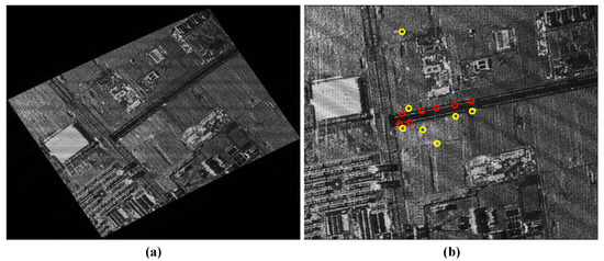
Figure 20.
The processing result. (a) The finer-imaging result before geometry correction. (b) The localization result after geometry correction.
5. Conclusions
Existing researches of HSV-SAR/GMT indication (GMTI) focus their region of interest on side-looking mode or squinted mode with a horizontal orbit. The proposed GMTI scheme for HSV-MC-SAR is new and focuses the region of interested on the high-squint side of a dive orbit. At first, an IERM, which provides a concise expression and simplifies the GMTI process, is explored. Then, a robust clutter rejection and GMT imaging algorithm for the highly squinted HSV-MC-SAR with a dive orbit is derived in detail, incorporated with the IERM model. Finally, the geometry shift of GMT is revised by inverse projection. Compared with the existing researches, the proposed scheme has accurate recoveries of GMT 2D speeds, matched beamforming, and satisfactory GMTI performance.
Author Contributions
J.H. and Y.C. developed the theory and signal model. J.H. and W.W. performed and analyzed the numerical simulations. J.H., Y.W., T.-S.Y., S.L. and F.W. wrote and edited the paper. All authors have read and agreed to the published version of the manuscript.
Funding
This work was funded by the National Nature Science Foundation of China under Grant 61771367 and in part by the Science and Technology on Communication Networks Laboratory under Grant 6142104190204, as well as in part by the 111 Project under Grant B18039.
Conflicts of Interest
The authors declare no conflict of interest.
References
- Kang, M.-S.; Kim, K.-T. Ground moving target imaging based on compressive sensing framework with single-channel SAR. IEEE Sens. J. 2020, 20, 1238–1250. [Google Scholar] [CrossRef]
- Wang, W. Near-space vehicle-borne SAR with reflection-antenna for high-resolution and wide-swath remote sensing. IEEE Trans. Geosci. Remote Sens. 2012, 50, 338–348. [Google Scholar] [CrossRef]
- Kang, M.-S.; Won, Y.-J.; Lim, B.-G.; Kim, K.-T. Efficient synthesis of antenna pattern using improved PSO for spaceborne SAR performance and imaging in presence of element failure. IEEE Sens. J. 2018, 18, 6576–6587. [Google Scholar] [CrossRef]
- Khedkar, S.B.; Kasav, S.M.; Khedkar, A.S.; Mahajan, S.M.; Satpute, D.R. A Review on Hypersonic Aircraft. Int. J. Adv. Technol. Eng. Sci. 2015, 3, 1566–1570. [Google Scholar]
- Xu, X.; Liao, G.; Yang, Z.; Wang, C. Moving-in-pulse duration model-based target integration method for HSV-borne high-resolution radar. Digit. Signal Process. 2017, 68, 31–43. [Google Scholar] [CrossRef]
- Wang, Y.; Cao, Y.; Wang, S.; Su, H. Clutter Suppression and Ground Moving Target Imaging Approach for Hypersonic Vehicle borne multichannel radar based on Two-Step focusing Method. Digit. Signal Process. 2019, 85, 62–76. [Google Scholar] [CrossRef]
- Han, J.; Cao, Y.; Yeo, T.S.; Wang, F.; Liu, S. A novel hypersonic vehicle-borne multichannel SAR-GMTI scheme based on adaptive sum and difference beams within eigenspace. Signal Process. 2021, 187, 108168. [Google Scholar] [CrossRef]
- Wang, Y.; Cao, Y.; Peng, Z.; Su, H. Clutter suppression and moving target imaging approach for multichannel hypersonic vehicle borne radar. Digit. Signal Process. 2017, 68, 81–92. [Google Scholar] [CrossRef]
- Carter, P.H., II; Pines, D.J.; Rudd, L.V. Approximate Performance of Stageic Hypersonic Trajectories for Global Reach. IBM J. Res. Dev. 2000, 44, 703–714. [Google Scholar] [CrossRef]
- Kang, M.-S.; Bae, J.-H.; Kang, B.-S.; Kim, K.-T. ISAR cross-range scaling using iterative processing via principal component analysis and bisection algorithm. IEEE Trans. Signal Process. 2016, 64, 3909–3918. [Google Scholar] [CrossRef]
- Kang, M.-S.; Bae, J.-H.; Lee, S.-H.; Kim, K.-T. Efficient ISAR autofocus via minimization of Tsallis Entropy. IEEE Trans. Aerosp. Electron. Syst. 2016, 52, 2950–2960. [Google Scholar] [CrossRef]
- Kang, M.-S.; Kang, B.-S.; Lee, S.-H.; Kim, K.-T. Bistatic-ISAR distortion correction and range and cross-range scaling. IEEE Sens. J. 2017, 17, 5068–5078. [Google Scholar] [CrossRef]
- Tang, S.; Guo, P.; Zhang, L.; So, H.C. Focusing Hypersonic Vehicle-Borne SAR Data Using Radius/Angle Algorithm. IEEE Trans. Geosci. Remote Sens. 2020, 58, 281–293. [Google Scholar] [CrossRef]
- Chen, Z.; Zhou, Y.; Zhang, L.; Lin, C.; Huang, Y.; Tang, S. Ground Moving Target Imaging and Analysis for Near-Space Hypersonic Vehicle-Borne Synthetic Aperture Radar System with Squint Angle. Remote Sens. 2018, 10, 1966. [Google Scholar] [CrossRef] [Green Version]
- Han, J.; Cao, Y.; Yeo, T.S.; Wang, F. Robust Clutter Suppression and Ground Moving Target Imaging Method for a Multichannel SAR with High-Squint Angle Mounted on Hypersonic Vehicle. Remote Sens. 2021, 13, 2051. [Google Scholar] [CrossRef]
- Zhang, S.; Xing, M. A Novel Doppler Chirp Rate and Baseline Estimation Approach in the Time Domain Based on Weighted Local Maximum-Likelihood for an MC-HRWS SAR System. IEEE Trans. Geosci. Remote Sens. Lett. 2017, 14, 299–303. [Google Scholar] [CrossRef]
- Xu, J.; Huang, Z.; Wang, Z.; Xiao, L.; Xia, X.; Long, T. Radial Velocity Retrieval for Multichannel SAR Moving Targets With Time–Space Doppler Deambiguity. IEEE Trans. Geosci. Remote Sens. 2018, 56, 35–48. [Google Scholar] [CrossRef]
- Lv, G.; Li, Y.; Wang, G.; Zhang, Y. Ground Moving Target Indication in SAR Images With Symmetric Doppler Views. IEEE Trans. Geosci. Remote Sens. 2016, 54, 533–543. [Google Scholar] [CrossRef]
- Huang, Y.; Liao, G.; Xu, J.; Yang, D. MIMO SAR OFDM chirp waveform design and GMTI with RPCA based method. Digit. Signal Process. 2016, 51, 184–195. [Google Scholar] [CrossRef]
- Zhang, S.; Xing, M.; Xia, X. Robust clutter suppression and moving target imaging approach for multichannel in azimuth high-resolution and wide-swath synthetic aperture radar. IEEE Trans. Geosci. Remote Sens. 2015, 53, 687–709. [Google Scholar] [CrossRef]
- Eldhuset, K. A new fourth-order processing algorithm for spaceborne SAR. IEEE Trans. Aerosp. Electron. Syst. 1998, 34, 824–835. [Google Scholar] [CrossRef] [Green Version]
- Luo, Y.; Zhao, B.; Han, X.; Wang, R.; Song, H.; Deng, Y. A novel high-order range model and imaging approach for highresolution LEO SAR. IEEE Trans. Geosci. Remote Sens. 2014, 52, 3473–3485. [Google Scholar] [CrossRef]
- Huang, L.; Qiu, X.; Hu, D.; Ding, C. Focusing of medium-earth-orbit SAR with advanced nonlinear chirp scaling algorithm. IEEE Trans. Geosci. Remote Sens. 2011, 49, 500–508. [Google Scholar] [CrossRef]
- Bao, M.; Xing, M.; Wang, Y.; Li, Y. Two-dimensional spectrum for MEO SAR processing using a modified advanced hyperbolic range equation. Electron. Lett. 2011, 47, 1043–1045. [Google Scholar] [CrossRef]
- Li, Z.; Yi, L.; Xing, M.; Huai, Y.; Gao, Y.; Zeng, L.; Bao, Z. An improved range model and omega-K-based imaging algorithm for high-squint SAR with curved orbit and constant acceleration. IEEE Geosci. Remote Sens. Lett. 2016, 13, 656–660. [Google Scholar] [CrossRef]
- Wang, P.; Liu, W.; Chen, J.; Niu, M.; Yang, W. A high-order imaging algorithm for high-resolution spaceborne SAR based on a modified equivalent squint range model. IEEE Geosci. Remote Sens. 2015, 53, 1225–1235. [Google Scholar] [CrossRef] [Green Version]
- Li, Z.; Xing, M.; Xing, W.; Liang, Y.; Gao, Y.; Dai, B.; Bao, Z. A Modified Equivalent Range Model and Wavenumber-Domain Imaging Approach for High-Resolution-High-Squint SAR With Curved Trajectory. IEEE Geosci. Remote Sens. 2017, 55, 3721–3734. [Google Scholar] [CrossRef]
- Makhoul, E.; Broquetas, A.; Rodon, J.R.; Zhan, Y.; Ceba, F. A performance evaluation of sar-gmti missions for maritime applications. IEEE Trans. Geosci. Remote Sens. 2015, 53, 2496–2509. [Google Scholar] [CrossRef] [Green Version]
- Faubert, D.; Tam, W. Improvement in the detection performance of a space based radar using a displaced phase centre antenna. In Proceedings of the 1987 Antennas and Propagation Society International Symposium, Blacksburg, VA, USA, 15–19 June 1987; pp. 964–967. [Google Scholar]
- Lightstone, L.; Faubert, D.; Rempel, G. Multiple phase centre DPCA for airborne radar. In Proceedings of the 1991 IEEE National Radar Conference, Los Angeles, CA, USA, 12–13 March 1991; pp. 36–40. [Google Scholar]
- Klemm, R. Introduction to space-time adaptive processing. Electron. Commun. Eng. J. 1999, 11, 5–12. [Google Scholar] [CrossRef]
- Xu, L.; Gianelli, C.; Jian, L. Long-CPI multichannel SAR-based ground moving target indication. IEEE Trans. Geosci. Remote Sens. 2016, 54, 5159–5170. [Google Scholar] [CrossRef]
- Huang, Y.; Liao, G.; Xu, J.; Li, J.; Yang, D. GMTI and Parameter Estimation for MIMO SAR System via Fast Interferometry RPCA Method. IEEE Trans. Geosci. Remote Sens. 2018, 56, 1174–1187. [Google Scholar] [CrossRef]
- Wang, Y.; Cao, Y.; Peng, Z. Clutter suppression and GMTI for hypersonic vehicle borne SAR system with MIMO antenna. IET Signal Process. 2017, 11, 909–915. [Google Scholar] [CrossRef]
- Maori, D.C.; Sikaneta, I. A generalization of DPCA processing for multichannel SAR/GMTI radars. IEEE Trans. Geosci. Remote Sens. 2013, 51, 560–572. [Google Scholar] [CrossRef]
- Delphine, C.; Ishuwa, S. Optimum GMTI processing for space-based SAR/GMTI systems—Theoretical derivation. In Proceedings of the 8th European Conference on Synthetic Aperture Radar, Aachen, Germany, 7–10 June 2010; pp. 390–393. [Google Scholar]
- Makhoul, E.; Broquetas, A.; Gonzalez, O. Evaluation of state-ofthe- art GMTI techniques for future space-borne SAR system-simulation validation. In Proceedings of the 9th European Conference on Synthetic Aperture Radar (EUSAR 2012), Nuremberg, Germany, 23–26 April 2012; pp. 376–379. [Google Scholar]
- Cerutti-Maori, D.; Sikaneta, I.C.H. Gierull, Optimum SAR/GMTI Processing and Its Application to the Radar Satellite RADARSAT-2 for Traffic Monitoring. IEEE Trans. Geosci. Remote Sens. 2012, 50, 3868–3881. [Google Scholar] [CrossRef]
- Li, X.; Xing, M.; Xia, X.; Sun, G.; Yi, L.; Zheng, B. Deramp space-time adaptive processing for multichannel SAR systems. IEEE Trans. Geosci. Remote Sens. Lett. 2014, 11, 1448–1452. [Google Scholar]
- Huang, Y.; Liao, G.; Xu, J.; Li, J. GMTI and Parameter Estimation via Time-Doppler Chirp-Varying Approach for Single-Channel Airborne SAR System. IEEE Trans. Geosci. Remote Sens. 2017, 55, 4367–4383. [Google Scholar] [CrossRef]
- Rousseau, L.; Gierull, C.; Chouinard, J. First results from an experimental ScanSAR-GMTI mode on RADARSAT-2. IEEE J. Sel. Topics Appl. Earth Observ. Remote Sens. 2015, 8, 5068–5080. [Google Scholar] [CrossRef]
- Zhang, S.; Zhou, F.; Sun, G.; Xia, X.; Bao, Z. A new SAR-GMTI high-accuracy focusing and relocation algorithm using instantaneous interferometry. IEEE Trans. Geosci. Remote Sens. 2016, 54, 5564–5577. [Google Scholar] [CrossRef]
- Dragosevic, M.V.; Burwash, W.; Chiu, S. Detection and estimation with RADARSAT-2 moving-object detection experiment modes. IEEE Trans. Geosci. Remote Sens. 2012, 50, 3527–3543. [Google Scholar] [CrossRef]
- Robey, F.C.; Fuhrmann, D.R.; Kelly, E.J.; Nitzberg, R. A CFAR adaptive matched filter detector. IEEE Trans. Aerosp. Electron. Syst. 1992, 28, 208–216. [Google Scholar] [CrossRef] [Green Version]
- Liao, G.; Li, H. Estimation Method for InSAR Interferometric Phase Based on Generalized Correlation Steering Vector. IEEE Trans. Aerosp. Electron. Syst. 2010, 46, 1389–1403. [Google Scholar] [CrossRef]
- He, X.; Liao, G.; Xu, J.; Zhu, S. Robust radial velocity estimation based on joint-pixel normalized sample covariance matrix and shift vector for moving targets. IEEE Trans. Geosci. Remote Sens. Lett. 2019, 16, 221–225. [Google Scholar] [CrossRef]
- Yan, H.; Wang, R.; Li, F.; Deng, Y.; Liu, Y. Ground moving target extraction in a multichannel wide-area surveillance sar/gmti system via the relaxed pcp. IEEE Trans. Geosci. Remote Sens. Lett. 2013, 10, 617–621. [Google Scholar] [CrossRef]
- Yu, C.; Wang, Y.; Song, M.; Chang, C. Class Signature-Constrained Background Suppressed Approach to Band Selection for Classification of Hyperspectral Images. IEEE Trans. Geosci. Remote Sens. 2019, 57, 14–31. [Google Scholar] [CrossRef]
- Zuo, S.; Xing, M.; Xia, X.G.; Sun, G. Improved Signal Reconstruction Algorithm for Multichannel SAR Based on the Doppler Spectrum Estimation. IEEE J. Sel. Top. Appl. Earth Observ. Remote Sens. 2017, 10, 1425–1442. [Google Scholar] [CrossRef]
- Huang, P.; Liao, G.; Yang, Z.; Xia, X.G.; Ma, J.; Zheng, J. Ground maneuvering target imaging and high-order motion parameter estimation based on second-order keystone and generalized Hough-HAF transform. IEEE Trans. Geosci. Remote Sens. 2017, 55, 320–335. [Google Scholar] [CrossRef]
- Zeng, C.; Li, D.; Luo, X.; Song, D.; Liu, H.; Su, J. Ground maneuvering targets imaging for synthetic aperture radar based on second-order keystone transform and high-order motion parameter estimation. IEEE J. Sel. Top. Appl. Earth Observ. Remote Sens. 2020, 12, 4486–4501. [Google Scholar] [CrossRef]
- Cerutti-Maori, D.; Sikaneta, I.; Klare, J.; Gierull, C.H. Mimo sar processing for multichannel high-resolution wide-swath radars. IEEE Trans. Geosci. Remote Sens. 2014, 52, 5034–5055. [Google Scholar] [CrossRef]
- Pei, S.C.; Ding, J.J. Fractional cosine, sine, and Hartley transforms. IEEE Trans. Signal Process. 2002, 50, 1661–1680. [Google Scholar]
- Almeida, L.B. The fractional fourier transform and time-frequencyrepresentations. IEEE Trans. Signal Process. 1994, 42, 3084–3091. [Google Scholar] [CrossRef]
- Wang, W. Approach of multiple moving targets detection for microwave surveillance sensors. Int. J. Inf. Acquisit. 2007, 4, 57–68. [Google Scholar] [CrossRef]
- Li, Z.; Xing, M.; Liang, Y.; Gao, Y.; Chen, J.; Huai, Y.; Zeng, L.; Sun, G.; Bao, Z. A Frequency-Domain Imaging Algorithm for Highly Squinted SAR Mounted on Maneuvering Platforms With Nonlinear Trajectory. IEEE Trans. Geosci. Remote Sens. 2016, 54, 4023–4038. [Google Scholar] [CrossRef]


Publisher’s Note: MDPI stays neutral with regard to jurisdictional claims in published maps and institutional affiliations. |
© 2021 by the authors. Licensee MDPI, Basel, Switzerland. This article is an open access article distributed under the terms and conditions of the Creative Commons Attribution (CC BY) license (https://creativecommons.org/licenses/by/4.0/).