Article

A Loading Correction Model for GPS Measurements Derived from Multiple-Data Combined Monthly Gravity

1
Key Laboratory of Geospace Environment and Geodesy, School of Geodesy and Geomatics, Wuhan University, Wuhan 430079, China
2
National Oceanic and Atmospheric Administration, Silver Spring, MD 20910, USA
3
Interdisciplinary Center for Security and Trust, Campus Kirchberg, University of Luxembourg, 1359 Luxembourg, Luxembourg
*
Author to whom correspondence should be addressed.
Retired.
Remote Sens. 2021, 13(21), 4408; https://doi.org/10.3390/rs13214408
Submission received: 7 October 2021 / Revised: 29 October 2021 / Accepted: 29 October 2021 / Published: 2 November 2021
(This article belongs to the Special Issue Geodetic Monitoring for Land Deformation)

Abstract

:
Time-dependent loading deformations of the Earth’s surface, due to nontidal changes in the atmosphere, ocean, land water/ice, etc., contribute significantly to the seasonal and secular Global Positioning System (GPS) site displacements, especially for the up component. While loading deformations derived from general circulation model (GCM) outputs are usually used to correct loading signals in the GPS site displacements, this study aims to provide a loading correction model based on the multiple-data combined monthly gravity products LDCmgm90. We have adopted GPS measurements from 249 IGS reference frame stations and 3 different GCM-based loading models to test the reliability of the LDCmgm90 model. Compared to the GCM-based models, the LDCmgm90 loading correction is more effective in attenuating seasonal (especially annual) loading signals and can bring more significant improvements to most stations for both the data-trend-removed and the data-trend-retained cases. Thus, we have validated the LDCmgm90 model from the loading aspect and proved it to be a reliable loading-correction model for GPS displacements. The relatively better secular loading signals provided by the LDCmgm90 loading model may provide us a chance to study the long-term, nonloading signals in GPS data.

1. Introduction

Despite successful applications in various fields, Global Positioning System (GPS) measurements suffer from scatters in GPS position time series, which reduce GPS measurement accuracy significantly. Ray [1] listed many sources of measurement error and other systematic effects, such as draconitic errors, local site errors, temperature cycle errors and errors in IERS models [2] (also see Ray et al. [3,4]; more details can be found in Appendix B). Besides these causes, time-dependent loading deformations, due to mass fluctuations in the Earth’s surficial geophysical fluids, i.e., atmosphere, ocean and land water/ice, lead to variable loads on the crust and thus variable crustal deformations, thus also contributing greatly to GPS position data scatters, especially at seasonal frequency bands [5,6,7,8,9,10,11,12,13,14,15,16]. Therefore, accurate loading deformation corrections are urgently needed in GPS data analyses, or else the explorations of the geophysical causes of the remaining crustal deformations will be affected. Some studies on loading are reviewed below.
Van Dam and Wahr [17] studied the displacement of the Earth’s surface due to atmospheric loading. Mangiarotti and Cazenave [18] compared loading results derived from 16 Doppler orbitography and radiopositioning integrated by satellite (DORIS) stations and those from annual surface mass redistributions (atmosphere and ocean mass, soil moisture and snow loadings). Van Dam et al. [5] compared vertical displacements modeled by general circulation models (GCMs) and GPS heights observed by 147 globally distributed sites (ΔrM and ΔrO) and found that the root mean square (RMS) of seasonal, especially annual, ΔrO adjusted by ΔrM was significantly reduced. Dong et al. [8] conducted a comprehensive study on the effectiveness of loading corrections and showed that ∼40% of the power of the annual vertical variations in continuous GPS time series can be explained by the joint contribution of seasonal surficial mass redistributions. Blewitt [19] discussed the self-consistency in reference frames, geocenter definition and surface loading of the solid Earth. Since these studies, GCM-derived loadings were widely used to correct the GPS measurements. However, with longer and more accurate time series of GPS measures and GCM outputs available, it became obvious that GCM-derived loading corrections do not always improve the GPS data, but sometimes lead to increased noises, partly due to limitations in the GCMs, such as hydrostatic approximation in atmospheric and oceanic models, and violation of the conservation of global mass when summing atmospheric, oceanic and hydrological masses (see Chen et al. [20,21] for more details). Therefore, the GCM-based loadings may have biases in both phase and amplitude and sometimes lead to even more excess seasonal signals (worse results) in GPS time series (in Section 4, one can see that seasonal noises in GPS data are sometimes amplified rather than attenuated after correction by GCM-derived loadings).
The 2002 launch of the Gravity Recovery and Climate Experiment (GRACE) twin satellites has made available several time series of geopotential coefficients [22], which can provide information for surficial mass redistributions and therefore loading deformations meeting the conservation of global mass. Notable discrepancies are found between GCM-based and GRACE-based loading deformation models. Davis et al. [23] compared the annual deformations measured by GPS stations in the Amazon River Basin with predictions calculated from GRACE measurements and found high correlation. They also confirmed the superiority of GRACE-measured surface water variations over some hydrology models, indicating that the adoption of GRACE measurements can be a better approach to study loading deformation compared with GCMs. Tregoning et al. [11] computed elastic deformation using continental water loading estimates derived from GRACE, which agreed well with GPS observations. Yan et al. [24] proved that using either GRACE or GCM 36 degree/order (d/o) spherical harmonic coefficients can explain 90% of the variance of total crustal vertical deformation. Fu and Freymueller [25] and Chanard et al. [26] confirmed that surficial mass redistributions observed by GRACE, combined with an elastic spherical and layered Earth model, can be used to provide first-order corrections for loading deformation observed in both horizontal and vertical components of GNSS station position time series.
Despite the advantages of GRACE-derived loading, there are also some significant defects in the GRACE-based loading corrections. Due to the longitudinal striped errors and coarse spatial resolution of traditional GRACE spherical harmonic products, additional corrections (destriping and smoothing) are required to reveal valuable signals [27,28]. Consequently, with different GRACE data processing strategies adopted, the loading deformation at the same GPS station derived by different researchers can differ from each other. Further, destriping would cause distortions of signals of interest while smoothing would attenuate them (signal leakages). These problems, together with limited spatial and temporal resolutions, make the GRACE-based results not quite reliable. The newly released Mascon products are free of the longitudinal striped errors but also contain some problems. For example, atmospheric, oceanic and hydrological model outputs (used to generate the RL06 AOD1B) violate the conservation of global mass, so a sea-level mass term is introduced to conserve the mass. However, only the ocean model outputs are used to produce the RL06 GAB (namely, parts of oceanic contributions are not modeled). In addition, like traditional GRACE spherical harmonic products, there are notable differences among Mascon products released by different institutes (more details can be found in Chen et al. [29]). Thus, further improvements are needed for GRACE products.
By inverting GPS displacement series measured at roughly 450 continuously tracking sites and ocean bottom pressure estimates of a data assimilated ocean circulation model, Wu et al. [30] obtained monthly global surface mass distributions in the spherical harmonic domain with a complete spectrum up to degree and order 50 and then combined them with GRACE gravity data to provide enhanced spectral and geographic coverage. Chen et al. [29] developed a multiple-data-based monthly geopotential model set LDCmgm90 (available at https://doi.org/10.6084/m9.figshare.7874384.v4 (accessed on 20 September 2021)) by assimilating various versions of GRACE (including Mascon products); satellite laser ranging (SLR) monthly gravity data [31,32]; and outputs from various global atmospheric, oceanic and hydrological circulation models by using the least difference combination method [20,21]. The LDCmgm90 dataset provides more reliable data trends (see [21,29] for some validations) and has no stripes as seen in most GRACE data, and it was shown to have better performance in explaining atmospheric, oceanic and hydrological long-term and seasonal time-scale mass redistributions compared with most meteorological models and time-varying gravity products, including Mascon solutions.
This study aims to provide a particular choice of improved surficial loading models by using the LDCmgm90 dataset and, in the meantime, to validate the LDCmgm90 from the loading aspect. We test our LDCmgm90 loading model at 249 IGb14 GPS reference frame stations and compare them with three GCM-based loading models respectively provided by the International Mass Loading Service (IMLS, http://massloading.net/, accessed on 27 June 2020), the School and Observatory of Earth Sciences (EOST) Loading Service (http://loading.u-strasbg.fr/index.php, accessed on 8 December 2020) and the Earth System Modeling group at the Deutsches GeoForschungsZentrum (ESMGFZ) (http://rz-vm115.gfz-potsdam.de:8080/repository, accessed on 6 January 2021). The results show that the LDCmgm90-based loading model explains more vertical crustal deformation caused by surficial loading at most GPS stations than other loading models involved in this research.
This paper is arranged as follows: Datasets and methods used in this research are described in Section 2. LDCmgm90-based load deformation is derived in Section 3 and compared with GCM-based load deformations at 249 IGS GPS stations in Section 4. Conclusions are presented in Section 5.

2. Materials and Methods

2.1. GPS Data

The IGb14 reference frame is an update to the previous IGS14 reference frame in which a large fraction of the IGS14 GPS station coordinates have been “repaired” after previously being rendered unusable due to the discontinuities caused by unpredictable events such as earthquakes or equipment changes. The transformation parameters between IGb14 and IGS14/ITRF2014 are therefore all zero because IGb14 is aligned in origin, scale and orientation to IGS14, hence ITRF2014 (please refer to ftp://igs-rf.ign.fr/pub/IGb14/IGb14.ssc (accessed on 20 September 2021) for more details about IGb14 reference frame and the 261 GPS stations involved). However, only 259 of 261 IGb14 GPS stations’ 24-h-sampled final solutions are released on the website of Nevada Geodetic Laboratory (NGL).
NGL-processed GPS data contain time series of east-, north- and up-components of nonlinear displacements in the IGS14 reference frame, where multiple measurement models and corrections have been applied [33,34,35,36,37,38,39,40], including ocean tidal loading correction. However, nontidal loading correction of atmosphere, ocean and hydrology is not applied. The NGL modeling of tropospheric delays is particularly notable and effective at retaining the full nontidal atmospheric load signal in the observed station coordinate time series [41]. Please refer to NGL GPS Data Analysis Strategy and Products Summary (http://geodesy.unr.edu/gps/ngl.acn.txt, accessed on 6 December 2020) for more details.
We first abandoned 10 GPS stations whose durations are less than 2 years (730 samples) within the LDCmgm90 timespan due to the unreliability of their annual fluctuations. Then, we preprocessed the 249 remaining time series to remove their gross errors (larger than 3 times standard deviation) and used a first-order difference method to correct jumps in GPS time series, where iteration and decreasing thresholds are required. The distribution of the 249 selected GPS stations is shown in Figure 1.

2.2. GCM-Based Loading Data

The IMLS [42,43] provides 3-h-sampled nontidal loading deformation models for 1272 stations, containing GEOS-FPIT atmospheric and hydrological models developed by Global Modeling and Assimilation Office at NASA Goddard Space Flight Center and MPIOM06 oceanic model developed at ESMGFZ. This loading model set is termed as the IMLS loading for short.
The EOST Loading Service [42] provides 1-h-sampled loading deformation datasets (in the form of Stokes coefficients up to degree and order 120; available at http://loading.u-strasbg.fr/listdata.php?dirn=st, accessed on 8 December 2020) based on the European Centre for Medium-Range Weather Forecasts (ECMWF) fifth reanalysis (ERA5) atmospheric surface pressure fields, induced TUGO-m ocean model [44] and GLDAS/Noah continental hydrology model [45]. However, unlike other classical ocean general circulation models, TUGO-m model is forced not only by atmospheric pressure but also by surface winds (please notice that both atmospheric and oceanic loadings are included in their ERA5_TUGO product while ERA5_IB contains only atmospheric loading). This loading model set is termed as the EOST loading for short.
Both the IMLS and EOST loading data are provided in the center of mass (CM) frame without corresponding data for geocenter motion corrections. We converted them to the center of figure frame to match the NGL GPS data, using geocenter motion derived from the LDCmgm90 model as described in Section 2.3 and Appendix A.
The ESMGFZ provides grid data for nontidal elastic surface loading deformation in the center of figure (CF) frame with 0.5° × 0.5° spatial resolution [46]. ESMGFZ nontidal atmospheric loading is 3-h-sampled and based on the operational ECMWF model which is typically updated about twice a year to incorporate advanced algorithms and physical models into the system, which affects its long-term stability but improves near real-time and forecasting quality, leading to substantially higher spatial resolution compared with alternatively available atmospheric reanalysis models. ESMGFZ nontidal oceanic loading is 3-h-sampled and based on Max Planck Institute for Meteorology Ocean Model (MPIOM) ocean model and forced by the ECMWF atmospheric pressure. ESMGFZ hydrological loading is 24-h-sampled and based on the version-2 Land Surface Discharge Model (LSDM) hydrological model, in which soil moisture, snow, surface water and water in rivers and lakes are all considered with mean mass during 2013~2014 subtracted. High-resolution geographic information system (GIS)-based river network is used in this model for higher accuracy of mass. Unlike other loading datasets, ESMGFZ also provides a special 24-h-sampled sea-level loading for the conservation of global mass. Therefore, when ESMGFZ loading is used, the sum of the above four components represents the complete surface loading deformation. This loading model set is termed as the ESMGFZ loading for short.
The above-mentioned model sets are briefly summarized in Table 1. In this study, all the GCM-based loading data were downsampled to monthly time series (with signals with frequencies not exceeding 6 cycles per year (cpy)) to match the monthly LDCmgm90 loading.

2.3. LDCmgm90-Based Loading Data and Geocenter Motion Correction

In this research, LDCmgm90 time-variable gravity [29] was adopted to derive LDCmgm90 global deformation model. The LDCmgm90 GSM dataset provides Stokes coefficients for degree/order 2~90, so we needed to determine the corresponding degree-1 coefficients ΔC10, ΔC11 and ΔS11 in this study.
The GRACE monthly gravity products are usually released together with the GRACE AOD1B products, which provide a model-based dataset (including GAA, GAB, GAC and GAD) that describes the time variations of the gravity potential at satellite altitudes that are caused by nontidal mass variability in the atmosphere and oceans [47]. The GAA product describes the monthly nontidal atmospheric mass anomalies simulated by the operational run of the atmosphere model ECMWF. GAB refers to monthly nontidal oceanic mass anomalies simulated by the operational run of the (unconstrained) ocean model MPIOM. GAC is the sum of GAA and GAB. GAD can be regarded as a revised version of GAC with nontidal atmospheric and oceanic mass anomalies only over ocean areas. GSM is just the gravity residual after GAA and GAB are removed from the GRACE observations. Like the monthly GRACE gravity models, the LDCmgm90 dataset also has five components, namely the GSM, GAA, GAB, GAC and GAD products [29]. However, unlike common GRACE solutions, destripe correction is not used in processing LDCmgm90 solutions, which do not contain the stripe errors.
Recognizing the limited accuracies of glacial isostatic adjustment (GIA) models, Chen et al. [29] did not include the GIA correction into the LDCmgm90 dataset. The GIA effects reflect the viscoelastic behavior of the Earth’s mantle, while loading deformations are only relevant with the Earth’s elastic responses. Thus, we needed to remove the GIA contributions from the LDCmgm90 monthly gravity, and in this research, we chose the ICE6Gavg-GPS model (available at https://www.mdpi.com/2072-4292/12/7/1209/s1, accessed on 2 February 2020) [48], which combines multiple GIA models and global GPS observations, to remove GIA signals in the LDCmgm90 dataset. The loading model set derived from the LDCmgm90 dataset, after GIA correction, is termed as the LDCmgm90 loading for short.
The 3D NGL GPS displacements are provided in the CF frame, while the LDCmgm90 and all the relevant GRACE products are given in the CM frame. Therefore, we needed to convert the LDCmgm90-derived loading results from the CM frame to the CF frame. The CM and CF move relative to each other due to the degree-1 surficial mass loading. Let ∆X(t), ∆Y(t) and ∆Z(t) be three components of geocenter variations, reflecting differences between the Earth’s CM and CF. We have [30,49]
r cm r cf = Δ X t Δ Y t Δ Z t = 3 1 + k 1 ρ a v e Δ C 11 t Δ S 11 t Δ C 10 t
where
Δ C 10 t = 1 4 π a 2 P 10 cos θ F O θ , ϕ Δ σ θ , ϕ , t d S Δ C 11 t = 1 4 π a 2 P 10 cos θ cos θ F O θ , ϕ Δ σ θ , ϕ , t d S Δ S 11 t = 1 4 π a 2 P 10 cos θ sin θ F O θ , ϕ Δ σ θ , ϕ , t d S
In Equations (1) and (2), ρ a v e = 5517   kg / m 3 is the average density of the Earth, a = 6378   km is the semimajor axis of the Earth, Δ σ is the incremental surface density and can be derived from Equation (14) of Wahr et al. [27] and kl is the degree-l elastic loading Love number for geopotential variation. In this study, we used degree-1 loading number k1 = 0.027 derived by Han and Wahr [50] since the origin of the coordinate system is the center of figure (also see Wahr et al. [27] for more details).
To derive Δ C 10 , Δ C 11 and Δ S 11 corresponding to a global time-dependent gravity product, one possible approach is using an independent ocean bottom pressure model that provides F O θ , ϕ Δ σ θ , ϕ , t , where F O θ , ϕ is the ocean function that equals 1 in ocean areas and 0 in land areas. Another way, which was utilized in this research, is using the corresponding GRACE GAD product (please notice that GRACE GAA, GAB, GAC and GAD products are derived from meteorological model instead of GRACE observation). According to the definition, degree-1 Stokes coefficients derived from the GAD product are exactly those defined by Equation (2). Please notice that in Equation (3), GAC and GSM products should be both considered and transformed into mass spherical harmonic coefficients to present the complete global effect.

2.4. Method to Determine Loading Deformations

Loading deformations at colatitude θ and longitude ϕ caused by mass redistribution on the surface of the Earth presented by fully normalized Stokes coefficients can be derived as [51]
Δ R θ , ϕ , t = 1 g a v e l = 1 h l 1 + k l V l θ , ϕ , t Δ E θ , ϕ , t = 1 g a v e cos π / 2 θ l = 1 L l 1 + k l V l θ , ϕ , t ϕ = 1 g a v e sin θ l = 1 L l 1 + k l V l θ , ϕ , t ϕ Δ N θ , ϕ , t = 1 g a v e l = 1 L l 1 + k l V l θ , ϕ , t π / 2 θ = 1 g a v e l = 1 L l 1 + k l V l θ , ϕ , t θ
where the Δ R θ , ϕ , t , Δ E θ , ϕ , t and Δ N θ , ϕ , t are respectively the radial, eastward and northward loading deformations; g a v e = 9.826057   m / s 2 is the average gravitational acceleration on the surface of the Earth; and h l and L l are the degree-l vertical and horizontal elastic loading Love numbers, respectively. For degree > 2, we adopt k l , h l and L l derived from the MATLAB code developed by Chen et al. [52]. V l θ , ϕ , t is degree-l gravitational potential on the surface of the Earth and can be expressed as
V l θ , ϕ , t = G M a m = 1 l P l m cos θ Δ C l m t cos m ϕ + Δ S l m t sin m ϕ
where G = 6.67259 × 10 11   N · m 2 / kg 2 is the gravitational constant and M = 5.975562 × 10 24   kg is the total mass of the Earth.

3. Results

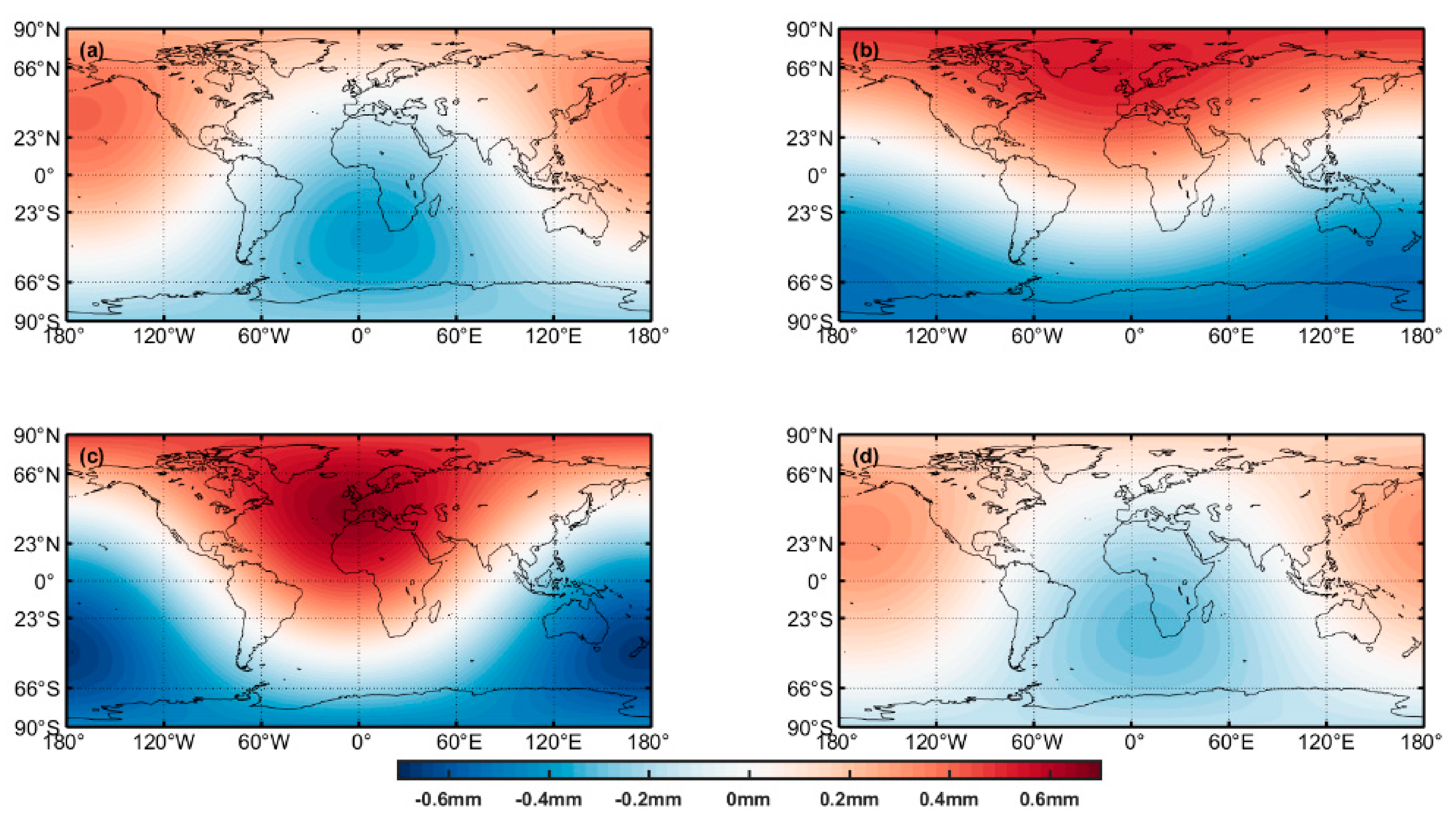
By using the derived degree-1 Stokes coefficients (please refer to Appendix A for more details) and degree > 1 Stokes coefficients of the LDCmgm90 dataset, we derive the corresponding horizontal and radial loading deformation separately after removing GIA effects. Obvious annual fluctuation is observed in degree-1 radial loading deformation in 2010 (Figure 2), which is similar in other years.
Global distribution of degree > 1 loading deformation is significantly more complex due to the contributions of time-dependent precipitation, discharge of hydrology and atmospheric and oceanic mass redistribution.
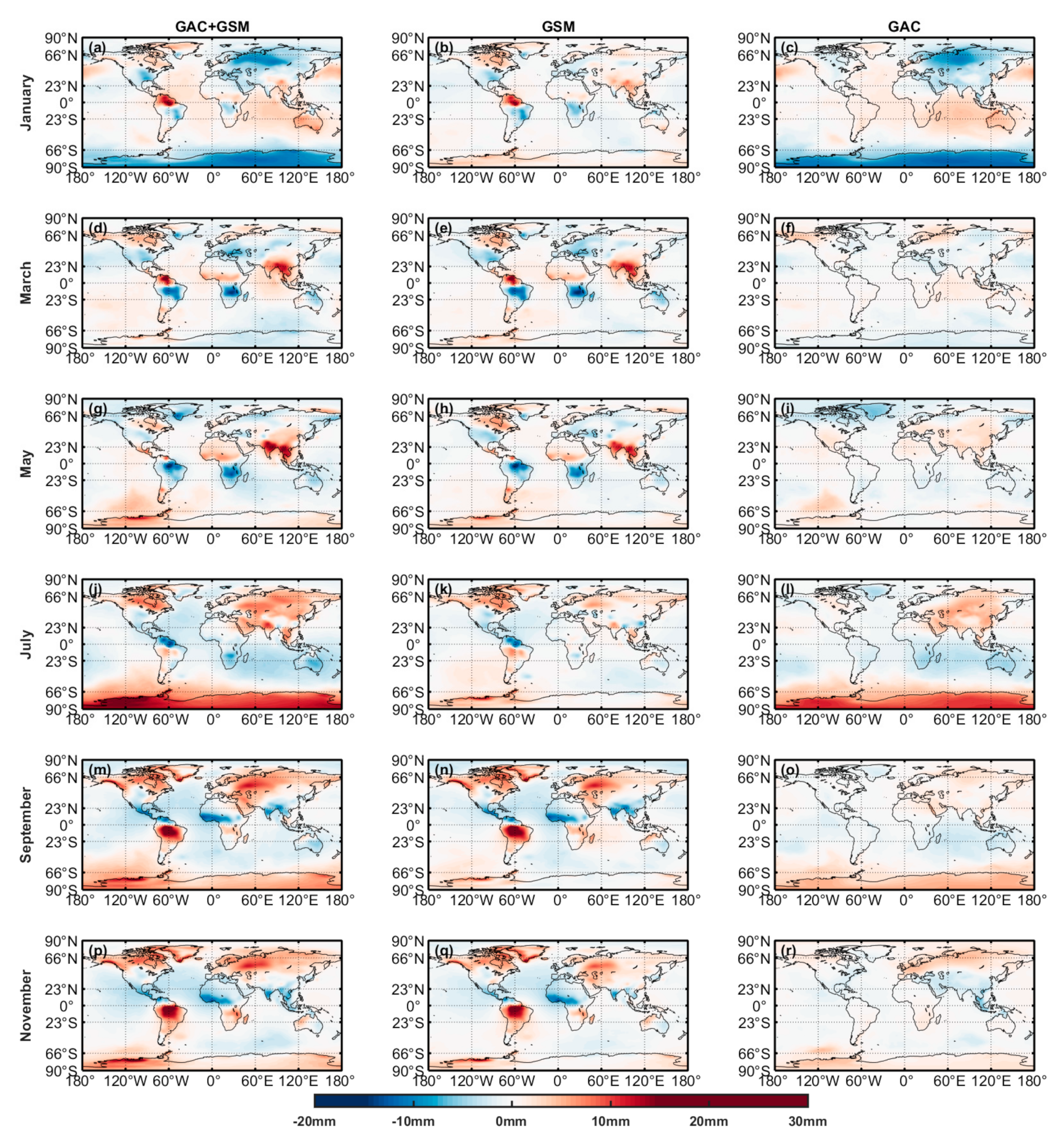
Radial loading deformation is significantly larger than horizontal loading deformation. Globally, in 2010, absolute values of radial loading deformation in middle and northern high latitudes remain less than 15 mm, while Antarctica and the tropical continents of South America, central Africa, southern Asia and northern Australia have significant annual loading deformation variations with amplitudes larger than 15 mm (see Figure 3, line 1, GAC + GSM).
To separate the contributions of different sources, we derive the global radial loading deformation of LDCmgm90 GSM and GAC products separately. We find that continental anomalies along the equator are only observed in GSM loading deformation (Figure 3, Line 2, GSM). These prominent annual variations reflect the changes of terrestrial water storage in tropical continents of both hemispheres since precipitation brings a large amount of water in their respective rainy seasons, leading to downward loading deformation, while high temperature and drought during dry seasons vaporize water, leading to upward loading deformation. In middle- and high-latitude areas, annual variations of GSM loading deformation are not so obvious due to less precipitation and lower temperature compared with the tropical area. Seasonal melting and freezing in high latitudes also contribute a little to GSM loading deformation, among which the Greenland coastline is the most prominent. However, annual loading deformation variations in middle and high latitudes are mainly caused by changes in atmospheric pressure and ocean bottom pressure, especially in Antarctica.
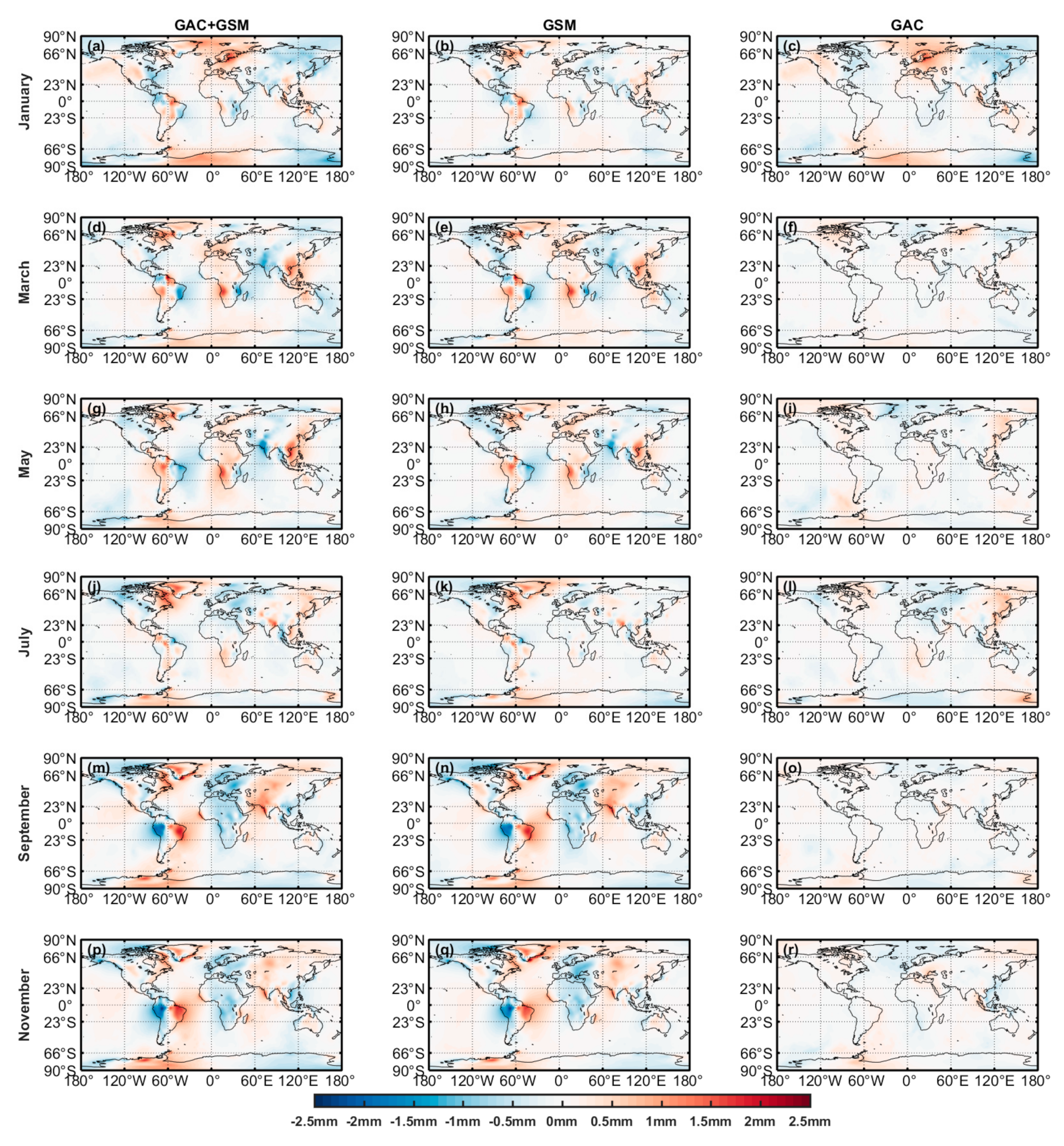
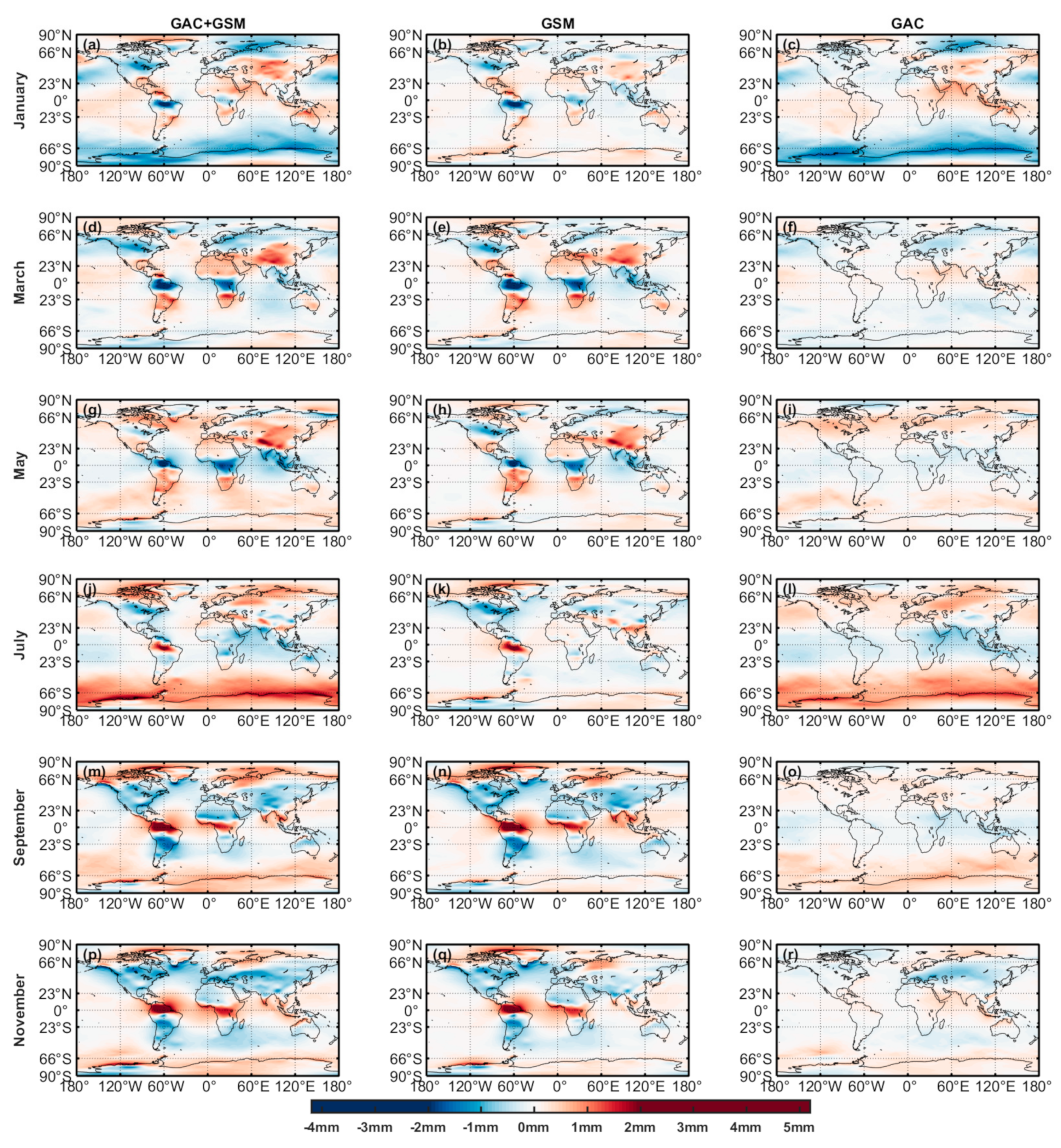
Periodical variation of horizontal loading deformation also supports our inferences for the vertical component. Besides, due to the property of Equation (3), latitudinal and longitudinal dipole-like horizontal anomalies form near the center of radial anomalies. Eastward and northward loading deformations always appear on the east and the north of a positive radial loading deformation and on the west and the south of a negative radial loading deformation (Figure 4 and Figure 5). On the whole, loading deformation diverges from a positive anomaly and converges to a negative anomaly. The direction of horizontal loading deformation is the same as the gradient of the vertical loading deformation field.

4. Discussion

We applied our LDCmgm90 GAC- and GSM-derived loading products to 249 IGb14 GPS time series processed by NGL to correct nontidal loading effects. Likewise, EOST and ESMGFZ atmospheric, oceanic and hydrological loading products were applied for comparison. Since these stations are scattered globally with diverse data characteristics and qualities, the results of loading corrections will reflect the reliability of load deformation models adopted. We also selected 12 of 249 GPS stations as examples, in which IMLS loading products were also applied.

4.1. Comparison of Annual Residual

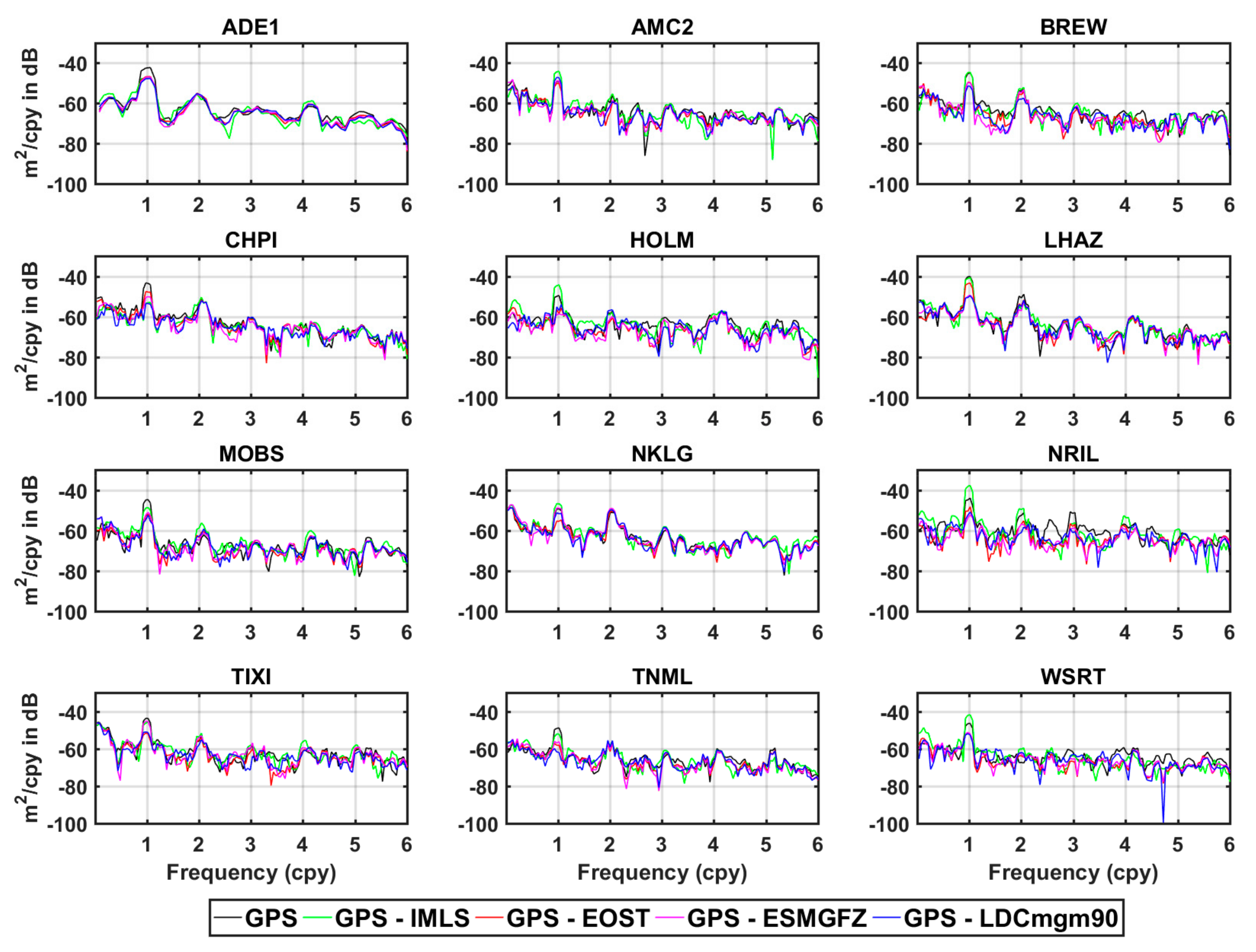
The up-component displacements of 12 IGb14 GPS stations are compared in Figure 6, in which loading effects have been removed by the four different loading products mentioned above (only in Figure 6 the trends are removed for easier comparisons of the seasonal signals). In most cases in the time domain, according to the remaining residuals, we find that more loading effects are removed by EOST, ESMGFZ and LDCmgm90 loadings compared with IMLS loading, especially at NRIL and WSRT. According to the corresponding residuals’ power spectrum density (PSD) shown in Figure 7 and annual amplitudes of time series listed in Table 2, we find that, among these 12 stations, significantly more annual loading is removed by LDCmgm90 datasets at 6 stations: ADE1, BREW, CHPI, MOBS, TNML and WSRT. The EOST loading is better at three stations: AMC2, NKLG and TIXI. ESMGFZ loading is better at three stations: HOLM, LHAZ and NRIL. No advantage of IMLS loading is found among these stations. In fact, applying IMLS loading often increases the annual amplitudes of the 12 residuals.
We also notice that at several stations, applying loading corrections leads to excess annual amplitudes instead of attenuating them, which indicates that worse results are induced by loading models. According to Table 2, compared with original GPS time series, annual loading amplitudes are successfully reduced at 6 stations with IMLS loading applied, at all 12 stations with EOST loading applied, at 10 stations with ESMGFZ loading applied and at 11 stations with LDCmgm90 loading models applied. Numerically, among these 12 stations, the most prominent improvement is brought by ESMGFZ loading at HOLM, where 91% up-component annual fluctuation in the original GPS signal is removed (only 0.21 mm remains).
The accuracy of hydrological loading is not as reliable as that of atmospheric and oceanic loadings due to the uneven distribution of continent water storage and much less accurate monitoring generally. Different hydrological models diverge from each other and may enlarge the residuals instead of attenuating them further. In Table 2, we notice that at eight stations (ADE1, AMC2, HOLM, MOBS, NKLG, NRIL, TIXI and WSRT), applying IMLS hydrological loading leads to larger annual residuals than applying IMLS atmospheric and oceanic loadings only, which is significantly improved by EOST, ESMGFZ and LDCmgm90 loading corrections. Therefore, we infer that EOST, ESMGFZ and LDCmgm90 models contain better hydrological loading information compared with IMLS loading.
Divergences between different loading models are smaller in other frequency bands at these 12 stations (such as semiannual loading, see frequency = 2 cpy in Figure 7 and Table 3). However, since loading effects are mainly annual fluctuations [5,8], discrepancies among loading models are mainly introduced by their annual signals, which should represent the quality of loading models. Therefore, due to the smaller time- and frequency-domain annual residual and better hydrological loading information involved, we believe that EOST, ESMGFZ and LDCmgm90 loadings are generally better than IMLS loading.

4.2. Loading Due to Seasonal Mass Redistributions

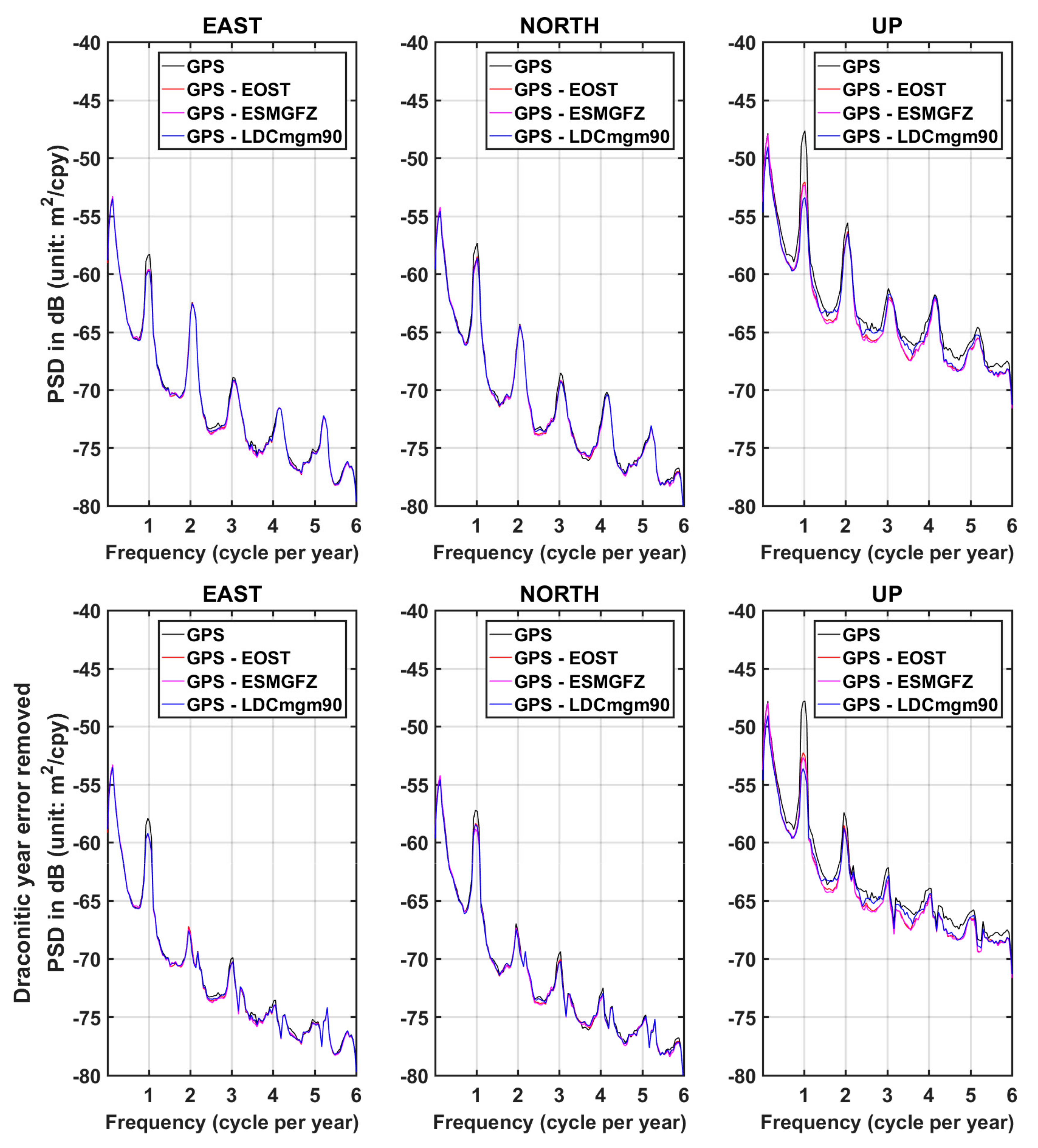
We removed the means and trends of all the relevant data in order to estimate the improvement of seasonal loading correction brought by our LDCmgm90 loading models compared with EOST and ESMGFZ datasets. First of all, we calculated the mean PSD of 249 IGb14 GPS time series with different loading correction models applied (see Figure 8). One can see the LDCmgm90 is the most efficient in attenuating the annual signal in GPS data, especially in the up-component. Besides, long-period variations of up-component GPS time series are also improved by LDCmgm90 compared with EOST and ESMGFZ. However, there are also strong peaks of draconitic year error (with period 351.2 day or frequency 1.04 cpy; also see Ray et al. [3]) and its higher harmonics (peaks near the 2, 3, 4 and 5 cpy) as shown by Figure 8. These draconitic year errors in GPS data have nothing to do with loading but also contribute greatly to the scatter of GPS position residual, which can be well corrected by least-square fitting (see three bottom subplots in Figure 8). On the other hand, both the EOST and ESMGFZ have better performances than LDCmgm90 for up-component variations between draconitic peaks, the cause of which is not quite certain but could be a limitation of the frequency and spatial resolutions (~6 cpy and ~2 degrees, respectively) of the LDCmgm90 data (it is rather common that there is no data point at the frequency of interest and thus the plots are impacted by its neighboring frequency points, due to the limited frequency domain sampling rate caused by the finite length of the time series of interest).
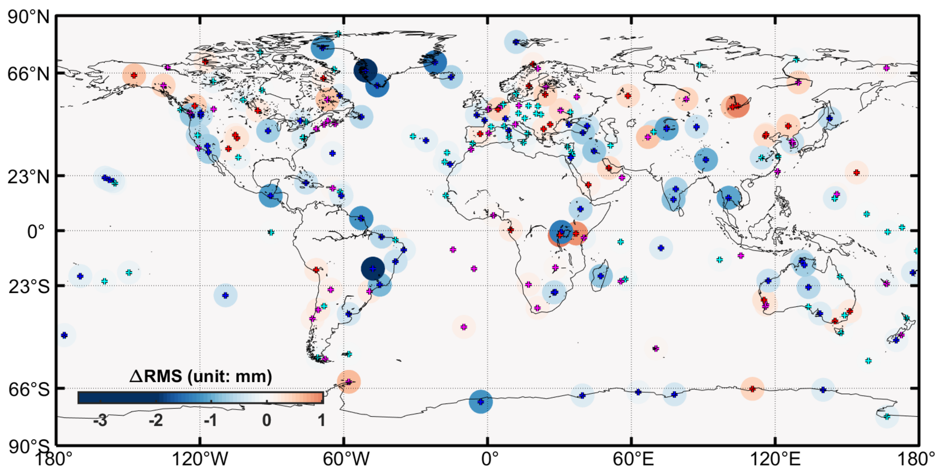
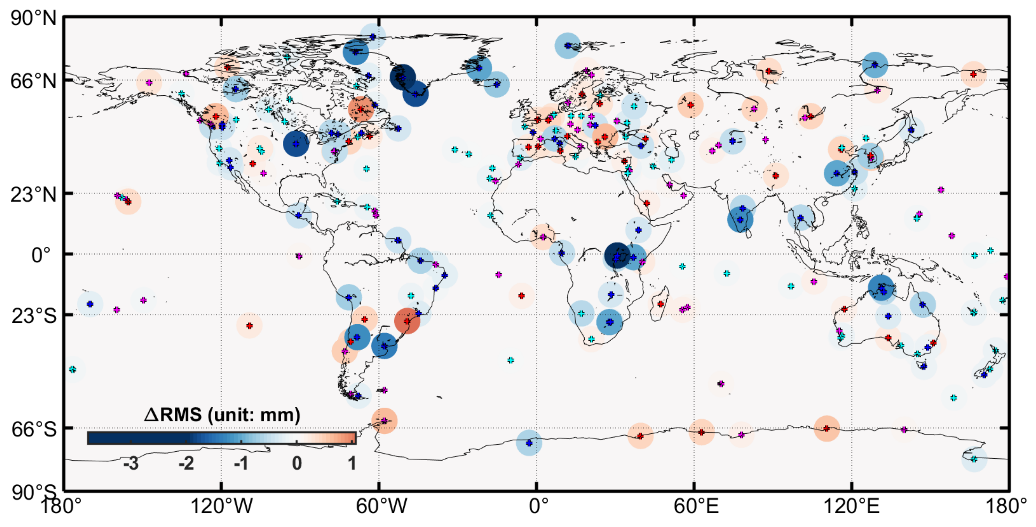
Root mean square (RMS) of detrended GPS residual is a vital index to estimate the quality of a loading model (the mean value of each time series is removed before time-domain analyses). Globally, compared with applying EOST and ESMGFZ loadings, applying LDCmgm90 loading improves the residual RMS at more of the 249 IGb14 GPS stations involved in this research. Up-component RMS variation (ΔRMS) brought by LDCmgm90 loading compared with applying either EOST loading or ESMGFZ loading is shown in Figure 9 and Figure 10, respectively. Besides, statistical information about RMS improvement ratio is listed in Table 4 and Table 5.
Compared with original GPS signal (Table 4), applying LDCmgm90 loading successfully reduces up-component RMS at 218 (equaling 87.55%) GPS stations, which is slightly more than applying EOST or ESMGFZ loading. When significantly improved (RMS improvement ratio > 5%) stations are considered only, LDCmgm90 loading is about 4% better than EOST and matches ESMGFZ loading.
In horizontal components, LDCmgm90 roughly matches EOST and ESMGFZ; differences between RMS with either loading model applied at most stations are within 5%. Numerically, according to Table 5, applying LDCmgm90 loading models instead of EOST loading models reduces 128 (equaling 51.41%) stations’ east-component RMS and 136 (equaling 54.62%) stations’ north-component RMS, which is slightly better when compared with ESMGFZ, in which 122 (equaling 49.00%) stations’ east-component RMS and 115 (equaling 46.18%) stations’ north-component RMS are reduced by applying LDCmgm90.
However, as for the up-component loading, where signals are larger than the horizontal-component loading, applying LDCmgm90 loading significantly decreases residuals’ RMS at 155 (equaling 62.25%) globally distributed GPS stations compared with applying EOST loading models, among which improvements at 81 (equaling 32.53%) stations are larger than 5%. Compared with ESMGFZ loading, applying LDCmgm90 loading also reduces 142 (equaling 57.03%) stations’ up-component residuals’ RMS, among which improvements at 72 (equaling 28.92%) stations are larger than 5%. The most obvious RMS improvements are found in high-latitude regions of the northern hemisphere, especially at stations located along Greenland’s coastline. The largest RMS decrease is found at KELY (66.987°N, 50.945°W; vs. EOST: −3.40 mm; vs. ESMGFZ: −3.78 mm), while the largest RMS increases are found at NURK (1.945°S, 30.09°S; vs. EOST: −1.02 mm) and UFPR (25.448°S, 49.231°W; vs. ESMGFZ: −1.07 mm). We infer that the better annual and long-period signals contribute to the up-component superiority of LDCmgm90 compared to EOST and ESMGFZ.
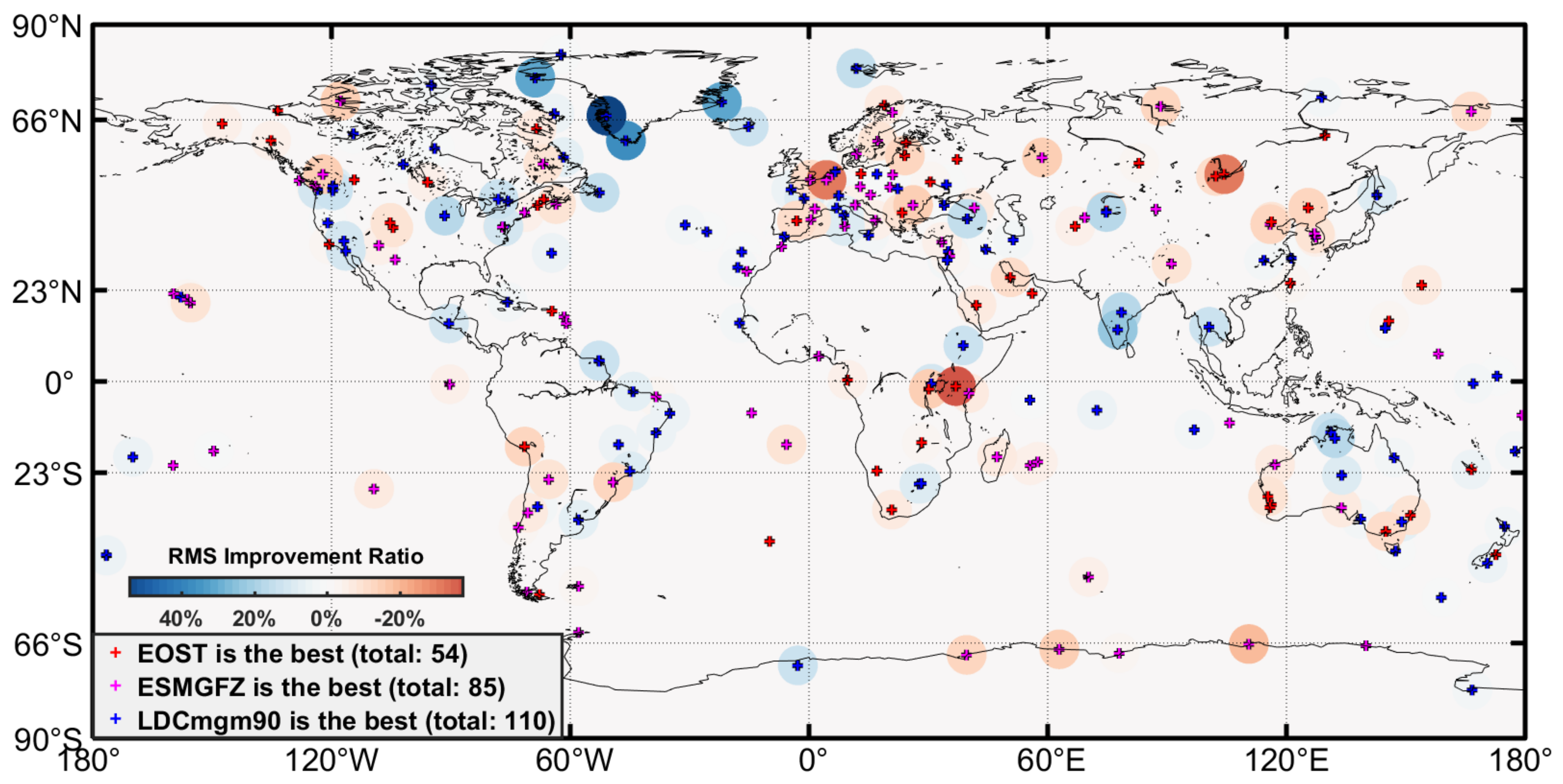
To better understand these three loading models, we also compared EOST, ESMGFZ and LDCmgm90 together, finding the best loading model for each station involved in this research and calculating the RMS improvement ratio of GPS residuals brought by LDCmgm90 compared with the better result of applying EOST and ESMGFZ loadings (Figure 11). To reach the smallest RMS of GPS residuals, applying EOST is the best choice for 54 (21.69%) stations, applying ESMGFZ is the best choice for 85 (34.14%) stations and applying LDCmgm90 is the best choice for 110 (44.18%) stations. Regionally, EOST-best stations lie mainly in the middle-latitude area of North America and Asia. ESMGFZ-best stations are mainly in western Europe. LDCmgm90-best stations are widely distributed around the world, especially along the coastline of Greenland.
Therefore, according to the comparison of 249 globally distributed IGb14 GPS stations, especially the improvement in removing up-component effects, we conclude that LDCmgm90 loading is reliable and generally better than EOST loading and ESMGFZ loading.

4.3. Contributions of Secular or Long-Term Mass Redistributions

Loading affects not only seasonal variations but also trends in GPS measurements, which should be appropriately considered by a complete loading model (note that many long-period geophysical signals, e.g., the ~18.6-year tide, may look like trends for the relatively short GPS time series; thus, “trends” here may contain contributions from these long-period geophysical signals). Therefore, to test the secular or long-term signals of LDCmgm90 loading, we only removed the means but retained the trends of all data, and we applied GIA corrections (ICE6Gavg-GPS model) to GPS data and LDCmgm90 loading (termed “trend-retained” for short hereafter). The analyses are similar to those in Section 4.2. Comparisons are listed in Table 6 and Table 7.
According to the comparison of 249 GPS stations in Table 6, when trends are considered, the number of stations significantly improved (RMS improvement ratio > 5%) by applying EOST and ESMGFZ loadings decreases by 15~20%, while the number of stations significantly improved by applying LDCmgm90 loading varies only 2%, which is 16% better than EOST loading and 18% better than ESMGFZ loading.
Applying LDCmgm90 loading successfully reduces up-component RMS at 201 (equaling 80.72%) GPS stations, which is similar to applying EOST loading and 12% more than applying ESMGFZ loading. On the other hand, the ~14% larger improvement of the EOST model with respect to the ESMGFZ model is not found in trend-removed comparison. This may be due to the facts that the former adopts the ECMWF reanalysis (ERA5) of atmospheric data and the associated oceanic and hydrological models are forced by both surface pressure and winds (more practical), which induces better trend signals, while the ESMGFZ only uses ECMWF operational data and its associated ocean model is forced only by surface pressure (less practical; operational data usually have poorer quality than reanalysis data).
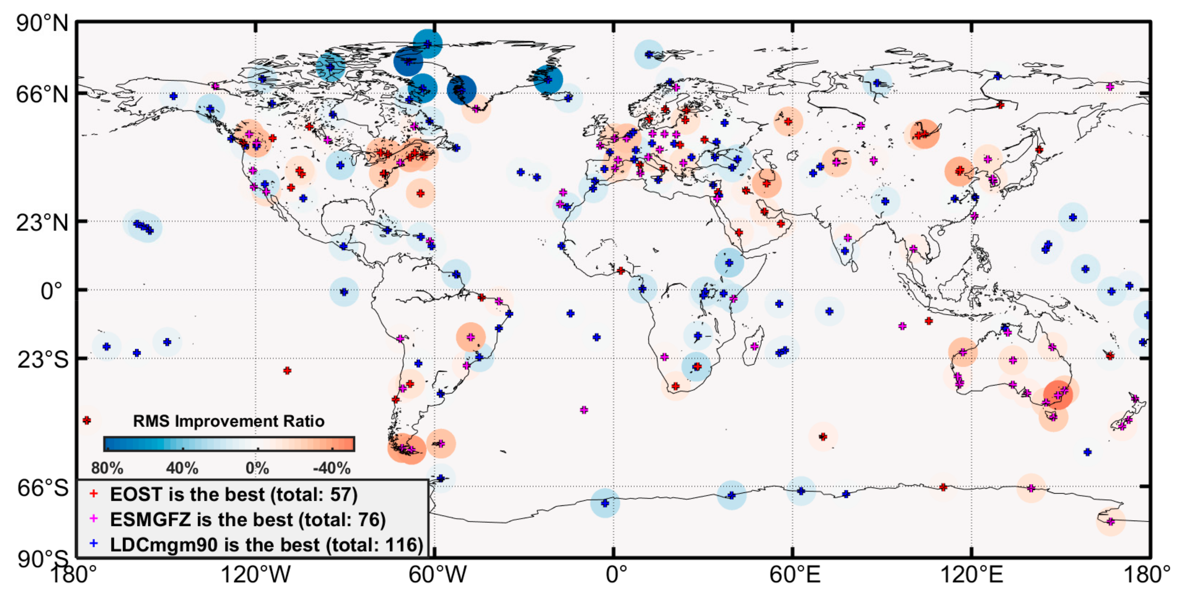
Improvement brought by the trend of LDCmgm90 loading can also be observed in Table 7, where significantly improved (RMS improvement ratio > 5%) stations rise 11% and 15% when compared with EOST and ESMGFZ results, respectively. Total numbers of improved stations also slightly increase. We also repeat the three-model comparison similar to Figure 11, the result of which is given in Figure 12. We find that the largest RMS improvement ratio is about 80%, which is nearly double that in Figure 11. Besides, when trends are considered, applying LDCmgm90 is the best choice for 116 (46.59%) stations, slightly more than trend-removed condition.
In order to show the advantages of long-term and annual signals in LDCmgm90 loading more clearly, we calculate the improvement of LDCmgm90 loading in long-term (with periods > 5 years) and annual frequency bands (with periods between 338 and 410 days) compared with EOST and ESMGFZ loadings (Table 8). We find that 49% EOST and 49.8% ESMGFZ long-term residuals and 57.83% EOST and 55.02% ESMGFZ annual residuals are significantly improved, larger than 43.37% and 44.58% in Table 7 where all <6 cpy signals (period > 2 months) are considered, supporting the contributions of LDCmgm90 loading in long-term and annual bands. In the meanwhile, total numbers of improved stations in Table 8 remain similar compared with Table 7, indicating that (1) general advantages of LDCmgm90 loading still exist and (2) EOST and ESMGFZ loading models also perform well in other seasonal variations, which corresponds with PSD shown in Figure 8.
Therefore, according to the trend-retained comparison in this section and band comparison in Table 8, we confirm that not only seasonal variations but also long-term signals in LDCmgm90 loading are better than those in EOST and ESMGFZ loadings.

5. Conclusions

By using LDCmgm90 multiple-data-based monthly gravity dataset and estimating its degree-1 Stokes coefficients, we have obtained the complete LDCmgm90 atmospheric, oceanic and hydrological loading models. Globally, we compared LDCmgm90 loading model with GCM-based loading models provided by the EOST Loading Service and ESMGFZ by applying them to 249 globally distributed IGb14 GPS stations processed by NGL to remove their loading effects. Loading models provided by IMLS were also applied to 12 GPS stations.
Our research shows that the LDCmgm90 loading model can reliably remove loading effects in GPS time series and is likely to achieve similar or even better results compared with other latest loading models. In general, according to our numerical results, we infer that the EOST and ESMGFZ loading models are better than the IMLS loading, but the LDCmgm90 loading is even better, not only for GPS sites on the continents but also for those on the islands surrounded by the oceans. The better annual, trend and long-period information, especially that of continent water, contribute to the superiority of LDCmgm90 loading compared with other loading products and therefore lead to significant improvements in the LDCmgm90 model with respect to the EOST and ESMGFZ models.
When all the data trends are removed, applying LDCmgm90 loading successfully attenuates up-component loading effects at 218 (87.55%) GPS stations. In addition, time- and frequency-domain analyses show that LDCmgm90 has better performance than EOST at 155 (62.25%) GPS stations and ESMGFZ at 142 (57.03%) GPS stations. These values increase to 160 (64.26%) for EOST and 152 (61.04%) for ESMGFZ if all the data trends are retained, implying that LDCmgm90 can provide better secular or long-term global mass redistributions. Therefore, the LDCmgm90 loading model is the best choice to remove not only seasonal but also secular or long-term loading signals in GPS site displacement data, providing a chance to explore other geophysical causes buried in the residual secular or long-term signals in the GPS data. The LDCmgm90 loading model is available upon request.
It should be mentioned that there are also some limitations in the LDCmgm90 loading model, such as limited spatial (~2-degree) and frequency (~6-cpy) resolutions and availability limited to the GRACE mission period (~2002–2017, but the LDCmgm90 will be extended to include the GRACE Follow-On data in the future). While the ~6-cpy frequency resolution should be enough for global mass loading, the ~2-degree spatial resolution could be insufficient for some small regions with large local hydrological signals, such as California. Thus, no load model is perfect; each contains certain defects and even errors. Users should beware of applying load corrections to GPS time series data blindly assuming that no new errors will be introduced.

Author Contributions

Conceptualization, J.R., J.L. (Jiancheng Li) and W.C.; methodology, J.R., W.C. and T.v.D.; software, J.L. (Jiesi Luo); validation, J.R. and W.C.; formal analysis, J.L. (Jiesi Luo); investigation, J.L. (Jiesi Luo); resources, J.L. (Jiesi Luo); data curation, J.L. (Jiesi Luo) and W.C.; writing—original draft preparation, J.L. (Jiesi Luo) and W.C.; writing—review and editing, J.R., W.C. and T.v.D.; visualization, J.L. (Jiesi Luo); supervision, J.L. (Jiancheng Li); project administration, W.C.; funding acquisition, W.C. All authors have read and agreed to the published version of the manuscript.

Funding

This research was funded by the National Natural Science Foundation of China, grant numbers 41874025 and 41474022. The APC was funded by the National Natural Science Foundation of China, grant number 41874025.

Institutional Review Board Statement

Not applicable.

Informed Consent Statement

Not applicable.

Data Availability Statement

The EOST, ESMGFZ and IMLS loading data are respectively available at http://massloading.net/, http://loading.u-strasbg.fr/index.php and http://rz-vm115.gfz-potsdam.de:8080/repository (accessed on 20 September 2021). The LDCmgm90 model is available at https://doi.org/10.6084/m9.figshare.7874384.v4 (accessed on 20 September 2021). The LDCmgm90 loading model is available upon request to W.C. and J.L. (Jiesi Luo).

Acknowledgments

We thank the EOST, ESMGFZ and IMLS teams for making their loading models publicly available.

Conflicts of Interest

The authors declare no conflict of interest.

Appendix A. Estimations of Degree-1 Stokes Coefficients and Geocenter Variation of LDCmgm90
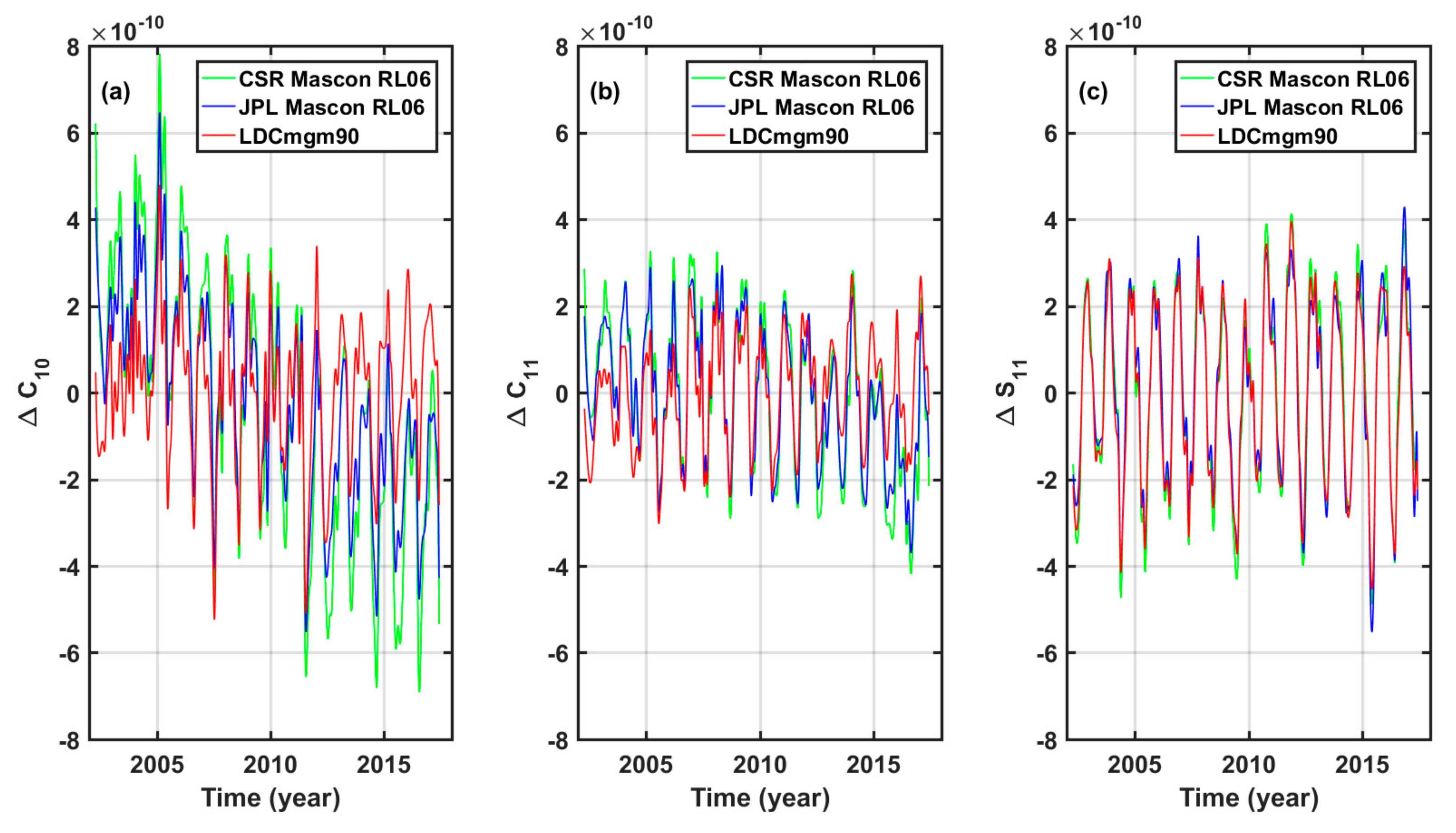
We estimate the LDCmgm90 degree-1 Stokes coefficients ( Δ C 10 L D C m g m 90 , Δ C 11 L D C m g m 90 and Δ S 11 L D C m g m 90 ) and compare them with degree-1 coefficients of CSR and JPL RL06 GRACE Mascon solutions (Figure A1). To recover the corresponding total global effects of the original Mascon solution, we remove GAD products, reconsider the ICE-6G-D model and restore GAC products (total Mascon = original Mascon product—GAD + GIA + GAC). Our results, especially ΔS11, have good agreement with other degree-1 coefficients.
Figure A1. Time series of fully normalized degree-1 Stokes coefficients of CSR Mascon RL06 solutions (green line), JPL Mascon RL06 solution (blue line) and LDCmgm90 (red line) derived in this research according to Swenson et al. [49] spanning 04/2002~06/2017. (a) ΔC10; (b) ΔC11; (c) ΔS11. Please notice that GAC and GIA are included in this figure.
Remotesensing 13 04408 g0a1
The annual amplitudes and phases of LDCmgm90 degree-1 Stokes coefficients are compared with values from RL06 Mascon solutions from CSR and JPL in Table A1. Y-component annual fluctuation of LDCmgm90 total geocenter variation has good agreement with CSR and JPL Mascon solutions. However, phases of X- and Z-components of LDCmgm90 total geocenter variation are slightly larger than others. Our X-component trend also deviates from CSR and JPL Mascon solutions, while X-component and Z-component are similar to CSR and JPL Mascon solutions separately.
Table A1. Annual amplitudes, annual phase and linear trends of total geocenter variation of 04/2002~06/2017. CSR and JPL Mascon RL06 solutions are given as reference 1.
ModelXσX YσYZσZ
Annual Amplitude (unit: mm)
CSR Mascon2.060.023.060.022.840.02
JPL Mascon1.820.022.880.021.910.02
LDCmgm901.520.012.930.011.910.02
Annual Phase (unit: day) 2
CSR Mascon33.880.48179.560.3034.470.42
JPL Mascon39.480.49179.750.3138.700.57
LDCmgm9058.950.50179.700.2674.570.58
Linear Trend (unit: mm/year)
CSR Mascon−0.070.05−0.460.051.010.06
JPL Mascon−0.050.040.030.040.580.05
LDCmgm900.130.04−0.370.040.620.06
1 Values in this table are derived by least-square fitting, with σ as the formal errors of fitting. 2 Annual phases are defined by using sine function. Please notice that to describe the phase shift of the annual signal in its period, the unit of the annual phase is converted from radians to days by multiplying 365.25/2π.

Appendix B. Sources of GPS Measurement Errors and Other Systematic Effects

Ray [1] listed many sources of measurement error and other systematic effects, such as draconitic errors, local site errors, temperature cycle errors and errors in IERS models. In this appendix, sources of annual errors are summarized briefly:
  • Draconitic Year Errors
Draconitic year signal (period = 351.2 days) has strong spatial correlations in IGS position time series [3,4].
  • Temperature Cycle
Thermal cycle of the Earth will cause expansions of antenna structure and surrounding bedrock [13].
  • Errors in IERS Models
The recommended IERS Conventions (2010) models suffer weaknesses in various respects, including deficiencies and errors in some models as well as a lack of any standard model for some effects. Models with known errors include ocean tidal loading [16], diurnal and semidiurnal EOP tides that cause aliases into longer-period signals [53] though an alternative model has been put forward outside the formal conventions (https://ivscc.gsfc.nasa.gov/hfeop_wg/, accessed on 27 October 2021), possible lateral heterogeneity effects in the solid Earth tidal displacement [54] and the atmospheric pressure loading (e.g., S1, S2). Time variation of the low-degree geopotential terms has been recognized, but no standard model is recommended for all techniques. In fact, there have been no major updates to any IERS models in recent years apart from the return to a secular mean pole model in 2018 that replaced the ill-considered quadratic model recommended for several years. As a consequence, the techniques and analysis centers have adopted divergent approaches in some cases.
  • Antenna-Related Effects
Local multipath errors and antenna calibration errors may add aliasing signals to observation records. Snow, ice cover and rain may also affect antennas by adding annual signals or changing sky visibility, especially in high latitudes [4]:
  • Receiver Hardware Change [4]
  • Troposphere Delay Mismodeling (see for example Martens et al. [41])
  • Aliasing in Long-Term Time Series Stacking [4]
  • Processing Differences among Analysis Centers (ACs)
  • Clear differences between products for the same stations released by ACs sometimes exist [4].

References

  1. Ray, J. Precision and Accuracy of GNSS Positions; Lecture Presented at School of Geodesy and Geomatics; Wuhan University: Wuhan, China, 4 January 2015. [Google Scholar]
  2. Petit, G.; Luzum, B. IERS Conventions (2010), IERS Technical Notes 36; Verlag des Bundesamts für Kartographie und Geodäsie: Frankfurt, Germany, 2010; p. 179. ISBN 3-89888-989-6. [Google Scholar]
  3. Ray, J.; Altamimi, Z.; Collilieux, X.; van Dam, T. Anomalous harmonics in the spectra of GPS position estimates. GPS Solut. 2008, 12, 55–64. [Google Scholar] [CrossRef]
  4. Ray, J.; Rebischung, P.; Griffiths, J. IGS polar motion measurement accuracy. Geod. Geodyn. 2017, 8, 413–420. [Google Scholar] [CrossRef]
  5. van Dam, T.; Wahr, J.; Milly, P.; Shmakin, A.; Blewitt, G.; Lavallee, D.; Larson, K.M. Crustal displacements due to continental water loading. Geophys. Res. Lett. 2001, 28, 651–654. [Google Scholar] [CrossRef] [Green Version]
  6. Van Dam, T.; Collilieux, X.; Wuite, J.; Altamimi, Z.; Ray, J. Nontidal ocean loading: Amplitudes and potential effects in GPS height time series. J. Geodyn. 2012, 86, 1043–1057. [Google Scholar] [CrossRef] [Green Version]
  7. Blewitt, G.; Lavallee, D.; Clarke, P.; Nurutdinov, K. A newglobal mode of Earth deformation: Seasonal cycle detected. Science 2001, 294, 2342–2345. [Google Scholar] [CrossRef] [Green Version]
  8. Dong, D.; Fang, P.; Bock, Y.; Cheng, M.; Miyazaki, S. Anatomy of apparent seasonal variations from GPS-derived site position time series. J. Geophys. Res. 2002, 107, 2075. [Google Scholar] [CrossRef] [Green Version]
  9. Kaniuth, K.; Vetter, S. Estimating atmospheric pressure loading regression coefficients from GPS observations. GPS Solut. 2006, 10, 126–134. [Google Scholar] [CrossRef]
  10. Grapenthin, R.; Sigmundsson, F.; Geirsson, H.; Árnadóttir, T.; Pinel, V. Icelandic rhythmic: Annual modulation of land elevation and plate spreading by snow load. Geophys. Res. Lett. 2006, 33, L24305. [Google Scholar] [CrossRef] [Green Version]
  11. Tregoning, P.; Watson, C. Atmospheric effects and spurious signals in GPS analyses. J. Geophys. Res. 2009, 114, B09403. [Google Scholar] [CrossRef] [Green Version]
  12. King, M.A.; Watson, C.S.; Penna, N.T.; Clarke, P.J. Subdailysignals in GPS observations and their effect at semiannual and annual periods. Geophys. Res. Lett. 2008, 35, L03302. [Google Scholar] [CrossRef] [Green Version]
  13. Yan, H.; Chen, W.; Zhu, Y.; Zhang, W.; Zhong, M. Contributions of thermal expansion of monuments and nearby bedrock to observed GPS height changes. Geophys. Res. Lett. 2009, 36, L13301. [Google Scholar] [CrossRef] [Green Version]
  14. Jiang, Y.; Dixon, T.; Wdowinski, S. Accelerating uplift in the north Atlantic region as an indicator of ice loss. Nat. Geosci. 2010, 3, 404–407. [Google Scholar] [CrossRef]
  15. Matsuo, K.; Heki, K. Time-variable ice loss in Asian high mountains from satellite gravimetry. Earth Planet. Sci. Lett. 2010, 290, 30–36. [Google Scholar] [CrossRef]
  16. Yuan, L.G.; Chao, B.F. Analysis of tidal signals in surface displacement measured by a dense continuous GPS array. Earth Planet. Sci. Lett. 2012, 355–356, 255–261. [Google Scholar] [CrossRef]
  17. van Dam, T.; Wahr, J. Displacement of the Earth’s surface due to atmospheric loading: Effects on gravity and baseline measurements. J. Geophys. Res. 1987, 92, 1282–1286. [Google Scholar] [CrossRef]
  18. Mangiarotti, S.; Cazenave, A. Annual vertical crustal motions predicted from surface mass redistribution and observed by space geodesy. J. Geophys. Res. 2001, 106, 4277–4291. [Google Scholar] [CrossRef]
  19. Blewitt, G. Self-consistency in the reference frames, geocenter definition and surface loading of the solid earth. J. Geophys. Res. 2003, 108, 2103. [Google Scholar] [CrossRef] [Green Version]
  20. Chen, W.; Ray, J.; Shen, W.B.; Huang, C.L. Polar motion excitations for an Earth model with frequency-dependent responses: 2 Numerical tests of the meteorological excitations. J. Geophys. Res. Solid Earth 2013, 118, 4995–5007. [Google Scholar] [CrossRef]
  21. Chen, W.; Li, J.C.; Ray, J.; Cheng, M.K. Improved geophysical excitations constrained by polar motion observations and GRACE/SLR time-dependent gravity. Geod. Geodyn. 2017, 6, 11–22. [Google Scholar] [CrossRef]
  22. Taplay, B.D.; Bettadpur, S.; Ries, J.C.; Thompson, P.F.; Watkins, M.M. GRACE measurements of mass variability in the Earth system. Science 2004, 305, 503–505. [Google Scholar] [CrossRef] [Green Version]
  23. Davis, J.; Elósegui, P.; Mitrovica, J.; Tamisiea, M. Climate-driven deformation of the solid Earth from GRACE and GPS. Geophys. Res. Lett. 2004, 31, L24605. [Google Scholar] [CrossRef] [Green Version]
  24. Yan, H.; Chen, W.; Yuan, L. Crustal vertical deformation response to different spatial scales of GRACE and GCMs surface loading. Geophys. J. Int. 2016, 204, 505–516. [Google Scholar] [CrossRef] [Green Version]
  25. Fu, Y.; Freymueller, J.T. Seasonal and long-term vertical deformation in Nepal Himalaya constrained by GPS and GRACE measurements. J. Geophys. Res. 2012, 117, B03407. [Google Scholar] [CrossRef]
  26. Chanard, K.; Fleitout, L.; Calais, E.; Rebischung, P.; Avouac, J.-P. Toward a global horizontal and vertical elastic load deformation model derived from GRACE and GNSS station position time series. J. Geophys. Res. Solid Earth 2018, 123, 3225–3237. [Google Scholar] [CrossRef]
  27. Wahr, J.; Molenaar, M.; Bryan, F. Time variability of the earth’s gravity field: Hydrological and oceanic effects and their possible detection using grace. J. Geophys. Res. Solid Earth 1998, 103, 30205–30229. [Google Scholar] [CrossRef]
  28. Chen, J.L.; Wilson, C.R.; Famiglietti, J.S.; Rodell, M. Spatial sensitivity of GRACE time-variable gravity observations. J. Geophys. Res. 2005, 110, B08408. [Google Scholar]
  29. Chen, W.; Luo, J.; Ray, J.; Yu, N.; Li, J.C. Multiple-data-based monthly geopotential model set LDCmgm90. Sci. Data 2019, 6, 228. [Google Scholar] [CrossRef] [PubMed] [Green Version]
  30. Wu, X.; Heflin, M.B.; Ivins, E.R.; Fukumori, I. Seasonal and interannual global surface mass variations from multisatellite geodetic data. J. Geophys. Res. 2006, 111, B09401. [Google Scholar] [CrossRef] [Green Version]
  31. Cheng, M.K.; Ries, J.C.; Tapley, B.D. Variations of the Earth’s figure axis from satellite laser ranging and GRACE. J. Geophys. Res. 2011, 116, B01409. [Google Scholar] [CrossRef] [Green Version]
  32. Cheng, M.K.; Tapley, B.D.; Ries, J.C. Deceleration in the Earth’s oblateness. J. Geophys. Res. Solid Earth 2013, 118, 740–747. [Google Scholar] [CrossRef]
  33. Bar-Sever, Y.E. A new model for GPS yaw attitude. J. Geod. 1996, 70, 714–723. [Google Scholar] [CrossRef]
  34. Bar-Sever, Y.E.; Kuang, D. New Empirically-Derived Solar Radiation Pressure Model for GPS Satellites; Institute of Navigation: Portland, OR, USA, 2005; pp. 42–160. Available online: http://ipnpr.jpl.nasa.gov/progress_report/42-160/title.htm (accessed on 6 December 2020).
  35. Bassiri, S.; Hajj, G.A. Higher-order ionospheric effects on the global positioning systems observables and means of modeling them. Manuscr. Geodtica 1993, 18, 280–289. [Google Scholar]
  36. Bevis, M.; Businger, S.; Chiswell, S.; Herring, T.A.; Anthes, R.A.; Rocken, C.; Ware, R.H. GPS meteorology: Mapping zenith wet delays onto precipitable water. J. Appl. Meteorol. 1994, 33, 378–386. [Google Scholar] [CrossRef]
  37. Blewitt, G. An automatic editing algorithm for GPS data. Geophys. Res. Lett. 1990, 17, 199–202. [Google Scholar] [CrossRef] [Green Version]
  38. Kedar, S.; Hajj, G.; Wilson, B.; Heflin, M. The effect of the second order GPS ionospheric correction on receiver positions. Geophys. Res. Lett. 2003, 30, 1829. [Google Scholar] [CrossRef]
  39. Kreemer, C.; Blewitt, G.; Klein, E. A geodetic plate motion and Global Strain Rate Model. Geochem. Geophys. Geosystems 2014, 15, 3849–3889. [Google Scholar] [CrossRef]
  40. Sibois, A.; Selle, C.; Desai, S.; Sibthorpe, A.; Weiss, J. GSPM13: An updated empirical model for solar radiation pressure forces acting on GPS satellites. In Proceedings of the IGS Workshop 2014, Pasadena, CA, USA, 23–27 June 2014. [Google Scholar]
  41. Martens, H.R.; Argus, D.F.; Norberg, C.; Blewitt, G.; Herring, T.A.; Moore, A.W.; Hammond, W.C.; Kreemer, C. Atmospheric pressure loading in GPS positions: Dependency on GPS processing methods and effect on assessment of seasonal deformation in the contiguous USA and Alaska. J. Geod. 2020, 94, 115. [Google Scholar] [CrossRef]
  42. Petrov, L.; Boy, J.-P. Study of the atmospheric pressure loading signal in VLBI observations. J. Geophys. Res. 2004, 109, B03405. [Google Scholar]
  43. Petrov, L. The International Mass loading Service. arXiv 2015, arXiv:1503.00191. [Google Scholar]
  44. Carrère, L.; Lyard, F. Modelling the barotropic response of the global ocean to atmospheric wind and pressure forcing—Comparisons with observations. Gephys. Res. Lett. 2003, 30, 1275–1278. [Google Scholar] [CrossRef] [Green Version]
  45. Rodell, M.; Houser, R.; Jambor, U.; Gottschalck, J.; Mitchell, K.; Meng, C.-J.; Arsenault, K.; Cosgrove, B.; Radakovich, J.; Bosilovich, M.; et al. The Global Land Data Assimilation System. Bull. Am. Meteorol. Soc. 2004, 85, 381–394. [Google Scholar] [CrossRef] [Green Version]
  46. Dill, R.; Dobslaw, H. Numerical simulations of global-scale high-resolution hydrological crustal deformations. J. Geophys. Res. Solid Earth 2013, 118, 5008–5017. [Google Scholar] [CrossRef]
  47. Dobslaw, H.; Bergmann-Wolf, I.; Dill, R.; Poropat, L.; Thomas, M.; Dahle, C.; Esselborn, S.; König, R.; Flechtner, F. A new high-resolution model of non-tidal atmosphere and ocean mass variability for de-aliasing of satellite gravity observations: AOD1B RL06. Geophys. J. Int. 2017, 211, 263–269. [Google Scholar] [CrossRef] [Green Version]
  48. Zhou, Y.; Yang, S.; Luo, J.; Ray, J.; Huang, Y.; Li, J. Global Glacial Isostatic Adjustment Constrained by GPS Measurements: Spherical Harmonic Analyses of Uplifts and Geopotential Variations. Remote Sens. 2020, 12, 1209. [Google Scholar] [CrossRef] [Green Version]
  49. Swenson, S.C.; Chambers, D.P.; Wahr, J. Estimating geocenter variations from a combination of GRACE and ocean model output. J. Geophys. Res. Solid Earth 2008, 113, B08410. [Google Scholar] [CrossRef] [Green Version]
  50. Han, D.; Wahr, J. The viscoelastic relaxation of a realistically stratified Earth, and a further analysis of post-glacial rebound. Geophys. J. Int. 1995, 120, 287–311. [Google Scholar] [CrossRef] [Green Version]
  51. Farrell, W.E. Deformation of the Earth by Surface loads. Rev. Geophys. Space Phys. 1972, 10, 761–797. [Google Scholar] [CrossRef]
  52. Chen, J.Y.; Pan, E.; Bevis, M. Accurate computation of the elastic load Love numbers to high spectral degree for a finely layered, transversely isotropic and self-gravitating Earth. Geophys. J. Int. 2018, 212, 827–838. [Google Scholar] [CrossRef]
  53. Griffiths, J.; Ray, J.R. Sub-daily alias and draconitic errors in the IGS orbits. GPS Solut. 2013, 17, 413–422. [Google Scholar] [CrossRef]
  54. Yuan, L.; Chao, B.F.; Ding, X.; Zhong, P. The tidal displacement field at Earth’s surface determined using global GPS observations. J. Geophys. Res. Solid Earth 2013, 118, 2618–2632. [Google Scholar] [CrossRef] [Green Version]
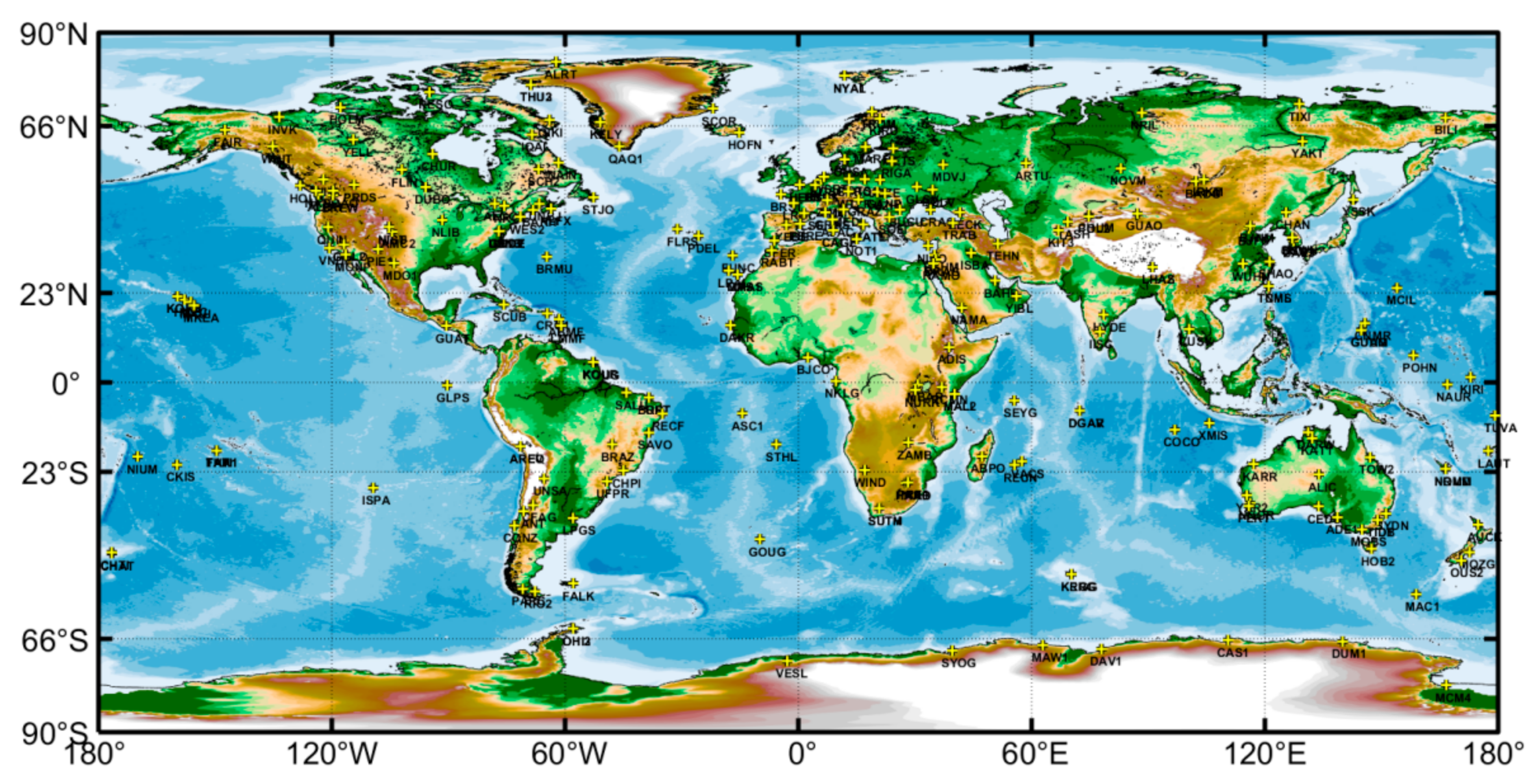
Figure 1. Distribution of 249 IGb14 GPS stations used in this research. Locations of these GPS stations are marked with yellow “+” with corresponding station name given below. Station names may overlap due to their dense distributions in several areas.
Remotesensing 13 04408 g001
Figure 2. Global distribution of degree-1 radial loading deformation of LDCmgm90 spherical harmonic solution. Four samples in 2010 are shown: (a) March, 2010; (b) June, 2010; (c) September, 2010; (d) December, 2010.
Remotesensing 13 04408 g002
Figure 3. Global distribution of degree >1 vertical loading deformation of LDCmgm90 spherical harmonic solutions in odd months of 2010. Different sources are shown in different columns: Column 1, GAC + GSM (a,d,g,j,m,p); Column 2, GSM (b,e,h,k,n,q); Column 3, GAC (c,f,i,l,o,r); In 2010, absolute values of loading deformation of the Earth seldom reach 15 mm except in several places such as the Amazon region, where about 28 mm at most appears. Therefore, the color representing radial loading deformation >15 mm or <−15 mm remains the same to reveal smaller details.
Remotesensing 13 04408 g003
Figure 4. Global distribution of degree >1 eastward loading deformation of LDCmgm90 spherical harmonic solutions in odd months of 2010. Different sources are shown in different columns: Column 1, GAC + GSM (a,d,g,j,m,p); Column 2, GSM (b,e,h,k,n,q); Column 3, GAC (c,f,i,l,o,r).
Remotesensing 13 04408 g004
Figure 5. Global distribution of degree >1 northward loading deformation of LDCmgm90 spherical harmonic solutions in odd months of 2010. Different sources are shown in different columns: Column 1, GAC + GSM (a,d,g,j,m,p); Column 2, GSM (b,e,h,k,n,q); Column 3, GAC (c,f,i,l,o,r); In 2010, only South America northward loading deformation >2 mm in several months, reaching 5.2 mm at most. Therefore, color representing northward loading deformation >2 mm or <−2 mm remains the same to reveal smaller details.
Remotesensing 13 04408 g005
Figure 6. Detrended up-component residuals of 12 IGb14 GPS stations in which IMLS (green), EOST datasets (red), ESMGFZ (magenta) and LDCmgm90 (blue) loadings have been applied (unit: mm). Atmospheric, oceanic and hydrological loadings are all considered. Yellow perpendicular lines are marks for durations where >30 adjacent daily samples are unavailable in the original GPS time series. Signals with frequencies >6 cpy are removed.
Remotesensing 13 04408 g006
Figure 7. Power spectrum density (PSD) of detrended up-component residuals of 12 IGb14 GPS stations in which IMLS (green), EOST datasets (red), ESMGFZ (magenta) and LDCmgm90 (blue) loadings have been applied (unit: m2/cpy in dB). Atmospheric, oceanic, and hydrological loadings are all considered. PSD of processed GPS time series is given as reference. Less PSD indicates smaller amplitudes at the corresponding frequencies.
Remotesensing 13 04408 g007
Figure 8. Mean PSD of 249 IGb14 GPS time series (black) and GPS residuals with EOST loading applied (red), with ESMGFZ loading applied (magenta) and with LDCmgm90 loading applied (blue). The 0~6 cpy east-, north- and up-components are all given. Please notice that the draconitic year errors in the 3 subplots above are removed by least-square fitting in the bottom row of subplots.
Remotesensing 13 04408 g008
Figure 9. Changes of root mean square (ΔRMS) of 249 IGb14 GPS up-component time series: LDCmgm90 vs. EOST. Decrease in RMS means that applying LDCmgm90 loading reduces the residual’s RMS compared with applying EOST loading, indicating that LDCmgm90 loading is better than EOST at these GPS stations, while increase in RMS means that EOST is better. Besides, locations of 249 stations are marked with “+” (blue “+”: >5% RMS is removed; cyan “+”: 0~5% RMS is removed; magenta “+”: 0~5% RMS is induced; red “+”: >5% RMS is induced).
Remotesensing 13 04408 g009
Figure 10. Changes of root mean square (ΔRMS) of 249 IGb14 GPS up-component time series: LDCmgm90 vs. ESMGFZ. Decrease in RMS means that applying LDCmgm90 loading reduces the residual’s RMS compared with applying ESMGFZ loading, indicating that LDCmgm90 loading is better than EOST at these GPS stations, while increase in RMS means that ESMGFZ is better. Besides, locations of 249 stations are marked with “+” (blue “+”: >5% RMS is removed; cyan “+”: 0~5% RMS is removed; magenta “+”: 0~5% RMS is induced; red “+”: >5% RMS is induced).
Remotesensing 13 04408 g010
Figure 11. RMS improvement ratio of 249 IGb14 GPS Up-component time series: LDCmgm90 vs. the better of EOST and ESMGFZ. Besides, locations of 249 stations are marked with “+”. Unlike Figure 9 and Figure 10, for each station, red “+” means EOST loading is the best, magenta “+” means ESMGFZ is the best and blue “+” means LDCmgm90 is the best.
Remotesensing 13 04408 g011
Figure 12. RMS improvement ratio of 249 IGb14 GPS up-component time series: Similar to Figure 11, but for trend-retained comparison.
Remotesensing 13 04408 g012
Table 1. Atmospheric, oceanic and hydrological nontidal loading based on different meteorological models or products involved in four loading datasets used in this research.
DatasetAtmosphere
Loading
Ocean
Loading
Hydrology
Loading
Sea-Level
Loading
IMLSGEOS-FPITMPIOM06GEOS-FPIT\
EOSTECMWF reanalysisTUGO-mGLDAS/Noah\
ESMGFZECMWF operationalMPIOMLSDMESMGFZ SLEL
LDCmgm90LDCmgm90 GAALDCmgm90 GABLDCmgm90 GSM\
Table 2. Effects of applying loading corrections: the case of annual signals (unit: mm).
StationGPSGPS—(A + O) 1GPS—(A + O + H) 2
IMLSEOSTESMGFZLDC 3IMLSEOSTESMGFZLDC
ADE17.614.295.024.554.524.314.464.303.93
AMC22.621.182.382.092.344.542.372.723.28
BREW4.284.524.324.463.804.372.462.471.95
CHPI5.164.094.784.524.381.032.881.750.86
HOLM2.331.441.431.440.644.360.520.210.78
LHAZ7.298.236.797.086.796.965.002.162.25
MOBS4.321.952.642.331.912.471.441.651.30
NKLG2.512.471.711.891.513.371.132.591.87
NRIL4.365.393.824.253.299.482.551.191.61
TIXI4.752.643.082.622.073.751.934.241.96
TNML2.791.931.701.520.811.860.941.150.51
WSRT3.441.353.572.752.356.141.851.941.58
1 “GPS—(A + O)” means that atmospheric loading and oceanic loading are applied. 2 “GPS—(A + O + H)” means that atmospheric loading, oceanic loading and hydrological loading are applied. 3 “LDC” denotes LDCmgm90.
Table 3. Effects of applying loading corrections: the case of semiannual signals (unit: mm).
StationGPSGPS—(A + O) 1GPS—(A + O + H) 2
IMLSEOSTESMGFZLDC 3IMLSEOSTESMGFZLDC
ADE11.361.551.571.561.481.181.501.431.51
AMC20.830.500.410.400.400.860.300.530.44
BREW1.511.621.201.311.041.671.201.450.75
CHPI1.161.041.051.020.991.500.850.460.81
HOLM0.960.800.931.010.950.770.450.500.94
LHAZ2.352.472.362.442.341.341.531.071.46
MOBS0.180.370.430.380.320.860.480.360.25
NKLG0.880.680.610.620.701.421.101.731.60
NRIL1.611.801.881.821.712.510.870.670.43
TIXI1.321.551.591.481.301.711.161.340.90
TNML0.911.240.981.181.181.090.860.941.13
WSRT0.150.260.410.400.320.720.420.490.53
1 “GPS—(A + O)” means that atmospheric loading and oceanic loading are applied. 2 “GPS—(A + O + H)” means that atmospheric loading, oceanic loading and hydrological loading are applied. 3 “LDC” denotes LDCmgm90.
Table 4. Statistical information of GPS stations with different RMS improvement ratios: loading-removed GPS signals vs. original GPS signal 1.
Loading-Removed GPS SignalRMS Improvement RatioStation Improved 2
>5%0~5%−5~0%<−5%
EAST
GPS—EOST50 (20.08%)111 (44.58%)72 (28.92%)16 (6.43%)161 (64.66%)
GPS—ESMGFZ58 (23.29%)94 (37.75%)66 (26.51%)31 (12.45%)152 (61.04%)
GPS—LDCmgm9054 (21.69%)108 (43.37%)73 (29.32%)14 (5.62%)162 (65.06%)
NORTH
GPS—EOST76 (30.52%)117 (46.99%)48 (19.28%)8 (3.21%)193 (77.51%)
GPS—ESMGFZ92 (36.95%)88 (35.34%)59 (23.69%)10 (4.02%)180 (72.29%)
GPS—LDCmgm9089 (35.74%)102 (40.96%)52 (20.88%)6 (2.41%)191 (76.71%)
UP
GPS—EOST161 (64.66%)53 (21.29%)28 (11.24%)7 (2.81%)214 (85.94%)
GPS—ESMGFZ172 (69.08%)44 (17.67%)16 (6.43%)17 (6.83%)216 (86.75%)
GPS—LDCmgm90171 (68.67%)47 (18.88%)25 (10.04%)6 (2.41%)218 (87.55%)
1 Positive RMS improvement ratio means that RMS of loading-removed GPS signal is smaller than original GPS signal, indicating that loading is successfully removed, while a negative value means that applying loading model increases the RMS of the GPS signal. RMS improvement ratio compared with original GPS signal is calculated by 100%—RMS (loading-removed GPS)/RMS (original GPS). 2 “Station Improved” column shows the total number and ratio of GPS stations whose loading effects were successfully removed by EOST, ESMGFZ or LDCmgm90 loading, equaling “>5%” column plus “0~5%” column. For each component, the total number of improved stations is listed outside the brackets while the corresponding ratio is given in the brackets.
Table 5. Statistical information of GPS stations with different RMS improvement ratios: comparison between GPS signals with different loading models applied 1.
Loading-Removed GPS SignalRMS Improvement RatioStation Improved 2
>5%0~5%−5~0%<−5%
GPS—LDCmgm90 vs. GPS—EOST 3
East17 (6.83%)111 (44.58%)99 (39.76%)22 (8.84%)128 (51.41%)
North25 (10.04%)111 (44. 58%)97 (38.96%)16 (6.43%)136 (54.62%)
Up81 (32.53%)74 (29.72%)59 (23.69%)35 (14.06%)155 (62.25%)
GPS—LDCmgm90 vs. GPS—ESMGFZ
East27 (10.84%)95 (38.15%)106 (42.57%)21 (8.43%)122 (49.00%)
North21 (8.43%)94 (37.75%)104 (41.77%)30 (12.05%)115 (46.18%)
Up72 (28.92%)70 (28.11%)62 (24.90%)45 (18.07%)142 (57.03%)
1 Positive RMS improvement ratio means that RMS of LDCmgm90 residual is smaller than that of EOST or ESMGFZ residual, indicating that LDCmgm90 is better, while a positive value means that EOST or ESMGFZ is better. 2 “Station Improved” column shows the total number and ratio of GPS stations whose loading effects are better removed by LDCmgm90 compared with ERA5 or ESMGFZ, equaling “>5%” column plus “0~5%” column. For each component, the total number of improved stations is listed outside the brackets while the corresponding ratio is given in the brackets. 3 RMS improvement ratio brought by LDCmgm90 compared with EOST is calculated by 100%—RMS (GPS—LDCmgm90)/RMS (GPS—EOST), which is similar to that compared with ESMGFZ.
Table 6. Comparison of up-component loading corrections affected by trend in loading models 1.
Loading-Removed GPS SignalRMS Improvement RatioStation Improved
>5%0~5%−5~0%<−5%
Trend-removed 2
GPS—EOST161 (64.66%)53 (21.29%)28 (11.24%)7 (2.81%)214 (85.94%)
GPS—ESMGFZ172 (69.08%)44 (17.67%)16 (6.43%)17 (6.83%)216 (86.75%)
GPS—LDCmgm90171 (68.67%)47 (18.88%)25 (10.04%)6 (2.41%)218 (87.55%)
Trend-retained
GPS—EOST125 (50.20%)80 (32.13%)37 (14.86%)7 (2.81%)205 (82.33%)
GPS—ESMGFZ120 (48.19%)51 (20.48%)50 (20.08%)28 (11.24%)171 (68.67%)
GPS—LDCmgm90165 (66.27%)36 (14.46%)28 (11.24%)20 (8.03%)201 (80.72%)
1 The structure of this table is similar to Table 4. 2 Results of “Trend-removed” are the same as those of “UP” in Table 4, which are given here for comparison.
Table 7. Up-component improvement of LDCmgm90 loading compared with EOST and ESMGFZ loadings: comparison between trend-removed and trend-retained conditions 1.
Loading-Removed GPS SignalRMS Improvement RatioStation Improved
>5%0~5%−5~0%<−5%
GPS—LDCmgm90 vs. GPS—EOST
Trend-removed 281 (32.53%)74 (29.72%)59 (23.69%)35 (14.06%)155 (62.25%)
Trend-retained108 (43.37%)52 (20.88%)46 (18.47%)43 (17.27%)160 (64.26%)
GPS—LDCmgm90 vs. GPS—ESMGFZ
Trend-removed72 (28.92%)70 (28.11%)62 (24.90%)45 (18.07%)142 (57.03%)
Trend-retained111 (44.58%)41 (16.47%)40 (16.06%)57 (22.89%)152 (61.04%)
1 The structure of this table is similar to Table 5. 2 Results of “Trend-removed” are the same as those of “UP” in Table 5, which are given here for comparison.
Table 8. Up-component improvement of LDCmgm90 loading compared with EOST and ESMGFZ loadings in long-term and annual frequency bands.
Loading-Removed GPS SignalRMS Improvement RatioStation Improved
>5%0~5%−5~0%<−5%
Long-term band 1
LDC vs. EOST 2122 (49.00%)34 (13.65%)31 (12.45%)62 (24.90%)156 (62.65%)
LDC vs. ESMGFZ124 (49.80%)28 (11.24%)22 (8.84%)75 (30.12%)152 (61.04%)
Annual band 3
LDC vs. EOST144 (57.83%)13 (5.22%)16 (6.43%)76 (30.52%)157 (63.05%)
LDC vs. ESMGFZ137 (55.02%)24 (9.64%)22 (8.84%)66 (26.51%)161 (64.66%)
1 In long-term band, signals with periods > 5 years are involved. 2 In this table, “LDC” denotes LDCmgm90. 3 In annual band, signals with periods between 338 and 410 days are involved.
Publisher’s Note: MDPI stays neutral with regard to jurisdictional claims in published maps and institutional affiliations.