Abstract
Based on the ERA-5 meteorological data from 2015 to 2019, we establish the global tropospheric delay spherical harmonic (SH) coefficients set called the SH_set and develop the global tropospheric delay SH coefficients empirical model called EGtrop using the empirical orthogonal function (EOF) method and periodic functions. We apply tropospheric delay derived from IGS stations not involved in modeling as reference data for validating the dataset, and statistical results indicate that the global mean Bias of the SH_set is 0.08 cm, while the average global root mean square error (RMSE) is 2.61 cm, which meets the requirements of the tropospheric delay model applied in the wide-area augmentation system (WAAS), indicating the feasibility of the product strategy. The tropospheric delay calculated with global sounding station and tropospheric delay products of IGS stations in 2020 are employed to validate the new product model. It is verified that the EGtrop model has high accuracy with Bias and RMSE of −0.25 cm and 3.79 cm, respectively, with respect to the sounding station, and with Bias and RMSE of 0.42 cm and 3.65 cm, respectively, with respect to IGS products. The EGtrop model is applicable not only at the global scale but also at the regional scale and exhibits the advantage of local enhancement.
1. Introduction
Tropospheric delay is one of the major error sources in GNSS positioning that must be suitably modeled and corrected. In the process of GNSS navigation and positioning, it is difficult to directly estimate the slant tropospheric delay (STD) along the signal path. A mapping function is usually applied to project the STD from the zenith direction. The zenith tropospheric delay (ZTD) can be divided into zenith hydrostatic delay (ZHD) and zenith wet delay (ZWD) [1,2,3]. Research has demonstrated that high-precision tropospheric delay correction can effectively improve the positioning accuracy and shorten the convergence time of precise single-point positioning (PPP) [4]. To improve the application accuracy and efficiency in the earth science field based on space geodesy techniques, it is necessary to establish a stable and reliable tropospheric delay model.
The traditional Hopfield model [5] and Saastamoinen model [6] can obtain the zenith tropospheric delay value based on measured meteorological data or standard atmospheric data. However, if empirical meteorological values are adopted instead of measured meteorological data, the accuracy of these models decreases considerably [7]. At present, the application of the traditional delay model is limited due to the lack of meteorological measurement equipment at many GNSS stations. In recent years, many scholars have developed a series of non-meteorological, parameter-based tropospheric delay empirical models via reanalysis of atmospheric datasets expressed as a function of the station location and time, such as the University of New Brunswick (UNB), European Geo-stationary Navigation Overlay System (EGNOS), Global Pressure and Temperature (GPT), IGGtrop, Global Tropospheric Model (GTrop) and Wuhan-University Global Tropospheric Empirical Model (WGTEM) models [7,8,9,10,11,12,13,14]. However, these models suffer from limited resolutions (a spatial resolution lower than 1° and a temporal resolution lower than 6 h), which affects their performance. The latest ERA-5 reanalysis meteorological data provided by the European Centre for Medium-Range Weather Forecasts (ECMWF) exhibit a high spatiotemporal resolution and provide high-precision and high-spatiotemporal resolution data for tropospheric delay modeling. Sun, et al. [15] employed ERA-5 data to establish a high-spatiotemporal resolution tropospheric delay and weighted average temperature model in China and adopted different data to verify the new model. The results show that the proposed model is better than those obtained with Global Pressure and Temperature 2 wet (GPT2w). Zhang, et al. [16] applied ERA-5 data to establish a four-layer model of the tropospheric delay reduction factor in China. The model attained a higher modeling accuracy than that of the single-layer model and more effectively shortened the PPP convergence time. This means that the methods used in these models are artificially pre-designed, while the empirical orthogonal function (EOF) is naturally determined by the original data to be decomposed.
The EOF method, also referred to as principal component analysis (PCA) or the natural orthogonal component (NOC) algorithm, was originally proposed by Pearson [17]. EOF is a statistical method that uses feature technology. It can decompose the variable field into mutually independent spatial function parts that do not change with time and time function parts that only change with time, and express the main spatiotemporal changes with as few modes as possible. This method was first introduced into meteorology as the main way to extract meteorological spatial changes. The method has been widely applied in the empirical modeling of ionospheric parameters and the study of data analysis [18,19,20,21,22]. Chen, et al. [23] analyzed the quiet monthly average total electron content (TEC) value in North America from 2001 to 2012 based on the EOF method and established a TEC experience model. The results present that the regional model established by EOF can reverse the main calm monthly average and spatiotemporal changes. Le, et al. [24] used TEC data in mid-high-latitude regions from 1999 to 2015 to analyze the changes of TEC with latitude at night and established an empirical model for mid-high-latitude regions based on EOF. The results show that the model can reproduce TEC better and reproduce well the dependence of mid-latitude trough on local time, season, solar cycle and geomagnetic activity. Andima, et al. [25] established a TEC model for low-latitudes regions in Africa based on EOF and least square regression analysis. The results show that the error of EOF-based models in predicting Malindi’s TEC is less than IRI-2016. In the case of regional models, the TEC model can reproduce the TEC characteristics in the equatorial ionization anomaly.
Based on the advantages of EOF analysis modeling, we extend this method to tropospheric delay modeling. Considering that the amount of data is too large for EOF decomposition, a secondary decomposition is usually required, which will lead to a loss of accuracy. We establish a global tropospheric delay spherical harmonic (SH) coefficients set with only 256 parameters at each time, which is convenient for EOF decomposition and formula fitting. Therefore, the global tropospheric delay SH coefficients model is established by using the EOF method and periodic function. The purpose is to preserve tropospheric delay information, improve the tropospheric delay modeling effect, provide a reference for generating near real-time tropospheric delay products, and realize more effective tropospheric monitoring.
The experimental data and methods of this study are briefly introduced in the next section. The third section describes the generation process of the global tropospheric delay SH coefficient set and the time series characteristics of the data set. The fourth section describes the implementation and modeling of the EOF analysis of global spherical harmonic coefficients. The fifth section verifies the validity and accuracy of the new model through different data. The last section gives a summary and conclusion.
2. Data
In this study, ERA-5 data were used for ZTD determination. Then, we preprocessed the ZTD from 2015 to 2019 to generate the global tropospheric delay spherical harmonic coefficient dataset for modeling.
2.1. ERA-5 Data
ERA-5 is the fifth-generation global meteorological reanalysis dataset provided by the ECMWF, which is widely applied in the field of meteorology. The temporal resolution of ERA-5 data is 1 h, and the spatial resolution is 0.25° × 0.25°. ERA-5 data provides meteorological parameters of 37 vertical pressure layers ranging from the top of 1 hPa to the bottom of 1000 hPa [26], which facilitates the determination of the spatial distribution of atmospheric parameters in greater detail and analysis of its short-term variation.
Considering that the calculation time is too long due to the large amount of global ERA-5 data, we resampled the ERA-5 data and set the horizontal spatial resolution as 2° × 2° and the time resolution as 1-h. Through the calculation of the atmospheric parameters of the 37 layers, including geopotential, pressure, temperature and specific humidity, the refractive index at each pressure level is obtained, and the refractive index between a specific pressure layer and top layer is then integrated to calculate the tropospheric retardation. The equations are defined as follows [2,27,28]:
where , , , N is the interlaminar refractive index, T is the temperature (in K), P is the atmospheric pressure (in hPa), e is the water vapor pressure (in hPa), and rh is the specific humidity. Due to the ellipsoidal height system considered by GNSS stations and the geopotential considered in ERA-5 data, it is necessary to convert the geopotential derived from the ERA-5 dataset into the ellipsoidal height. The specific process is as follows:
where C is the geopotential and gn is the gravity constant, with gn = 9.80665 m/s2.
Then, the geometric height is transferred to the ellipsoidal height by using Equation (3).
where a = 0.0026373, b = 0.0000059, c = 1.57 × 10⁻⁷, and φ is the latitude of the grid. Finally, we get the ellipsoid height through geoid correction as follows:
where hN is the geoidal undulation that derived from the Earth Gravitational Model 2008 (EGM2008) [29].
2.2. Global Tropospheric Delay SH Coefficients Set
A global tropospheric delay SH coefficients dataset, namely SH_set, is established by using ERA-5 reanalysis meteorological data from 2015 to 2019, which includes an SH coefficients dataset of the altitude correction coefficient and tropospheric delay at mean sea level. The temporal resolution of the dataset is 1-h, and it provides 256 parameters per hour. The calculation steps are as follows:
First, the height correction coefficient β and ZTD0 of each grid point at mean sea level are obtained by exponential function, the formula is as follows:
Second, the global altitude correction coefficient β and ZTD0 at each time is expanded in spherical harmonics up to degree 15, and the SH coefficient of altitude correction coefficient at each time is obtained. The SH function is defined as:
where TB is a pending value (ZTD0 and β), Pnm is the normalized associated Legendre function of degree n and order m, φ and λ are the latitude and longitude, respectively. Anm and Bnm are spherical harmonic coefficients. The spherical harmonic coefficients are solved by the least square method. The SH coefficients at a single time are stored or released in sets.
In Section 4.1, we use the tropospheric delay calculated by ERA-5 data to verify and analyze the SH_set data. The results show that the tropospheric delay generated by the SH_set data has a very high accuracy (Bias: −1.0 × 10⁻⁴ cm, RMSE: 1.97 cm), which can better represent the original data, indicating that the spherical harmonic coefficient set can be used as the basic experimental data.
3. Construction of the EOF-Based Model
Since the tropospheric delay exhibits a strong correlation with the altitude correction coefficient [14,16], the modeling effect is similar. In addition, with the limited length of the article, we only introduce the modeling process of the SH coefficients of the tropospheric delay in the SH_set products.
3.1. Empirical Orthogonal Function and Analysis
3.1.1. EOF Method
The EOF method is a statistical method that decomposes the original data into several main orthogonal basis functions and related variables. Its physical mechanism is to reduce the dimensionality of the original dataset while retaining the internal characteristics and most of the variations in the data as much as possible. Thus, eigen components yield the advantages of fast convergence and high calculation accuracy. However, the dependence of the EOF method on the dataset may cause the model to change with increasing new data, so many observations are needed to build the model. For further details on the EOF method, the reader is referred to Dvinskikh [18]. In this paper, the spherical harmonic coefficient of the tropospheric delay with a temporal resolution of 1-h is decomposed by the EOF method. The formula is as follows:
where SH_set (k, h) is the SH coefficients that the SH_set provides every 1 h and expresses a 256 × 43,824 array with the rows corresponding to the SH coefficients (k = 1, 2, 3 …, 256), and the columns corresponding to the combination of data every 1 h (h = days × 24, days = 1, 2, 3…, 1826). Ui(k) is the ith basis function of SH_set (k, h), which reflects the relevant information between the spherical harmonic coefficients. Ai(k) is the correlation coefficient of Ui(k), representing the change in the SH_set (k, h) over time (such as annual, quarterly, and daily changes). m is the number of basic functions or correlation coefficient functions.
We adopted the method of singular value decomposition (SVD) to determine the EOF modes that explain most of the variability in the SH_set data [25]. The SH_set data matrix M was decomposed into left basis vectors U and right basis vectors V, and S is a matrix of singular values of M as
The basis vectors of the first m-order EOF modes in matrix U and their corresponding associated coefficients Ai(h) are computed using Equations (8) and (9). The cumulative contribution percentage of the ith EOF component relative to the total variance and the first m EOF components [30] can be calculated according to the following.
where t is the total number of EOF components and λi is the variance in the ith EOF component.
Table 1 lists the variance and cumulative variance of the first six orders of the EOF basis function sequence. The table reveals that the first fourth-order EOF sequences account for 99.9503%, 0.0184%, 0.004% and 0.0031% of the total variance. The first fourth-order cumulative variance accounts for 99.9758% of the total variance, indicating that only the first fourth-order EOF component can suitably describe the characteristic changes in the metadata.

Table 1.
Summary of the variance through decomposition of SH coefficients under the first six-order EOF mode.
3.1.2. Timing Characteristics of Ai(h)
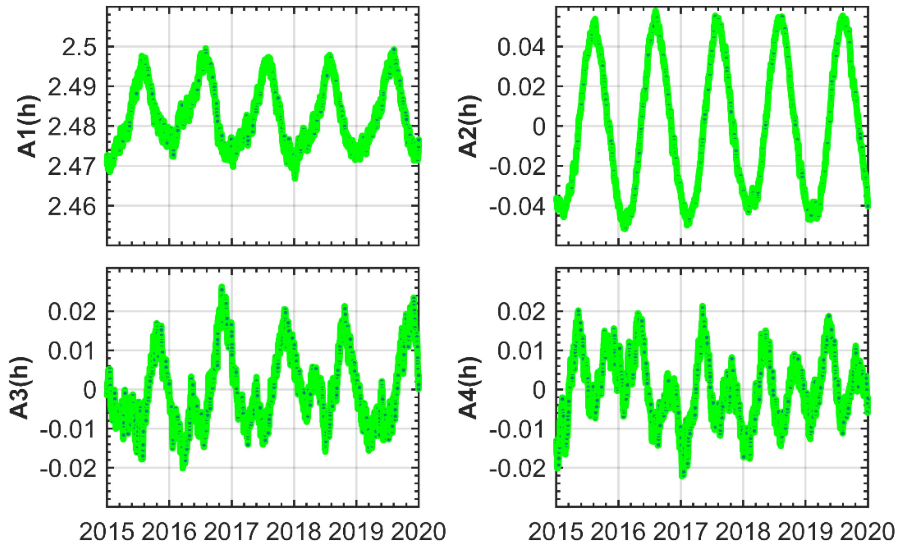
Figure 1 shows the time series of the first four orders coefficient Ai(h). As such, coefficient Ai(h) reflects the average variation in the tropospheric SH coefficients. The chart shows that coefficient Ai(h) exhibits obvious annual and semiannual cycles, and coefficients A3(h) and A4(h) also exhibit obvious quarterly variations. Through high-precision modeling of coefficient Ai(h), the SH coefficient is accurately inverted, and the high-precision tropospheric delay can then be obtained quickly and efficiently.

Figure 1.
Time series of the first four orders correlation coefficient from 2015 to 2019. The resolution of the time series is 1-h, and the width of each gray grid is one year in the x-axis direction.
Cooley and Tukey [31] proposed fast Fourier transform (FFT), which is usually used to analyze linear systems and identify frequency components. To accurately detect the period of correlation coefficient Ai(h), we performed the FFT analysis of the first four orders coefficient Ai(h) from 2015 to 2019 and focused on certain positions to obtain more details, as shown in Figure 2. The chart reveals that Ai(h) is dominated by both annual, semiannual, diurnal, and semidiurnal variations. In addition, A1(h) exhibits certain 1/3-year variation, A2(h) experiences certain 1/4-year variation, and A3(h) and A4(h) reveal certain 1/3-year and1/4-year variations.
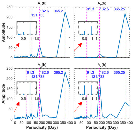
Figure 2.
Spectral analysis of the four orders correlation coefficients from 2015 to 2019. The block in the figure represents a short-time power spectrum. The blue font represents the period corresponding to the high-power spectrum.
3.2. EGtrop Model Construction
Based on the analysis in the previous section, Ai(h) exhibits obvious periodic characteristics, and the periods of the different parameters are distinct. Therefore, we use trigonometric functions with different periods to model EGtrop. The specific fitting equation is as follows:
where , , doy is the day of the year and Hod is the universal time (UT). Moreover, ai, bi, ci, di, ei and fi are all unknown parameters, which can be solved by the least-squares method. Please refer to Appendix A for the detailed establishment process.
The retrieve of Ai(h) can be achieved with a few coefficients, and then, the reconstruction of the SH coefficients also can be realized by using Equation (7). Only by giving doy and Hod, the user can obtain 256 tropospheric SH coefficients and the global tropospheric delay based on the mean sea level can be obtained by using the SH function. The global altitude correction coefficient is obtained by the same method. Finally, the ZTD at the specified position is obtained by Equation (5).
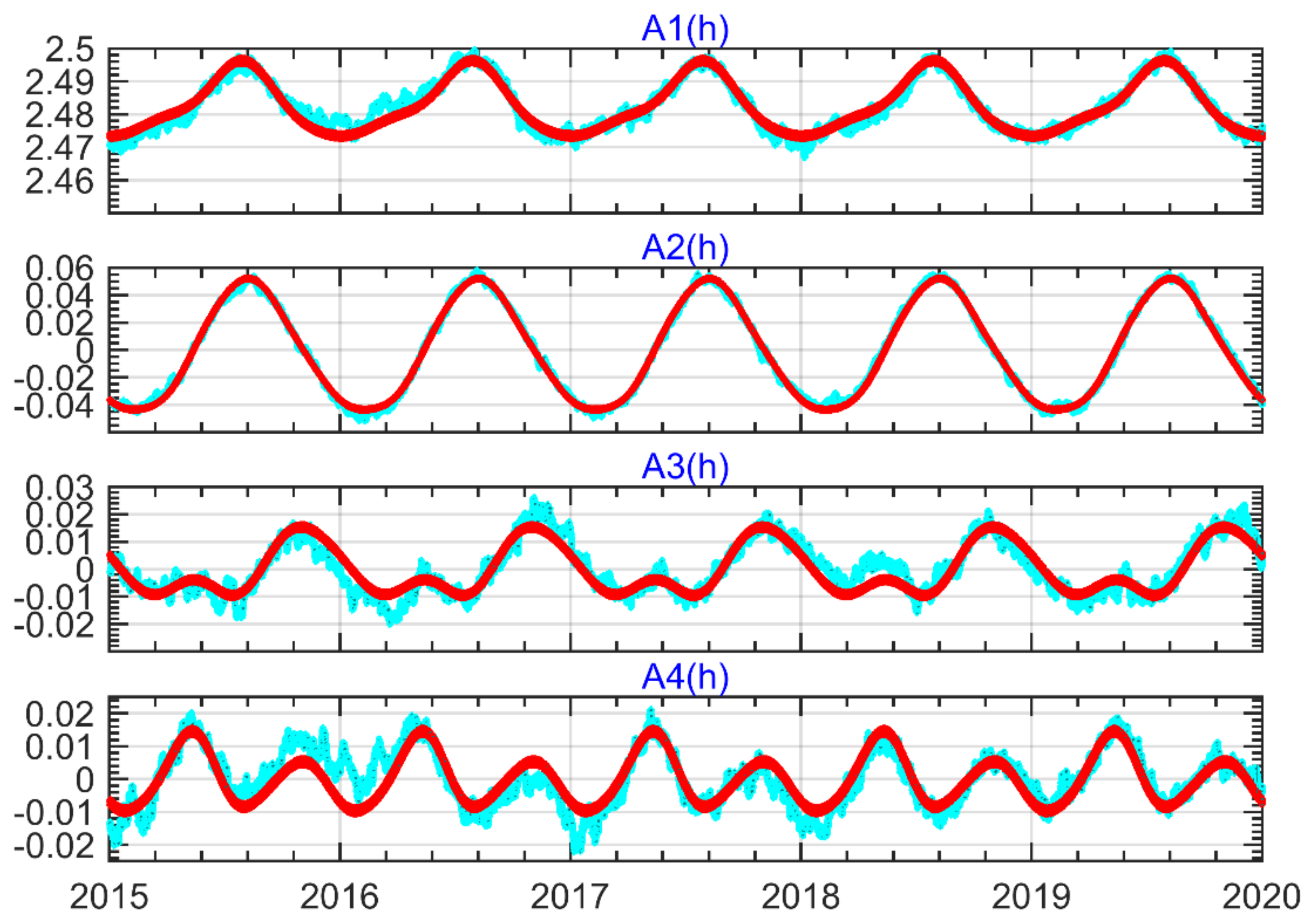
Figure 3 shows the time series diagram of the first four orders EOF parameters and fitting parameters. It can be seen from the figure that the trigonometric function achieves a better fitting effect on Ai(h).
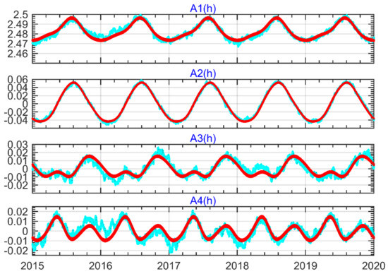
Figure 3.
Time series diagram of the first four orders EOF parameters and fitting parameters. Red dots indicate the fitting data, and cyan dots indicate the metadata.
4. Results
To assess the performance of the SH_set and EOF-based model EGtrop, we compared the set and model results with the ZTD derived from the IGS stations and radiosonde data. The mean Bias and root mean square error (RMSE) are adopted as accuracy indicators of the model or data quality. The calculation equation is as follows:
where ZTDmod and ZTDdat are the model value and the reference value, respectively. M is the number of observations.
4.1. Global Tropospheric Delay SH Coefficients Set Validation
In this contribution, the tropospheric delay calculated by the ERA-5 meteorological data from 2015 to 2019 and the tropospheric delay in 2018 of the IGS stations that did not participate in modeling are employed as reference data to verify the accuracy of the SH_set datasets.
Table 2 summarizes the statistical results of the Bias and RMSE of the SH_set datasets compared to ZTD derived from ERA-5. The table indicates that the average Bias in the SH_set dataset is very small and almost zero, the average RMSE is 1.97 cm, and the error remains almost the same in the different years, indicating that the SH_set dataset has a good fitting effect and can suitably describe the spatiotemporal characteristics of the global tropospheric delay.
Table 2.
Error statistics of the SH_set dataset compared to the ERA-5 ZTD.
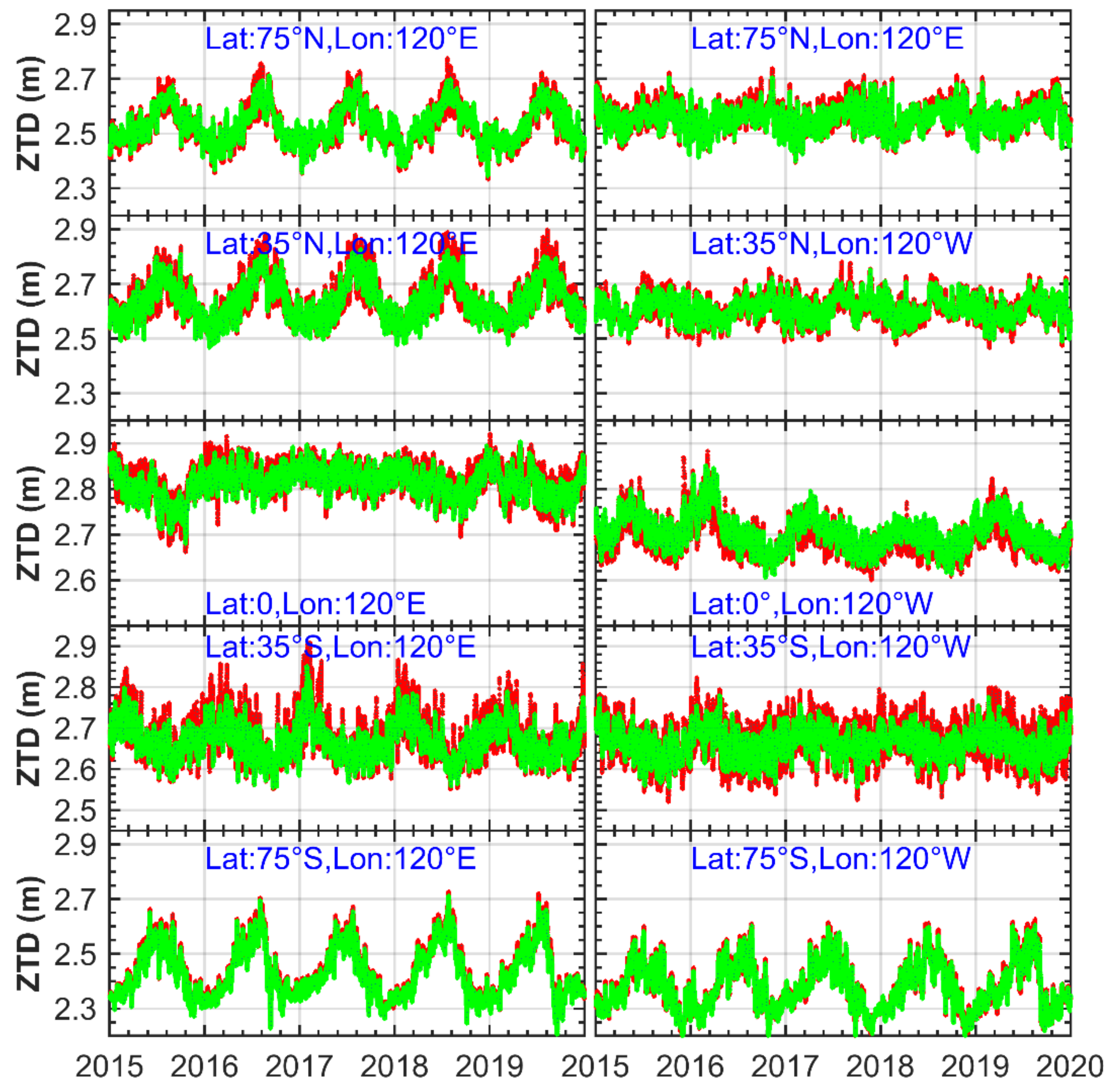
More detailed verification of the SH_set products is conducted from the perspective of time. Figure 4 shows the time series diagram of the ZTD at the different latitudes solved by ERA-5 and the SH_set. The chart shows that although there exist significant differences in the tropospheric delay between the different latitudes, the tropospheric delay values calculated by the SH_set reflect the periodic changes and are in good agreement with those of the ERA-5 ZTD, which further verifies that the spherical harmonic coefficient model achieves a good adaptability.

Figure 4.
Tropospheric delay sequence diagram solved by ERA-5 and SH_set. Red spots indicate the tropospheric delay of the ERA-5 solution, and green spots indicate the tropospheric delay of the SH_set solution.
High-precision IGS tropospheric delay products are reliable data to verify the accuracy of other tropospheric delay data or models. In this paper, IGS stations with an annual data volume of not fewer than 120 days are selected for comparison to the SH_set datasets, and the Bias and RMSE between these datasets are calculated.
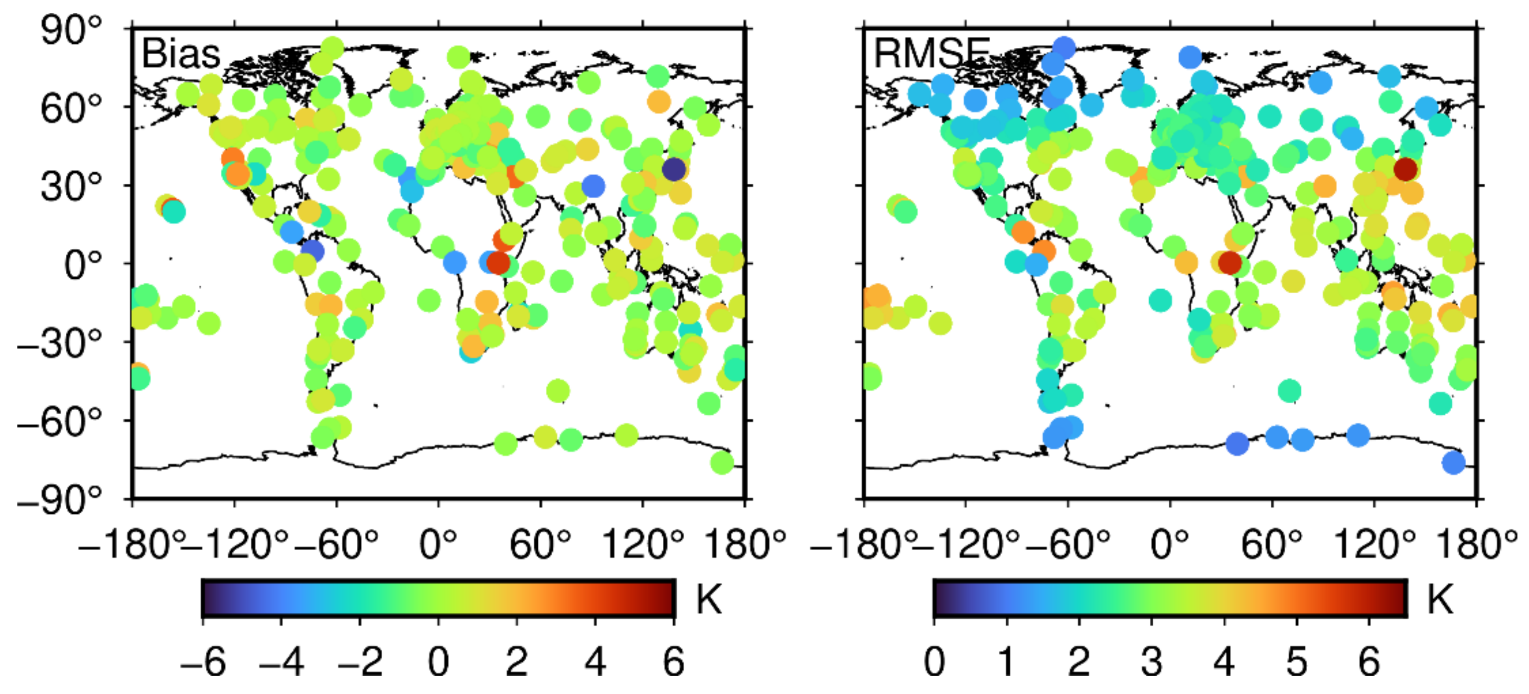
Figure 5 shows the error distribution of the SH_set data compared to the global IGS stations in 2018. The coincidence between the SH_set and IGS ZTD is high, the global distribution of the Bias is highly uniform, and the average Bias is 0.8 mm. The maximum and minimum values of the Bias are 4.4 cm and −4.6 cm, respectively, indicating that the tropospheric delay calculated by the SH_set yields good global applicability. The stations with large Bias are mainly concentrated in the low latitudes, especially those along the coast. In addition, the Bias values in the middle and high latitudes of the Northern and Southern Hemispheres are almost all positive, and the Bias in the area near the equator includes both positive and negative values.
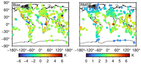
Figure 5.
Error distribution map of the SH_set data compared to the global IGS stations in 2018. The left side of the picture is the Bias distribution diagram, and the right side is the RMSE distribution diagram.
The RMSE ranges from 0.94 to 4.58 cm, with an average value of 2.61 cm, and the distribution is relatively uniform in the Northern and Southern Hemispheres. Several stations with RMSEs greater than 4 cm are mostly distributed near the equator, especially in the Atlantic Ocean. This is related to the different effects of the marine climate and geographical location on the ZTD on the east and west sides of the equator, while the SH_set, as an empirical dataset, is insensitive to this effect. Based on the verification of the IGS_ZTD data, the accuracy of the SH_set products (Bias: 0.8 mm; RMSE: 2.61 cm) is slightly lower than that of the Global Geodetic Observing System (GGOS) tropospheric delay products (Bias: −0.54 cm; RMSE: 1.31 cm) [32]. GGOS grid products spatial resolution is 2.5°(longitude) × 2° (latitude) and the temporal resolution is 6 h, i.e., 13,195 (145 × 91) ZTD data at a time. Compared to the GGOS products, the number of parameters of the SH_set products per day is reduced by approximately 94%, which is more convenient for users.
In summary, compared with the tropospheric delay calculated by ERA-5, SH data has a good performance in retrieving tropospheric delay, which further shows the feasibility of being a complement to the original data. Moreover, in comparison with IGS tropospheric delay products, it can be seen that the SH_set dataset attains a good global correction effect and can be used as a tropospheric delay product by users.
4.2. Verification of SH Coefficient for EGtrop Model
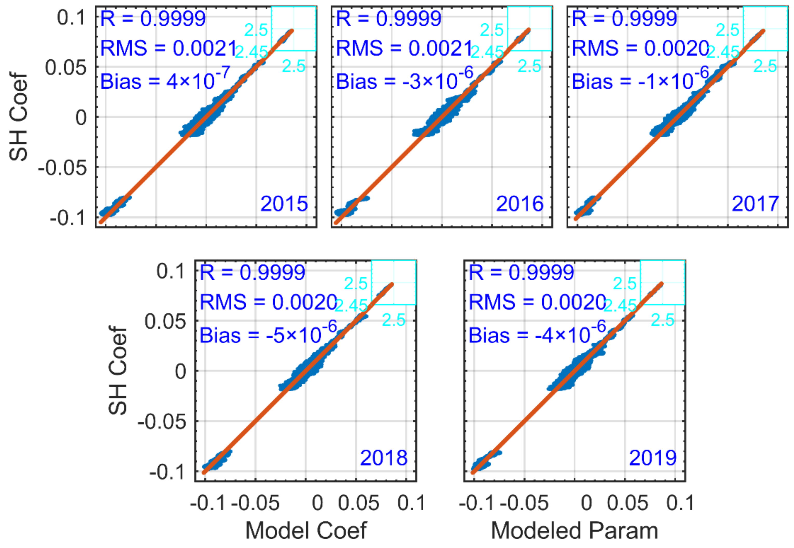
To test the stability and reliability of the EGtrop model, we use the SH coefficients provided by the SH_set to verify and analyze the EGtrop. Figure 6 displays scatter plots of SH provided by the SH_set and modeled values of SH from 2015 to 2019. In all years, the correlation coefficients R of the SH coefficients provided by the EGtrop and SH_set are all greater than 0.99, which means the model value has a strong correlation with the original value, indicating that the EGtrop model is appropriate for representing the majority of variations in the original data set. Bias and RMSE are very stable in all years. RMSE is basically 0.002 and the Bias is basically 0, indicating that the EGtrop has no systematic deviation, which further shows that the EGtrop model has a good performance in retrieving spherical harmonic coefficients.
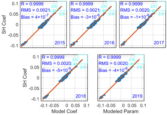
Figure 6.
Scatter plots of observational data versus modeled values of SH coefficients for the period 2015−2019. The blue-green box shows the first spherical harmonic coefficient. The correlation coefficient (R), RMSE (RMS) and Bias (Mean) are also shown in the panels.
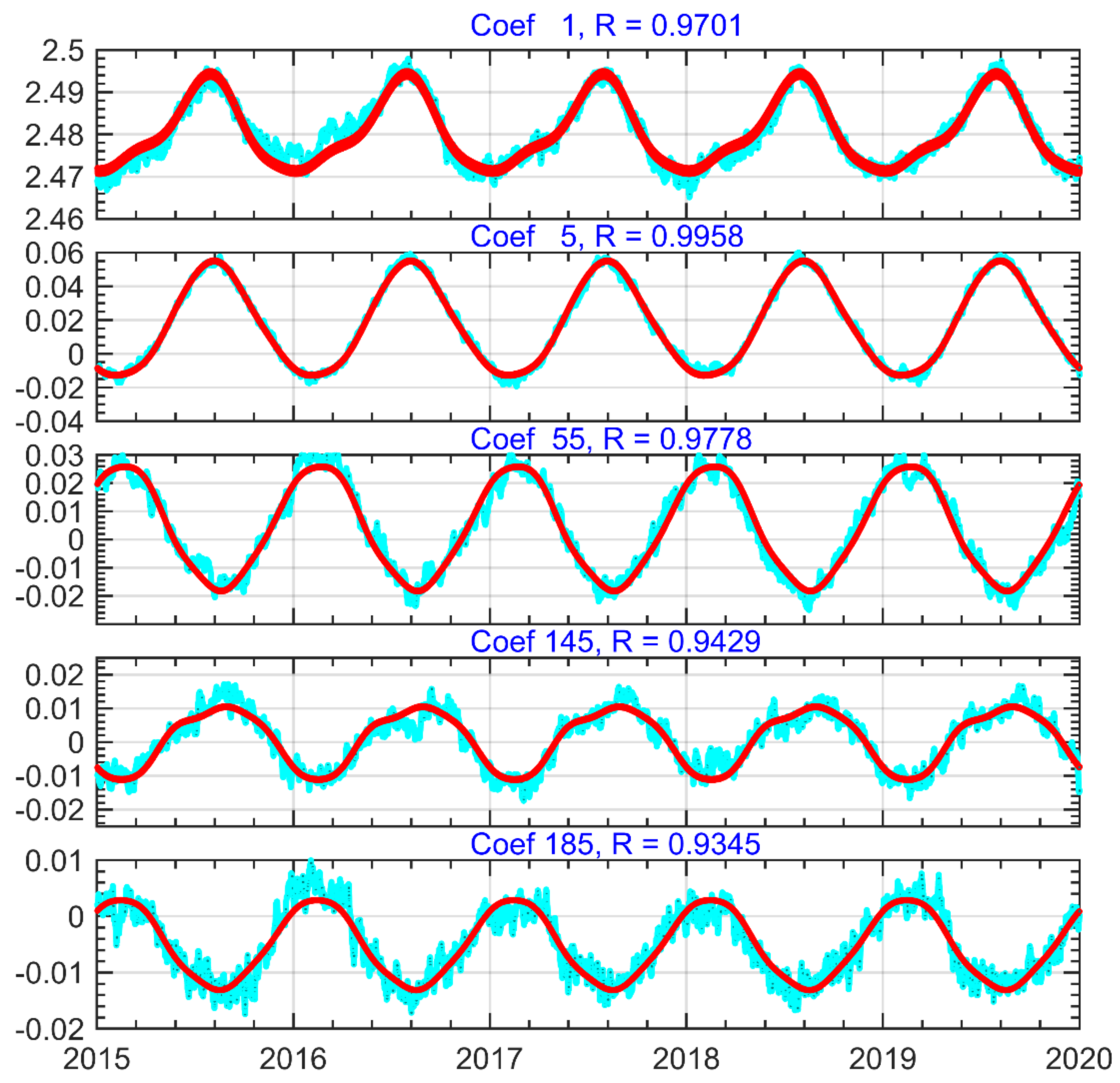
To further illustrate the reliability of the SH coefficients calculated by the EGtrop model, we randomly select five coefficients and display their time series, as shown in Figure 7. Figure 7 shows the first SH coefficient with larger values, and Figure 7 shows the SH coefficient with smaller values. It can be found from the figure that the EGtrop has a good performance in both large and small values of the SH coefficient. The correlation coefficient R of each SH coefficient is greater than 0.9, indicating that the SH coefficients calculated by the EGtrop are in good agreement with the original coefficient.

Figure 7.
Time series of SH coefficients between EGtrop and SH_set for the period 2015−2019. Cyan spots represent SH coefficients provide by SH_set, and red spots represent SH coefficients derived by EGtrop.
4.3. Verification of the Tropospheric Delay for EGtrop Model
In this study, the tropospheric delay calculated based on ERA-5 meteorological data and radiosonde data and IGS tropospheric delay products are considered to verify the EGtrop model. To objectively verify the validity of the EGtrop model, the UNB3m model and GPT2w (1° × 1°) model are introduced, and the accuracy is evaluated and analyzed under the same conditions.
Table 3 lists the statistical results of the Bias and RMSE of each model compared to those of the tropospheric delay calculated by the ERA-5 meteorological data in 2020. The table indicates that the accuracy of the EGtrop model is better than that of the GPT2w and UNB3m models, and the estimated tropospheric delay is the closest to that obtained with the ERA-5 ZTD. Compared to the other two models, the EGtrop model generates the smallest error fluctuation range, which indicates that the model achieves better stability.
Table 3.
Modeling errors of the different models validated against ERA-5 ZTD over 2020.
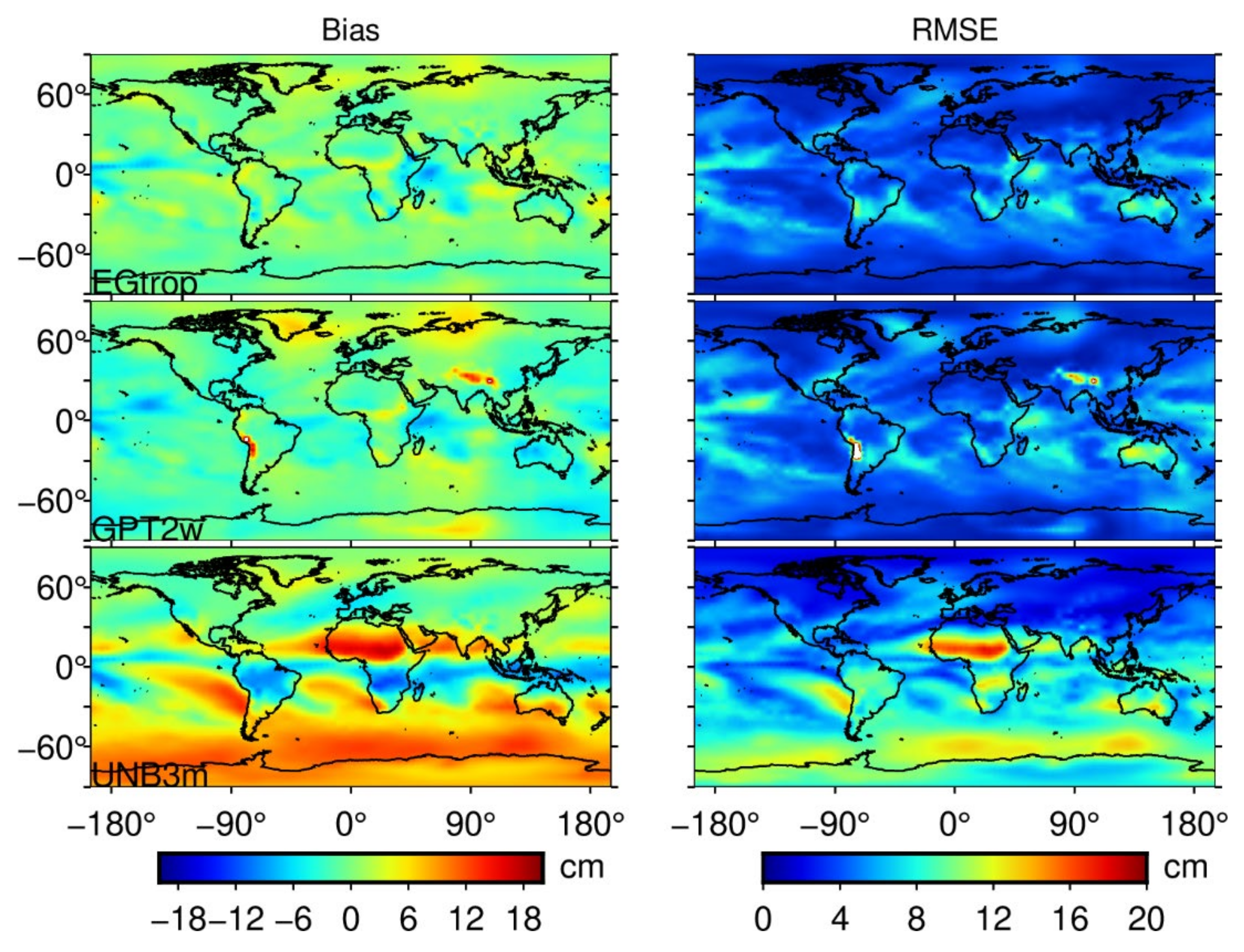
Figure 8 shows the global distribution of the annual average Bias and average RMSE of each model based on the global ERA-5 ZTD in 2020. As shown, the overall Bias of the EGtrop model is small, and the Bias value in most areas is 2 cm, which is closer to the reference value than are the GPT2w and UNB3m models.
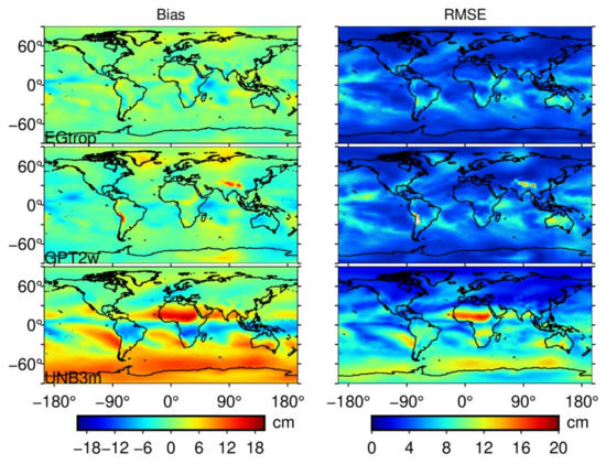
Figure 8.
Error distribution map of each model compared to the global ERA-5 ZTD product over 2020. The left side of the picture is the Bias distribution diagram, and the right side is the RMSE distribution diagram. From top to bottom are the error distributions of the EGtrop, GPT2w and UNB3m.
By comparing the Bias distribution of each model, it is revealed that the average Bias of the EGtrop and GPT2w models experiences no obvious change with the longitude and latitude, and the accuracy of the UNB3m model in the Northern Hemisphere is higher than that in the Southern Hemisphere, which is related to the fact that the global tropospheric delay of the UNB model is symmetrical in the north and south by default, and only the Northern Hemisphere data are used for the model. A larger Bias of the EGtrop model occurs in Antarctica and near the equator, especially in the Central Pacific and eastern Africa, and the value is negative. The Bias distribution of the EGtrop model is very uniform, and the overall Bias is smaller than that of the GPT2w model. Compared to the GPT2w model, the EGtrop model is much better in areas near the equator, especially in the Central Pacific region, the east and west sides of Africa, and the northern region of Australia.
By comparing the RMSE distribution of each model, it is found that the overall correction effect of the EGtrop model is better than that of the GPT2w and UNB3m models. By assessing Figure 8, it is found that the effect of the EGtrop model is better than that of the GPT2w model in the Southern Hemisphere, especially in the Antarctic and Australian regions. Larger RMSEs of the EGtrop and GPT2w models occur in the middle and low latitudes, and the maximum RMSE values are mainly distributed in the Central Pacific Ocean, western South America, and the Australian continent. This may be caused by two factors: on one hand, due to the severe variation in the tropospheric delay in the middle and low latitudes, the fitting effect is poor; on another, the tropospheric delay is affected by the land and sea distributions and topography. Among the three models, the RMSE of the UNB3m model with the lowest accuracy in the Northern Hemisphere is notably smaller than that in the Southern Hemisphere. It should be noted that the accuracy of the UNB3m model is similar to that of the GPT2w model in the high latitudes of the Northern Hemisphere.
In this study, the ZTD calculated by radiosonde stations and IGS, respectively, which does not participate in modeling in 2020, are used as reference data to verify the above model, and statistical analysis is carried out by the region. Table 4 lists the accuracy results of each model in each continental region compared to radiosonde and IGS. The table indicates that the accuracy of the model based on the different data sources varies, and the accuracy of the model verified against radiosonde data is relatively higher, which is related to the use of meteorological data for modeling. Among these models, the overall accuracy of the EGtrop model (Bias: 0.42 cm; RMSE: 3.65 cm) is equivalent to that of the GPT2w model (Bias: 0.04 cm; RMSE: 3.75 cm) model, which is better than that of the UNB3m model. The accuracy of the GPT2w model on all continents is slightly higher than that of the EGtrop model. The region with the largest RMSE difference between the two models is Oceania, with a difference of 6.9 mm. This is attributed to the low spatial resolution of the data source established by the EGtrop model (2° × 2°). The resulting inversion accuracy of the regional tropospheric delay is not as good as that of the high-resolution GPT2w model (1° × 1°). There are two main reasons for the poor accuracy of the models verified against the IGS ZTD data. On the one hand, this is caused by the systematic deviation between the different data sources. On the other hand, this is affected by the station location and data resolution, where the temporal resolution of the radiosonde is 12-h, and the temporal resolution of the IGS_ZTD is 1-h.
Table 4.
Error statistics of the tropospheric delay models compared to the ZTD derived from IGS and Radiosonde.
By comparing the accuracy between the different regions, it is found that the accuracy of the EGtrop model is higher than that of the GPT2w model in Europe and North America, while the accuracy in the other regions is the same. Through the above analysis, it is further demonstrated that the EGtrop model achieves good regional applicability. In addition, although the overall accuracy of the UNB3m model is not high, the accuracy of the model in Asia and Europe is similar to that of the other two models, which is related to the UNB3m modeling data and consistent with the experimental results of the previous section.
To validate the performance of the above models in different seasons, we statistically analyzed the monthly average results of the three models at global radiosonde stations. Figure 9 shows the monthly average Bias and RMSE of ZTD estimates between the models and radiosonde. As shown in the figure, EGtrop performs best with smaller absolute deviation and RMSE in different months when compared with other models. In terms of Bias for all months, the absolute average Bias of the three models in all months is within 1 cm, and the stability of the EGtrop model is better. The deviation of the EGtrop model in all months is positive, and the deviation of UNB3m is negative. In terms of RMSE for all seasons, the EGtrop model shows 0.16–2.5 cm and 6.52–13.84 cm improvements over the GPT2w and UNB3m models, respectively. Therefore, the performance of the EGtrop model is better than that of other models in different seasons. In addition, the RMSE of EGtrop, GPT2w, and UNB3m has obvious seasonal variations, and the accuracy in summer is usually lower than that in other seasons. This is because the water vapor content over the station changes sharply in summer, which leads to poor estimation results from the empirical model.
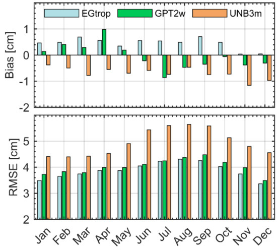
Figure 9.
Monthly Bias and RMSE for different models tested by radiosonde in 2020. Grey cyan, green and orange represents EGtrop, GPT2w and UNB3m, respectively. At the top of the figure is the distribution of the monthly average Bias of different models. The lower part of the figure shows the distribution of the monthly average RMSE of different models.
5. Conclusions
This study proposes a global tropospheric SH coefficient set (SH_set) and establishes a global SH coefficients empirical model, namely EGtrop based on EOF methods and periodic functions. The preliminary research results and conclusions are as follows:
- 1.
- This study adopts a spherical harmonic function to fit the tropospheric delay calculated with global ERA-5 meteorological data at each time, and an SH coefficients dataset is obtained in the calculation, which is convenient for EOF decomposition and formula fitting. It is verified that the SH_set yield a good accuracy (ERA-5 ZTD, Bias: −1.0 × 10⁻⁴ cm; RMSE: 1.97 cm; IGS ZTD, Bias: 0.08 cm; RMSE: 2.6 cm), indicating the feasibility and reliability of this strategy, which provides a reference for near-real-time model products.
- 2.
- Based on the analysis of the SH_set data from 2015 to 2019, it is found that the spherical harmonic coefficients exhibit a certain periodic variation. Based on this phenomenon, this study implements the EOF method and trigonometric functions to establish an SH coefficients model for the SH_set data called EGtrop and combines it with the spherical harmonic function to complete the establishment of the global tropospheric delay model. The results indicate that the accuracy of the new model is higher than that of GPT2w and UNB3m on the different reference data. In addition, through verification of the model accuracy, it is found that the EGtrop model is applicable not only at the global scale but also at the regional scale, and this model yields the advantage of local enhancement.
- 3.
- Compared to GGOS tropospheric delay grid data, the SH_set proposed in this study experiences a slight loss of accuracy, but it greatly reduces the number of parameters and is more convenient for users.
When the EOF and trigonometric functions are used to fit the spherical harmonic coefficients in this study, it is found that the fitting effect produces a large deviation in certain years. The improvement of the fitting effect of the spherical harmonic coefficients needs further study. In addition, the severe tropospheric delay in the middle and low latitudes, especially in the low latitudes of the Southern Hemisphere, greatly affects the accuracy of the model. The execution of high-precision tropospheric delay modeling in the middle and low latitudes should be further investigated.
Author Contributions
Data curation, H.L.; formal analysis, Y.M.; investigation, G.X.; methodology, Y.M.; software, Z.L.; validation, H.L.; writing—original draft, Y.M.; writing—review and editing, Z.L. All authors have read and agreed to the published version of the manuscript.
Funding
The project was financially supported by the Guangdong Basic and Applied Basic Research Foundation (Nos. 2021A1515012600) and the Shenzhen Science and Technology Program (Nos. KQTD20180410161218820).
Data Availability Statement
ECMWF reanalysis data can be obtained from the following website: https://apps.ecmwf.int/datasets/ (accessed on 29 April 2021). The meteorological data of sounding stations can be downloaded from the following link: ftp://ftp.ncdc.noaa.gov/pub/data/igra/ (accessed on 29 April 2021). The IGS product data files can be downloaded from the following website: ftp://geodesy.noaa.gov/ (accessed on 29 April 2021).
Acknowledgments
The authors would like to thank the ECMWF and Integrated Global Radiosonde Archive (IGRA) for providing the meteorological data and the IGS for providing the tropospheric delay products of IGS stations.
Conflicts of Interest
The authors declare no conflict of interest.
Appendix A
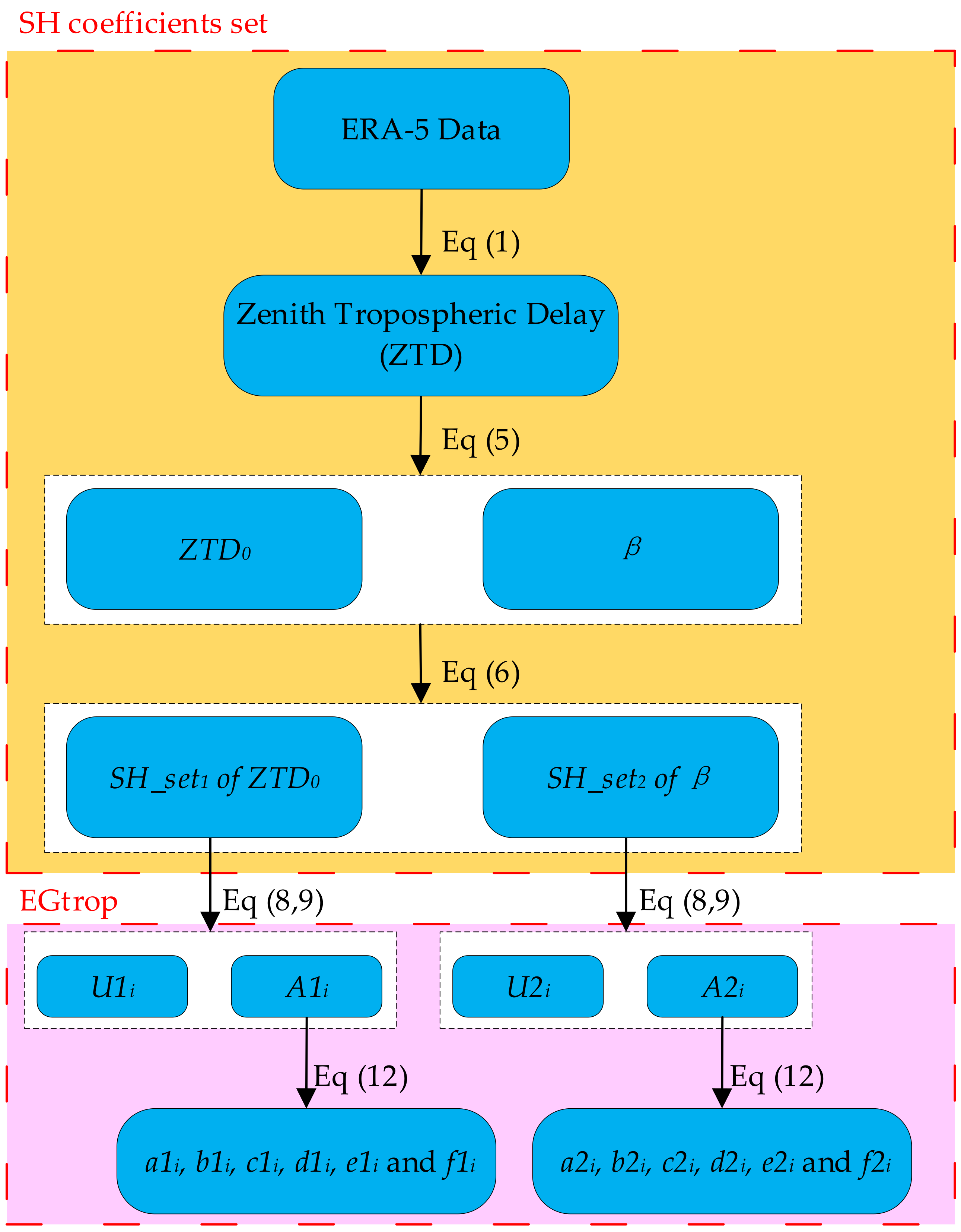
For the reader to be able to replicate the models are described, the data used in each stage and the process of building the model are further described, as shown in Figure A1. The modeling process in detail is as follows:
First, based on ERA-5 data from 2015 to 2019, the ZTD value is solved by Equation (1). Considering the influence of altitude on tropospheric delay, the tropospheric delay grid data is uniformly corrected to the grid data based on mean sea level by Equation (5), including ZTD0 and the corresponding altitude correction coefficient β.
Then, based on the global grid data (ZTD0 and β), the global tropospheric spherical harmonic coefficient set (SH_set) is established through the spherical harmonic function (Equation (6)).
Last, we decompose the SH_set by the EOF method (Equations (8) and (9)) to obtain the basis vectors (U) and corresponding coefficients (Ai(h)). The EGtrop model is established by time fitting (Equation (12)) the EOF coefficients (Ai(h)).
The reconstruction of the SH coefficients can be realized by using Equation (7). Only by giving doy and Hod, the user can get tropospheric SH coefficients. Then, the global tropospheric delay based on the mean sea level can be obtained by using the SH function and coefficients. The global altitude correction coefficient is obtained by the same method. Finally, the ZTD at the specified position is obtained by Equation (5).
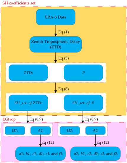
Figure A1.
Flowchart of EGtrop model construction.
Figure A1.
Flowchart of EGtrop model construction.
References
- Davis, J.L.; Herring, T.A.; Shapiro, I.I.; Rogers, A.E.E.; Elgered, G. Geodesy by radio interferometry: Effects of atmospheric modeling errors on estimates of baseline length. Radio Sci. 1985, 20, 1593–1607. [Google Scholar] [CrossRef]
- Askne, J.; Nordius, H. Estimation of tropospheric delay for microwaves from surface weather data. Radio Sci. 1987, 22, 379–386. [Google Scholar] [CrossRef]
- Ifadis, I.M. Space to earth techniques: Some considerations on the zenith wet path delay parameters. Survey Rev. 1993, 32, 130–144. [Google Scholar] [CrossRef]
- Tregoning, P.; Herring, T.A. Impact of a priori zenith hydrostatic delay errors on GPS estimates of station heights and zenith total delays. Geophys. Res. Lett. 2006, 33, 160–176. [Google Scholar] [CrossRef] [Green Version]
- Hopfield, H.S. Tropospheric Effect on Electromagnetically Measured Range: Prediction from Surface Weather Data. Radio Sci. 1971, 6, 357–367. [Google Scholar] [CrossRef]
- Saastamoinen, J. Atmospheric Correction for the Troposphere and Stratosphere in Radio Ranging Satellites. Use Artif. Satell. Geod. 1972, 15, 247–251. [Google Scholar] [CrossRef]
- Li, W.; Yuan, Y.; Ou, J.; Li, H.; Li, Z. A new global zenith tropospheric delay model IGGtrop for GNSS applications. Chin. Sci. Bull. 2012, 57, 2132–2139. [Google Scholar] [CrossRef] [Green Version]
- Böhm, J.; Möller, G.; Schindelegger, M.; Pain, G.; Weber, R. Development of an improved empirical model for slant delays in the troposphere (GPT2w). GPS Solut. 2015, 19, 433–441. [Google Scholar] [CrossRef] [Green Version]
- Collins, J.P.; Langley, R.B. A Tropospheric Delay Model for the User of the Wide Area Augmentation System; Contract report for Nav Canada by the Geodetic Research Laboratory, Department of Geodesy and Geomatics Engineering Technical Report No. 187; University of New Brunswick: Fredericton, NB, Canada, 1997. [Google Scholar]
- Collins, J.; Langley, R. The residual tropospheric propagation delay: How bad can it get? In Proceedings of the 11th International Technical Meeting of the Satellite Division of The Institute of Navigation (ION GPS 1998), Nashville, TN, USA, 15–18 September 1998; The Institute of Navigation: Washington, DC, USA, 1998; pp. 729–738. [Google Scholar]
- Li, W.; Yuan, Y.; Ou, J.; He, Y. IGGtrop_SH and IGGtrop_rH: Two Improved Empirical Tropospheric Delay Models Based on Vertical Reduction Functions. IEEE Trans. Geosci. Remote Sens. 2018, 56, 5276–5288. [Google Scholar] [CrossRef]
- Penna, N.; Dodson, A.; Chen, W. Assessment of EGNOS Tropospheric Correction Model. J. Navig. 2001, 54, 37–55. [Google Scholar] [CrossRef] [Green Version]
- Sun, Z.; Zhang, B.; Yao, Y. A Global Model for Estimating Tropospheric Delay and Weighted Mean Temperature Developed with Atmospheric Reanalysis Data from 1979 to 2017. Remote Sens. 2019, 11, 1893. [Google Scholar] [CrossRef] [Green Version]
- Xu, C.; Yao, Y.; Shi, J.; Zhang, Q.; Peng, W. Development of Global Tropospheric Empirical Correction Model with High Temporal Resolution. Remote Sens. 2020, 12, 721. [Google Scholar] [CrossRef] [Green Version]
- Sun, Z.; Zhang, B.; Yao, Y. An ERA5-Based Model for Estimating Tropospheric Delay and Weighted Mean Temperature Over China With Improved Spatiotemporal Resolutions. Earth Space Sci. 2019, 6, 1926–1941. [Google Scholar] [CrossRef]
- Zhang, S.; Wang, X.; Li, Z.; Qiu, C.; Zhang, J.; Li, H.; Li, L. A New Four-Layer Inverse Scale Height Grid Model of China for Zenith Tropospheric Delay Correction. IEEE Access 2020, 8, 210171–210182. [Google Scholar] [CrossRef]
- Pearson, K. LIII. On lines and planes of closest fit to systems of points in space. Lond. Edinb. Dublin Philos. Mag. J. Sci. 1901, 2, 559–572. [Google Scholar] [CrossRef] [Green Version]
- Dvinskikh, N.I. Expansion of ionospheric characteristics fields in empirical orthogonal functions. Adv. Space Res. 1988, 8, 179–187. [Google Scholar] [CrossRef]
- Mao, T.; Wan, W.; Yue, X.; Sun, L.; Zhao, B.; Guo, J. An empirical orthogonal function model of total electron content over China. Radio Sci. 2008, 43. [Google Scholar] [CrossRef]
- Zhang, M.L.; Liu, C.; Wan, W.; Liu, L.; Ning, B. A global model of the ionospheric F2 peak height based on EOF analysis. Ann. Geophys. 2009, 27, 3203–3212. [Google Scholar] [CrossRef] [Green Version]
- Ercha, A.; Zhang, D.H.; Xiao, Z.; Hao, Y.Q.; Ridley, A.J.; Moldwin, M. Modeling ionospheric foF2 by using empirical orthogonal function analysis. Ann. Geophys. 2011, 29, 1501–1515. [Google Scholar] [CrossRef] [Green Version]
- Ercha, A.; Zhang, D.; Ridley, A.J.; Xiao, Z.; Hao, Y. A global model: Empirical orthogonal function analysis of total electron content 1999–2009 data. J. Geophys. Res. Space Phys. 2012, 117, A03328. [Google Scholar] [CrossRef] [Green Version]
- Chen, Z.; Zhang, S.-R.; Coster, A.J.; Fang, G. EOF analysis and modeling of GPS TEC climatology over North America. J. Geophys. Res. Space Phys. 2015, 120, 3118–3129. [Google Scholar] [CrossRef]
- Le, H.; Yang, N.; Liu, L.; Chen, Y.; Zhang, H. The latitudinal structure of nighttime ionospheric TEC and its empirical orthogonal functions model over North American sector. J. Geophys. Res. Space Phys. 2017, 122, 963–977. [Google Scholar] [CrossRef]
- Andima, G.; Amabayo, E.B.; Jurua, E.; Cilliers, P.J. Modeling of GPS total electron content over the African low-latitude region using empirical orthogonal functions. Ann. Geophys. 2019, 37, 65–76. [Google Scholar] [CrossRef] [Green Version]
- Hersbach, H.; Dee, D. ERA5 reanalysis is in production. ECMWF Newslett 2016, 147, 5–6. [Google Scholar]
- Thayer, G.D. An improved equation for the radio refractive index of air. Radio Sci. 1974, 9, 803–807. [Google Scholar] [CrossRef]
- Li, S.; Xu, T.; Jiang, N.; Yang, H.; Wang, S.; Zhang, Z. Regional Zenith Tropospheric Delay Modeling Based on Least Squares Support Vector Machine Using GNSS and ERA5 Data. Remote Sens. 2021, 13, 1004. [Google Scholar] [CrossRef]
- Pavlis, N.K.; Holmes, S.A.; Kenyon, S.C.; Factor, J.K. The development and evaluation of the Earth Gravitational Model 2008 (EGM2008). J. Geophys. Res. Solid Earth 2012, 117. [Google Scholar] [CrossRef] [Green Version]
- Uwamahoro, J.C.; Habarulema, J.B. Modelling total electron content during geomagnetic storm conditions using empirical orthogonal functions and neural networks. J. Geophys. Res. Space Phys. 2015, 120, 11000–11012. [Google Scholar] [CrossRef]
- Cooley, J.W.; Tukey, J.W. An Algorithm for the Machine Calculation of Complex Fourier Series. Math. Comput. 1965, 19, 297–301. [Google Scholar] [CrossRef]
- Yao, Y.; Xu, X.; Hu, Y. Precision Analysis of GGOS Tropospheric Delay Product and Its Application in PPP. Acta Geod. Cartogr. Sin. 2017, 46, 278–287. [Google Scholar] [CrossRef]


Publisher’s Note: MDPI stays neutral with regard to jurisdictional claims in published maps and institutional affiliations. |
© 2021 by the authors. Licensee MDPI, Basel, Switzerland. This article is an open access article distributed under the terms and conditions of the Creative Commons Attribution (CC BY) license (https://creativecommons.org/licenses/by/4.0/).