Abstract
Satellite quantitative precipitation estimation (QPE) can make up for the insufficiency of ground observations for monitoring precipitation. Using an Advanced Geosynchronous Radiation Imager (AGRI) on the FengYun-4A (FY-4A) satellite and rain gauges (RGs) for observations in the summer of 2020. The existing QPE of the FY-4A was evaluated and found to present poor accuracy over the complex topography of Western China. Therefore, to improve the existing QPE, first, cloud classification thresholds for the FY-4A were established with the dynamic clustering method to identify convective clouds. These thresholds consist of the brightness temperatures (TBs) of FY-4A water vapor and infrared channels, and their TB difference. Then, quantitative cloud growth rate correction factors were introduced to improve the QPE of the convective-stratiform technique. This was achieved using TB hourly variation rates of long-wave infrared channel 12, which is able to characterize the evolution of clouds. Finally, the dynamic time integration method was designed to solve the inconsistent time matching between the FY-4A and RGs. Consequently, the QPE accuracy of the FY-4A was improved. Compared with the existing QPE of the FY-4A, the correlation coefficient between the improved QPE of the FY-4A and the RG hourly precipitation increased from 0.208 to 0.492, with the mean relative error and root mean squared error decreasing from −47.4% and 13.78 mm to 8.3% and 10.04 mm, respectively. However, the correlation coefficient is not sufficiently high; thus, the algorithm needs to be further studied and improved.
1. Introduction
Precipitation plays an important role in the interaction of the hydrosphere, atmosphere and biosphere [1,2,3,4]; its uneven spatial and temporal distribution often lead to extreme weather events such as rainstorms and drought, which have a serious impact on human activities [5,6,7]. Therefore, it is vital to obtain accurate and timely spatial-temporal information of precipitation for meteorological study, flash flood monitoring, water resource management, climatological modeling and assessing groundwater storage [8,9,10]. In addition, the accurate acquisition of precipitation intensity and accumulated precipitation is conducive to understanding the global water cycle and the energy balance of the Earth system [11].
Rain gauges (RGs) are the most direct and common precipitation detection equipment, which have a high accuracy at specific locations [12,13]. However, due to the limited regional representativeness of single station observation, when the distribution of RGs is sparse, there is insufficiency in estimating the spatial distribution of precipitation by RGs only [14]. By comparison with radar observation, Smith et al. [15,16] indicated that it is difficult to depict the intensity and spatial extent of heavy precipitation, even if the RG observation network is relatively dense. Furthermore, in the process of heavy precipitation, due to the influence of wind and the mechanical limitations of the bucket RGs, it is easy to obtain inaccurate catches [17,18]. To a certain extent, a weather radar solves the above problems and provides a continuous precipitation observation with a high spatial-temporal resolution, which plays an important role in the study of local precipitation spatial-temporal distributions. Nevertheless, ground-based weather radars are not the preference for large-scale precipitation observations because of the limitations of the observation range and the significant costs associated with equipment purchase and maintenance [19]. Ground-based weather radars often encounter beam blocking caused by terrain (particularly over complex topography such as hills and mountains), which brings uncertainty to radar quantitative precipitation estimation (QPE) [20,21,22].
Satellites can cover a wide range of observation, and their precipitation products provide an opportunity for QPE in areas with few RGs, which can not only describe the spatial-temporal changes of precipitation in these areas, but also have considerable accuracy [23,24]. Since the 1990s, the development of meteorological satellite detection technology has made up for the lack of spatial distribution of RGs and radar detection, and this makes it possible to establish reliable and cost-effective precipitation datasets [7,25,26]. Satellite-derived precipitation products also play a significant role in the monitoring and analysis of the rainstorm process [27].
Currently, satellite-derived precipitation products are mainly based on geostationary (GEO) satellites, low earth orbiting (LEO) satellites and the combination of multi-satellite observations. Although the microwave scanning radiometer carried by LEO satellites has a strong penetrability in the cloud and rain atmosphere and can directly obtain precipitation structure information, it is usually confined to precipitation retrievals over the ocean. The strong low-frequency upwelling radiation on land surfaces can submerge the low-frequency radiation emitted by precipitation particles; therefore, the low-frequency microwave channel is difficult to use for land surface precipitation retrieval [27]. Concurrently, due to the low temporal resolution, the low-frequency microwave channel has no advantage in the continuous observation of precipitation. Similarly, the rain radar carried by LEO satellites has the same limitation. Nevertheless, the application of near-real-time satellite QPE is expected for disaster preparedness and mitigation on both a regional and global scale [28]. Therefore, in view of the shortage of RGs, limited radar coverage due to terrain impact and low temporal resolution of LEO satellites, it is crucial to carry out QPE based on GEO satellites for monitoring and early warning of short-term heavy precipitation.
The precipitation retrieval of GEO satellites is mainly based on visible (VIS) and infrared (IR) channels. Barrett [29] carried out early precipitation estimation by using daily IR and VIS band cloud image data. Although the spatial resolution of VIS images is the highest, it is only limited to daytime. Therefore, the precipitation retrieval of GEO satellites is mainly based on IR images. The reason why IR cloud images can be used for remote sensing of rainstorm cloud is that when the brightness temperature (TB) of cloud-top IR radiation is lower, the higher the cloud top’s height, the thicker the cloud body, and the thickness of the cloud body is positively correlated with the probability of precipitation [30]. Wang et al. [31] and Zhuge et al. [32] constructed a generic matrix of two-dimensional precipitation probability and precipitation intensity based on the MTSAT and FengYun-2C (FY-2C) satellites, respectively, to realize the precipitation retrieval for different levels of rainfall. Moreover, many studies have shown that there is a good relationship between satellite IR TB and surface rainfall rates, especially for convective clouds, and the methods of QPE by satellite IR brightness temperatures (TBs) have been developed [33,34,35]. A benchmark technique is the GOES Precipitation Index (GPI), which simply allocates a rainfall rate of 3 mm/h to clouds with a cloud-top temperature lower than 235 K [36]. Based on the principle of the GPI algorithm, Ba and Gruber [37] proposed another automatic algorithm for GOES, the GOES multispectral rainfall algorithm (GMSRA), which adds a VIS light albedo threshold to identify precipitation clouds, and improves the recognition rate of warm cloud precipitation in the daytime. After the rainfall rate is retrieved by the IR secondary fitting method, the humidity factor is introduced for adjustment. Although such methods are subject to uncertainty due to the indirect relationship between the cloud-top temperature to surface precipitation, it has proved useful for operational use in the United States [38]. The National Environmental Satellite Data and Information Service (NESDIS) of the National Oceanic and Atmospheric Administration (NOAA) began carrying out QPE by satellite data in the 1970s, mainly with the manual Interactive Flash Flood Analyzer [39], which was automated into an auto-estimator (AE) after 10 years of operation [35,40] and then improved by a hydro-estimator (HE) [41]. Finally, the advantages of a microwave-estimated rainfall rate were combined with GOES data with high spatial and temporal resolution, and a self-calibrating multivariate precipitation retrieval (SCaMPR) algorithm was developed for the Geostationary Operational Environmental Satellite R series (GOES-R) [42]. Because different types of precipitation clouds produce different rainfall rates, Adler and Negri [34] proposed a convective-stratiform technique (CST) for QPE based on a one-dimensional cloud model, which can both estimate convective cloud precipitation and stratiform cloud precipitation. Subsequently, this algorithm is widely adopted for QPE and the estimation is in good agreement with ground observation [43,44,45,46,47]. In addition, artificial intelligence is also used in satellite QPE [48,49,50,51]. However, the effect of artificial intelligence is highly dependent on the overall quality of the training samples and data used, particularly as the model needs to be trained or tagged, and the training of high-resolution satellite images requires substantial computing resources [52]; therefore, artificial intelligence is currently not the optimal choice for satellite QPE.
The FengYun-4A (FY-4A) satellite, the first satellite of the FengYun-4 (FY-4) series of China’s second-generation GEO meteorological satellites, was launched on 11 December 2016, with a central longitude of 104.7°E [53]. Compared with the existing FengYun-2 (FY-2) satellite, the imaging observation channels of the advanced geosynchronous radiation imager (AGRI) carried on the FY-4A are expanded from 5 to 14, and more information about precipitation clouds can be obtained, which is conducive to the monitoring of short-term heavy precipitation. As Feng Yun satellites are the major operational meteorological satellites of China, the application of its QPE product becomes more necessary. It remains a challenge to use the FY-4A AGRI data for QPE. Compared with the FY-2 and GMS-5, the number of observation channels of the FY-4 has increased significantly, and the temporal resolution is higher; however, there are few studies of QPE based on FY-4 observations, and it is important to evaluate the existing QPE of the FY-4A and improve its accuracy, especially over complex topography. This paper introduces an application method of FY-4A AGRI multi-channel spectral data in QPE and evaluates its effect with complex topography in Western China. Section 2 introduces the dataset and methods used for QPE validation, while Section 3 describes the validation of the existing QPE of the FY-4A and the improvement of the QPE algorithm based on the FY-4A AGRI, as well as the accuracy of the improved QPE, and the discussion of the results is presented in Section 4. Conclusions are drawn in Section 5.
2. Materials and Methods
China’s topography is high in the west and low in the east, roughly in three-step terrains. The first-step terrain: the Qinghai-Tibet Plateau located in southwest China, with an average altitude of more than 4000 m. The second-step terrain: to the north and east of the outer edge of the Qinghai-Tibet Plateau; it is mainly composed of broad plateaus and basins, and there are also a series of high mountains, most of which are at an average altitude of 1000–2000 m. The third-step terrain: from the second step to the east to the seashore; it is mainly composed of hills, low mountains and plains, and the altitude is mostly below 500–1000 m. The three-step terrains form a variety of topographic features, including mountains (such as Tibetan Plateau), hills, plains and basins [19]. This study focuses on the region of 24° to 34°E and 100° to 112°N in Western China. As shown in Figure 1, this region has a complex topography covering the above three-step terrains. Due to the complex topography, rainstorm events occur frequently in this area, often leading to natural disasters such as floods, debris flow and landslides [54,55,56].
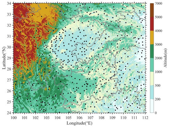
Figure 1.
The topography and distribution of RGs (black dots) in the study region.
From June to August 2020, the precipitation in the study region, and its downstream, were more than that in the same period from previous years, and most rainstorms were related to the Southwest Vortex, which also originated in this region [57,58,59]. Therefore, we selected data from June to August 2020 for this study. As mentioned above, the shortage of the RGs and limited radar coverage due to the terrain impact can easily arise in Western China with its complex topography; therefore, it is important to carry out QPE by GEO satellite observations for monitoring and early warning of short-term heavy precipitation in this region. This study only focused on summer precipitation, and we were only looking at the relationship between temperature and precipitation for convective clouds. It should be noted that the area is only covered by 508 national RGs.
The hourly precipitation of the 508 national RGs used in this study was obtained from the China Integrated Meteorological Information Sharing Service platform (CIMISS). As shown in Figure 1, the average station spacing is about 50 km. This dataset has been subject to quality control, and the actual rate is more than 99.9%, while the data accuracy is close to 100% [60]. The real-time QPE of the FY-4A AGRI from the National Satellite Meteorological Center (NSMC) used in this study was issued by the fourth edition of the Meteorological Information Comprehensive Analysis and Processing System (MICAPS 4.0), with a spatial resolution of 0.04° × 0.04°and temporal resolution of 15 min.
Compared with the FY-2, the imaging channels of the FY-4A AGRI are expanded from 5 to 14, and the observation time is encrypted from 30 min to 15 min while the spatial resolution is improved from 1.25 km to 500 m. In particular, the FY-4A AGRI has two water vapor (WV) channels and four longwave infrared (LWIR) bands (as shown in Table 1), which can obtain more information on precipitation clouds. With the advantages of high spatial-temporal resolution, and more information on precipitation clouds, the FY-4A AGRI is conducive to the monitoring of short-term heavy precipitation. As heavy precipitation in Western China mostly occurs in the summer, the above data from June to August of 2020 were used in this study.

Table 1.
The two WV (water vapor) and four LWIR (long-wave infrared) channel settings of the FY-4A AGRI.
To match the RG hourly precipitation and QPE of the FY-4A AGRI, the principle of proximity and the method of taking the mean value were adopted as follows: first, to avoid the uncertainty of weak precipitation, only an RG hourly precipitation greater than 5 mm was used in this study (The CST algorithm gives stratiform cloud precipitation a fixed rainfall intensity, generally 2 or 2.5 mm/h). Because our research object was heavy precipitation, this threshold of 5 mm/h was to reduce the impact of weak precipitation); second, at a fixed RG station, all effective QPE data within one hour and 20 km away from the station were matched, but only the QPE with the closest value to the RG hourly precipitation was selected. Finally, there were 2790 matched couples selected from June to August of 2020.
As the most commonly used statistical data in satellite estimation verification, continuous verification statistics are often used to measure the accuracy of precipitation [61]. Six popular diagnostic statistics (Table 2) were used to evaluate the agreement between the RGs and QPE of the FY-4A [19,61,62,63,64,65,66]. The degree of agreement is represented by the correlation coefficient (CC), which is independent of absolute or conditional bias, and represents the degree of linear correlation between QPE and RGs, whose optimal value is 1. As for error and bias, five different validation statistical indices were considered. The mean error (ME) reflects the average difference between QPE and RGs, while the mean absolute error (MAE) represents the average magnitude of the error, and their optimal values are 0. The root mean square error (RMSE) suggests the degree of dispersion between QPE and RGs but the larger errors contribute more than the MAE, and the optimal value is also 0. The percentage deviations of QPE from RGs are indicated by the mean relative error (MRE) and mean absolute relative error (MARE), which are scale-independent, are useful for comparing different datasets, and their optimal values are 0. For convenience, the acronyms used in this study are listed in Table A1 in the Appendix A .
Table 2.
List of the validation statistical indices used to compare the QPE of the FY-4A AGRI and the GRs.
3. Results
3.1. Validation of NSMC QPE
To validate the real-time QPE of the FY-4A AGRI provided by NSMC, Figure 2 presents the comparison between RG hourly precipitation and NSMC QPE of the FY-4A AGRI from June to August of 2020 in Western China. As shown in Figure 2a, all hourly QPEs are less than 30 mm, the ME is a negative value of −8.48 mm, and the scatter clustering trend of data is lower than the diagonal of 1:1 and far away, indicating that the NSMC QPE is obviously underestimated relative to the RG hourly precipitation. The CC between RGs and QPE is only 0.208, with values of 13.78 mm, 9.13 mm, −47.4%, and 56.9% for RMSE, MAE, MRE and MARE, respectively, indicating poor agreement and a large discrepancy between RGs and QPE. Although the ME has an average value of −8.48 mm, about 30% of the ME values are less than −10 mm (Figure 2b). The MRE ranges from −100% to 100% with an average value of −47.4%, and more than 65% of the MRE values are less than −50%. Apparently, the existing QPE of the FY-4A AGRI is underestimated and presents poor agreement with RG hourly precipitation greater than 5 mm over the complex topography of Western China; therefore, it is necessary to study the improvement of the QPE algorithm for the FY-4A AGRI.
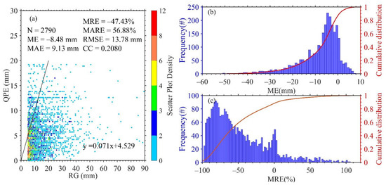
Figure 2.
Comparison between RG hourly precipitation and NSMC QPE of the FY-4A AGRI from June to August of 2020 in Western China: (a) scatter density plot, (b) PDF and CDF of ME and (c) PDF and CDF of MRE.
3.2. Improvement of QPE Algorithm Based on the FY-4A AGRI
3.2.1. Cloud Classification
Since there are differences in the precipitation mechanism of different precipitation clouds, it is necessary to identify and classify clouds effectively for improving the satellite QPE algorithm.
Presently, there are three main methods for cloud classification based on GEO satellite data. One is the cloud classification method of the American GOES-R satellite [67], which classifies the cloud phase state by combining the TB of LWIR channel 12 (10.8 μm) and the TB difference between the WV channel 10 (7.1 μm) and LWIR channel 11 (7.1 μm), as well as the TB difference between WV channel 10 and LWIR channel 12 (hereinafter referred to as Method 1). The second is the single channel multi-threshold method [68]. This method uses the TB of LWIR channel 12 to classify cloud types (hereinafter referred to as Method 2). The third is the dynamic clustering method [69], which composes the cloud cluster center to classify the cloud types by combining the TB values of WV channel 9 (6.25 μm), LWIR channel 12 and LWIR channel 13 (12 μm), as well as the TB difference between WV channel 9 and LWIR channel 12 (hereinafter referred to as Method 3).
Figure 3 shows the cloud classification of the above three methods and the hourly precipitation at 08:00 LST on 1 July 2020 in Western China. In general, the ground heavy precipitation center is consistent with the convective cloud positions and deep convective clouds in the three cloud classification methods, and the shape of the rain belt is also consistent, indicating that the identification results for convective clouds and deep convective clouds in Methods 1–3 are basically consistent. However, the identification result of Method 3 is relatively more accurate than the other two methods; thus, Method 3 was adopted in this study to classify clouds. Moreover, to take advantage of the large number of channels of the FY-4A AGRI, this study increased the number of channels in Method 3, and the used channel TBs and the TB difference thresholds for cloud classification based on the FY-4A AGRI are shown in Table 3.
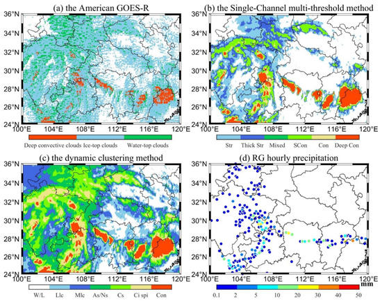
Figure 3.
Cloud classification of (a) Method 1, (b) Method 2, and (c) Method 3 and (d) the hourly precipitation at 08:00 LST on July 1, 2020, in Western China. (Str: Stratiform clouds, Thick Str: Thick stratiform clouds, Mixed: Mixed clouds, SCon: Shallow convective clouds, Con: Convective clouds, Deep Con: Deep convective clouds, W/L: Water/Land surface, Llc: Low level clouds, Mlc: Middle level clouds, As/Ns: Altostratus/Nimbostratus clouds, Cs: Cirrostratus clouds, Ci spi: Cirrus spissatus clouds).
Table 3.
The used channel TB and TB difference thresholds for cloud classification based on the FY-4A AGRI.
3.2.2. Improvements of QPE Algorithm
Based on the cloud classification of the FY-4A AGRI, the CST algorithm of Adler and Negri [34] is used to perform the QPE of the FY-4A AGRI. According to the exponential relationship between convective cloud-top temperature and rainfall rate [43,44,45,46,47], the RG hourly precipitation data from June to August in 2020 is fitted with the corresponding TB data of the FY-4A AGRI 12 channel to obtain the localized relationship for calculating the primary FY-4A QPE product. Figure 4 presents the plots of the RG hourly precipitation with the cloud-top temperature of LWIR channel 12 and the primary FY-4A QPE from June to August of 2020. As shown in Figure 4a, the cloud-top temperature presents a decreasing trend with the increasing ground hourly precipitation, and this supports the basis for satellite QPE. As the ground hourly precipitation increases, the cloud-top temperature decreases gradually, especially below 30mm. The difference of cloud-top temperature in precipitation above 30 mm is small, and this is the reason why it is difficult to better identify heavy precipitation with the GEO satellite QPE. Comparing the existing NSMC QPE of the FY-4A (Figure 2a), Figure 4b shows that the CC between the primary FY-4A QPE and the RG hourly precipitation increases slightly to 0.232, and the ME between them is reduced to 2.59 mm. However, the MRE between the primary FY-4A QPE and the RG hourly precipitation is 86.2%, greater than that of the NSMC QPE of the FY-4A. It can be seen that the primary FY-4A QPE is still not satisfied and needs further improvement.
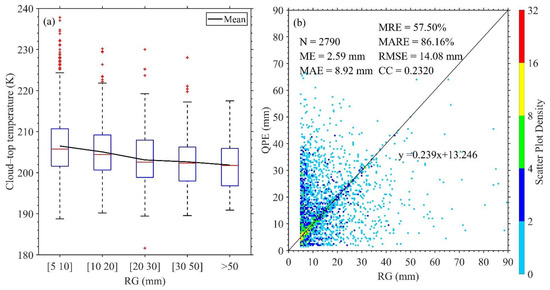
Figure 4.
The plots of the RG hourly precipitation vs (a) the cloud-top temperature of LWIR channel 12 and (b) the primary FY-4A QPE from June to August of 2020 (In Figure 4a, bottom and top of boxes denote the 25th and 75th percentiles, with the horizontal lines inside the box being the median value; the dotted lines represent the range of the adjacent value, which is the most extreme value that is not an outlier; the outliers are marked by crosses).
As the CST algorithm only considers the TB spatial gradient of a cloud cluster for the selection of a convective cloud core and uses the instantaneous cloud-top TB for precipitation retrieval. The temporal variation of cloud-top TB is not considered in this algorithm, which can accurately reflect the evolution of clouds. Some studies have shown that the cloud growth rate (i.e., the change of cloud-top TB in two continuous infrared images) and spatial gradient are useful for locating the core of heavy precipitation [35]. Compared with the FY-2, the temporal resolution of the FY-4A is greatly improved, which supports an opportunity to apply the temporal variation of TB in satellite QPE.
Considering the special scanning mode of the FY-4A, and the time matching with hourly precipitation, the hourly variation rate of TB, i.e., the TB difference between the current time and one hour before, is used to investigate the relationship between TB variability and hourly precipitation. In order to eliminate the influence of water or land surface and low level clouds, the TB of IR channel 12 of less than 270 K was used as the cloud criterion in this study (referring to this criterion, only 4 of the 364,477 ground surface temperature samples were lower than 270 K and might be misidentified as cloud), and the TB of the RG station is represented by the average of the TBs within 20 km around in one hour. Figure 5 presents the relationship between the hourly precipitation and the hourly variation rate of TB for WV channel 9 and LWIR channel 12; with the increase in hourly precipitation, the hourly variation rate of TB for WV channel 9 is negative and its magnitude increases, that is, the TB at the cloud top decreases with time and decreases faster with the increasing hourly precipitation. Similarly, this is the same situation—and the effect is more significant—for the hourly variation rate of TB for LWIR channel 12. However, the relationships of the hourly precipitation with the TBs of the other channels are not significant (figures not shown). Thus, the TBs of LWIR channel 12 were used to improve the CST algorithm for calculating the secondary QPE.
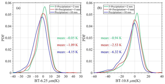
Figure 5.
The relationship between the hourly precipitation and the hourly variation rate of TB for (a) WV channel 9 and (b) LWIR channel 12 from June to August of 2020.
According to the method of the AE [35], the cloud growth rate correction factor is quantified by linearly fitting the positive and negative rainfall rate variability with the TB variability of LWIR channel 12 in one hour, respectively. Thus, based on the primary FY-4A QPE (QPEP), the secondary FY-4A QPE (QPES) was calculated by adding TB temporal variation according to the following formula:
where Ti,j is the TB of LWIR channel 12 at the location of (i, j), and ΔTi,j, min(Ti,j) and max(Ti,j) are the average variability of Ti,j, the minimum Ti,j and the maximum Ti,j within one hour at this location, respectively. In the processing of the correction, if QPES has a value above 0.5 mm, then QPEP is replaced by QPES; otherwise, QPEP remains unchanged.
Note that the research on satellite precipitation retrieval is mostly based on the precipitation in one hour or even longer, but the satellite observation is instantaneous, so the inconsistency of observation methods in time matching can bring errors to satellite precipitation retrieval. In order to solve this problem, the dynamic time integration method was adopted in this study; that is, according to the comparison between the QPE at the current time and the QPE at the previous or subsequent time, the time integration weight X is determined as the following formula:
where QPE0 is the instantaneous QPE at the current time (T0) obtained from the CST algorithm, and QPE−1 and QPE1 are the instantaneous QPE at the previous (T−1) and subsequent (T1) times, respectively. The dynamic time integration method is shown in Figure 6—the number of bars represents QPE; the blue and green bar represents QPE−1 and QPE1, respectively, assuming that the five grey bars represent QPE0 and remain constant. The ideal state is that the three QPEs are equal and, in this case, no processing is required. In addition to the ideal state, the processing methods of the other four cases are as follows: (1) when QPE0 is greater than QPE−1 and QPE1, the time integration weights for the previous and subsequent times increase; (2) when QPE0 is smaller than QPE−1 and QPE1, the time integration weight for the previous and subsequent times decrease; (3) when QPE0 is greater than QPE−1 but smaller than QPE1, the time integration weight decreases at the previous time yet increases at the subsequent time; (4) when QPE0 is smaller than QPE−1 but greater than QPE1, the time integration weight increases at the previous time yet decreases at the subsequent time.
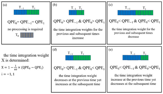
Figure 6.
Dynamic time integration method (a) the ideal state, (b) both smaller than, (c) both greater than (d) front smaller than rear greater than, and (e) front greater than rear smaller than and dynamic time integration coefficient (the number of bars represents QPE, blue and green bars represent QPE-1 and QPE1, respectively, assuming that the five grey bars represent QPE0 and remain constant).
After the time integration weight X is calculated, the hourly QPE is obtained by combining X with the instantaneous QPE and accumulating it within one hour, and then the TB hourly variation rate of LWIR channel 12 is used to correct the hourly QPE. Thus, the improved QPE (QPEI) is calculated according to the following formula:
where Δ Time is the time interval of two consecutive IR images, and the other variables are the same as in Equations (1) and (2).
Therefore, the whole QPE-improved algorithm flow is as follows: first, the optimized multi-channel and channel difference thresholds are used to identify convective clouds, and the primary QPE is calculated by the CST algorithm; second, the TB temporal variation of LWIR channel 12 is used to improve the CST algorithm, and the secondary QPE is calculated; finally, the dynamic time integration method is adopted to solve the inconsistency of time matching, and the secondary QPE at the current time, as well as those at the previous and subsequent times, are used to calculate the improved QPE with time integration weight.
3.3. Validations of Improved QPE Algorithm Based on the FY-4A AGRI
Figure 7 presents the scatter density plots of the RG hourly precipitation with the secondary QPE and the improved QPE from June to August of 2020. It can be seen that the CC between RGs and the primary FY-4A QPE is only 0.232, and the MRE and RMSE are 57.5% and 14.08 mm, respectively (Figure 4b). After adding the TB temporal variation of LWIR channel 12, the CC increases to 0.476 for the secondary QPE, with MRE and RMSE decreasing to 23.8% and 10.51 mm, respectively. The CC between the RGs and improved QPE further increases to 0.492, and the MRE and RMSE further decrease to 8.3% and 10.04 mm, respectively, when the dynamic time integration method is used. Moreover, compared with the primary QPE, both the overestimation for hourly precipitation less than 10 mm and the underestimation for hourly precipitation within 20–30 mm are improved to some extent in the improved QPE. This is mainly because the temporal variation of TB can provide a more accurate quantitative description of the development trend of clouds, which can effectively avoid the overestimation of QPE caused by some low TB clouds with a short life history, so as to improve the estimation accuracy of QPE. As pointed out by Vicente et al. [35], not considering the evolution of the cloud system can result in an excessive area of precipitation by using the IR cloud-top temperature alone for QPE. Furthermore, the introduction of TB temporal variation can do well for improving the accuracy of QPE, while the dynamic time integration method is also useful for reducing the uncertainty of QPE caused by the temporal inconsistency of the data.
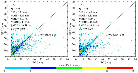
Figure 7.
The scatter density plots of the RG hourly precipitation vs (a) the secondary FY-4A QPE and (b) the improved FY-4A QPE from June to August of 2020 in Western China.
4. Discussion
The NSMC QPE of the FY-4A is not satisfactory for summer precipitation over the complex topography of Western China. This may be related to the fact that the NSMC QPE of the FY-4A is a national product that focuses on the whole national region and lacks specific validation over complex topography. Moreover, the precipitation mechanisms of various rain types are different, and the inconsistent time matching of data also brings uncertainty in satellite QPE. Therefore, to improve the QPE accuracy of the FY-4A, in this study the dynamic clustering method was used to perform cloud classification, and the TB spatio-temporal variation was adopted to represent the evolution of precipitation clouds. Moreover, the dynamic time integration method was used to reduce the uncertainty of time mismatching for data coupling. Next, the QPE of the FY-4A was improved and showed good agreement with the surface RG hourly precipitation. Compared with the NSMC QPE of the FY-4A, the CC between the RG hourly precipitation and the improved QPE increased from 0.208 to 0.492, and the MRE and RMSE decreased from −47.4% and 13.78 mm to 8.3% and 10.04 mm respectively. It was also found that the two WV channels of the FY-4A and their channel difference could well give the evolution characteristics of water vapor in the middle and upper atmosphere, which may be a good indicator of precipitation, especially heavy precipitation. These results show that the high temporal resolution of the FY-4 is useful for improving satellite QPE accuracy.
It should be noted that there is no clear standard for the test of cloud classification. This study only makes a simple qualitative verification of precipitation clouds based on the hourly precipitation of RGs, and there may be confusion between cirrus and convective clouds. Additionally, the improved QPE algorithm is mainly based on cloud-top temperature for precipitation retrieval, which is not suitable for warm cloud precipitation. After adopting the improved algorithm, the correlation coefficient has been improved, as well as the accuracy. However, the correlation coefficient is not sufficiently high, which indicates that the satellite QPE still has uncertainty; thus, the algorithm needs to be further studied and improved.
Ba and Gruber [37] indicated that the precipitation process in warm clouds is sensitive to the microphysical structure at the top, and the occurrence and development of precipitation are affected by cloud droplet size and cloud thickness. The microphysical process of the cloud top can be obtained from the near-infrared part of the solar spectrum [70], and the 3.75 μm channel of the Advanced Very High Resolution Radiometer (AVHRR) has been proven to be suitable for the study of warm cloud precipitation [71,72]. Moreover, the multi-channel TB differences (such as T3.9-T10.8, T3.9-T7.3, T8.7-T10.8, and T10.8-T12.1) have been found to contain the information of cloud liquid water path [73]. Thus, in future work, the 3.72 μm medium-wave IR (MWIR) channel can be used to improve the QPE algorithm of FY-4 series satellites.
5. Conclusions
Using the hourly precipitation of 508 national RG stations from June to August in 2020, the NSMC QPE products of the FY-4A over the complex topography of Western China were evaluated, and an improved QPE algorithm was derived by using the multi-channel spectral data of the FY-4A AGRI with a high spatial and temporal resolution. The main conclusions are as follows.
The NSMC QPE of the FY-4A is underestimated and presents poor accuracy for an hourly precipitation greater than 5 mm over Western China. It has a CC of only 0.208 with RG hourly precipitation, and the MRE and RMSE between them are −47.4% and 13.78 mm, respectively. All the NSMC QPE are less than 30 mm and obviously underestimated for heavy precipitation. The poor accuracy of NSMC QPE may be related to the fact that the NSMC QPE of the FY-4A is a national product that focuses on the whole national region and lacks specific investigation over complex topography.
To improve the QPE of the FY-4A, the dynamic clustering method was adopted to establish the cloud classification thresholds with WV channel TB and IR channel TB of the FY-4A AGRI and their TB difference for identifying convective clouds. Moreover, to take advantage of the high temporal resolution of the FY-4A, the hourly variation rates of TB of LWIR channel 12 were introduced to the CST algorithm for characterizing cloud evolution. Furthermore, a dynamic time integration method was designed to solve the inconsistency of time matching between the FY-4A and RGs. The QPE accuracy of the FY-4A was then significantly improved. Compared with the NSMC QPE of the FY-4A, the CC between the improved QPE of the FY-4A and the RG hourly precipitation increased to 0.492, and decreased to 8.3% and 10.04 mm with MRE and RMSE, respectively. However, the correlation coefficient was not sufficiently high, thus the algorithm needs to be further studied and improved.
These results indicate that the high temporal resolution and multi channels of the FY-4A are useful for improving satellite QPE. However, this study only makes simple qualitative verification of precipitation clouds, and there may be confusion between cirrus and convective clouds, which may bring uncertainty to satellite QPE. In addition, the improved QPE algorithm in this study is mainly based on cloud-top temperature and not suitable for warm cloud precipitation. Therefore, different QPE improvement schemes may be required for different terrains and different precipitation types.
Author Contributions
Conceptualization, Y.X., G.X. and R.W.; methodology, J.R. and W.Z.; software, L.L. and Y.X.; validation, J.R. and W.Z.; formal analysis, J.R. and W.Z.; investigation, J.R.; resources, J.R.; data curation, J.R., W.Z. and J.W.; writing—original draft preparation, J.R.; writing—review and editing, J.R., W.Z. and G.X.; visualization, J.R. and W.Z.; supervision, G.X., Y.X. and R.W.; project administration, R.W. and Y.X.; funding acquisition, R.W. All authors have read and agreed to the published version of the manuscript.
Funding
This research was funded by the National Key Research and Development Program of China (2018YFC1507201), the National Natural Science Foundation of China (41620104009) and the Science and Technology Foundation of Hubei Meteorological Bureau (2021Q03).
Data Availability Statement
Not applicable.
Acknowledgments
The authors’ great gratitude is extended to the NSMC for providing the FY-4A data and its product data used in this study. We would like to thank the China Meteorological Administration (CMA) for providing the RG data. We also appreciate the NOAA / National Geophysical Data Center (NGDC) for providing the Etopo1 terrain data.
Conflicts of Interest
The authors declare no conflict of interest.
Appendix A
Table A1.
Acronym list for the acronyms used in this study (arrange in alphabetical order).
Table A1.
Acronym list for the acronyms used in this study (arrange in alphabetical order).
| Abbreviate | Full Name |
|---|---|
| AE | auto-estimator |
| AGRI | Advanced Geosynchronous Radiation Imager |
| AVHRR | Advanced Very High Resolution Radiometer |
| CC | correlation coefficient |
| CDF | cumulative distribution function |
| CIMISS | China Integrated Meteorological Information Sharing Service platform |
| CST | convective-stratiform technique |
| FY-2 | Fenyun-2 |
| FY-4A | Fengyun-4A |
| GEO | geostationary |
| GMSRA | GOES multispectral rainfall algorithm |
| GOES-R | Geostationary Operational Environmental Satellite R series |
| GPI | GOES precipitation index |
| HE | hydro-estimator |
| IR | infrared |
| LEO | low earth orbiting |
| LWIR | long-wave infrared |
| LST | local standard time |
| MAE | mean absolute error |
| MARE | mean absolute relative error |
| ME | mean error |
| MICAPS | Meteorological Information Comprehensive Analysis and Processing System |
| MRE | mean relative error |
| MWIR | medium-wave infrared |
| NESDIS | National Environmental Satellite Data and Information Service |
| NOAA | National Oceanic and Atmospheric Administration |
| NSMC | National Satellite Meteorological Center |
| probability density function | |
| QPE | quantitative precipitation estimation |
| RG | rain gauge |
| RMSE | root mean squared error |
| SCaMPR | self-calibrating multivariate precipitation retrieval |
| TB | brightness temperature |
| WV | water vapor |
| VIS | visible |
References
- Kidd, C.; Huffman, G. Global precipitation measurement. Meteorol. Appl. 2011, 18, 334–353. [Google Scholar] [CrossRef]
- Allen, M.R.; Ingram, W.J. Constraints on future changes in climate and the hydrologic cycle. Nature 2002, 419, 228–232. [Google Scholar] [CrossRef]
- Yong, B.; Liu, D.; Gourley, J.J.; Tian, Y.; Huffman, G.J.; Ren, L.; Hong, Y. Global View Of Real-Time Trmm Multisatellite Precipitation Analysis: Implications For Its Successor Global Precipitation Measurement Mission. Bull. Am. Meteorol. Soc. 2015, 96, 283–296. [Google Scholar] [CrossRef]
- Tang, G.; Ma, Y.; Long, D.; Zhong, L.; Hong, Y. Evaluation of GPM Day-1 IMERG and TMPA Version-7 legacy products over Mainland China at multiple spatiotemporal scales. J. Hydrol. 2016, 533, 152–167. [Google Scholar] [CrossRef]
- Futrell, J.; Gephart, R.; Kabat-Lensch, E.; McKnight, D.; Pyrtle, A.; Schimel, J.; Smyth, R.; Skole, D.; Wilson, D.; Gephart, J. Water: Challenges at the Intersection of Human and Natural Systems; 2005. Available online: https://www.osti.gov/biblio/1046481 (accessed on 29 October 2021). [CrossRef]
- Council, N.R. When Weather Matters: Science and Services to Meet Critical Societal Needs; National Academies Press: Washington, DC, USA, 2010; pp. 60–70. ISBN 13 978-0-309-15249-5. [Google Scholar]
- Kucera, P.A.; Ebert, E.E.; Turk, F.J.; Levizzani, V.; Kirschbaum, D.; Tapiador, F.J.; Loew, A.; Borsche, M. Precipitation from Space: Advancing Earth System Science. Bull. Am. Meteorol. Soc. 2013, 94, 365–375. [Google Scholar] [CrossRef]
- Trenberth, K.E.; Smith, L.; Qian, T.; Dai, A.; Fasullo, J. Estimates of the Global Water Budget and Its Annual Cycle Using Observational and Model Data. J. Hydrometeorol. 2007, 8, 758–769. [Google Scholar] [CrossRef]
- Hegerl, G.C.; Black, E.; Allan, R.P.; Ingram, W.J.; Polson, D.; Trenberth, K.E.; Chadwick, R.S.; Arkin, P.A.; Sarojini, B.B.; Becker, A.; et al. Challenges in Quantifying Changes in the Global Water Cycle. Bull. Am. Meteorol. Soc. 2015, 96, 1097–1115. [Google Scholar] [CrossRef]
- Ruhi, A.; Messager, M.L.; Olden, J.D. Tracking the pulse of the Earth’s fresh waters. Nat. Sustain. 2018, 1, 198–203. [Google Scholar] [CrossRef]
- Hou, A.Y.; Kakar, R.K.; Neeck, S.; Azarbarzin, A.A.; Kummerow, C.D.; Kojima, M.; Oki, R.; Nakamura, K.; Iguchi, T. The Global Precipitation Measurement Mission. Bull. Am. Meteorol. Soc. 2014, 95, 701–722. [Google Scholar] [CrossRef]
- New, M.; Todd, M.; Hulme, M.; Jones, P. Precipitation measurements and trends in the twentieth century. Int. J. Climatol. 2001, 21, 1889–1922. [Google Scholar] [CrossRef]
- Villarini, G.; Mandapaka, P.V.; Krajewski, W.F.; Moore, R.J. Rainfall and sampling uncertainties: A rain gauge perspective. J. Geophys. Res. Atmos. 2008, 113, D11102. [Google Scholar] [CrossRef]
- Woldemeskel, F.M.; Sivakumar, B.; Sharma, A. Merging gauge and satellite rainfall with specification of associated uncertainty across Australia. J. Hydrol. 2013, 499, 167–176. [Google Scholar] [CrossRef]
- Smith, J.A.; Bradley, A.A.; Baeck, M.L. The Space-Time Structure of Extreme Storm Rainfall in the Southern Plains. J. Appl. Meteorol. Climatol. 1994, 33, 1402–1417. [Google Scholar] [CrossRef]
- Smith, J.A.; Seo, D.J.; Baeck, M.L.; Hudlow, M.D. An Intercomparison Study of NEXRAD Precipitation Estimates. Water Resour. Res. 1996, 32, 2035–2045. [Google Scholar] [CrossRef]
- Groisman, P.; Legates, D. The Accuracy of United States Precipitation Data. Bull. Am. Meteorol. Soc. 1994, 75, 215–227. [Google Scholar] [CrossRef]
- Peck, E.L. Quality of Hydrometeorological Data in Cold Regions. JAWRA J. Am. Water Resour. Assoc. 1997, 33, 125–134. [Google Scholar] [CrossRef]
- Xu, J.; Ma, Z.; Tang, G.; Ji, Q.; Min, X.; Wan, W.; Shi, Z. Quantitative evaluations and error source analysis of Fengyun-2-based and GPM-based precipitation products over mainland China in summer, 2018. Remote Sens. 2019, 11, 2992. [Google Scholar] [CrossRef]
- Kitchen, M.; Brown, R.; Davies, A.G. Real-time correction of weather radar data for the effects of bright band, range and orographic growth in widespread precipitation. Q. J. R. Meteorol. Soc. 1994, 120, 1231–1254. [Google Scholar] [CrossRef]
- Westrick, K.J.; Mass, C.F.; Colle, B.A. The Limitations of the WSR-88D Radar Network for Quantitative Precipitation Measurement over the Coastal Western United States. Bull. Am. Meteorol. Soc. 1999, 80, 2289–2298. [Google Scholar] [CrossRef]
- Pellarin, T.; Delrieu, G.; Saulnier, G.-M.; Andrieu, H.; Vignal, B.; Creutin, J.-D. Hydrologic Visibility of Weather Radar Systems Operating in Mountainous Regions: Case Study for the Ard?che Catchment (France). J. Hydrometeorol. 2002, 3, 539–555. [Google Scholar] [CrossRef]
- Li, X.; Zhang, Q.; Xu, C.-Y. Assessing the performance of satellite-based precipitation products and its dependence on topography over Poyang Lake basin. Theor. Appl. Climatol. 2014, 115, 713–729. [Google Scholar] [CrossRef]
- Jongjin, B.; Jongmin, P.; Dongryeol, R.; Minha, C. Geospatial blending to improve spatial mapping of precipitation with high spatial resolution by merging satellite-based and ground-based data. Hydrol. Process. 2016, 30, 2789–2803. [Google Scholar] [CrossRef]
- Levizzani, V.; Bauer, P.; Joseph Turk, F. Measuring Precipitation from Space: EURAINSAT and the Future; Springer: Dordrecht, The Netherlands, 2007; Volume 28, pp. 49–58. ISBN 13 978-1-4020-5835-6. [Google Scholar] [CrossRef]
- Shukla, S.; McNally, A.; Husak, G.; Funk, C. A seasonal agricultural drought forecast system for food-insecure regions of East Africa. Hydrol. Earth Syst. Sci. 2014, 18, 3907–3921. [Google Scholar] [CrossRef]
- Fu, Y. Satellite-borne active and passive instruments for remote sensing of heavy rain in China: A review. Torrential Rain Disasters 2019, 38, 554–563. [Google Scholar] [CrossRef]
- Hong, Y.; Adler, R.F.; Negri, A.; Huffman, G.J. Flood and landslide applications of near real-time satellite rainfall products. Nat. Hazards 2007, 43, 285–294. [Google Scholar] [CrossRef]
- Barrett, E.C. The estimation of monthly rainfall from satellite data. Mon. Weather Rev. 1970, 98, 322–327. [Google Scholar] [CrossRef]
- Arkin, P.A.; Ardanuy, P.E. Estimating climatic-scale precipitation from space: A review. J. Clim. 1989, 2, 1229–1238. [Google Scholar] [CrossRef]
- Wang, C.; Yu, F.; Zhao, Y. Inversion Study of Rainfall Intensity Field at All Time during Mei-Yu Period by Using MTSAT Multi-spectral Imagery. In Proceedings of the Multispectral, Hyperspectral, and Ultraspectral Remote Sensing Technology, Techniques, and Applications II, Noumea, New Caledonia, 17–21 November 2008; International Society for Optics and Photonics: Washington, DC, USA, 2008; Volume 7149, p. 714918. [Google Scholar] [CrossRef]
- Zhuge, X.-Y.; Yu, F.; Zhang, C.-W. Rainfall Retrieval and Nowcasting Based on Multispectral Satellite Images. Part I: Retrieval Study on Daytime 10-Minute Rain Rate. J. Hydrometeorol. 2011, 12, 1255–1270. [Google Scholar] [CrossRef]
- Negri, A.J.; Adler, R.F. Relation of Satellite-Based Thunderstorm Intensity to Radar-Estimated Rainfall. J. Appl. Meteorol. Climatol. 1981, 20, 288–300. [Google Scholar] [CrossRef]
- Adler, R.F.; Negri, A.J. A Satellite Infrared Technique to Estimate Tropical Convective and Stratiform Rainfall. J. Appl. Meteorol. Climatol. 1988, 27, 30–51. [Google Scholar] [CrossRef]
- Vicente, G.A.; Scofield, R.A.; Menzel, W.P. The Operational GOES Infrared Rainfall Estimation Technique. Bull. Am. Meteorol. Soc. 1998, 79, 1883–1898. [Google Scholar] [CrossRef]
- Arkin, P.A.; Meisner, B.N. The Relationship between Large-Scale Convective Rainfall and Cold Cloud over the Western Hemisphere during 1982–84. Mon. Weather Rev. 1987, 115, 51–74. [Google Scholar] [CrossRef]
- Ba, M.B.; Gruber, A. GOES Multispectral Rainfall Algorithm (GMSRA). J. Appl. Meteorol. 2001, 40, 1500–1514. [Google Scholar] [CrossRef]
- Kidd, C.; Levizzani, V. Status of satellite precipitation retrievals. Hydrol. Earth Syst. Sci. 2011, 15, 1109–1116. [Google Scholar] [CrossRef]
- Scofield, R.A. The NESDIS Operational Convective Precipitation- Estimation Technique. Mon. Weather Rev. 1987, 115, 1773–1793. [Google Scholar] [CrossRef]
- Vicente, G.A.; Davenport, J.C.; Scofield, R.A. The role of orographic and parallax corrections on real time high resolution satellite rainfall rate distribution. Int. J. Remote Sens. 2002, 23, 221–230. [Google Scholar] [CrossRef]
- Scofield, R.A.; Kuligowski, R.J. Status and Outlook of Operational Satellite Precipitation Algorithms for Extreme-Precipitation Events. Weather Forecast. 2003, 18, 1037–1051. [Google Scholar] [CrossRef]
- Ronald, S.; Dong, X.; Xi, B.; Feng, Z.; Kuligowski, R. Improving Satellite Quantitative Precipitation Estimates Using GOES-Retrieved Cloud Optical Depth. J. Hydrometeorol. 2015, 17, 557–570. [Google Scholar] [CrossRef]
- Goldenbergl, S.B.; Houze, R.A., Jr.; Churchill, D.D. Convective and stratiform components of a winter monsoon cloud cluster determined from geosynchronous infrared satellite data. J. Meteorol. Soc. Jpn. Ser. II 1990, 68, 37–63. [Google Scholar] [CrossRef][Green Version]
- Li, J.; Wang, L.; Zhou, F. Convective and stratiform cloud rainfall estimation from geostationary satellite data. Adv. Atmos. Sci. 1993, 10, 475–480. [Google Scholar] [CrossRef]
- Bendix, J. Adjustment of the Convective-Stratiform Technique (CST) to estimate 1991/93 El Nino rainfall distribution in Ecuador and Peru by means of Meteosat-3 IR data. Int. J. Remote Sens. 1997, 18, 1387–1394. [Google Scholar] [CrossRef]
- Endarwin, E.; Hadi, S.; Tjasyono, H.K.B.; Gunawan, D.; Siswanto, S. Modified Convective Stratiform Technique (CSTm) Performance on Rainfall Estimation in Indonesia. J. Math. Fundam. Sci. 2014, 46, 251–268. [Google Scholar] [CrossRef]
- Wulandari, A.; Pratama, K.; Ismail, P. Using Convective Stratiform Technique (CST) method to estimate rainfall (case study in Bali, December 14 th 2016). J. Phys. Conf. Ser. 2018, 1022, 012039. [Google Scholar] [CrossRef]
- Sorooshian, S.; Hsu, K.-L.; Gao, X.; Gupta, H.V.; Imam, B.; Braithwaite, D. Evaluation of PERSIANN System Satellite-Based Estimates of Tropical Rainfall. Bull. Am. Meteorol. Soc. 2000, 81, 2035–2046. [Google Scholar] [CrossRef]
- Kühnlein, M.; Appelhans, T.; Thies, B.; Nauß, T. Precipitation estimates from MSG SEVIRI daytime, nighttime, and twilight data with random forests. J. Appl. Meteorol. Climatol. 2014, 53, 2457–2480. [Google Scholar] [CrossRef]
- Tao, Y.; Gao, X.; Ihler, A.; Sorooshian, S.; Hsu, K. Precipitation identification with bispectral satellite information using deep learning approaches. J. Hydrometeorol. 2017, 18, 1271–1283. [Google Scholar] [CrossRef]
- Baez-Villanueva, O.M.; Zambrano-Bigiarini, M.; Beck, H.E.; McNamara, I.; Ribbe, L.; Nauditt, A.; Birkel, C.; Verbist, K.; Giraldo-Osorio, J.D.; Thinh, N.X. RF-MEP: A novel Random Forest method for merging gridded precipitation products and ground-based measurements. Remote Sens. Environ. 2020, 239, 111606. [Google Scholar] [CrossRef]
- Tapakis, R.; Charalambides, A. Equipment and methodologies for cloud detection and classification: A review. Sol. Energy 2013, 95, 392–430. [Google Scholar] [CrossRef]
- Yang, J.; Zhang, Z.; Wei, C.; Lu, F.; Guo, Q. Introducing the new generation of Chinese geostationary weather satellites, Fengyun-4. Bull. Am. Meteorol. Soc. 2017, 98, 1637–1658. [Google Scholar] [CrossRef]
- Kuo, Y.-H.; Cheng, L.; Bao, J.-W. Numerical Simulation of the 1981 Sichuan Flood. Part I: Evolution of a Mesoscale Southwest Vortex. Mon. Weather Rev. 1988, 116, 2481–2504. [Google Scholar] [CrossRef]
- Ren, D. The devastating Zhouqu Storm-triggered debris flow of August 2010: Likely causes and possible trends in a future warming climate. J. Geophys. Res. Atmos. 2014, 119, 3643–3662. [Google Scholar] [CrossRef]
- Kabeja, C.; Li, R.; Guo, J.; Rwatangabo, D.E.R.; Manyifika, M.; Gao, Z.; Wang, Y.; Zhang, Y. The Impact of Reforestation Induced Land Cover Change (1990–2017) on Flood Peak Discharge Using HEC-HMS Hydrological Model and Satellite Observations: A Study in Two Mountain Basins, China. Water 2020, 12, 1347. [Google Scholar] [CrossRef]
- Gu, X.; Liao, L.; Duan, Y.; Yu, F. Characteristics of rainstorm with different time scales in Guizhou during 2020 flood season. Torrential Rain Disasters 2020, 39, 586–592. [Google Scholar] [CrossRef]
- Li, G.; Chen, J. New progresses in the research of heavy rain vortices formed over the southwest China. Torrential Rain Disasters 2018, 37, 293–302. [Google Scholar] [CrossRef]
- Cui, C.; Dong, X.; Wang, B.; Yang, H. Phase Two of the Integrative Monsoon Frontal Rainfall Experiment (IMFRE-II) over the Middle and Lower Reaches of the Yangtze River in 2020; Springer: Berlin/Heidelberg, Germany, 2021. [Google Scholar] [CrossRef]
- Shen, Y.; Xiong, A.; Wang, Y.; Xie, P. Performance of high-resolution satellite precipitation products over China. J. Geophys. Res. Atmos. 2010, 115, D02114. [Google Scholar] [CrossRef]
- Ebert, E.E. Methods for verifying satellite precipitation estimates. In Measuring Precipitation from Space; Springer: Berlin/Heidelberg, Germany, 2007; pp. 345–356. [Google Scholar] [CrossRef]
- Armstrong, J.S.; Collopy, F. Error measures for generalizing about forecasting methods: Empirical comparisons. Inter. J. Forecast. 1992, 8, 69–80. [Google Scholar] [CrossRef]
- Chen, C.; Twycross, J.; Garibaldi, J.M. A new accuracy measure based on bounded relative error for time series forecasting. PLoS ONE 2017, 12, e0174202. [Google Scholar] [CrossRef]
- Hyndman, R.J.; Koehler, A.B. Another look at measures of forecast accuracy. Int. J. Forecast. 2006, 22, 679–688. [Google Scholar] [CrossRef]
- Sun, Z.; Jia, S.F.; Lv, A.F.; Zhu, W.B.; Gao, Y.C. Precision estimation of the average daily precipitation simulated by IPCC AR5 GCMs in China. J. Geo-Inf. Sci. 2016, 18, 227–237. [Google Scholar] [CrossRef]
- Yong, B.; Ren, L.L.; Hong, Y.; Wang, J.H.; Gourley, J.J.; Jiang, S.H.; Chen, X.; Wang, W. Hydrologic evaluation of Multisatellite Precipitation Analysis standard precipitation products in basins beyond its inclined latitude band: A case study in Laohahe basin, China. Water Resour. Res. 2010, 46, W07542. [Google Scholar] [CrossRef]
- Kuligowski, R.J.; Li, Y.; Hao, Y.; Zhang, Y. Improvements to the GOES-R Rainfall Rate Algorithm. J. Hydrometeorol. 2016, 17, 1693–1704. [Google Scholar] [CrossRef]
- Ren, J.; Huang, Y.; Guan, L.; Ye, J.; Ni, T. Application of FY-2 Satellite Data in Radar Rainfall Estimation. Remote Sens. Inf. 2017, 32, 39–44. [Google Scholar] [CrossRef]
- Li, J.; Fengxian, Z. Computer identification of multispectral satellite cloud imagery. Adv. Atmos. Sci. 1990, 7, 366–375. [Google Scholar] [CrossRef]
- Pilewskie, P.; Twomey, S. Discrimination of ice from water in clouds by optical remote sensing. Atmos. Res. 1987, 21, 113–122. [Google Scholar] [CrossRef]
- Rosenfeld, D.; Gutman, G. Retrieving microphysical properties near the tops of potential rain clouds by multispectral analysis of AVHRR data. Atmos. Res. 1994, 34, 259–283. [Google Scholar] [CrossRef]
- Lensky, I.M.; Rosenfeld, D. Estimation of precipitation area and rain intensity based on the microphysical properties retrieved from NOAA AVHRR data. J. Appl. Meteorol. Climatol. 1997, 36, 234–242. [Google Scholar] [CrossRef]
- Thies, B.; Nauss, T.; Bendix, J. Delineation of raining from non-raining clouds during nighttime using Meteosat-8 data. Meteorol. Appl. 2008, 15, 219–230. [Google Scholar] [CrossRef]


Publisher’s Note: MDPI stays neutral with regard to jurisdictional claims in published maps and institutional affiliations. |
© 2021 by the authors. Licensee MDPI, Basel, Switzerland. This article is an open access article distributed under the terms and conditions of the Creative Commons Attribution (CC BY) license (https://creativecommons.org/licenses/by/4.0/).