Abstract
Australia’s Great Barrier Reef (GBR) is a globally unique and precious national resource; however, the geomorphic and benthic composition and the extent of coral habitat per reef are greatly understudied. However, this is critical to understand the spatial extent of disturbance impacts and recovery potential. This study characterizes and quantifies coral habitat based on depth, geomorphic and benthic composition maps of more than 2164 shallow offshore GBR reefs. The mapping approach combined a Sentinel-2 satellite surface reflectance image mosaic and derived depth, wave climate, reef slope and field data in a random-forest machine learning and object-based protocol. Area calculations, for the first time, incorporated the 3D characteristic of the reef surface above 20 m. Geomorphic zonation maps (0–20 m) provided a reef extent estimate of 28,261 km2 (a 31% increase to current estimates), while benthic composition maps (0–10 m) estimated that ~10,600 km2 of reef area (~57% of shallow offshore reef area) was covered by hard substrate suitable for coral growth, the first estimate of potential coral habitat based on substrate availability. Our high-resolution maps provide valuable information for future monitoring and ecological modeling studies and constitute key tools for supporting the management, conservation and restoration efforts of the GBR.
1. Introduction
Habitat mapping is an important tool for addressing a broad range of ecological questions [1,2,3] but in particular those related to conservation and ecosystem management [4,5,6]. The health of coral-reef ecosystems is threatened by a range of anthropogenic activities and climate change [7,8,9]. Coral reefs provide coastal protection and food, and they are habitats for thousands of marine species. As corals are the keystone species for building coral reefs and are susceptible to local and global stressors, knowing where their habitat is or where they are most likely to grow will assist with their management. There is an urgent need to provide accurate and spatially explicit reef benthic habitat maps at scales that are relevant to support upscaling of ecological studies [10], refinement of ecological modeling approaches [11] and guidance of managers for decision-making and coral restoration efforts [10,12]. Satellite remote sensing has become a central tool for mapping coral reefs by providing detailed and relevant habitat composition and physical attribute data [13,14,15,16]. Our capability of mapping coral-reef habitats has increased from individual reefs to a high level of spatial and thematic detail of large coral-reef systems [17,18,19], providing us with the opportunity to advance in our understanding of large and complex coral-reef systems.
The Great Barrier Reef (GBR) is World Heritage listed (UNESCO) and one of the largest coral-reef systems in the world. The spatial extent of the GBR Marine Park (348,000 km2) represents an immense challenge for monitoring and management. Monitoring on the GBR is spatially constrained and often restricted to specific reef areas (e.g., reef front) [20]. Only a small proportion (~5%) of the more than 3800 individual reefs encompassing this complex reef system are targeted for monitoring and surveying regularly [21], limiting our understanding of coral habitats on the GBR. Recent studies using high-resolution bathymetric data combined with remotely operated vehicles have shown that deep (>20 m) submerged banks associated with 1581 reefs cover nearly 14,000 km2 [22,23]. While our knowledge of deep coral-reef habitats on the GBR has increased, the spatial extent of shallow (above 20 m) coral habitats and the individual reefs’ geomorphic and benthic composition is still mostly understudied. This lack of information at the individual reef level is surprising despite their great exposure to a range of natural and anthropogenic-induced stressors being the focus of most management and restoration efforts [24,25].
Earth observation approaches have been used to map spatial characteristics of the GBR since the first high-resolution aerial photographs in the 1920s. Higher-detail reef-extent maps were created with aerial photography from 1966 and with satellite imagery from 1988, using Landsat satellite imagery [26,27]. Geomorphic zonation within selected GBR reefs was mapped by using moderate spatial-resolution imagery and Landsat series through pixel-based [26,28] or object-based [29] analysis approaches. Benthic composition maps have been derived for several GBR reefs through pixel-based approaches, using moderate [30] or high [1,31,32,33,34,35,36] spatial-resolution sensors or object-based analysis approaches [19,37,38,39]. All of these mapping approach iterations enable scientists to further characterize within-reef properties, such as habitat extent and reef composition, and they increase confidence in our estimates of total reef extent of the GBR.
Former characterization of the GBR at the level of bioregions accounted for mapped biophysical parameters, such as bathymetry, geomorphology and substrate type, and reflected the huge diversity of habitats and the variation between reef and non-reef areas along and across the entire system [40]. However, at the time of this characterization, the available biophysical data were limited to only a few reefs and was highly variable in spatial coverage and quality. Consequently, estimates of shallow coral habitat area were derived from reef extent outlines [27] and reef type maps [41] lacking reef-specific information such as geomorphic zonation or benthic composition. However, as this information has been all that is available, these estimates were and are used by scientists and managers for upscaling ecological models and developing spatial management tools for the GBR [42]. Increasing the spatial and thematic detail of coral habitat maps and reef-extent estimates at the reef-level will therefore contribute to refining current modeling tools that inform management. These include tools used for spatially explicit characterizations of the GBR environment (e.g., see References [43,44]), aimed at understanding coral reef processes (e.g., reef connectivity and larval supply [45]), improving understanding and prediction of coral reef dynamics in response to stressor impacts (e.g., see References [23,24,46,47]), improving assessment of the benefits of management actions [48], and aid in the identification of priority areas (e.g., see Reference [49]) for management and for potential restoration implementations to ensure ecosystem resilience [25].
Here, we provide a new set of products and open-source mapping procedures for ecological studies and management applications that incorporate geomorphic zonation and benthic composition to define coral habitat for the “shallow offshore reefs” of the GBR. We present an open-source mapping procedure that incorporates field data and a suite of Sentinel-2 based products, including surface reflectance mosaics, satellite derived bathymetry and significant wave height. The mapping procedures resulted in the first ever estimates of the surface area of geomorphic zones and benthic constituents for each individual shallow reef. This is the first time for the shallow coral reefs of the GBR, that true surface area has been estimated, opposed to the traditional bird’s eye map area. We defined coral habitat as the hard surface that provides a suitable substrate for the support of coral development and growth [50]. Therefore, coral habitats in the context of this study, do not account for other environmental parameters that influence coral growth, such as salinity, temperature, nutrients and water chemistry [51]. However, our new geomorphic and benthic composition individual reef maps provide a baseline for future studies and allow refinement of estimates of coral habitat on the shallow GBR reefs when other environmental layers are incorporated. These maps represent the highest spatial and thematic resolution GBR maps that have been adopted for official use by the government departments responsible for managing and protecting the Great Barrier Reef (GBRMPA).
2. Materials and Methods
2.1. Study Location
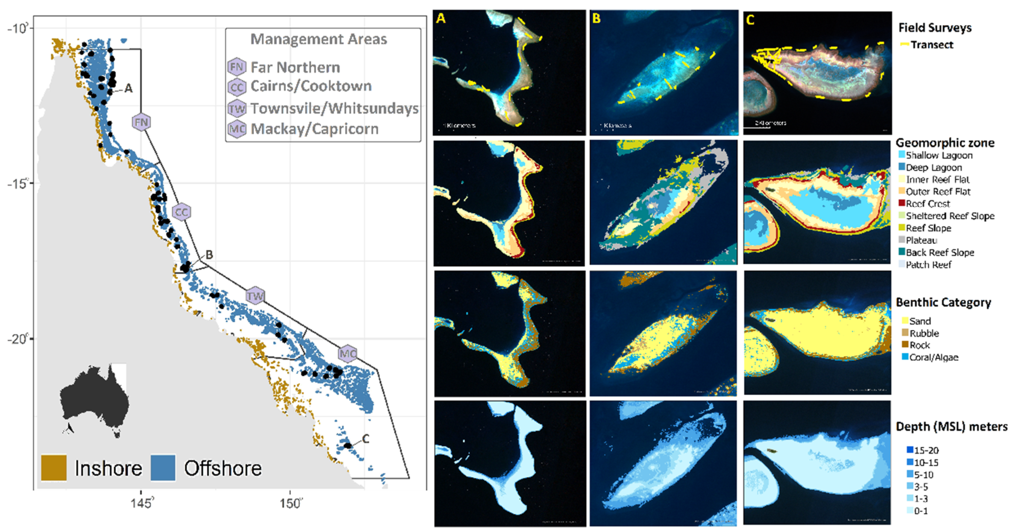
The study region includes approximately 2200 shallow offshore reefs within the Great Barrier Reef Marine Park (Figure 1). Here, the shallow offshore GBR includes all mid-shelf and outer reefs but excludes all nearshore fringing reefs as per References [40,52], because they are typically located in turbid waters and not visible from satellite imagery. Each of the mapped reefs was in clear water and visible to a depth of 20 m mean sea level (MSL), using optical Sentinel-2 satellite imagery (Figure 1).

Figure 1.
Shallow offshore GBR reefs (in blue) across GBRMPA management regions. Locations with field data (black dots) used for map calibration and validation. Sentinel-2 imagery of Wishbone Reef (A), Potter Reef (B) and Heron Reef (C) indicating the location of transects, geomorphic zonation map, benthic category map and derived depth (bathymetry). See Supplementary Materials Table S1 for definitions of mapping categories based on Reference [52].
2.2. Geomorphic Zonation and Benthic Category Maps
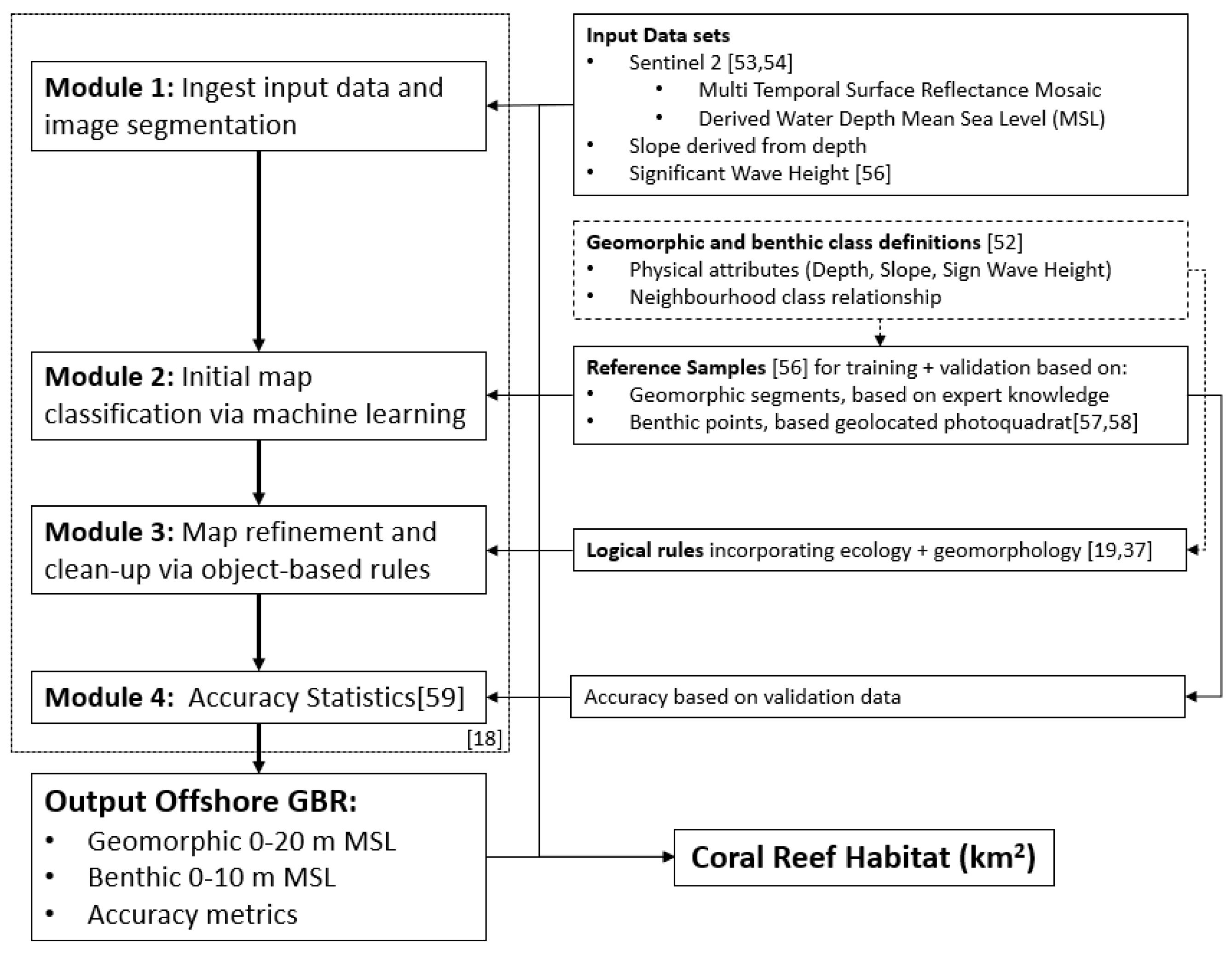
Geomorphic zonation (0–20 m MSL) and benthic category maps (0 m–10 m MSL), were generated via refinement of a previously developed mapping approach [18] successfully implemented on the GBR [19,38] (Figure 2). Habitat characterization followed a specific coral reef classification scheme where the ecology and geomorphology of each class was considered. This resulted in logical rules in relation to physical attributes (Depth, Slope, and Wave Height) and neighborhood relationships [52] that produced detailed geomorphic and benthic class definitions (Figure 2) (see short description in Supplementary Materials Table S1). To characterize benthic composition, the distribution of four benthic classes was considered: coral/algae, rock, rubble and sand [52].
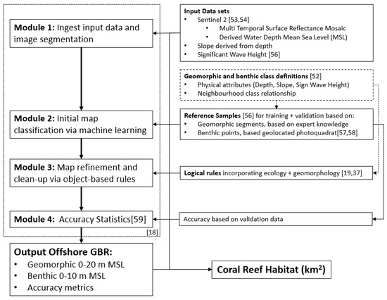
Figure 2.
Flowchart conceptualizing the four modules for mapping geomorphic and benthic categories with refinements for the shallow offshore Great Barrier Reefs, using specific input datasets. Framework adapted from Reference [18].
Refinements applied in this study include the use of precision corrected Sentinel-2 (10 m × 10 m) imagery, used as both the base visual image data and as the input for the various derived products (Figure 2). Here, Sentinel-2 scenes from May–October 2018 were used to create a cloud-free mosaic by assessing for multiple scenes for each position, and then calculate the bathymetry and reflectance data statistics for each pixel [53,54]. Sub-surface reflectance as well as tide-corrected depth (bathymetry) at MSL were calculated using the Modular Inversion and Processing (MIP) system that has been tested and validated worldwide [19,53,54]. This procedure improves the overall performance of the reflectance and bathymetry data. The latter was tidal corrected to MSL, using Admiralty Total Tide data of various stations along the coast of the GBR and compared with field depth measurements yielded an r2 of 0.85, n = 78,800, using a Garmin GPS echo sounder 550C. The satellite derived depth was then used to derive slope for each pixel using local gradient methods from a 3 × 3 moving window. Significant wave height was determined using numerical modeling of wave generation and propagation throughout the GBR, using a Simulating Waves Nearshore (SWAN) model, and near-reef transformations, using local wind data and Sentinel-2-derived depth [55].
Reference samples were acquired for calibration and validation of the geomorphic and benthic category maps. Geomorphic reference samples were manually created by experts [56] by assigning classes to selected segments guided by the geomorphic classification scheme [52], and following a traditional manual image interpretation technique (Figure 2). 26 reef areas were chosen for which satellite imagery was automatically segmented into image objects (groups of pixels) based on shape, color and texture. Segments were assigned a geomorphic class via interpretation of satellite imagery, depth, slope, wave intensity and spatial location within the reef. The benthic reference samples were derived from approximately 100,000 geolocated benthic photoquadrats [57] collected in January, May and December 2017; and April/May and December 2019, along 258 snorkel and 278 dive transects distributed over 78 reefs along the GBR (Figure 1). Benthic composition was derived from the photoquadrats via deep learning convolutional neural networks [58]. Approximately 3–5% of the photoquadrats were manually labelled and used to train a classifier which automatically annotated the remaining photoquadrats [58]. Reference samples [59,60] were split into independent calibration and validations sets, to inform the classification approach in this study and to calculate accuracy statistics respectively. Standard error matrix-based accuracy metrics (overall, user) were calculated using a non-parametric bootstrapping approach [61], where the estimate was the mean of the sampling distribution and the 95% confidence intervals were the 95th percentile around the median. The 95% confidence interval on the area estimates was also calculated using the bootstrapped interval (see Supplementary Materials Table S3).
Modules 1 to 4 (Figure 2) describe the procedures developed in Google Earth Engine to create the maps [18]. In short, Module 1 segments the image and creates a data stack, Module 2 applies a random forest machine learning routine to the data stack, Module 3 applies contextual editing using object-based logical rules driven by an established classification scheme, Module 4 calculates the accuracy statistics, such as overall, user and producer accuracy by following a standard approach, using validation reference samples as input [62].
2.3. Calculating Reef Extent
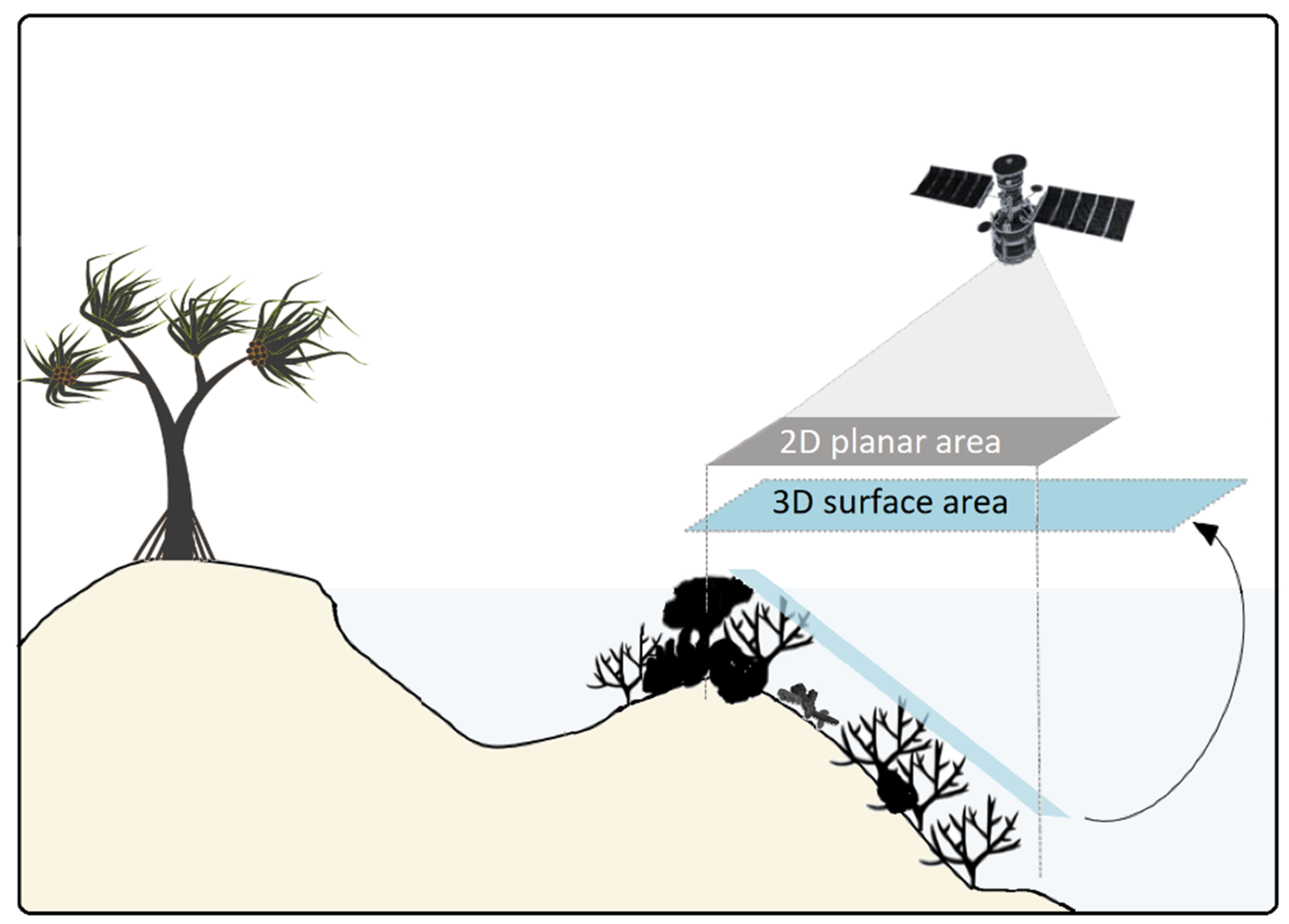
The 2D planar area (“birds-eye” map area) from the final habitat maps was converted to 3D surface area, using a “surface-to-horizontal-area ratio” derived from the slope value estimated for each pixel. Slope was estimated by using a local gradient method (3 × 3 window) from the tide-corrected depth estimates (Figure 1). The slope-adjusted surface area referred to as 3D surface area hereafter was calculated by using a trigonometric multiplication of 2D surface area and the slope (2D area/cos(slope)), where the slope is in radians (Figure 3).

Figure 3.
Conceptual diagram for calculation of 3D surface area based on 2D planar area (i.e., horizontal projected area) and the slope component. Example shown for the slope geomorphic zone. Graphics courtesy of the Integration and Application Network, University of Maryland Center for Environmental Science.
The 3D surface area was used to estimate reef extent and the extent of each benthic category and geomorphic zone. Extent was defined as the area representing the mapped feature, e.g., reef, benthic category or geomorphic zone. Data outputs are presented as summaries at the level of management areas of the GBR Marine Park, as defined by GBRMPA: Far North, Cairns/Cooktown, Townsville/Whitsunday, Mackay/Capricorn. Individual reef maps can be accessed and downloaded through GBRMPA Reef Knowledge System—Reef Explorer [63].
2.4. Calculating Coral Habitat
In order to estimate the amount of coral habitat on the GBR, we used the benthic category map (i.e., reef data down to a 10 m depth), as it represents the finest resolution of benthic data that allow differentiation of substrate types. It was assumed that a consolidated reef surface (i.e., hard substrate) could provide the structure suitable for coral settlement and growth [50]. Hence, the coral/algae and rock categories were denoted suitable substrates, whereas rubble and sand, which represent loose, unconsolidated substrates, were assumed inappropriate for coral growth. Data are summarized at 0.2 degree intervals to highlight distribution along the length of the GBR. A broader generalization of coral habitat (not detailed here for simplicity) may be derived from the geomorphic maps (reef data down to 20 m depth), assuming that hard substrate is the dominant substrate type on reef slope, outer reef flat and reef crest habitats (Supplementary Materials Figure S1).
3. Results
3.1. Geomorphic Zonation and Benthic Category Maps
The geomorphic zonation and benthic category maps created in this study [63] are the highest-resolution maps to date for the offshore GBR and were tailored to meet the specific scientific and management needs for the GBRMP that were not met by existing large scale mapping efforts [18]. Coral/algae was mapped as a single class, because it was not possible to differentiate between coral and algae, using the input data in this study. Coral and algae can typically only be separated by using hyperspectral sensors [64] and not multispectral sensors, such as the Sentinel-2 (this study) [36], and coral that is overgrown with photosynthetic algae has a similar spectral response to coral rubble or live coral [65]. Although we did not attempt to differentiate between coral and algae directly, our approach utilized multiple input data sources (i.e., texture, context, depth, slope and waves) and performed well for the separation of the four benthic classes (Supplementary Materials Table S2), as comparable to previous studies [38,66,67].
Overall map accuracies for the geomorphic and benthic maps were 68% and 62%, respectively (see Supplementary Materials Table S2 for full accuracy results). Estimates of the composition of broad benthic categories at the scale of individual reefs down to 10 m mean sea level (MSL) (1946 shallow offshore reefs) are provided on the benthic category maps. The geomorphic characterization of each reef, down to 20 m MSL (2164 reefs), is compiled in the geomorphic zonation maps [63].
3.2. Reef Extent
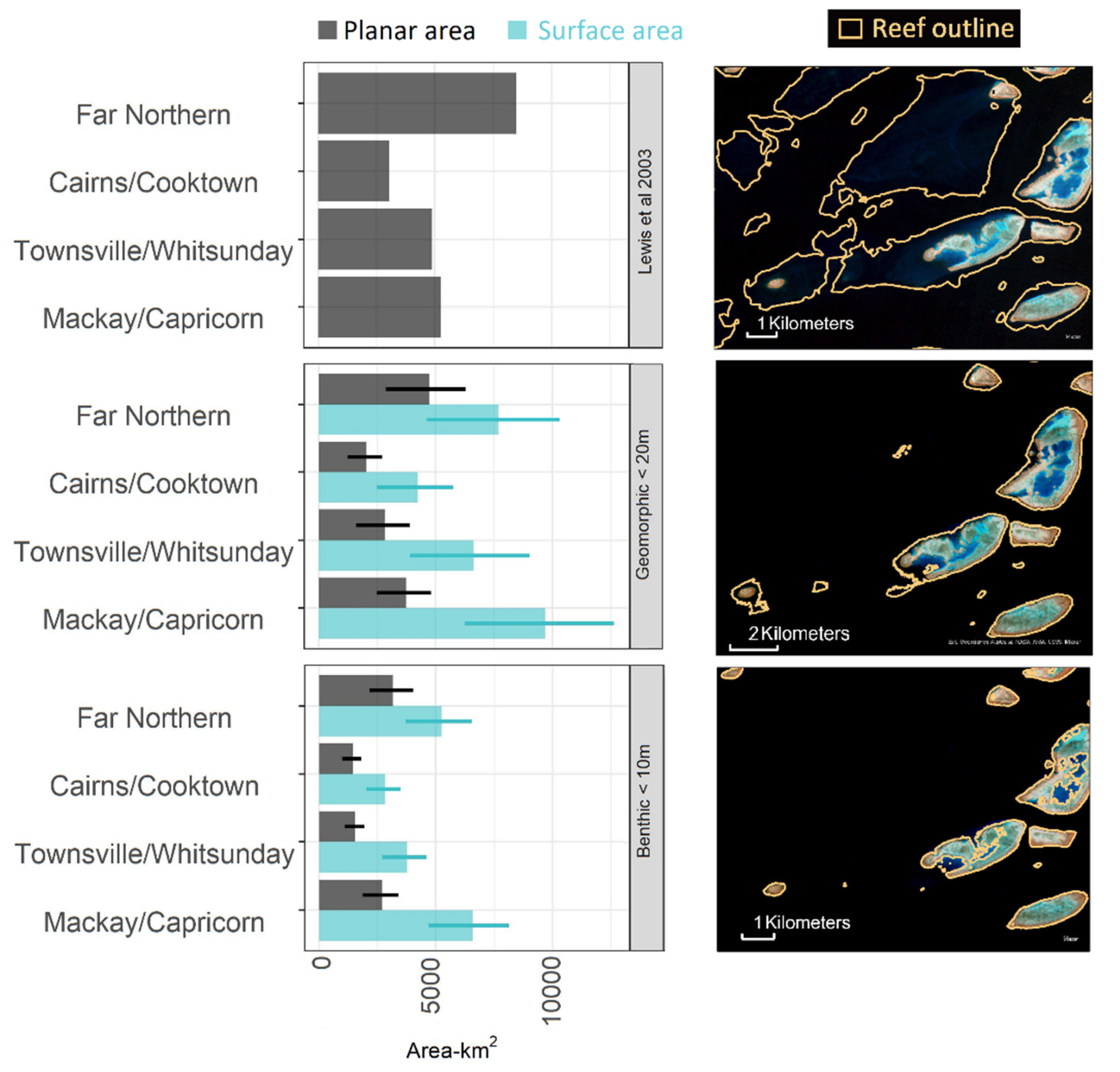
Our capacity to discriminate reef substrate types and to exclude areas of deep water (beyond 20 m depth) resulted in a 39% to 60% reduction of 2D planar area estimates (based on geomorphic and benthic maps respectively) compared to Lewis et al. [27] (Figure 4). New reef outlines derived from our new 2D maps provide better support for ecological studies by allowing for more accurate determination of reef size and distance between reefs, for example, information that, until now, has been derived from Lewis et al. [27] maps (see example of reef outlines in Figure 4).

Figure 4.
Comparison of 2D planar and 3D surface area (gray and blue bars, respectively) per region. Error bars denote 95% Confidence Intervals. Estimates based on reef outline provided by Lewis et al., 2003 [27] (top panel) compared to this study based on geomorphic zones above 20 m MSL (middle panel) and mapped benthic categories above 10 m MSL (bottom panel). Visualization of respective reef outlines based on mapped areas from the Mackay/Capricorn region overlaid on Sentinel 2 satellite imagery.
Based on the benthic category maps, we calculated 18,388 km2 (13,127–22,722 km2 95% Confidence Interval) of 3D surface area (shallow coral reef < 10 m). Mapping reefs to a depth of 20 m based on geomorphic zonation yielded a total 3D surface area of 28,261 km2 (17,267–37,716 km2 95% Confidence Interval) and provided information for an additional 218 reefs. Estimating the 3D surface area (i.e., by considering slope) increased estimates of mapped reef areas by up to a factor of 2.9 for reef-slope habitats (Supplementary Materials Table S3). Overall 3D estimates for the entire GBR increased by ~9552 km2 when compared to our own planar estimates (Figure 3). Similarly, we observed a 31% increase in 3D surface area compared to current 2D planar estimates, using the existing reef outline [27] for the same shallow offshore reef region. This increase of reef extent was driven predominantly by reefs of the Mackay/Capricorn management area in the Southern GBR (Figure 4).
3.3. Benthic Categories across the GBR
There is considerable variability in benthic composition among reefs [63], and this variability reflects the diversity of geomorphic zones across the GBR. For example, lagoon habitats, which are sand-dominated, were on average nearly two-fold larger on Far-North reefs compared to reefs in the Capricorn region (Supplementary Materials Table S3). At regional scales, mapped areas dominated by coral/algae (from ~24% in Cairns/Cooktown to ~33% in the Far North) and rock (from ~22% in the Far North to ~37% in Townsville/Whitsundays) were the most variable across regions, whereas little variability was found in the surface area mapped as rubble (from ~6% in Far North to ~9% in Cairns/Cooktown) and sand (from 30% in Townsville/Whitsundays to 38% in Far North) among management regions (Figure 5). However, at the reef level, areas mapped as rubble were, on average, 53–68% greater on the Central GBR (Cairn to Whitsundays region) compared to the Far-North and Southernmost regions (Supplementary Materials Table S3). Whether this estimate reflects localized past history of disturbance impacts from repeated cyclones and/or bleaching is out of the scope in this study but needs to be explored in more detail.
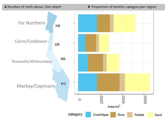
Figure 5.
(A) Total number of offshore reefs mapped above 10 m depth used for estimation of benthic category areas across management regions. (B) Surface area per benthic category (coral/algae, sand, rock and rubble) per region.
3.4. Coral Habitat
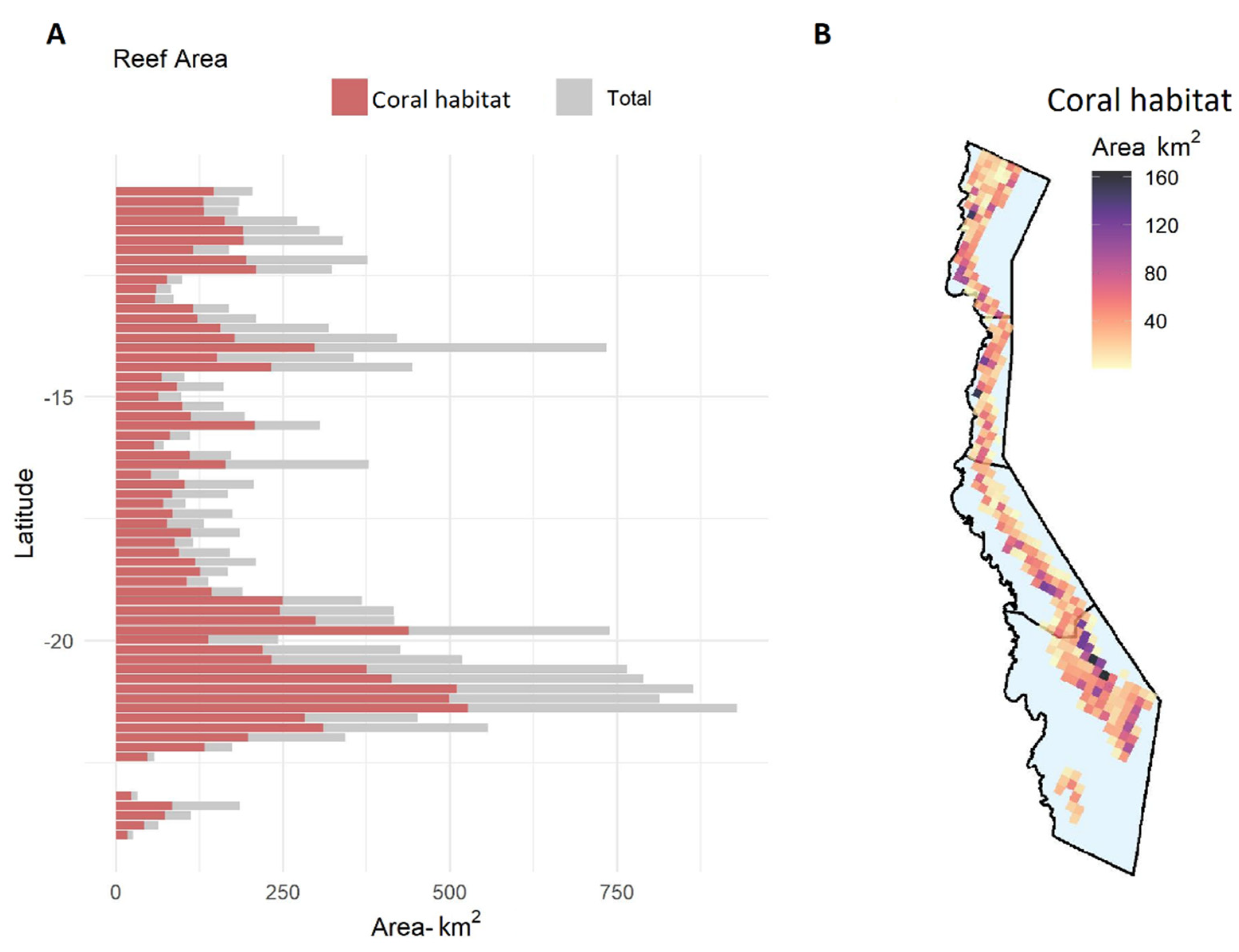
The area of hard consolidated substrates which are considered suitable coral habitat (i.e., excluding sand and rubble areas) was estimated at 10,613 km2 (8696–11,828 km2, 95% Confidence Interval) for the entire GBRMP based on benthic maps created for this study, with considerable variation along latitudinal (Figure 6A) and cross-shelf (Figure 6B) direction of the GBR. Overall, the southern reefs between −22 and −23 degrees latitude had the highest estimates of coral habitat (>500 km2 on average) concentrated in the outermost reefs. In contrast, the central region, specifically between Cairns and Townsville, had the lowest estimates of coral habitat (<100 km2 on average).
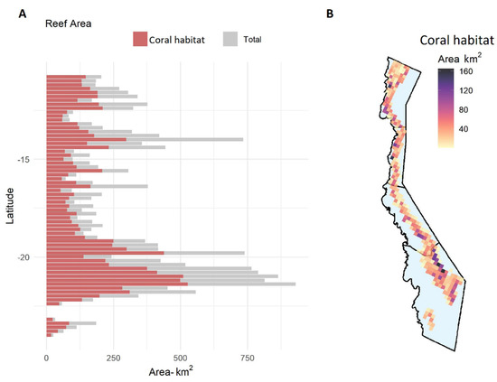
Figure 6.
(A) Latitudinal distribution of coral habitat (in red: a 3D surface area estimate of hard substrate potentially available for settlement and establishment of coral populations) as a proportion of total 3D surface area above 10 m MSL depth (in grey). Estimates derived from benthic category maps (i.e., area of coral/algae and rock vs. total 3D surface area). (B) Spatial distribution of coral habitat along and across the GBR (each pixel is a 0.2 × 0.2 degree cell).
4. Discussion
This study provides the first detailed description of the reef extent, benthic composition and coral habitat for each of the 1945 shallow offshore reefs of the Great Barrier Reef. These reefs characterize the shallow mid- and outer-shelf regions of the GBR which represent 51% of the entire GBRMP. A broader characterization down to 20 m MSL, based on geomorphic zones, was possible for 57% of the GBR (2164 reefs). Our new geomorphic and benthic habitat maps provide the highest level of spatial (10 m × 10 m) and thematic detail (12 geomorphic and four benthic classes) currently available for the GBR refining previous studies on reef extent for the same area [27,68]. Specifically, our coral habitat maps provide a solid baseline to inform management on the potential settlement and growing areas for coral communities and complement similar research performed for deeper GBR reefs [22].
Other large coral reef areas (>50 reefs covering >1000 km2) have been previously mapped by remote-sensing efforts at the benthic [17] and geomorphic [69] scale. The work presented here focused on the GBR applying a standardized methodological approach that can be replicated for consistently mapping large-scale regions. Compared to previous GBR habitat-mapping efforts [18], here we used detailed benthic training and validation data derived from over 100,000 photoquadrats, employed a higher level of satellite image preprocessing and incorporated more accurate environmental properties (absolute depth and wave height).
While an even higher level of thematic benthic detail could be achieved with higher-resolution imagery at 1–2 m pixels [17] and hyperspectral imagery [54,64], sensors capable of these properties are not yet available for consistent and regular large-area coverage (thousands of kilometers). Airborne high-spatial-resolution hyperspectral sensors [64,70] have been previously used for mapping these type of properties for relatively small (tens to hundreds of kilometers) reef areas. In the future, satellite sensors with improved spatial, temporal and spectral resolution are likely to provide enough coverage for mapping areas as large as the GBR. The general mapping workflow used in this study [18,52,56] is highly flexible and has been used on both large- and small-scale applications. It has been used on very high-resolution image data at the individual-reef scale [18,71], through to being applied to Planet Dove satellite imagery to map all reef systems globally [72]. Further improvement of the mapping would focus mostly on improving the input datasets. Although it is a generalizable workflow, we were fundamentally limited to how deep we could detect bottom types (i.e., <20 m) and by the thematic resolution at which we could differentiate them (i.e., we did not differentiate coral from algae). Improvements will also be realized from processes that increase the quality of the bottom signal in deep and turbid waters (e.g., some reefs are visible, but the reflectance values do not allow a classification in the current workflow). Our inability to differentiate coral and algae at large spatial scales is limiting some research and management applications, so further research is needed to assess other possibilities to estimate coral and algae separately.
Our new GBR habitat maps provide for the first time the opportunity to incorporate benthic composition and 3D reef characteristics in the calculation of reef extent and coral habitat area. These estimates, however, do not capture the steepest areas of the reefs (e.g., walls), as vertical areas cannot be mapped by using optical earth observation approaches, since virtually none of the benthos can be observed. Further analysis of sudden depth changes is needed to characterize steep walls, as this goes beyond the scope of the present study. It is unclear what depth cutoff was used to derive the reef outlines from previous GBR maps from which estimates of shallow reef extent ranged from 20,055 km2 [41] to 20,679 km2 [27] (Table 1). Limitations for mapping reefs from aerial photography or satellite imagery include detection limits due to depth, such that deeper reefs are missed. However, previous studies [22,73] that used a bathymetric model identified a further 25,600 km2 of submerged banks on the GBR between 20 and 200 m isobaths.

Table 1.
Comparison of available reef extent estimates for the Great Barrier Reef Marine Park (GBRMP). Confidence intervals (95% CI) are provided for this study.
The 3D surface area estimate is 31% greater than the estimates based on typical planar mapped area, and this demonstrates the importance of consideration of the three-dimensional nature of reefs in the production of habitat maps. It provides a closer quantitative representation of the real reef area that requires monitoring and management. The GBRMPA management regions vary in reef type and composition, which resulted in differences in reef extent. In particular, the Mackay/Capricorn region, albeit presenting the smallest average reef size, has a higher reef surface area relative to other management regions, resulting from the greater number of reefs (42% of mapped reefs) but also steeper reef slopes (Supplementary Materials Table S3).
Total coral cover is the most common indicator used to evaluate reef health [74], but only a few monitored reefs are used to infer coral cover at the scale of the entire GBR. Studies based on monitored reefs [24,47,75,76] provide detailed information on benthic community composition that is not captured here. However, extrapolations to scale the entire ecosystem are limited by the lack of characterization of reefs elsewhere. In this study, refined estimates of the total amount of area on the GBR available for coral settlement and growth may help interpolation of spatially discrete monitoring data into reefal and reef-system-wide estimates of total coral cover. Importantly, we used the same approach to map the entire GBR that provides the capability to study reefs individually, regionally or at the scale of the ecosystem. Specifically, benthic maps revealed the extent for coral/algae, rock, rubble and sand categories. Although this is a coarse characterization with four benthic classes, it provides the most complete and most spatially detailed description of reef-level benthic composition for the full length of the GBR. This information will refine ecosystem-based management tools [24,25,47] and improve predictions of coral cover based on the spatial extent of hard substrate.
The current study focuses on the mapping and spatial analysis of the shallow offshore reefs only, and future work should be directed to include the inshore reefs and reefs deeper than 20 m MSL. When calculating coral habitat, only substrate properties (i.e., consolidated hard substrate) were considered, but other biological, physical or ecological factors influence coral presence or growth. It is known, for instance, that available light influences coral distribution and growth [77]. Incorporating this type of information could further fine-tune estimates of coral habitat. In addition, we note that, by excluding areas dominated by unconsolidated substrate (e.g., lagoon areas), we may underestimate, in some regions, the total extent of coral habitat. There is some temporal mismatch between the satellite imagery (May–October 2018) and field data (January, May and December 2017; and April, May and December 2019) collected to produce the maps. Near-real-time observations (i.e., field-data collection coinciding with satellite image) is desirable for mapping the present reef conditions. This is especially important when wanting to capture large-scale coral mortality due to impacts from cyclones or massive bleaching, which could be detected with access to suitable hyperspectral airborne sensors. Most field observations and all satellite imagery were collected after any disturbance occurring between 2017 and 2019, e.g., mass bleaching event and the severe Tropical Cyclone Debbie in March 2017.
Management on the GBR relies heavily on science, and there is an ongoing effort in developing ecologically informed modeling approaches of coral dynamics for decision-making. We provide a novel tool with spatially explicit ecological information to characterize the GBR reef habitats at the highest spatial resolution available today. Our maps provide a better definition of reef-extent boundaries that can be coupled with existing environmental spatial layers and modeling approaches to improve management and decision-making for restoration practices.
Supplementary Materials
The following are available online at https://www.mdpi.com/article/10.3390/rs13214343/s1. Figure S1: Latitudinal distribution of reef area above 20 m MSL depth based on geomorphic zo-nation maps. (A) Latitudinal distribution of total reef area (grey) and coral habitat (green) above 20 m MSL depth based on geomorphic zonation maps. Coral habitat = area of Reef Slope, Reef Crest, and Outer Reef Flat. (B) Spatial distribution of coral habitat along and across the GBR (each pixel is a 0.2 × 0.2 degree cell). Table S1: Mapping category general description. Table S2: Error matrix. Table S3: Surface area for shallow offshore GBR.
Author Contributions
Conceptualization, C.M.R., M.B.L., C.C.-S., E.M.K., E.V.K. and S.R.P.; data curation, C.M.R., M.B.L., C.C.-S., E.M.K., D.C., M.W., K.M., P.T. and M.R.; formal analysis, C.M.R., M.B.L., C.C.-S., E.M.K., D.C., M.G.-R. and M.R.; funding acquisition, C.M.R. and S.R.P.; investigation, C.M.R., M.B.L., C.C.-S., E.M.K. and N.M.; methodology, C.M.R., M.B.L., C.C.-S., E.M.K., D.C., M.W. and N.M.; project administration, C.M.R.; resources, C.M.R., M.B.L., E.M.K. and M.W.; software, C.M.R. and M.B.L.; supervision, C.M.R.; validation, C.M.R., M.B.L., E.M.K., D.C., M.W., K.M., R.B.-A., M.R., E.V.K. and M.R.; visualization, M.G.-R., C.M.R., M.B.L. and C.C.-S.; writing—original draft, C.M.R., M.B.L., C.C.-S., E.M.K., E.V.K., N.M. and S.R.P.; writing—review and editing, C.M.R., M.B.L., C.C.-S., E.M.K., D.C., M.W., K.M., R.B.-A., E.V.K. and S.R.P. All authors have read and agreed to the published version of the manuscript.
Funding
This research was funded by Great Barrier Reef Marine Park Authority, Great Barrier Reef Foundation and Vulcan Philanthropy.
Institutional Review Board Statement
Not applicable.
Informed Consent Statement
Not applicable.
Data Availability Statement
The geomorphic zonation map, benthic composition map, satellite-derived bathymetry and surface-reflectance Sentinel-2 multi-temporal mosaic created in this study can be found and downloaded from the Great Barrier Reef Marine Park Authority Knowledge System Website [63], including previous reef extent layers. Reference samples used for training and validation are accessible through fig share for benthic [59] https://doi.org/10.6084/m9.figshare.14464764, accessed on 11 July 2021 and geomorphic [60] https://doi.org/10.6084/m9.figshare.14464755, accessed on 11 July 2021.
Acknowledgments
Field work was made possible by David Stewart and his team on MV Kalinda, The GBR Legacy Expedition, Ocean Mapping Expedition with MV Fleur du Passion and field teams Breanne Vincent, Peran Brea, Josh Passenger, Stefano Freguaria, Douglas Stetner, Monique Groll, Alex Ordonez, Karen Johnson, Karen Joyce and Stephanie Duce. Javier Leon and Monique Groll on the GBR Legacy December 2019 field trip. OBIA image analysis eCognition software support was provided by Trimble. Google Earth Engine supported by Google. The high-performance computing was supported by Queensland Cyber Infrastructure Foundation and The University of Queensland. We would also like to thank the anonymous reviewers their comments, which helped us to improve the manuscript substantially.
Conflicts of Interest
The authors declare no conflict of interest. The funders had no role in the design of the study; in the collection, analyses or interpretation of data; in the writing of the manuscript; or in the decision to publish the results.
References
- Hamylton, S.; Duce, S.; Vila-Concejo, A.; Roelfsema, C.M.; Phinn, S.R.; Carvalho, R.C.; Shaw, E.C.; Joyce, K.E. Estimating regional coral reef calcium carbonate production from remotely sensed seafloor maps. Remote Sens. Environ. 2017, 201, 88–98. [Google Scholar] [CrossRef]
- Brown, C.; Smith, S.J.; Lawton, P.; Anderson, J.T. Benthic habitat mapping: A review of progress towards improved understanding of the spatial ecology of the seafloor using acoustic techniques. Estuar. Coast. Shelf Sci. 2011, 92, 502–520. [Google Scholar] [CrossRef]
- Kostylev, V.E.; Todd, B.J.; Fader, G.B.J.; Courtney, R.C.; Cameron, G.D.M.; Pickrill, R.A. Benthic habitat mapping on the Scotian Shelf based on multibeam bathymetry, surficial geology and sea floor photographs. Mar. Ecol. Prog. Ser. 2001, 219, 121–137. [Google Scholar] [CrossRef] [Green Version]
- Lecours, V.; Devillers, R.; Schneider, D.C.; Lucieer, V.L.; Brown, C.; Edinger, E.N. Spatial scale and geographic context in benthic habitat mapping: Review and future directions. Mar. Ecol. Prog. Ser. 2015, 535, 259–284. [Google Scholar] [CrossRef] [Green Version]
- Brown, C.; Sameoto, J.A.; Smith, S.J. Multiple methods, maps, and management applications: Purpose made seafloor maps in support of ocean management. J. Sea Res. 2012, 72, 1–13. [Google Scholar] [CrossRef]
- Lee, C.K.; Nicholson, E.; Duncan, C.; Murray, N.J. Estimating changes and trends in ecosystem extent with dense time-series satellite remote sensing. Conserv. Biol. 2021, 35, 325–335. [Google Scholar] [CrossRef]
- Pandolfi, J.M.; Bradbury, R.H.; Sala, E.; Hughes, T.P.; Bjorndal, K.A.; Cooke, R.G.; McArdle, D.; McClenachan, L.; Newman, M.J.H.; Paredes, G.; et al. Global Trajectories of the Long-Term Decline of Coral Reef Ecosystems. Science 2003, 301, 955–958. [Google Scholar] [CrossRef] [Green Version]
- Hughes, T.P.; Kerry, J.T.; Baird, A.H.; Connolly, S.R.; Dietzel, A.; Eakin, C.M.; Heron, S.; Hoey, A.S.; Hoogenboom, M.O.; Liu, G.; et al. Global warming transforms coral reef assemblages. Nat. Cell Biol. 2018, 556, 492–496. [Google Scholar] [CrossRef]
- Knowlton, N.; Jackson, J.B.C. Shifting Baselines, Local Impacts, and Global Change on Coral Reefs. PLoS Biol. 2008, 6, e54. [Google Scholar] [CrossRef] [PubMed] [Green Version]
- Bellwood, D.R.; Pratchett, M.S.; Morrison, T.; Gurney, G.; Hughes, T.P.; Álvarez-Romero, J.; Day, J.C.; Grantham, R.; Grech, A.; Hoey, A.S.; et al. Coral reef conservation in the Anthropocene: Confronting spatial mismatches and prioritizing functions. Biol. Conserv. 2019, 236, 604–615. [Google Scholar] [CrossRef]
- Pittman, S.; Christensen, J.; Caldow, C.; Menza, C.; Monaco, M. Predictive mapping of fish species richness across shallow-water seascapes in the Caribbean. Ecol. Model. 2007, 204, 9–21. [Google Scholar] [CrossRef]
- Anthony, K.; Bay, L.K.; Costanza, R.; Firn, J.; Gunn, J.; Harrison, P.; Heyward, A.; Lundgren, P.; Mead, D.; Moore, T.; et al. New interventions are needed to save coral reefs. Nat. Ecol. Evol. 2017, 1, 1420–1422. [Google Scholar] [CrossRef]
- Hedley, J.D.; Roelfsema, C.M.; Chollett, I.; Harborne, A.R.; Heron, S.F.; Weeks, S.; Skirving, W.J.; Strong, A.E.; Eakin, C.M.; Christensen, T.R.L.; et al. Remote Sensing of Coral Reefs for Monitoring and Management: A Review. Remote Sens. 2016, 8, 118. [Google Scholar] [CrossRef] [Green Version]
- Andréfouët, S.; Riegl, B. Remote sensing: A key tool for interdisciplinary assessment of coral reef processes. Coral Reefs 2004, 23, 1–4. [Google Scholar] [CrossRef]
- Andréfouët, S. Coral reef habitat mapping using remote sensing: A user vs producer perspective. implications for research, management and capacity building. J. Spat. Sci. 2008, 53, 113–129. [Google Scholar] [CrossRef]
- Goodman, J.; Purkis, S.; Phinn, S.R. (Eds.) Coral Reef Remote Sensing: A Guide for Multi-Level Sensing Mapping and Assessment; Springer: Berlin, Germany, 2013. [Google Scholar]
- Purkis, S.J.; Gleason, A.C.R.; Purkis, C.R.; Dempsey, A.C.; Renaud, P.G.; Faisal, M.; Saul, S.; Kerr, J.M. High-resolution habitat and bathymetry maps for 65,000 sq. km of Earth’s remotest coral reefs. Coral Reefs 2019, 38, 467–488. [Google Scholar] [CrossRef] [Green Version]
- Lyons, M.; Roelfsema, C.; Kennedy, E.; Kovacs, E.; Borrego, R.; Markey, K.; Roe, M.; Yuwono, D.; Harris, D.; Phinn, S.; et al. Mapping the world’s coral reefs using a global multiscale earth observation framework. Remote Sens. Ecol. Conserv. 2020, 6, 557–568. [Google Scholar] [CrossRef] [Green Version]
- Roelfsema, C.M.; Kovacs, E.M.; Ortiz, J.C.; Callaghan, D.P.; Hock, K.; Mongin, M.; Johansen, K.; Mumby, P.J.; Wettle, M.; Ronan, M.; et al. Habitat maps to enhance monitoring and management of the Great Barrier Reef. Coral Reefs 2020, 39, 1039–1054. [Google Scholar] [CrossRef]
- Miller, I.R.; Jonker, M.J.; Osborne, K. Scuba search technique: Surveys of agents of coral mortality. In Long-Term Monitoring of the Great Barrier Reef-Standard Operational Procedure Number 8; Australian Institute of Marine Science: Townsville, Australia, 2020; p. 30. [Google Scholar]
- AIMS. Australian Institute of Marine Science Reef Monitoring. 2021. Available online: https://apps.aims.gov.au/reef-monitoring/ (accessed on 18 June 2021).
- Harris, P.T.; Bridge, T.C.; Beaman, R.J.; Webster, J.M.; Nichol, S.L.; Brooke, B.P. Submerged banks in the Great Barrier Reef, Australia, greatly increase available coral reef habitat. ICES J. Mar. Sci. 2013, 70, 284–293. [Google Scholar] [CrossRef] [Green Version]
- Bridge, T.; Beaman, R.; Done, T.; Webster, J. Predicting the Location and Spatial Extent of Submerged Coral Reef Habitat in the Great Barrier Reef World Heritage Area, Australia. PLoS ONE 2012, 7, e48203. [Google Scholar] [CrossRef] [Green Version]
- Bozec, Y.-M.; Hock, K.; Mason, R.A.B.; Baird, M.E.; Castro-Sanguino, C.; Condie, S.A.; Puotinen, M.; Thompson, A.; Mumby, P.J. Cumulative Impacts across Australia’s Great Barrier Reef: A Mechanistic Evaluation. 2020. Available online: https://www.biorxiv.org/content/10.1101/2020.12.01.406413v1 (accessed on 28 October 2021).
- Condie, S.A.; Anthony, K.R.N.; Babcock, R.C.; Baird, M.E.; Beeden, R.; Fletcher, C.S.; Gorton, R.; Harrison, D.; Hobday, A.J.; Plagányi, É.E.; et al. Large-scale interventions may delay decline of the Great Barrier Reef. R. Soc. Open Sci. 2021, 8, 201296. [Google Scholar] [CrossRef]
- Jupp, D.L.; Mayo, K.K.; Kuchler, D.A.; Claasen, D.V.R.; Kenchington, R.A.; Guerin, P.R. Remote sensing for planning and managing the great barrier reef of Australia. Photogrammetria 1985, 40, 21–42. [Google Scholar] [CrossRef]
- Lewis, A.; Lowe, D.; Otto, J. Remapping the Great Barrier Reef in Position Magazine; South pacific Science Press International: Alexandria, Australia, 2003; pp. 46–49. [Google Scholar]
- Neil, D.T.; Phinn, S.R.; Ahmad, W. Reef zonation and cover mapping with Landsat Thematic Mapper data: Intraand inter-reef patterns in the southern Great Barrier Reef region. In Proceedings of the IGARSS 2000. IEEE 2000 International Geoscience and Remote Sensing Symposium, Taking the Pulse of the Planet: The Role of Remote Sensing in Managing the Environment, Honolulu, HI, USA, 24–28 July 2000; IEEE: Piscataway, NJ, USA, 2002; Volume 5, pp. 1886–1888. [Google Scholar]
- Leon, J.; Woodroffe, C. Improving the synoptic mapping of coral reef geomorphology using object-based image analysis. Int. J. Geogr. Inf. Sci. 2011, 25, 949–969. [Google Scholar] [CrossRef]
- Joyce, K.E.; Phinn, S.R.; Roelfsema, C.M.; Neil, D.T.; Dennison, W.C. Combining Landsat ETM plus and Reef Check classifications for mapping coral reefs: A critical assessment from the southern Great Barrier Reef, Australia. Coral Reefs 2004, 23, 21–25. [Google Scholar] [CrossRef]
- Hamylton, S.; Carvalho, R.C.; Duce, S.; Roelfsema, C.M.; Vila-Concejo, A. Linking pattern to process in reef sediment dynamics at Lady Musgrave Island, southern Great Barrier Reef. Sedimentology 2016, 63, 1634–1650. [Google Scholar] [CrossRef] [Green Version]
- Kutser, T.; Parslow, J.; Clementson, L.; Skirving, W.; Done, T.J.; Wakeford, M.; Miller, I. Hyperspectral detection of coral reef bottom types. In Proceedings of the Ocean Optics XV, Adelaide, Australia, 21–25 August 2000. [Google Scholar]
- Hamylton, S. Will Coral Islands Maintain Their Growth over the Next Century? A Deterministic Model of Sediment Availability at Lady Elliot Island, Great Barrier Reef. PLoS ONE 2014, 9, e94067. [Google Scholar] [CrossRef] [PubMed] [Green Version]
- Andréfouët, S.; Berkelmans, R.; Odriozola, L.; Done, T.; Oliver, J.; Müller-Karger, F. Choosing the appropriate spatial resolution for monitoring coral bleaching events using remote sensing. Coral Reefs 2002, 21, 147–154. [Google Scholar] [CrossRef]
- Elvidge, C.D.; Dietz, J.B.; Berkelmans, R.; Andréfouët, S.; Skirving, W.; Strong, A.E.; Tuttle, B.T. Satellite observation of Keppel Islands (Great Barrier Reef) 2002 coral bleaching using IKONOS data. Coral Reefs 2004, 23, 123–132. [Google Scholar] [CrossRef]
- Hedley, J.D.; Roelfsema, C.; Brando, V.; Giardino, C.; Kutser, T.; Phinn, S.; Mumby, P.; Barrilero, O.; Laporte, J.; Koetz, B. Coral reef applications of Sentinel-2: Coverage, characteristics, bathymetry and benthic mapping with comparison to Landsat 8. Remote Sens. Environ. 2018, 216, 598–614. [Google Scholar] [CrossRef]
- Phinn, S.R.; Roelfsema, C.M.; Mumby, P.J. Benthic cover map of Heron Reef derived from a high-spatial-resolution multi-spectra Multi-scale, object-based image analysis for mapping geomorphic and ecological zones on coral reefs. Int. J. Remote Sens. 2012, 33, 768–3797. [Google Scholar] [CrossRef]
- Roelfsema, C.; Kovacs, E.; Ortiz, J.C.; Wolff, N.; Callaghan, D.; Wettle, M.; Ronan, M.; Hamylton, S.; Mumby, P.; Phinn, S. Coral reef habitat mapping: A combination of object-based image analysis and ecological modelling. Remote Sens. Environ. 2018, 208, 27–41. [Google Scholar] [CrossRef]
- Roelfsema, C.; Kovacs, E.; Roos, P.; Terzano, D.; Lyons, M.; Phinn, S. Use of a semi-automated object based analysis to map benthic composition, Heron Reef, Southern Great Barrier Reef. Remote Sens. Lett. 2018, 9, 324–333. [Google Scholar] [CrossRef]
- Kerrigan, B.; Breen, D.; Death, G.; Day, J.; Fernandes, L.; Tobin, R.; Dobbs, K. Classifying the Biodiversity of the Great Barrier Reef World Heritage Area. In Great Barrier Reef Marine Park Authorithy; Australia, C.O., Ed.; Research Publication: Townsville, Australia, 2010; p. 55. [Google Scholar]
- Hopley, D.; Parnell, K.E.; Isdale, P.J. The Great Barrier Reef Marine Park: Dimensions and Regional Patterns. Aust. Geogr. Stud. 1989, 27, 47–66. [Google Scholar] [CrossRef]
- GBRMPA. Great Barrier Reef (GBR) Features (Reef Boundaries, QLD Mainland, Islands, Cays and Rocks; GBRMPA: Townsville, Australia, 2013.
- Baird, M.; Cherukuru, N.; Jones, E.; Margvelashvili, N.; Mongin, M.; Oubelkheir, K.; Ralph, P.; Rizwi, F.; Robson, B.; Schroeder, T.; et al. Remote-sensing reflectance and true colour produced by a coupled hydrodynamic, optical, sediment, biogeochemical model of the Great Barrier Reef, Australia: Comparison with satellite data. Environ. Model. Softw. 2016, 78, 79–96. [Google Scholar] [CrossRef]
- Baird, M.E.; Mongin, M.; Rizwi, F.; Bay, L.K.; Cantin, N.E.; Soja-Woźniak, M.; Skerratt, J. A mechanistic model of coral bleaching due to temperature-mediated light-driven reactive oxygen build-up in zooxanthellae. Ecol. Model. 2018, 386, 20–37. [Google Scholar] [CrossRef]
- Hock, K.; Wolff, N.H.; Condie, S.A.; Anthony, K.R.N.; Mumby, P.J. Connectivity networks reveal the risks of crown-of-thorns starfish outbreaks on the Great Barrier Reef. J. Appl. Ecol. 2014, 51, 1188–1196. [Google Scholar] [CrossRef] [Green Version]
- Matthews, S.; Shoemaker, K.; Pratchett, M.S.; Mellin, C. COTSMod: A spatially explicit metacommunity model of outbreaks of crown-of-thorns starfish and coral recovery. Adv. Mar. Biol. 2020, 87, 259–290. [Google Scholar] [PubMed]
- Mellin, C.; Matthews, S.; Anthony, K.R.; Brown, S.; Caley, M.J.; Johns, K.A.; Osborne, K.; Puotinen, M.; Thompson, A.; Wolff, N.H.; et al. Spatial resilience of the Great Barrier Reef under cumulative disturbance impacts. Glob. Chang. Biol. 2019, 25, 2431–2445. [Google Scholar] [CrossRef] [PubMed]
- Fletcher, C.S.; Castro-Sanguino, C.; Condie, S.; Bozec, Y.; Hock, K.; Gladish, D.W.; Mumby, P.J.; Westcott, D.A. Regional-Scale Modelling Capability for Assessing Crown-of-Thorns Starfish Control. Strategies on the Great Barrier Reef; Australian Government’s National Environmental Science Program: Cairns, Australia, 2021; p. 59.
- Hock, K.; Wolff, N.; Ortiz, J.C.; Condie, S.A.; Anthony, K.; Blackwell, P.G.; Mumby, P.J. Connectivity and systemic resilience of the Great Barrier Reef. PLoS Biol. 2017, 15, e2003355. [Google Scholar] [CrossRef]
- Madin, J.S.; Madin, E.M.P. The full extent of the global coral reef crisis. Conserv. Biol. 2015, 29, 1724–1726. [Google Scholar] [CrossRef] [PubMed]
- Kleypas, J.A.; McManus, J.W.; Meñez, L.A.B. Environmental Limits to Coral Reef Development: Where Do We Draw the Line? Am. Zool. 1999, 39, 146–159. [Google Scholar] [CrossRef]
- Kennedy, E.; Roelfsema, C.M.; Lyons, M.B.; Kovacs, E.; Borrego-Acevedo, R.; Roe, M.; Phinn, S.R.; Larsen, K.; Murray, N.; Yuwono, D.; et al. Reef Cover, a coral reef classification for global habitat mapping from remote sensing. Sci. Data 2021, 8, 1–20. [Google Scholar]
- Heege, T.; Bogner, A.; Pinnel, N. Mapping of submerged aquatic vegetation with a physically based process chain. In Remote Sensing of the Ocean and Sea Ice 2003; Bostater, C.R., Santoleri, R., Eds.; SPIE: Bellingham, WA, USA, 2004; pp. 43–50. [Google Scholar]
- Kobryn, H.T.; Wouters, K.; Beckley, L.E.; Heege, T. Ningaloo Reef: Shallow Marine Habitats Mapped Using a Hyperspectral Sensor. PLoS ONE 2013, 8, e70105. [Google Scholar] [CrossRef] [Green Version]
- Callaghan, D.P.; Leon, J.X.; Saunders, M.I. Wave modelling as a proxy for seagrass ecological modelling: Comparing fetch and process-based predictions for a bay and reef lagoon. Estuar. Coast. Shelf Sci. 2015, 153, 108–120. [Google Scholar] [CrossRef]
- Roelfsema, C.M.; Lyons, M.; Murray, N.; Kovacs, E.M.; Kennedy, E.; Markey, K.; Borrego-Acevedo, R.; Ordoñez Alvarez, A.; Say, C.; Tudman, P.; et al. Workflow for the Generation of Expert-Derived Training and Validation Data: A View to Global Scale Habitat Mapping. Front. Mar. Sci. 2021, 8, 228. [Google Scholar] [CrossRef]
- Roelfsema, C.M.; Phinn, S.R. Integrating field data with high spatial resolution multispectral satellite imagery for calibration and validation of coral reef benthic community maps. J. Appl. Remote Sens. 2010, 4, 1–28. [Google Scholar] [CrossRef] [Green Version]
- González-Rivero, M.; Beijbom, O.; Rodriguez-Ramirez, A.; Holtrop, T.; González-Marrero, Y.; Ganase, A.; Roelfsema, C.; Phinn, S.; Hoegh-Guldberg, O. Scaling up Ecological Measurements of Coral Reefs Using Semi-Automated Field Image Collection and Analysis. Remote Sens. 2016, 8, 30. [Google Scholar] [CrossRef] [Green Version]
- Lyons, M.; Kovacs, E.; Borrego-Acevedo, R.; Canto, R.; Harris, D.; Kennedy, E.V.; Markey, K.; Murray, N.; Ordoñez Alvarez, A.; Roe, M.; et al. GBR and Torres Straight Benthic Type Reference Sample. 2021. Available online: https://doi.org/10.6084/m9.figshare.1446476428/10/2021 (accessed on 11 July 2021). [CrossRef]
- Lyons, M.; Kovacs, E.; Borrego-Acevedo, R.; Canto, R.; Harris, D.; Kennedy, E.V.; Markey, K.; Murray, N.; Ordoñez Alvarez, A.; Roe, M.; et al. GBR and Torres Straight Geomorphic Type Reference Sample. 2021. Available online: https://doi.org/10.6084/m9.figshare.1446475528/10/2021 (accessed on 11 July 2021). [CrossRef]
- Lyons, M.B.; Keith, D.A.; Phinn, S.R.; Mason, T.J.; Elith, J. A comparison of resampling methods for remote sensing classification and accuracy assessment. Remote Sens. Environ. 2018, 208, 145–153. [Google Scholar] [CrossRef]
- Congalton, R.G.; Green, K. Assessing the Accuracy of Remotely Sensed Data: Principles and Practices; Lewis Publishers: Boca Rotan, FL, USA, 1999; p. 137. [Google Scholar]
- GBRMPA. Reef Knowledge System-Interactive Map: Geomorphic and Benthic. 2021. Available online: https://reefiq.gbrmpa.gov.au/ReefKnowledgeSystem/Reef-tools/Interactive-maps/ReefExplorer (accessed on 20 June 2021).
- Hochberg, E.J.; Atkinson, M.J. Capabilities of remote sensors to classify coral, algae, and sand as pure and mixed spectra. Remote Sens. Environ. 2003, 85, 174–189. [Google Scholar] [CrossRef]
- Nurjannah, N.; Teruhisa, K.; Hiroya, Y.; Gulam, A.; Chair, R.; AS, M.A. Spectral response of the coral rubble, living corals, and dead corals: Study case on the Spermonde Archipelago, Indonesia. In Remote Sensing of the Marine Environment II; SPIE: Bellingham, WA, USA, 2012; Volume 8525, p. 85251A. [Google Scholar]
- Benfield, S.L.; Guzman, H.M.; Mair, J.M.; Young, J.A.T. Mapping the distribution of coral reefs and associated sublittoral habitats in Pacific Panama: A comparison of optical satellite sensors and classification methodologies. Int. J. Remote Sens. 2007, 28, 5047–5070. [Google Scholar] [CrossRef]
- Phinn, S.R.; Roelfsema, C.M.; Mumby, P.J. Multi-scale image segmentation for mapping coral reef geomorphic and benthic community zone. Int. J. Remote Sens. 2012, 33, 3768–3797. [Google Scholar] [CrossRef]
- Hopley, D. The Geomorphology of the Great Barrier Reef: Quaternary Development of Coral Reefs; John Wiley & Sons: Brisbane, Australia, 1982; p. 453. [Google Scholar]
- Andréfouët, S. Keynote Address: The Diversity and Extent of Planet Earth’s Modern Coral Reefs as View from Space. In International Coral Reef Symposium; ICRS: Okinawa, Japan, 2004. [Google Scholar]
- Foo, S.; Asner, G.P. Scaling Up Coral Reef Restoration Using Remote Sensing Technology. Front. Mar. Sci. 2019, 6, 79. [Google Scholar] [CrossRef] [Green Version]
- Kovacs, E.; Roelfsema, C.; Lyons, M.; Zhao, S.; Phinn, S. Seagrass habitat mapping: How do Landsat 8 OLI, Sentinel-2, ZY-3A, and Worldview-3 perform? Remote Sens. Lett. 2018, 9, 686–695. [Google Scholar] [CrossRef]
- Atlas, A.C. Imagery, Maps and Monitoring of the World’s Tropical Coral Reefs; Zenodo: Genève, Switzerland, 2020. [Google Scholar]
- Beaman, R.J. Project 3D-GBR: A High-Resolution Depth Model for the Great Barrier Reef and Coral Sea, in Final Report; MTSRF: Cairns, Australia, 2010. [Google Scholar]
- Obura, D.O.; Aeby, G.; Amornthammarong, N.; Appeltans, W.; Bax, N.; Bishop, J.; Brainard, R.E.; Chan, S.; Fletcher, P.; Gordon, T.A.C.; et al. Coral Reef Monitoring, Reef Assessment Technologies, and Ecosystem-Based Management. Front. Mar. Sci. 2019, 6, 580. [Google Scholar] [CrossRef] [Green Version]
- Castro-Sanguino, C.; Ortiz, J.C.; Thompson, A.; Wolff, N.H.; Ferrari, R.; Robson, B.; Magno-Canto, M.M.; Puotinen, M.; Fabricius, K.E.; Uthicke, S. Reef state and performance as indicators of cumulative impacts on coral reefs. Ecol. Indic. 2021, 123, 107335. [Google Scholar] [CrossRef]
- Sweatman, H.; Delean, S.; Syms, C. Assessing loss of coral cover on Australia’s Great Barrier Reef over two decades, with implications for longer-term trends. Coral Reefs 2011, 30, 521–531. [Google Scholar] [CrossRef]
- Tamir, R.; Eyal, G.; Kramer, N.; Laverick, J.H.; Loya, Y. Light environment drives the shallow-to-mesophotic coral community transition. Ecosphere 2019, 10, e02839. [Google Scholar] [CrossRef] [Green Version]

Publisher’s Note: MDPI stays neutral with regard to jurisdictional claims in published maps and institutional affiliations. |
© 2021 by the authors. Licensee MDPI, Basel, Switzerland. This article is an open access article distributed under the terms and conditions of the Creative Commons Attribution (CC BY) license (https://creativecommons.org/licenses/by/4.0/).