Article

Potential Contributors to Common Mode Error in Array GPS Displacement Fields in Taiwan Island

1
Engineering Laboratory of Spatial Information Technology of Highway Geological Disaster Early Warning in Hunan Province, Changsha University of Science & Technology, Changsha 410114, China
2
School of Traffic and Transportation Engineering, Changsha University of Science & Technology, Changsha 410114, China
3
School of Geosciences and Info-Physics, Central South University, Changsha 410012, China
*
Author to whom correspondence should be addressed.
Remote Sens. 2021, 13(21), 4221; https://doi.org/10.3390/rs13214221
Submission received: 19 September 2021 / Revised: 19 October 2021 / Accepted: 19 October 2021 / Published: 21 October 2021
(This article belongs to the Special Issue BDS/GNSS for Earth Observation)

Abstract

:
The existence of the common mode error (CME) in the continuous global navigation satellite system (GNSS) coordinate time series affects geophysical studies that use GNSS observations. To understand the potential contributors of CME in GNSS networks in Taiwan and their effect on velocity estimations, we used the principal component analysis (PCA) and independent component analysis (ICA) to filter the vertical coordinate time series from 44 high-quality GNSS stations in Taiwan island in China, with a span of 10 years. The filtering effects have been evaluated and the potential causes of the CME are analyzed. The root-mean-square values decreased by approximately 14% and 17% after spatio-temporal filtering using PCA and ICA, respectively. We then discuss the relationship between the CME sources obtained by ICA and the environmental loads. The results reveal that the independent displacements extracted by ICA correlate with the atmospheric mass loading (ATML) and land water storage mass loading (LWS) of Taiwan in terms of both its amplitude and phase. We then use the white noise plus power law noise model to quantitatively estimate the noise characteristics of the pre- and post-filtered coordinate time series based on the maximum likelihood estimation criterion. The results indicate that spatio-temporal filtering reduces the amplitude of the PL and the periodic terms in the GPS time series.

1. Introduction

Continuous global navigation satellite system (GNSS) networks have been widely used in the fields of geodesy and geophysics. The permanently operating ground reference stations provide not only a millimeter-level 3-D coordinate time series under a global reference frame, but also provide important observational data and quantitative constraints for studies involving crustal deformation and dynamic processes on a global and regional scale [1,2]. However, the GNSS data processing procedure is affected by many factors, and numerous errors occur in the GNSS terminal products [3,4,5]. Geophysical signals can be difficult to separate from noise and unknown error sources because they are hidden in a detrended residual coordinate time series. Previous studies have identified that a spatially correlated error generally exists in regional networks, caused by the reference frame, satellites orbits, ocean tide correction models, and other unknown errors. This is usually referred to as the common mode error (CME) [6,7,8,9,10,11]. The presence of this error affects the accuracy of the station coordinates and velocity solutions, and conceals many weak and transient signals in a coordinate time series (e.g., deep magma motion, fault motion).
Spatial filtering techniques can be used to mitigate the CME. There are presently two types of spatial filtering techniques, stacking [6,12] and empirical orthogonal function (EOF) decomposition [7], which have been widely used in the field of geodesy to detect transient signals. Wdowinski et al. [6] initially introduced stacking to detect co-seismic displacements in a residual position time series. However, Nikolaidis et al. [12] illustrated that stacking works satisfactorily when the CME in a regional network is essentially spatially homogeneous. Larger areas and weaker spatial correlations generally result in differences between the spatial response of the different stations to the CME. Previous studies have illustrated that the CME spatial correlation decreases with increasing distance and reaches 95% within 1000 km. For networks that exceed 2000 km, the CMEs exhibit significant differences in various regions and the spatial correlation is essentially nonexistent beyond 6000 km [13,14]. To address this problem, Tian et al. [15] proposed a correlation weighting stacking scheme. However, this algorithm is still affected by local-scale or site-specific changes, and further research is necessary to obtain the appropriate weights of all the sites at each epoch.
In comparison, Dong et al. [7] and Serpelloni et al. [16] verified that the EOF can decompose residual coordinate time series into different modes to extract the CME, which provides a stricter mathematical framework than stacking. Principal component analysis (PCA) does not require CME spatial uniformity, but adopts a uniform temporal function that affects stations across a regional network. Dong et al. [7] reviewed the spatial consistency of stations using a visual appraisal of the decomposed principal components (PCs) to extract the CME from the Southern California Integrated GPS Network (SCIGN). PCA and its extensions have been subsequently used to eliminate the CME in local area networks [8,17,18,19,20,21,22,23,24].
Previous studies focused on the effective removal of CME from a GNSS coordinate time series to improve the accuracy of coordinate solutions from regional network measurements [25], which is conducive to the study of some geophysical applications using GNSS, such as the assessment of glacial isostatic adjustment models [26] and crustal movement [27,28]. Other studies have addressed the potential contributors of CME, particularly the potential geophysical signals [18,21,29,30,31,32,33,34,35,36,37,38]. This is particularly relevant for crustal deformation caused by the redistribution of surface mass, such as strongly seasonal water movements and atmospheric pressure changes. Kumar et al. [39] extracted the CME of Taiwan using the EOF, and quantitatively analyzed the CME in the U direction and atmospheric mass loading (ATML) of Taiwan, as calculated by the International Mass Loading Service (IMLS). They found a significantly high correlation and degree of concordance between the CME and ATML residuals for the vertical component. A further regression analysis revealed that the highest 90% of the non-seasonal ATML displacements in Taiwan are present in the CME variations.
However, the extraction of the CME using PCA still experiences some limitations for geophysical interpretation. PCA is based on the second-order statistics of variance and covariance, and therefore does not make full use of the higher-order CME statistics. PCA can work effectively in cases where there is only a single source in the CME. However, when the CME contains multiple competing sources, a single principal component (PC) may contain a mixture of contributions from different sources, which can easily generate artificial features. In contrast, Liu et al. [18,19,26], Ming et al. [38], and Yan et al. [29] applied an independent component analysis (ICA) to geodetic data sets and successfully separated seasonal and long-term trend signals.
Previous studies indicated the effectiveness of ICA in studying the potential contributors of CME in a regional GNSS coordinate time series. Thus, following the work of Kumar et al. [39], we apply a combination of PCA and ICA to the vertical coordinate time series of 44 stations from Taiwan island in China, and extract the CMEs of this network. The associated effects on the stations’ coordinate residuals and observed values are analyzed and compared. We discuss the relationship between the CME sources and environmental loadings, and compare GPS CMEs with vertical surface displacement predictions from the IMLS. We determine the cause of the Taiwan GNSS network CME, except for the atmosphere pressure loading (ATML), and separate the signals related to land water storage mass loading (LWS). The results further validate the accuracy of ICA applications for CME signal separation and the geophysical interpretation of regional networks. Changes in the optimal noise model of the GNSS stations before and after the ICA filtering are analyzed, as well as the differences between the time series parameters of the GNSS stations.

2. Methods and Data Processing

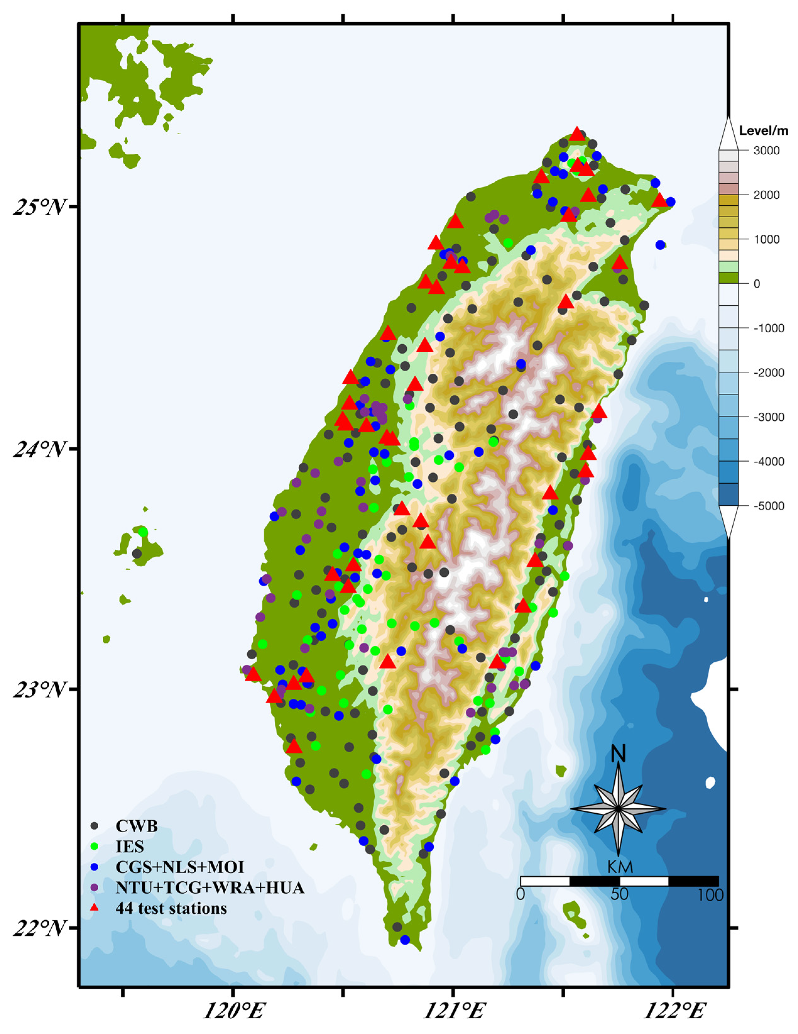
2.1. GNSS Data Processing

All of the stations in Taiwan’s continuous GPS (CGPS) array are equipped with dual-frequency geodetic GNSS receivers (Trimble 4000 SST Geodetic II P and 4000 SSE/SSIGeodetic Surveyor) [40]. A station was usually occupied for more than two sessions, and each session included 6–14 h of GPS observations by tracking all available satellites that had risen higher than a 15° elevation angle. The sampling interval for the data logging is 15 s. The collected data are downloaded from the internal RAM of the receivers to a PC hard disk or floppy disk. The raw data of each station are then transferred to the Receiver INdependent EXchange (RINEX) format using a transfer program for post-processing. The GNSS data in RINEX format is converted to the Bernese format, compiled and processed, and solved with respect to the Penghu Structural Stabilization Station on the west coast [40,41,42]. Figure 1 displays the location distribution map of CGPS sites in Taiwan Province. In this study, the GPS measurements of 44 sites in Taiwan Province (red triangle in Figure 1) from 2006 to 2016 can be obtained from the GPS Lab web application (http://gps.earth.sinica.edu.tw, accessed on 2 August 2021) of Institute of Earth Sciences, Academia Sinica, Taiwan Province, which requires a simple registration process to access data. You can download three-component continuous GPS time series data for all sites through the “download time series” button.
In this study, we first selected data from the 283 available sites in the Taiwan CGPS array that have been observed for more than 10 years, and 109 sites that have been observed for less than 10 years. We then calculated the data length ratio of each site ( R a t i o i = L i / 3652 , L is the data length of the i t h site, i = 1 , 2 , , 392 ) based on the vertical coordinate time series data of each site from January 1, 2006 to December 31, 2015 (ten-year span, totaling 3652 days). We selected 188 sites with R a t i o 90 % . We adopted the approach of visual appraisal to screen and select 44 high-quality time series sites according to the data consistency and quality. Figure 2 shows the data span of the 44 sites used for the CME estimation, with nearly all of the sites having a data cycle longer than 9.5 years.
In the time series spatio-temporal analysis, GNSS coordinate time series require a series of pre-processing steps. Coordinate series processing mainly includes outlier detection and elimination, offsets detection, missing data interpolation, etc. Kurtosis is the non-Gaussian property of random variables that can be measured by the fourth-order moment of the variables, defined as:
k u r t ( x ) = E { x 4 } 3 ( E { x 2 } ) 2
where x is an independent random variable and E is a mathematical expectation operator. In the ICA process, it is assumed that x is normalized, and E { y 2 } = 1 . The kurtosis is simplified to E { y 4 } 3 . For Gaussian variables, the kurtosis k u r t ( y ) = E { y 4 } 3 = 3 E { y 2 } 3 = 0 , which implies that the kurtosis of the Gaussian variable is 0, the super-Gaussian variable is positive, and the sub-Gaussian variable is negative. A stronger non-Gaussian expression of the variable is associated with a greater absolute value of kurtosis. It should be noted that the kurtosis calculation is highly sensitive to outliers [43,44,45,46]. Outliers in a GNSS time series must therefore be identified in advance. The triple standard difference method is used for outlier detection and elimination. An offset in a time series is most often caused by antenna replacements and co-seismic displacement deformation, which affects the analysis of periodic changes of the GNSS coordinate series and the estimation of some geophysical signals. Here, we use the most convenient manual visual inspection method to eliminate the offsets [47]. The missing data in the time series are interpolated after eliminating the outliers and fitting the offsets. The initial values of the missing data are interpolated using a PCA iteration approach [26]. An initial interpolation result is obtained using an inverse distance weighting interpolation. PCA is then applied and the first several PCs for which the cumulative percentage exceeds 70% are used to reconstruct the series. The PCA reconstruction is repeated until the maximum absolute value of the difference between two iteration is less than 0.01 mm.
In the data pre-processing of the 44 GNSS stations, we used Equation (2) to fit the time series of each station, and eliminated the linear term and offset term, to smoothen the observation, and input the missing data. The time series after unified treatment ranges from approximately −20 to 20 mm. We selected five stations with a notable linear term, offset term and missing data in the coordinate time series (CHKU, JUNA, S101, SFON and SHAN), as indicated on the left in Figure 3, and the pre-processed data are presented on the right. It can be seen that the linear term, offset term, and missing data are all corrected.
The coordinate time series for each site can be modeled as follows to obtain the effects of seasonal variations and colored noise [12]:
y ( t i ) = a + b t i + c sin ( 2 π t i ) + d cos ( 2 π t i ) + e sin ( 4 π t i ) + f cos ( 4 π t i ) + j = 1 n g g i H ( t i T g i ) + ε i
where t i for i = 1 , 2 , , N is the daily solution epoch in units of years, a and b are the site position and linear rate, respectively, c and d are the annual term coefficients, e and f are the semi-annual coefficients, H ( t i T g i ) is a Heaviside step function (when t i T g i , its value is 1; otherwise it is 0), g i is the change of rate from t i = T g i , and ε i is the model residual and also represents noise. It is usually assumed that ε i is white noise; however, the analysis of a large amount of data shows that the noise in the coordinate time series obtained from GNSS continuous observation data contain both white noise and colored noise [5,48,49,50,51,52,53,54]. The velocity error in a GPS coordinate time series may be underestimated by factors of 5–11 if a pure white noise model is assumed [5]. If the influence of colored noise is not considered, a biased or inaccurate geophysical interpretation may be obtained.

2.2. Principal Component Analysis

PCA is an orthogonal decomposition method that combines a group of related data and decomposes the group into a group of linear uncorrelated orthogonal eigenvectors and corresponding PCs. Each of the vectors reflects some of the information from the original matrix to different degrees. The PCs are arranged in descending order of eigenvalues, and the first few PCs can generally capture most of the information from the original matrix. Therefore, the main functions of the PCA is to manage the statistical method of dimensionality reduction in mathematics, explore a small number of PCs to represent the signals of the original data, and reflect the characteristic modes contained within the original matrix as much as possible [7,20,55].
The daily station residual time series with a span of m days in a continuous GNSS network is constructed by n stations, X ( t i , x j ) ( i = 1 , 2 , , m ; j = 1 , 2 , , n ) . Firstly, we preprocess each data column in matrix X with trends and outliers, and obtain its covariance matrix B using the following equation:
b i j = 1 m 1 k = 1 m x k , i x k , j
where x k , i , x k , j respectively represent the time series corresponding to the i t h and j t h stations at epoch k . The symmetric matrix B can be decomposed as:
B = V Λ V T
where eigenvector matrix V T is an ( n × n ) matrix and Λ is a non-zero diagonal matrix of order k . For a complete rank covariance matrix B , k = n . The matrix X can be expressed as:
X = V P
where P is a ( m × n ) matrix. The k -th row vector in P is the k t h PC for matrix X and represents a temporal signature of the mode. The k t h column vector in V is the k t h spatial response corresponding to the mapped PC, which represents the spatial distribution of the mode. The above decomposition method is known as an EOF analysis or a PCA. The matrix P can be denoted as:
P = V T X
We arrange the eigenvalues λ i ( i = 1 , 2 , , n ) in descending order, and the contribution of each PC to the original data set can be represented by the feature cumulative contribution rate m k ( k = 1 , 2 , , n ) :
m k = i = 1 k λ i i = 1 n λ i
The first few PCs represent those that contribute the most to the variance of a participating time series, and are usually related to the common source of temporal function. Higher-order PCs usually relate to the influence of local or individual stations. The CME calculated by PCA can then be obtained according to:
ε PCA = k = 1 q v k p k ( 1 q < n )
where q is the number of PCs that define the CME.

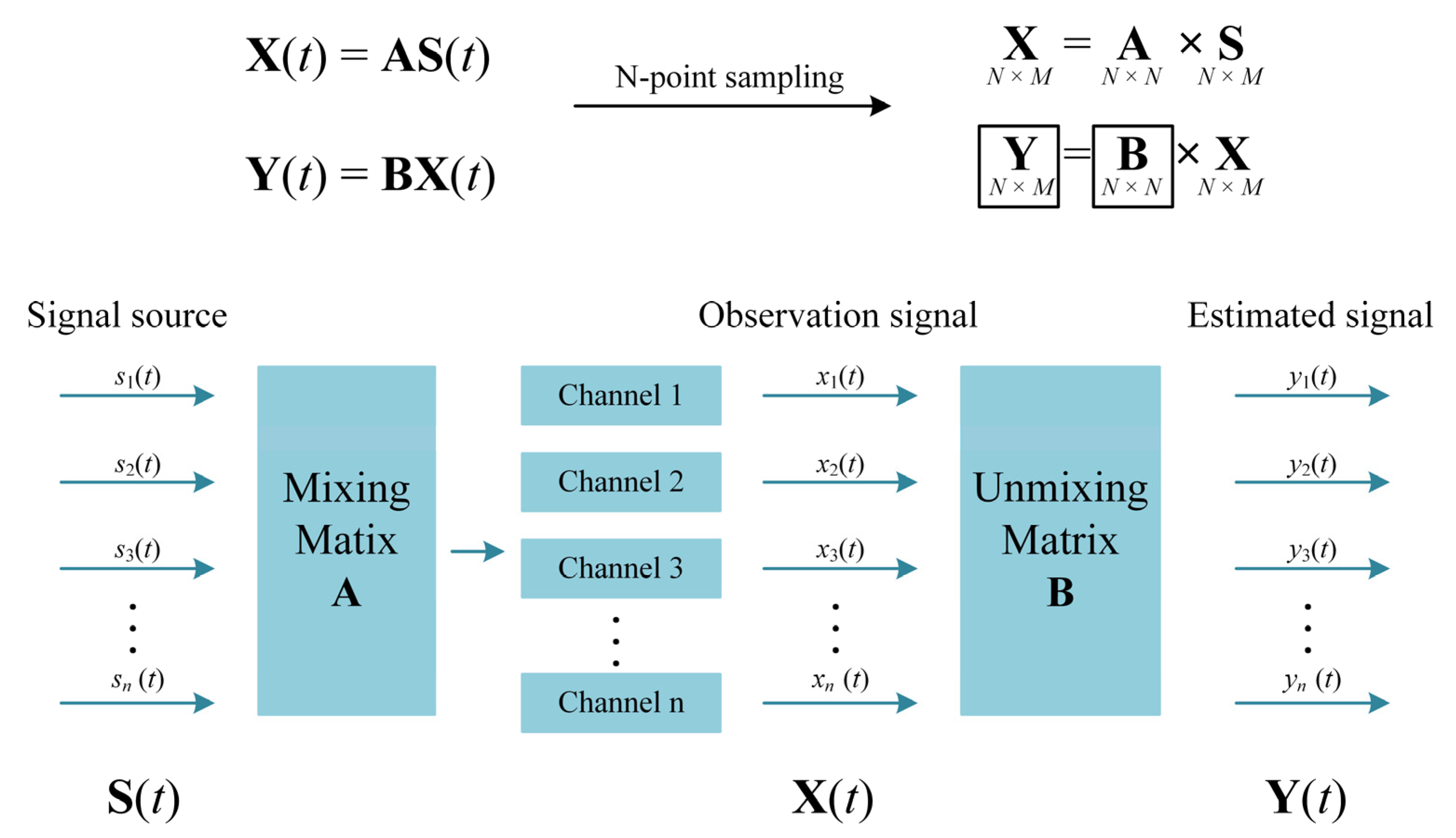
2.3. Independent Component Analysis

ICA is a data-driven approach based on blind source separation (BSS). BSS only assumes that the signal sources are independent non-Gaussian signals, and the relationship between the information of the signal sources and the linear transformation is unknown. ICA is a digital signal processing algorithm developed to solve this problem. Compared to the model-driven approaches, ICA works without prior information about the underlying sources, which allows it to effectively detect some signals that cannot be obtained when using other methods [43,44,45,46].
It is assumed that signal sources are composed of several statistically independent signals that overlap in both temporal and spatial domains, ICA synchronously observes the overlapping signals using multiple channels and decomposes the observed signals into several ICs, after the unmixing, as a set of source signal estimates (Figure 4). The channels exert no influence on the signal, and the number of observed channels is the same as the number of signals. The standard noiseless ICA mathematical model is:
X ( t ) = A S ( t )
where the random vectors X ( t ) = [ X 1 ( t ) , , X M ( t ) ] T represent the observed signals and random vectors S i ( t ) , i = 1 , 2 , , N ; M N represent the source signals, and A is a mixing matrix. The ICA decomposition process can be regarded as the inverse transformation of Equation (9):
Y ( t ) = S ( t ) ^ = B X ( t )
where B is the unmixing matrix. It is assumed that the row vectors in S are statistically independent of each other, their joint probability density function (pdf) is the product of their marginal probability density function, which means that, the joint entropy of each component is the sum of the entropy of each component, such that:
p ( S ) = i = 1 n p ( S i )
where p is the pdf of S, where both A and the source signal S are unknown. However, as long as the output components separated by the unmixing matrix B are statistically independent of each other, this approach is equivalent to separating the source signals.
The basic hypothesis of ICA is that the source signals are statistically independent, allowing for no more than one source with a Gaussian distribution while describing the remaining sources with non-Gaussian distributions. Most of the deformed signals in GNSS coordinate sequences are also non-Gaussian signals, and the non-Gaussian signals are quantized by negentropy. The ICA attempts to create various linear transformations on the observed signals, and the maximum negentropy of the transformed quantity is likely to indicate the source signals [43,46]. Various ICA algorithms have been derived based on this fundamental idea. In this study, we use the FastICA algorithm based on negentropy to estimate the original signals [56,57]. The negentropy is defined as:
J ( X ) = + p G ( X ) ln p G ( X ) d X + + p ( X ) ln p ( X ) d X
where p ( X ) is the pdf of X , and p G ( X ) is the pdf of the Gaussian distribution with the same covariance matrix as p ( X ) . The greater negentropy values are associated with stronger non-Gaussian signals [57,58,59].
A detailed description of the FastICA algorithm procedure is as follows:
  • Centralize and whiten the observed data.
  • Choose an initial weight vector of unit norm w .
  • Update w + through w + = E [ Z g ( w T Z ) ] E [ g ( w T Z ) ] w .
  • Normalize w by w = w + / w + .
  • Return to step 3 if w is not converged.
We can similarly reconstruct the original data set of a GNSS time series of n stations across a period of m days and calculate the CME using the source signals that have been separated by ICA. We can obtain ICs by Y ( t ) = B X ( t ) , assuming that A = B 1 , and X can be obtained by:
X ( t ) = B 1 Y ( t ) = A Y ( t )
The CME based on ICA can thus be given as:
ε ICA = k R R a k y k
where R is a group of temporal components in spatio-temporal filtering.

3. Results

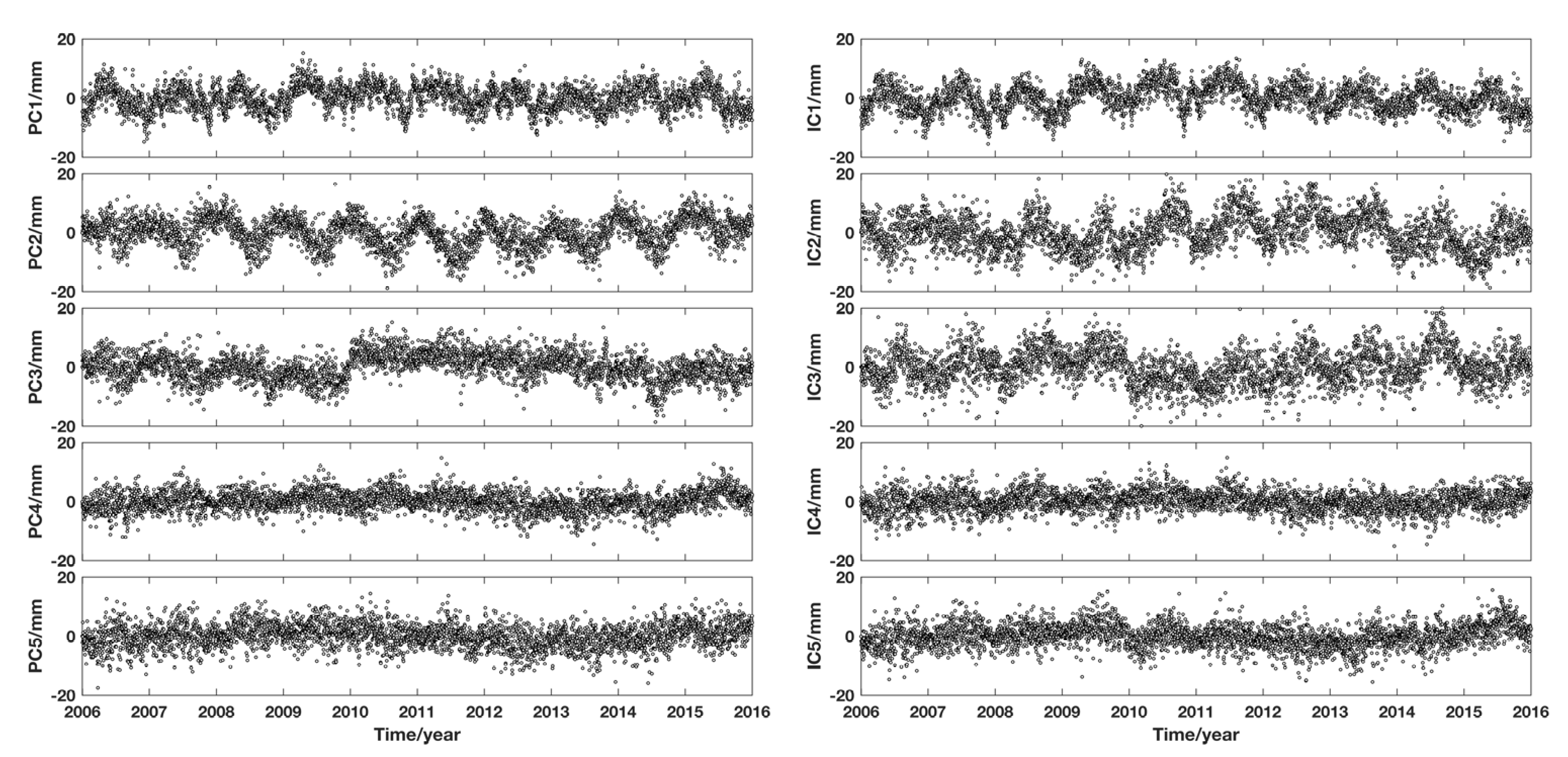
3.1. Common Mode Error Extraction Using PCA/ICA

To intuitively compare the amplitude of each component, the corresponding spatial response is usually divided by the maximum absolute value and scaled to a variation interval of 100 % ~ 100 % , where the scaled amount is multiplied by the corresponding temporal components. An upward movement is a positive response and a downward is a negative response. The results of the first five PCs are shown on the left side of Figure 5, and their corresponding spatial responses are provided in the first row of Figure 6.
We use the standard CME definition provided by Dong et al. [7], in which most stations (50%) for a certain PC mode exhibit a clearly normalized spatial response ( > 25 % ) and the eigenvalue of the mode exceeds 1 % of the collective eigenvalues; it can therefore be considered as a common mode. The spatial response corresponding to the first PC in the first line of Figure 6 displays notably good regional consistency, and its average normalized amplitude (absolute value) is 77.3%. However, the 2nd–5th. PCs do not satisfy this condition. In terms of eigenvalues, Table 1 provides the percentage of the first 10 PC eigenvalues for the total eigenvalues and the cumulative contribution rate (eigenvalues). The first PC accounts for 24.7%, the second PC accounts for 6.5%, and the cumulative contribution rate of the eigenvalues tends to stabilize after the fifth order, which indicates that the first PC is able to represent the most common-mode components. In summary, we define the displacement component caused by the first PC as the CME of the entire GPS network.
We use ICA to process the five components from PCA. The principle is realized using ICA’s fast fixed-point algorithm [57,60]. The first step of the algorithm is to centralize and whiten the observed values before processing. The mixing matrix is orthogonal so as to reduce the number of free parameters. The mixed signals are then linearly transformed to express an unrelated variable with a variance that is equal to 1 (whitening or spheroidizing). This step comprises the pretreatment process of ICA, which is realized by PCA. This is conducted because the number of PCs reserved for the ICA analysis should be lower than the data dimension. The process of trial and error is therefore used to select the appropriate quantity [61]. In this study, the effect of retaining the first five PCs becomes apparent.
The ranking of the ICs obtained by ICA does not correspond to a decrease in the variance. We therefore calculate the average ratio of the GPS_IC displacement in each GPS site calculated by the ICA filtering to the observed time series, in accordance with the procedure described by Liu et al. [19] and Milliner et al. [62]. Smaller ratios are associated with contributions that are more significant, and the ICs are reordered in ascending order. The corresponding spatial response of each IC is normalized according to the absolute value of its maximum value so that the comparison is more accurate. The IC time series and the corresponding spatial response value, after the IC, is multiplied by the normalization factor, shown on the right in Figure 5 and in the second row of Figure 6. The first two ICs are evidently the largest of the original data according to the previous definition of the CME, and their spatial response values display the same sign. We can therefore locate the displacement caused by these two components as the CME of the entire GPS network in ICA filtering.
After calculating the CME, we subtract its influence on each station from the original time series. The filtering effect can be described by the reduction rate of the root mean square (RMS) of the residual time series (Figure 7). The results in Table 2 reveal that after PCA and ICA filtering, the average RMS values are reduced by approximately 14% and 17%, respectively. These two methods can therefore be used to effectively improve the signal-to-noise ratio of the residual time series.
Figure 7 shows the decline of the RMS value of the residual time series at each station after ICA filtering. Figure 7 also presents notable differences in the ICA filtering effect between the east and west. The RMS reduction rate in the west is relatively large, whereas that in the east is small, which is partially due to topography. There are many mountains on the eastern side of Taiwan and the stations are sparsely distributed, whereas the western side is relatively flat and the stations are relatively dense. Another explanation is the orogenic processes, as there is topographic uplift in the eastern region [63] and sinking in the southwest region due to groundwater extraction [64]. This phenomenon can also be observed in the second-order PCs obtained via PCA filtering, and the station response indicates notable local variation characteristics, as shown in PC2 in the first line of Figure 6.

3.2. Noise Analysis of GNSS Coordinate Time Series

In the noise analysis of the Taiwan GNSS time series, for the original time series of each station, we fit the offsets in advance, interpolate the original data, and then analyze the power spectrum of the noise series. The results are presented in Figure 8. Due to the large volume of data, this study uses the GS39 station as an example to elaborate on an explanation. It can be seen that the power spectrum at low and high frequencies of the noise series presents different peaks and demonstrates a clear linear trend term. The spectral energy in the low-frequency band is higher than that in high-frequency band. The spectral exponent of this component is −0.67, which indicates that the noise of this station is influenced by colored noise. Through piecewise fitting, the slope of this component is approximately approached, yielding −1 at a low frequency and 0 at a higher frequency. The low-frequency result possesses the characteristics of flicker noise, and the high-frequency result possesses the characteristics of white noise. It can thus be estimated that the noise type of this point is a combination type of white noise and flicker noise.

4. Discussion

4.1. Potential Geophysical Interpretation of the CME

We note that although the RMS reduction results are similar, the PCA and ICA filtering processes exhibit different spatial and temporal patterns. Previous studies have also revealed that PCA-derived CMEs are not completely unrelated to local effects or random noise. The decomposition of similar contribution components in an actual network residual time series is difficult to achieve using PCA, and we cannot identify potential geophysical mechanisms or study the subtle signals in GPS observations [29]. In contrast, there is a high correlation between the common mode components extracted by ICA and the simulated surface mass loading deformation. An important criterion to better understand and describe the differences between the ICA and PCA results is the extent to which the temporal and spatial patterns of annual crustal deformation, caused by mass loadings of various geophysical sources, are restored by using these two methods.
We submitted requests for real-time solutions for the ATML, and LWS 3-D displacement files from 44 stations in Taiwan between 1 January 2006 and 31 December 2015 using the online solution function of the IMLS (http://massloading.net/, accessed on 2 August 2021) [65,66,67,68]. For ATML and LWS, we used the GEOS-FPIT model developed by the Global Modeling and Assimilation Office at NASA Goddard Space Flight Center, which considers a time range from 1 January 2000 to present, that is updated several times per day. The model resolution is 0.50° × 0.625° × 72 layers × 3 h. We obtained the displacement time series in the center-of-figure frame.
We averaged all of the loading series displacements into the daily results, and we calculated the average GPS_IC1 and GPS_IC2,comparing it with the average ATML and LWS. As indicated in Figure 9, GPS_IC is the outer product of the IC and its corresponding spatial response. We note that ATML and LWS are consistent in terms of their amplitude and phase with GPS_IC1 and GPS_IC2, respectively. The correlation coefficients of these two temporal patterns are 0.58 and 0.4, respectively. We therefore suggest that atmospheric and hydrological mass loading are the main components of the CME in the Taiwan GPS network, which can be reflected by the IC extracted by ICA spatio-temporal filtering. Although IC1 and IC2 can be interpreted by ATML and LWS, other temporal components are statistically independent, and their unretrieved information still requires further study.

4.2. Effect of Removing the CME

We then use the Hector software [69] to analyze the 44 noise sequences with only the offsets corrected using the white-plus-power law (W + PL) model. We do not fix the spectral index, but treat it as an unknown factor, and solve it alongside the linear, annual, and semi-annual periodic terms [14]. On this basis, we subtract the CME after ICA filtering and analyze the obtained noise sequence, as shown in Table 3. We also analyze the power spectrum of the original noise sequence, PCA filtered noise sequence, and ICA filtered noise sequence of station GS39, as shown in Figure 10. The ICA filtering approach is observed is more useful than the PCA in terms of the amplitude of the annual term.
Table 3 lists the estimated parameters and noise terms of the 44 stations in Taiwan. We can see that the PL amplitude is reduced by an average of approximately 27.8% after ICA filtering, which indicates that the filtering has a certain suppression effect on noise. However, there is not an obvious change in the amplitude of the white noise (W), which indicates that it originated locally. The amplitude of annual and semi-annual periodic terms decreased by approximately 60% and 18%, respectively. Before and after the filtering, the average spectral index shifted from −0.77 to −0.92, which is consistent with the result of Rao et al. [70], indicating that the noise model of the Taiwan GPS data is closer to the white-plus-flicker noise (W+FN) model with a spectral index of −1.

5. Conclusions

We use PCA and ICA approaches to analyze the vertical coordinate time series of 44 sites in Taiwan island in China from 2006 to 2016. The results are summarized as follows.
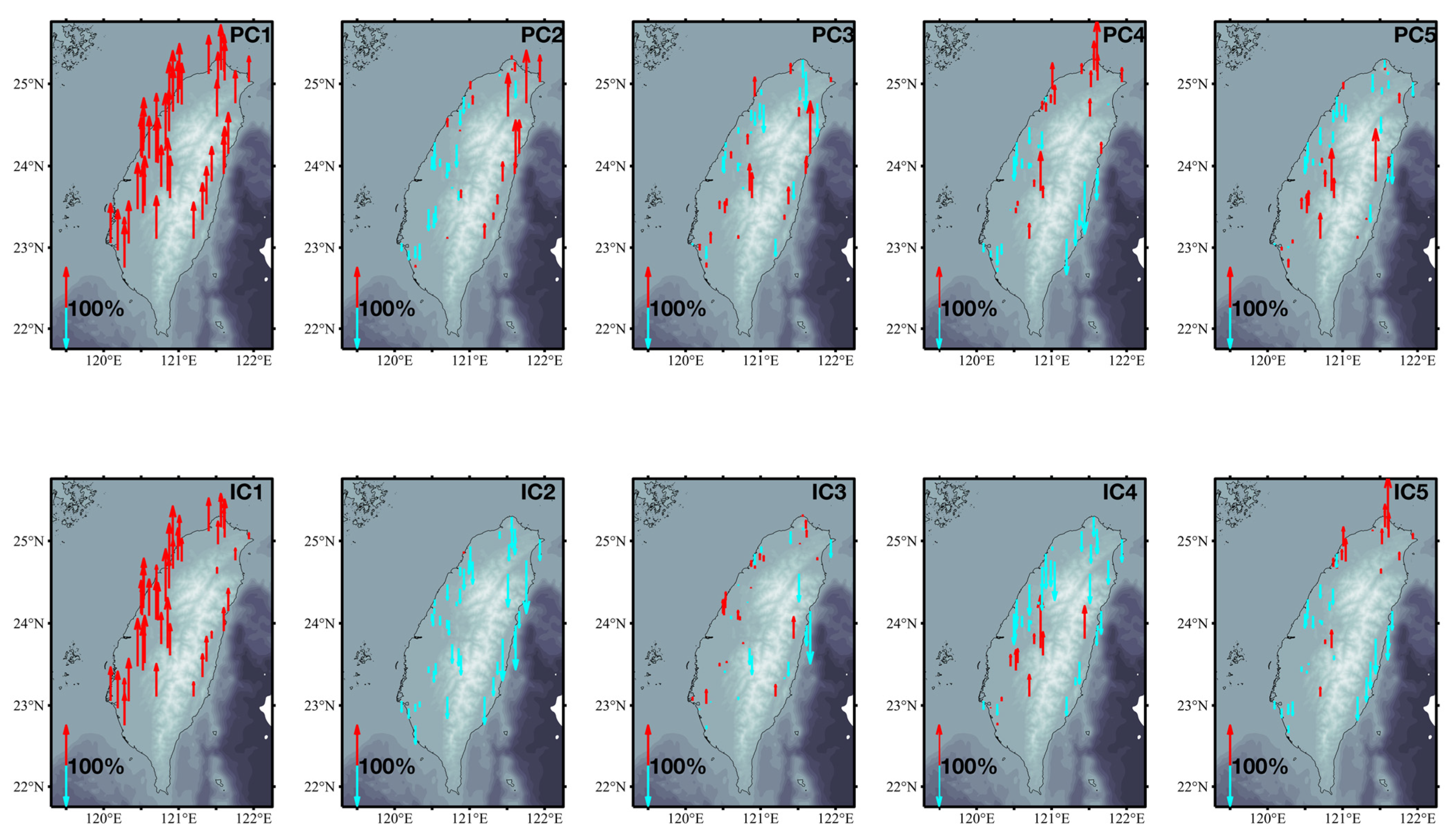
  • Both PCA and ICA can effectively remove the CME. The average RMS of PCA and ICA in the U direction shifted from 6.47 mm to 5.58 mm and 5.40 mm, respectively, a decreased by approximately 14% and 17%. However, the CMEs of the two approaches reveal notable differences in their temporal and spatial characteristics. Figure 6 shows that the PCA separates only one CME and the ICA separates two CMEs. We therefore believe that PCA may eliminate the original site information, whereas ICA retains more original site information.
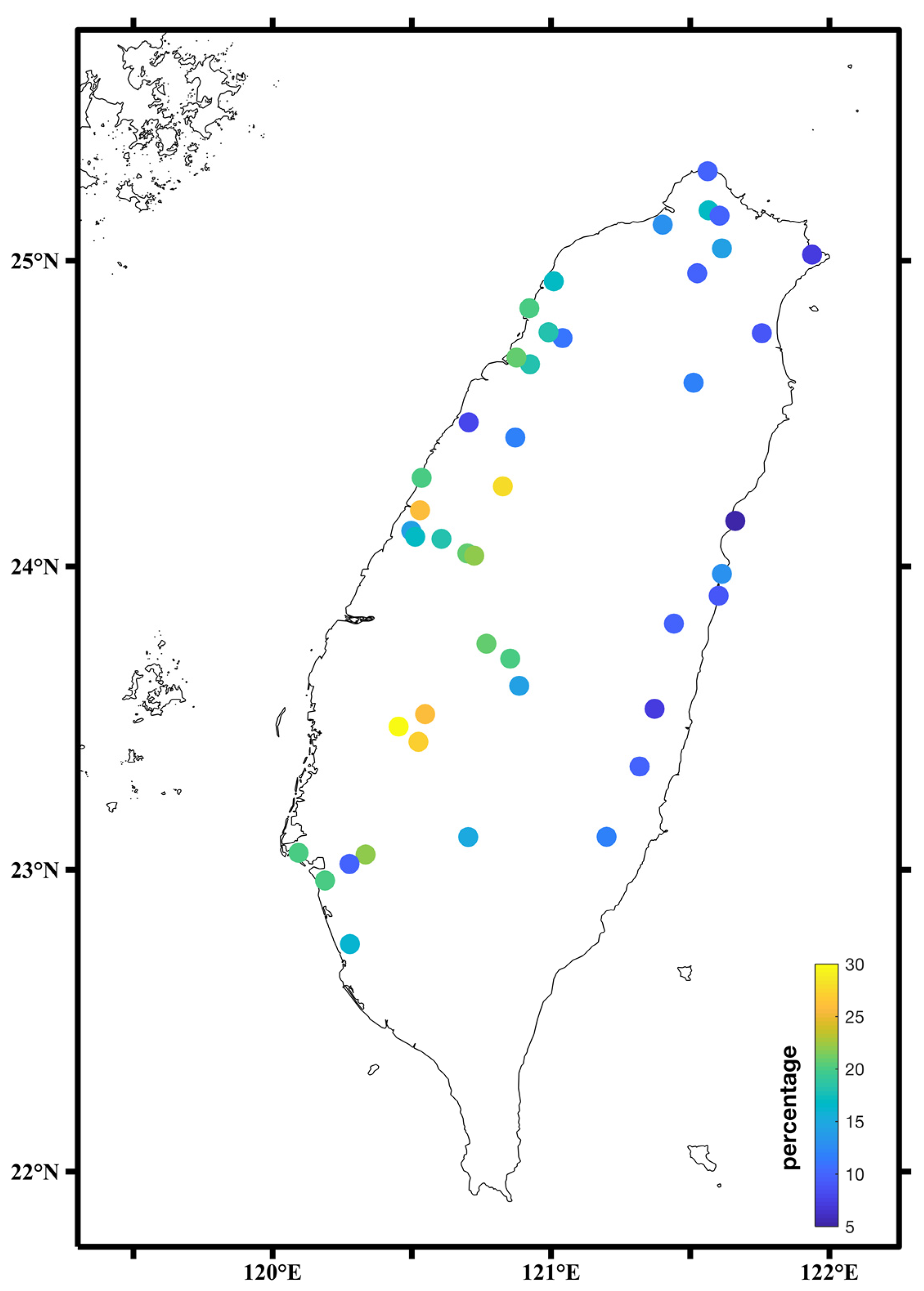
  • There are notable differences in the ICA filtering effect between the east and west of Taiwan. The RMS reduction rate in the west is relatively large, whereas that in the east small, which is partially due to topography. There are many mountains on the eastern side of Taiwan and the stations are sparsely distributed, whereas the western side is relatively flat and the stations are relatively dense. Another explanation is the orogenic processes, as there is a topographic uplift in the eastern region and sinking in the southwest region due to groundwater extraction.
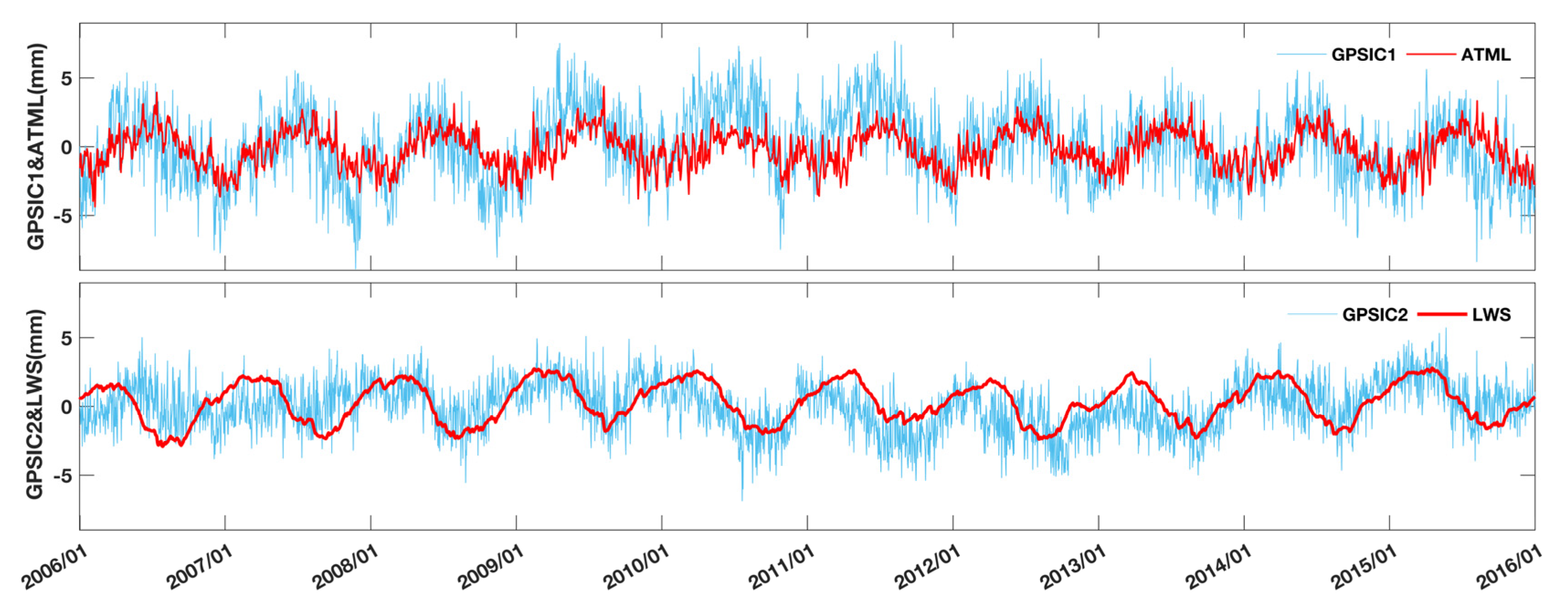
  • To explore the possible geophysical sources of ICA’s CMEs, we compare the CMEs of ICA with the predicted average loading displacements caused by changes in the atmospheric and hydrological loadings. It is found that GPS_IC1 and ATML, and GPS_IC2 and LWS are consistent in terms of amplitude and characteristics. The correlation between GPS_IC1 and ATML is 0.55, and the correlation coefficient between GPS_IC2 and LWS is 0.40. This indicates that seasonal changes in Taiwan are related to the movement of water in addition to atmospheric pressure.
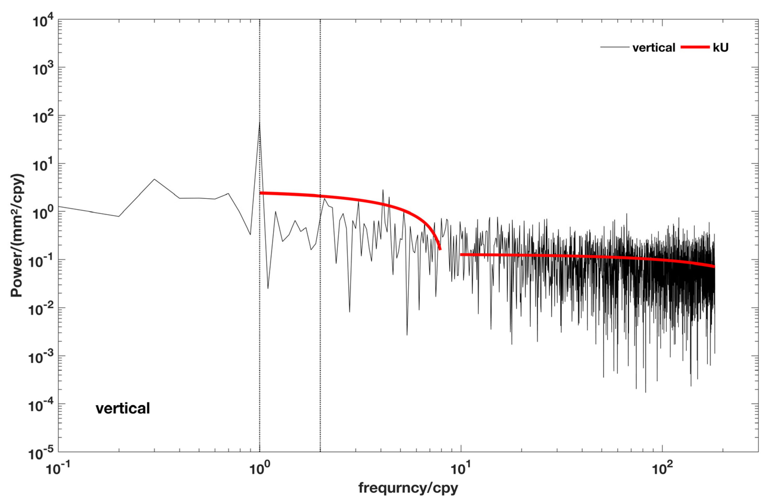
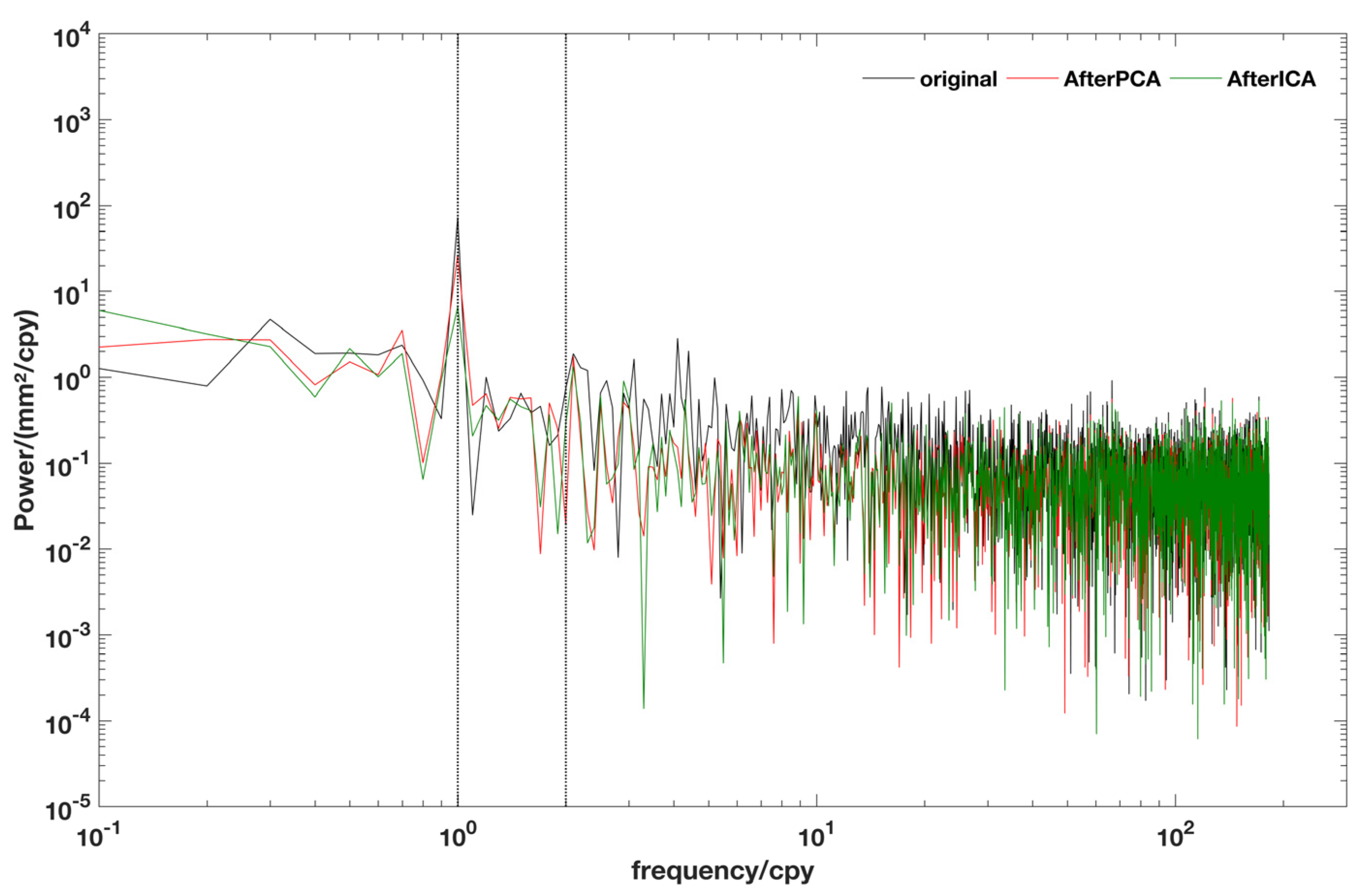
  • We used Hector software to analyze the noise characteristics of the time series of all stations prior to filtering. The average spectral index shifted from -0.72 to -0.92, which indicates that the most suitable noise model in Taiwan is W + FN. Filtering can also effectively reduce PL noise. After filtering, PL noise is reduced by an average of approximately 28%. The average annual cycle item is also significantly reduced by approximately 60%. ICA filtration is more advantageous than PCA filtration. The noise sequence filtered by ICA and PCA at the GS39 station was analyzed to verify the above conclusions.

Author Contributions

All authors contributed significantly to the manuscript. Conceptualization, X.M., B.L. and W.D.; methodology, X.M. and B.L.; validation, X.M. and B.L.; formal analysis, X.M.; investigation, X.M.; resources, B.L. and W.D.; data curation, X.X.; writing—original draft preparation, X.M.; writing—review and editing, B.L., W.D., C.K. and X.X.; supervision, W.D., C.K. and X.X.; funding acquisition, B.L. All authors have read and agreed to the published version of the manuscript.

Funding

This work is funded by the National Natural Science Foundation of China (Grant No. 41904003, 41774040, 41674011), the Natural Science Foundation of Hunan Province, China (Grant No. 2020JJ5571) and Open Fund of Engineering Laboratory of Spatial Information Technology of Highway Geological Disaster Early Warning in Hunan Province (Changsha University of Science & Technology) (Grant No. KFJ190602).

Data Availability Statement

The GPS data used in this work can be obtained from the GPS Lab web application (http://gps.earth.sinica.edu.tw, accessed on 2 August 2021) of the Institute of Earth Sciences, Academia Sinica, Taiwan. This application requires a simple registration process to access the data. You can download the three-component continuous GPS time series data of all the sites through the “download time series” button. The pre-calculated ATML and LWS displacement data sets were obtained from the International Mass Loading Service Web application (http://massloading.net/, accessed on 2 August 2021) Explore individual loadings, used in the “GEOS-FPIT” model, the “Center of figure” frame, and the time range is in “Between 2006.01.01_00:00” and “2016.01.01_00:00”. Site file uses our solved XYZ coordinate file. The displacement is provided every 3 h and is stored in a total of 120 .eph files at all 44 sites. The file name contains the corresponding timestamp. We extract the U-component displacement from each file to form the original time series data set for our spatio-temporal analysis. The time series of the GPS stations used in this paper are uploaded to Figshare, and readers can download the data from: https://figshare.com/articles/dataset/data_for_EES_rar/13490442, accessed on 2 August 2021.

Conflicts of Interest

The authors declare no conflict of interest.

References

  1. Bock, Y.; Melgar, D. Physical applications of GPS geodesy: A review. Rep. Prog. Phys. 2016, 79, 106801. [Google Scholar] [CrossRef]
  2. He, X.; Montillet, J.P.; Fernandes, R.; Bos, M.; Yu, K.; Hua, X.; Jiang, W. Review of current GPS methodologies for producing accurate time series and their error sources. J. Geodyn. 2017, 106, 12–29. [Google Scholar] [CrossRef]
  3. Li, Z.; Jiang, W.; Liu, H. Noise Model Establishment and Analysis of IGS Reference Station Coordinate Time Series inside China. Acta Geod. Cartogr. Sin. 2012, 41, 496–503. [Google Scholar]
  4. Huang, L. Noise properties in time series of coordinate component at gps fiducial stations. J. Geod. Geodyn. 2006, 26, 31–34. [Google Scholar]
  5. Mao, A.; Harrison, C.G.A.; Dixon, T.H. Noise in GPS coordinate time series. J. Geophys. Res. 1999, 104, 2797–2816. [Google Scholar] [CrossRef] [Green Version]
  6. Wdowinski, S.; Bock, Y.; Zhang, J.; Fang, P.; Genrich, J. Southern California permanent GPS geodetic array: Spatial filtering of daily positions for estimating coseismic and postseismic displacements induced by the 1992 Landers earthquake. J. Geophys. Res. Solid Earth 1997, 102, 18057–18070. [Google Scholar] [CrossRef]
  7. Dong, D.; Fang, P.; Bock, Y.; Webb, F.; Prawirodirdjo, L.; Kedar, S.; Jamason, P. Spatiotemporal filtering using principal component analysis and Karhunen-Loeve expansion approaches for regional GPS network analysis. J. Geophys. Res. Solid Earth 2006, 111, B03405. [Google Scholar] [CrossRef] [Green Version]
  8. Gruszczynski, M.; Klos, A.; Bogusz, J. A Filtering of Incomplete GNSS Position Time Series with Probabilistic Principal Component Analysis. Pure. Appl. Geophys. 2018, 175, 1841–1867. [Google Scholar] [CrossRef]
  9. King, M.A.; Altamimi, Z.; Boehm, J.; Bos, M.; Dach, R.; Elosegui, P.; Fund, F.; Hernández-Pajares, M.; Lavallee, D.; Cerveira, P.J.M. Improved constraints on models of glacial isostatic adjustment: A review of the contribution of ground-based geodetic observations. Surv. Geophys. 2010, 31, 465–507. [Google Scholar] [CrossRef]
  10. Zhu, Z.; Zhou, X.; Deng, L.; Wang, K.; Zhou, B. Quantitative analysis of geophysical sources of common mode component in CMONOC GPS coordinate time series. Adv. Space Res. 2017, 60, 2896–2909. [Google Scholar] [CrossRef]
  11. Bogusz, J.; Gruszczynski, M.; Figurski, M.; Klos, A. Spatio-temporal filtering for determination of common mode error in regional GNSS networks. Open Geosci. 2015, 7, 140–148. [Google Scholar] [CrossRef] [Green Version]
  12. Nikolaidis, R. Observation of Geodetic and Seismic Deformation with the Global Positioning System. Ph.D. Thesis, University of California, San Diego, CA, USA, 2002. [Google Scholar]
  13. Márquez-Azúa, B.; DeMets, C. Crustal velocity field of Mexico from continuous GPS measurements, 1993 to June 2001: Implications for the neotectonics of Mexico. J. Geophys. Res. Solid Earth 2003, 108, 2450. [Google Scholar] [CrossRef]
  14. Williams, S.D.P.; Bock, Y.; Fang, P.; Jamason, P.; Nikolaidis, R.M.; Prawirodirdjo, L.; Miller, M.; Johnson, D.J. Error analysis of continuous GPS position time series. J. Geophys. Res. Solid Earth 2004, 109, B03412. [Google Scholar] [CrossRef] [Green Version]
  15. Tian, Y.; Shen, Z.-K. Extracting the regional common-mode component of GPS station position time series from dense continuous network. J. Geophys. Res. Solid Earth 2016, 121, 1080–1096. [Google Scholar] [CrossRef]
  16. Serpelloni, E.; Faccenna, C.; Spada, G.; Dong, D.; Williams, S.D.P. Vertical GPS ground motion rates in the Euro-Mediterranean region: New evidence of velocity gradients at different spatial scales along the Nubia-Eurasia plate boundary. J. Geophys. Res. Solid Earth 2013, 118, 6003–6024. [Google Scholar] [CrossRef] [Green Version]
  17. He, X.; Hua, X.; Yu, K.; Xuan, W.; Lu, T.; Zhang, W.; Chen, X. Accuracy enhancement of GPS time series using principal component analysis and block spatial filtering. Adv. Space Res. 2015, 55, 1316–1327. [Google Scholar] [CrossRef]
  18. Liu, B.; Dai, W.; Peng, W.; Meng, X. Spatiotemporal analysis of GPS time series in vertical direction using independent component analysis. Earth Planets Space 2015, 67, 189. [Google Scholar] [CrossRef] [Green Version]
  19. Liu, B.; Dai, W.; Liu, N. Extracting seasonal deformations of the Nepal Himalaya region from vertical GPS position time series using Independent Component Analysis. Adv. Space Res. 2017, 60, 2910–2917. [Google Scholar] [CrossRef]
  20. Li, W.; Shen, Y. The Consideration of Formal Errors in Spatiotemporal Filtering Using Principal Component Analysis for Regional GNSS Position Time Series. Remote Sens. 2018, 10, 534. [Google Scholar] [CrossRef] [Green Version]
  21. Tan, W.; Chen, J.; Dong, D.; Qu, W.; Xu, X. Analysis of the Potential Contributors to Common Mode Error in Chuandian Region of China. Remote. Sens. 2020, 12, 751. [Google Scholar] [CrossRef] [Green Version]
  22. Yuan, L.G.; Dong, X.; Chen, W.; Guo, Z.; Chen, S.; Hong, B.; Zhou, J. Characteristics of daily position time series from the Hong Kong GPS fiducial network. Chin. J. Geophys. 2008, 51, 1372–1384. [Google Scholar] [CrossRef]
  23. Shen, Y.; Li, W.; Xu, G.; Li, B. Spatiotemporal filtering of regional GNSS network’s position time series with missing data using principle component analysis. J. Geod. 2014, 88, 1–12. [Google Scholar] [CrossRef]
  24. Li, W.; Shen, Y.; Li, B. Weighted spatiotemporal filtering using principal component analysis for analyzing regional GNSS position time series. Acta Geod. Geophys. 2015, 50, 419–436. [Google Scholar] [CrossRef] [Green Version]
  25. Kreemer, C.; Blewitt, G. Robust estimation of spatially varying common-mode components in GPS time-series. J. Geod. 2021, 95, 1–19. [Google Scholar] [CrossRef]
  26. Liu, B.; King, M.; Dai, W. Common mode error in Antarctic GPS coordinate time-series on its effect on bedrock-uplift estimates. Geophys. J. Int. 2018, 214, 1652–1664. [Google Scholar] [CrossRef]
  27. Zhou, M.; Guo, J.; Liu, X.; Shen, Y.; Zhao, C. Crustal movement derived by GNSS technique considering common mode error with MSSA. Adv. Space Res. 2020, 66, 1819–1828. [Google Scholar] [CrossRef]
  28. Pan, Y.; Chen, R.; Ding, H.; Xu, X.; Zheng, G.; Shen, W.; Xiao, Y.; Li, S. Common Mode Component and Its Potential Effect on GPS-Inferred Three-Dimensional Crustal Deformations in the Eastern Tibetan Plateau. Remote. Sens. 2019, 11, 1975. [Google Scholar] [CrossRef] [Green Version]
  29. Yan, J.; Dong, D.; Burgmann, R.; Materna, K.; Tan, W.; Peng, Y.; Chen, J. Separation of Sources of Seasonal Uplift in China Using Independent Component Analysis of GNSS Time Series. J. Geophys. Res. Solid Earth 2019, 124, 11951–11971. [Google Scholar] [CrossRef]
  30. Gualandi, A.; Serpelloni, E.; Belardinelli, M.E. Blind source separation problem in GPS time series. J. Geod. 2016, 90, 323–341. [Google Scholar] [CrossRef]
  31. Gualandi, A.; Avouac, J.P.; Galetzka, J.; Genrich, J.F.; Blewitt, G.; Adhikari, L.B.; Koirala, B.P.; Gupta, R.; Upreti, B.N.; Pratt-Sitaula, B.J.T. Pre-and post-seismic deformation related to the 2015, Mw7. 8 Gorkha earthquake, Nepal. Tectonophysics 2017, 714, 90–106. [Google Scholar] [CrossRef]
  32. Bian, Y.; Yue, J.; Ferreira, V.G.; Cong, K.; Cai, D. Common Mode Component and Its Potential Effect on GPS-Inferred Crustal Deformations in Greenland. Pure. Appl. Geophys. 2021, 178, 1805–1823. [Google Scholar] [CrossRef]
  33. Deng, L.; Chen, H.; Ren, J.; Liao, Y. Long-term and seasonal displacements inferred from the regional GPS coordinate time series: Case study in Central China Hefei City. Earth Sci. Inform. 2020, 13, 71–81. [Google Scholar] [CrossRef]
  34. An, J.; Zhang, B.; Ai, S.; Wang, Z.; Feng, Y. Evaluation of vertical crustal movements and sea level changes around Greenland from GPS and tide gauge observations. Acta Oceanol. Sin. 2021, 40, 4–12. [Google Scholar] [CrossRef]
  35. Zhang, T.; Shen, W.; Pan, Y.; Luan, W. Study of seasonal and long-term vertical deformation in Nepal based on GPS and GRACE observations. Adv. Space Res. 2018, 61, 1005–1016. [Google Scholar] [CrossRef]
  36. Ma, C.; Li, F.; Zhang, S.; Lei, J.; Dong-Chen, E.; Hao, W.; Zhang, Q. The coordinate time series analysis of continuous GPS stations in the Antarctic Peninsula with consideration of common mode error. Chin. J. Geophys. 2016, 59, 2783–2795. [Google Scholar]
  37. Zhang, K.; Wang, Y.; Gan, W.; Liang, S. Impacts of Local Effects and Surface Loads on the Common Mode Error Filtering in Continuous GPS Measurements in the Northwest of Yunnan Province, China. Sensors 2020, 20, 5408. [Google Scholar] [CrossRef]
  38. Ming, F.; Yang, Y.; Zeng, A.; Zhao, B. Spatiotemporal filtering for regional GPS network in China using independent component analysis. J. Geod. 2017, 91, 419–440. [Google Scholar] [CrossRef]
  39. Kumar, U.; Chao, B.F.; Chang, E.T.Y. What Causes the Common-Mode Error in Array GPS Displacement Fields: Case Study for Taiwan in Relation to Atmospheric Mass Loading. Earth Space Sci. 2020, 7, e2020EA001159. [Google Scholar] [CrossRef]
  40. Yu, S.; Chen, H.; Kuo, L. Velocity field of GPS stations in the Taiwan area. Tectonophysics 1997, 274, 41–59. [Google Scholar] [CrossRef]
  41. Yu, S.; Hsu, Y.; Kuo, L.; Chen, H.; Liu, C. GPS measurement of postseismic deformation following the 1999 Chi-Chi, Taiwan, earthquake. J. Geophys. Res. 2003, 108, 2520–2539. [Google Scholar] [CrossRef] [Green Version]
  42. Yi-Ben, T. Seismotectonics of Taiwan. Tectonophysics 1986, 125, 17–37. [Google Scholar] [CrossRef]
  43. Comon, P. Independent component analysis, a new concept? Signal. Process. 1994, 36, 287–314. [Google Scholar] [CrossRef]
  44. Comon, P.; Jutten, C.; Herault, J. Blind separation of sources, Part II: Problems statement. Signal. Process. 1991, 24, 11–20. [Google Scholar] [CrossRef]
  45. Herault, J.; Jutten, C. Space or time adaptive signal processing by neural network models. Am. Inst. Phys. 1986, 151, 206–211. [Google Scholar]
  46. Jutten, C.; Herault, J. Blind separation of sources, part I: An adaptive algorithm based on neuromimetic architecture. Signal. Process. 1991, 24, 1–10. [Google Scholar] [CrossRef]
  47. Gazeaux, J.; Williams, S.; King, M.; Bos, M.; Dach, R.; Deo, M.; Moore, A.; Ostini, L.; Petrie, E.; Roggero, M.; et al. Detecting offsets in GPS time series: First results from the detection of offsets in GPS experiment. J. Geophys. Res. Solid Earth 2013, 118, 2397–2407. [Google Scholar] [CrossRef] [Green Version]
  48. Wang, W.; Qiao, X.; Wang, D.; Chen, Z.; Yu, P.; Lin, M.; Chen, W. Spatiotemporal noise in GPS position time-series from Crustal Movement Observation Network of China. Geophys. J. Int. 2019, 216, 1560–1577. [Google Scholar] [CrossRef]
  49. Wang, F.; Zhang, P.; Sun, Z.; Zhang, Q.; Liu, J. Analysis the Influence of Modulated Amplitude on Common Mode Error Based on GPS Data. ISPRS-Int. Arch. Photogramm. Remote. Sesing Spat. Inf. Sci. 2021, 43, 153–158. [Google Scholar] [CrossRef]
  50. Zhu, Z.; Zhou, X.; Liu, J. Noise analysis of common mode error in CMONOC GPS coordinate time series. In Proceedings of the 2017 Forum on Cooperative Positioning and Service (CPGPS), Harbin, China, 19–21 May 2017; IEEE: Piscataway, NJ, USA, 2017; pp. 190–193. [Google Scholar]
  51. Klos, A.; Olivares, G.; Teferle, F.N.; Hunegnaw, A.; Bogusz, J. On the combined effect of periodic signals and colored noise on velocity uncertainties. Gps Solut. 2017, 22, 1–13. [Google Scholar] [CrossRef] [Green Version]
  52. Jiang, W.; Ma, J.; Li, Z.; Zhou, X.; Zhou, B. Effect of removing the common mode errors on linear regression analysis of noise amplitudes in position time series of a regional GPS network & a case study of GPS stations in Southern California. Adv. Space Res. 2018, 61, 2521–2530. [Google Scholar]
  53. He, X.; Bos, M.S.; Montillet, J.P.; Fernandes, R.M.S. Investigation of the noise properties at low frequencies in long GNSS time series. J. Geod. 2019, 93, 1271–1282. [Google Scholar] [CrossRef]
  54. Santamaría-Gómez, A.; Ray, J. Chameleonic Noise in GPS Position Time Series. J. Geophys. Res. Solid Earth 2021, 126, e2020JB019541. [Google Scholar] [CrossRef]
  55. Dong, D.; Chen, J.; Wang, J. The GNSS High. Precision Positioning Principle; Science Press: Beijing, China, 2018; pp. 253–260. [Google Scholar]
  56. Hyvärinen, A. Fast and robust fixed-point algorithms for independent component analysis. IEEE Trans. Neural Netw. 1999, 10, 626–634. [Google Scholar] [CrossRef] [PubMed] [Green Version]
  57. Hyvärinen, A.; Oja, E. A fast fixed-point algorithm for independent component analysis. Neural Comput. 1997, 9, 1483–1492. [Google Scholar] [CrossRef]
  58. Bell, A.; Sejnowski, T. An information-maximization approach to blind separation and blind deconvolution. Neural Comput. 1995, 7, 1129–1159. [Google Scholar] [CrossRef]
  59. Yang, F.; Hong, B. Theory and Application of Independent Component Analysis; Tsinghua University Press: Beijing, China, 2006. [Google Scholar]
  60. Hyvärinen, A.; Oja, E. Independent component analysis: Algorithms and applications. Neural Comput. 2000, 13, 411–430. [Google Scholar] [CrossRef] [Green Version]
  61. Barnie, T.; Oppenheimer, C. Extracting high temperature event radiance from satellite images and correcting for saturation using independent component analysis. Remote. Sens. Env. 2015, 158, 56–68. [Google Scholar] [CrossRef] [Green Version]
  62. Milliner, C.; Materna, K.; Burgmann, R.; Fu, Y.; Moore, A.; Bekaert, D.; Adhikari, S.; Argus, D. Tracking the weight of Hurricane Harvey’s stormwater using GPS data. Sci. Adv. 2018, 4, eaau2477. [Google Scholar] [CrossRef] [Green Version]
  63. Hsu, Y.; Lai, Y.; You, R.; Chen, H.; Teng, L.; Tsai, Y.; Tang, C.; Su, H. Detecting rock uplift across southern Taiwan mountain belt by integrated GPS and leveling data. Tectonophysics 2018, 744, 275–284. [Google Scholar] [CrossRef]
  64. Hu, J.; Chu, H.; Hou, C.; Lai, T.; Chen, R.; Nien, P. The contribution to tectonic subsidence by groundwater abstraction in the Pingtung area, southwestern Taiwan as determined by GPS measurements. Quat. Int. 2006, 147, 62–69. [Google Scholar] [CrossRef]
  65. Dobslaw, H.; Bergmann-Wolf, I.; Dill, R.; Poropat, L.; Thomas, M.; Dahle, C.; Esselborn, S.; Koenig, R.; Flechtner, F. A new high-resolution model of non-tidal atmosphere and ocean mass variability for de-aliasing of satellite gravity observations: AOD1B RL06. Geophys. J. Int. 2017, 211, 263–269. [Google Scholar] [CrossRef] [Green Version]
  66. Petrov, L. The International Mass Loading Service. In REFAG 2014; Springer: Cham, Switzerland, 2015; pp. 79–83. [Google Scholar]
  67. Petrov, L.; Boy, J. Study of the atmospheric pressure loading signal in very long baseline interferometry observations. J. Geophys. Res. 2004, 109, 409. [Google Scholar] [CrossRef] [Green Version]
  68. Rienecker, M.; Suarez, M.; Todling, R.; Bacmeister, J.; Takacs, L.; Liu, H.; Gu, W.; Sienkiewicz, M.; Koster, R.; Gelaro, R. The GEOS-5 Data Assimilation System: Documentation of Versions 5.0. 1, 5.1. 0, and 5.2. 0; Technical Report Series on Global Modeling and Data Assimilation Volume 27; NASA: Washington, DC, USA, December 2008.
  69. Bos, M.; Fernandes, R.; Williams, S.; Bastos, L. Fast error analysis of continuous GNSS observations with missing data. J. Geod. 2013, 87, 351–360. [Google Scholar] [CrossRef] [Green Version]
  70. Rao, R. Noise in GPS coordinate time series II. Compilation by the Central Weather Bureau of the Ministry of Communications. 2014; Volume 64, pp. 281–327. Available online: https://scweb.cwb.gov.tw/Uploads/Reports/MOTC-CWB-103-E-04.pdf (accessed on 2 August 2021). (In Chinese)
Figure 1. Taiwan continuous global positioning system (CGPS) network. The black, green, blue, and purple circles represent CGPS sites operated by the Central Weather Bureau (CWB), the Institute of Earth Sciences (IES), the Central Geological Survey (CGS) and the Water Resources Agency (WRA) and other research units. Among them, the sites represented by red triangles are used in this ICA/PCA study.
Remotesensing 13 04221 g001
Figure 2. Data availability of the 44 GPS sites. Blanks represent the missing data.
Remotesensing 13 04221 g002
Figure 3. Original GPS time series (left) and preprocessing sequence of the CHKU, JUNA, S101, SFON, and SHAN stations (right).
Remotesensing 13 04221 g003
Figure 4. Schematic illustration of independent component analysis.
Remotesensing 13 04221 g004
Figure 5. Five components extracted from Taiwan PCA (left) and ICA (right).
Remotesensing 13 04221 g005
Figure 6. Spatial response of five PCs (first row) and ICs (second row) at each site in Taiwan. The red arrow represents the positive spatial response, and the blue arrow represents the negative spatial response.
Remotesensing 13 04221 g006
Figure 7. RMS reduction percentage of residual time series after ICA filtering.
Remotesensing 13 04221 g007
Figure 8. U component power spectrum of the GS39 site noise sequence. The black line represents the power spectrum, and the red line represents the slope.
Remotesensing 13 04221 g008
Figure 9. Comparison of the GPS_ICs (calculated with IC1 and IC2) and mass loading deformation signals (ATML and LWS). The upper figure shows GPS_IC1 and the ATML, and the lower figure shows GPS_IC2 and the LWS.
Remotesensing 13 04221 g009
Figure 10. Comparison of the power spectrum of the GS39 site noise sequence and noise sequence filtered by PCA and ICA.
Remotesensing 13 04221 g010
Table 1. Individual contribution rate and cumulative contribution rate of the top ten PCs.
Order of PCsIndividual
Contribution Rate (%)
Cumulative
Contribution Rate (%)
124.724.7
26.531.2
34.635.8
43.739.5
53.643.1
63.046.1
72.748.8
82.551.3
92.453.7
102.356.0
Table 2. Mean RMS error before and after PCA/ICA filtering of GPS stations.
MethodRMS/mm
Before 6.47
AfterPCA5.58
ICA5.40
Table 3. Estimated parameters using Hector software before and after spatiotemporal filtering (ICA).
SitesAnnual Amplitude (mm)Semi-Annual (mm)PL AmplitudeWN Amplitude Spectral   Index   κ
BeforeAfterBeforeAfterBeforeAfterBeforeAfterBeforeAfter
‘ANKN’1.23 ± 0.330.70 ± 0.250.55 ± 0.250.50 ± 0.2110.328.074.084.13−0.47−0.37
‘CHKU’2.41 ± 0.310.40 ± 0.190.60 ± 0.230.39 ± 0.158.634.943.504.00−0.67−0.93
‘CHNT’3.80 ± 0.832.80 ± 0.800.88 ± 0.450.77 ± 0.4020.3219.126.176.40−0.98−1.05
‘CLAN’4.30 ± 1.002.39 ± 0.941.58 ± 0.651.35 ± 0.6024.2123.046.096.23−1.01−1.10
‘CTOU’2.54 ± 0.450.67 ± 0.310.53 ± 0.260.59 ± 0.2411.608.144.905.24−0.85−1.02
‘CWEN’3.41 ± 0.370.69 ± 0.200.55 ± 0.250.44 ± 0.169.995.373.883.75−0.73−0.65
‘DAHU’2.63 ± 0.451.58 ± 0.380.48 ± 0.250.50 ± 0.2412.199.524.244.73−0.75−0.89
‘DOSH’3.90 ± 0.380.36 ± 0.180.40 ± 0.210.35 ± 0.1510.945.363.804.52−0.64−0.68
‘FLON’2.76 ± 0.461.64 ± 0.421.58 ± 0.391.33 ± 0.3615.3314.310.000.01−0.45−0.43
‘FNGU’2.76 ± 0.370.44 ± 0.210.85 ± 0.270.64 ± 0.179.524.604.264.40−0.82−1.25
‘GS15’2.90 ± 0.290.91 ± 0.200.40 ± 0.190.31 ± 0.138.373.903.544.32−0.60−1.19
‘GS16’2.18 ± 0.450.67 ± 0.310.63 ± 0.300.42 ± 0.2112.389.585.435.57−0.73−0.70
‘GS21’2.03 ± 0.360.82 ± 0.250.58 ± 0.240.37 ± 0.158.484.363.953.84−0.94−1.47
‘GS22’2.63 ± 0.431.72 ± 0.330.49 ± 0.250.43 ± 0.2010.897.583.734.00−0.85−0.99
‘GS31’1.80 ± 0.402.04 ± 0.330.45 ± 0.230.30 ± 0.169.546.583.823.78−0.99−1.24
‘GS33’2.86 ± 0.360.49 ± 0.230.58 ± 0.240.50 ± 0.178.594.684.444.42−0.93−1.37
‘GS39’3.94 ± 0.331.32 ± 0.240.58 ± 0.240.42 ± 0.169.134.813.023.75−0.67−1.17
‘HUAL’4.06 ± 0.571.38 ± 0.450.89 ± 0.380.51 ± 0.2514.2210.145.965.68−0.89−1.11
‘ILAN’4.10 ± 0.702.35 ± 0.430.92 ± 0.410.47 ± 0.2314.389.436.605.59−1.27−1.09
‘JHCI’3.72 ± 0.320.63 ± 0.180.56 ± 0.240.57 ± 0.1610.235.502.793.83−0.45−0.37
‘JONP’3.17 ± 0.340.58 ± 0.180.51 ± 0.230.28 ± 0.139.754.453.834.26−0.63−0.76
‘JPEI’3.05 ± 0.461.70 ± 0.430.60 ± 0.290.68 ± 0.2912.0710.316.146.43−0.78−0.94
‘JULI’2.20 ± 0.320.83 ± 0.260.63 ± 0.250.57 ± 0.209.335.704.986.01−0.51−0.95
‘JUNA’3.16 ± 0.410.83 ± 0.270.46 ± 0.230.32 ± 0.1610.385.754.564.66−0.89−1.19
‘PAOL’2.84 ± 0.470.65 ± 0.310.52 ± 0.270.50 ± 0.2412.309.805.685.58−0.80−0.78
‘S101’3.50 ± 0.371.78 ± 0.290.72 ± 0.280.57 ± 0.2311.768.982.633.96−0.50−0.51
‘S106’2.90 ± 0.360.50 ± 0.220.35 ± 0.180.29 ± 0.149.215.704.424.36−0.82−0.87
‘S170’2.14 ± 0.330.43 ± 0.200.96 ± 0.260.66 ± 0.179.225.003.944.27−0.71−1.00
‘SFON’3.58 ± 0.481.19 ± 0.380.52 ± 0.260.42 ± 0.2111.438.745.125.10−0.92−1.00
‘SHAN’0.79 ± 0.401.87 ± 0.440.84 ± 0.370.63 ± 0.2914.8211.214.705.28−0.75−0.85
‘SHJU’2.97 ± 0.451.20 ± 0.300.84 ± 0.310.76 ± 0.2111.276.044.564.80−0.92−1.26
‘SHMN’1.67 ± 0.340.36 ± 0.190.85 ± 0.280.71 ± 0.2411.8510.080.030.02−0.36−0.28
‘SINY’3.82 ± 0.490.50 ± 0.261.01 ± 0.360.76 ± 0.2713.299.315.645.57−0.73−0.73
‘TACH’2.85 ± 0.490.68 ± 0.330.44 ± 0.230.36 ± 0.1911.928.044.064.15−0.98−1.34
‘TOFN’2.51 ± 0.460.5 ± 0.260.59 ± 0.280.62 ± 0.2411.588.504.074.15−0.91−0.98
‘TSIO’1.85 ± 0.450.96 ± 0.391.11 ± 0.330.96 ± 0.2911.609.614.264.60−0.86−1.04
‘VR01’1.60 ± 0.420.86 ± 0.330.46 ± 0.230.31 ± 0.1610.316.854.464.40−0.97−1.33
‘WANS’3.33 ± 0.492.05 ± 0.400.77 ± 0.320.83 ± 0.2911.989.715.335.12−0.95−0.96
‘WARO’2.01 ± 0.440.96 ± 0.320.81 ± 0.330.38 ± 0.2013.4410.575.084.06−0.55−0.47
‘WUFN’2.61 ± 0.280.95 ± 0.180.51 ± 0.210.25 ± 0.129.004.002.434.46−0.42−0.82
‘WUKU’2.71 ± 1.072.65 ± 1.051.99 ± 0.781.95 ± 0.7629.2328.390.051.59−0.92−0.95
‘YENL’2.31 ± 0.360.73 ± 0.290.42 ± 0.210.31 ± 0.169.716.735.215.62−0.70−1.05
‘YM03’1.61 ± 0.511.80 ± 0.400.78 ± 0.350.94 ± 0.3213.7411.385.845.23−0.80−0.64
‘YM05’2.68 ± 0.470.77 ± 0.340.85 ± 0.340.59 ± 0.2612.989.913.954.51−0.72−0.83
Mean2.77 ± 0.451.12 ± 0.340.72 ± 0.300.59 ± 0.2312.088.724.214.46−0.77−0.92
Publisher’s Note: MDPI stays neutral with regard to jurisdictional claims in published maps and institutional affiliations.

