Abstract
Object detection in aerial images has been an active research area thanks to the vast availability of unmanned aerial vehicles (UAVs). Along with the increase of computational power, deep learning algorithms are commonly used for object detection tasks. However, aerial images have large variations, and the object sizes are usually small, rendering lower detection accuracy. Besides, real-time inferencing on low-cost edge devices remains an open-ended question. In this work, we explored the usage of state-of-the-art deep learning object detection on low-cost edge hardware. We propose YOLO-RTUAV, an improved version of YOLOv4-Tiny, as the solution. We benchmarked our proposed models with various state-of-the-art models on the VAID and COWC datasets. Our proposed model can achieve higher mean average precision (mAP) and frames per second (FPS) than other state-of-the-art tiny YOLO models, especially on a low-cost edge device such as the Jetson Nano 2 GB. It was observed that the Jetson Nano 2 GB can achieve up to 12.8 FPS with a model size of only 5.5 MB.
1. Introduction
Unmanned aerial vehicles (UAVs), commonly known as drones, are widely available commercially at a low cost. UAVs can provide aerial views of almost everywhere without any elaborate planning and geographical constraints. This has led to the usage of UAVs in various fields, including search and rescue missions [1,2], agriculture [3], vehicle tracking [4,5,6], and environment monitoring [7,8]. In particular, UAVs have seen their applications in intelligent transportation systems (ITSs). As the transportation system is becoming more complex, vehicle detection from aerial images are increasingly important. This helps in traffic flow management, identifying vehicles, and parking lot management, to name a few. Vehicle detection is the first step in many traffic surveillance tasks. Therefore, it is viewed as the future trend in transportation and vehicle-related applications.
Generally, vehicle detection in aerial images can be classified into two categories, the traditional machine learning methods and the deep learning approaches. Traditional machine learning methods usually collect hand-crafted features such as edges and corners to classify the object in an image. Other traditional methods include the histogram of oriented gradients, frame difference, and optical flow. These techniques have competitive inference speed due to their comparatively simple computation, but usually have low accuracy as they are trained on selected features. These techniques do not perform well if the image is not seen before training.
Recently, deep learning methods have achieved a significant breakthrough in various fields in computer vision. In terms of object detection, many detection algorithms have shown great performance in image detection tasks, such as region-based convolutional neural networks (R-CNNs) [9,10,11], you only look once (YOLO) [12,13,14,15], and the single-shot detector (SSD) [16,17]. However, those algorithms are usually trained and tested on large-scale natural images, such as MSCOCO [18] and PASCAL VOC [19], which are different compared to aerial images. Aerial images tend to have a high variation due to the altitude and smaller object sizes. Varied flying altitudes cause captured images to have different sizes of objects with different resolutions, therefore creating many different visual appearances. Ultimately, several classes could share the same appearance if images are captured at higher altitudes. Besides, the lighting condition changes as the image is captured at different times, causing a big variation in the captured images. Furthermore, aerial images tend to have many objects in a single image. Vehicles may be partially occluded by trees and other constructions. Thus, using the pretrained state-of-the-art models would yield lower accuracy.
Many methods and algorithms are proposed to solve the issue of detecting small objects in aerial images [20,21,22]. However, there is less focus on developing a real-time detector on low-cost edge hardware, such as the Jetson Nano 2 GB. The tradeoff between detection accuracy and inference time has not been well addressed. Encouraged by the previously stated problems, in this work, we propose an object detection method based on YOLO, focusing on small object detection that could achieve near-real-time detection on low-cost hardware, coined YOLO-RTUAV. To achieve that, we modify the existing YOLOv4-Tiny, a one-stage object detector with relatively high accuracy and speed in detecting small objects in aerial images. We used two public datasets, namely the Vehicle Aerial Imaging from Drone (VAID) [23] and Cars Overhead With Context (COWC) datasets [24], to validate our proposed model. We performed extensive experiments, to achieve a fair comparison with the state-of-the-art models.
The rest of this paper is organized as follows. Section 2 provides a brief overview of previous works. Section 3 revisits the object detection algorithms and explains our proposed model. Section 4 describes the experimental settings used for this work, including the dataset and model parameters used. The results and discussion are given in Section 5, and Section 6 concludes this paper and provides suggestions for further works.
2. Related Works
Various techniques have been proposed to detect vehicles in aerial images. The main challenges of this field are summarized as below.
- The vehicle in the image is small in size. For example, a px image may contain multiple vehicles of size less than px;
- A large number of objects in a single view. A single image could contain up to hundreds of vehicles in a parking lot;
- High variation. Images taken with different altitudes will present objects of the same class with different features. For example, when the altitude is high, a vehicle will be viewed as a single rectangular object and is difficult to differentiate;
- Highly affected by the illumination condition and occlusions. Reflection due to sunlight and background noise such as trees and buildings would render the object unobserved.
Before the popularity of the deep learning approach, many traditional machine learning methods were proposed. These techniques heavily rely on hand-crafted feature extraction for image classification. This usually requires two steps to detect and classify an object. Firstly, a feature extractor is used to extract features that are important to differentiate from one another. Generally, shape, color, texture, and corners are some of the common collected features used to differentiate between classes. More sophisticated techniques that look into the image gradient, such as the histogram of oriented gradients (HOG) and scale-invariant feature transform (SIFT), are used to collect low-level features. Then, the collected features are combined with classifiers such as support vector machine (SVM), AdaBoost, bag-of-words (BoW), and random forest (RF) to detect and recognize different classes of objects [25,26,27,28,29].
Even though deep learning methods have been proven to perform better in object detection tasks, several recent studies have used traditional machine learning approaches. They are designed to use in a specific task because of the low complexity and computation. Among them, Xu et al. [30] proposed an enhanced Viola–Jones detector for vehicle identification from aerial imagery. Chen et al. [31] extracted texture, color, and high-order context features through a multi-order descriptor. Then, superpixel segmentation and patch orientation were used to detect the vehicle in high-resolution images. Cao et al. [32] proposed an affine function transformation-based object-matching framework for vehicle detection. Similar to the previous work, superpixel segmentation was adopted to generate nonredundant patches, then detection and localization were performed with a threshold matching cost. Liu et al. [4] developed a fast oriented region search algorithm to obtain the orientation and size of an object. A modified vector of locally aggregated descriptors (VLAD) was applied to differentiate between object and background from the proposals generated. Cao et al. [33] proposed a weakly supervised, multi-instance learning algorithm to learn the weak labels without explicitly labeling every object in an image. SVM was then trained to classify from the density map derived from the positive regions.
Many advancements have been made in object detection algorithms, especially on small object detection, since aerial images usually contain many small objects. Deep-learning-based object detection techniques that use convolutional neural networks (CNNs) have been regarded as the best object detectors. Generally, the current object detection techniques can be divided into two categories, namely one-stage detectors and two-stage detectors. Two-stage detectors are usually accurate, but lack speed, while one-stage detectors are fast with relatively high accuracy. We refer the readers to two very recent surveys on small object detectors based on deep learning [34] and techniques for vehicle detection from UAV images [35]. In [34], the authors highlighted some well-performing models to detect generic small objects, including improved Faster R-CNN [36,37,38], the semantic context-aware network (SCAN) [39], SSD [40,41], RefineDet [42], etc. The authors in [35] discussed three main pillars to improve the models through optimizing accuracy, achieving optimizing objectives, and reducing computational overhead.
The key ideas of improving detection on small objects in aerial images include fusion and leveraging size information. Several proposed techniques fused the features of the shallow layers with deep layers [43,44] to differentiate between objects and background noise. Besides, some works generated vehicle regions from multiple feature maps of scales and hierarchies to locate small target objects [45,46]. Skip connections were used in [43] to reduce the loss of information in deep layers, while passthrough layers were used in [47] to combine features from various resolutions. More commonly, the deep layers are stripped off to detect small objects, which helps in increasing the number of feature points per object [45,48,49,50]. Some works suggested removing large anchor boxes [51,52] or removing small blobs to avoid false positives [53].
Undoubtedly, one-stage detectors are the best in terms of accuracy and speed tradeoff. Among them, the famous detectors are the YOLO family [12,13,14,15]. Many works further reduced the size of the YOLO models, allowing real-time detection [54,55,56,57]. There are several compressed models based on SSD [58] and MobileNet [59]. Mandal et al. proposed AVDNet [60] with a smaller size compared to RetinaNet and Faster R-CNN. We would like to further improve the YOLO models for real-time detection on low-cost embedded hardware in this work. Similar works have produced great performance, but are still far from real time [58,61].
3. Methodology
3.1. Object Detection Algorithm
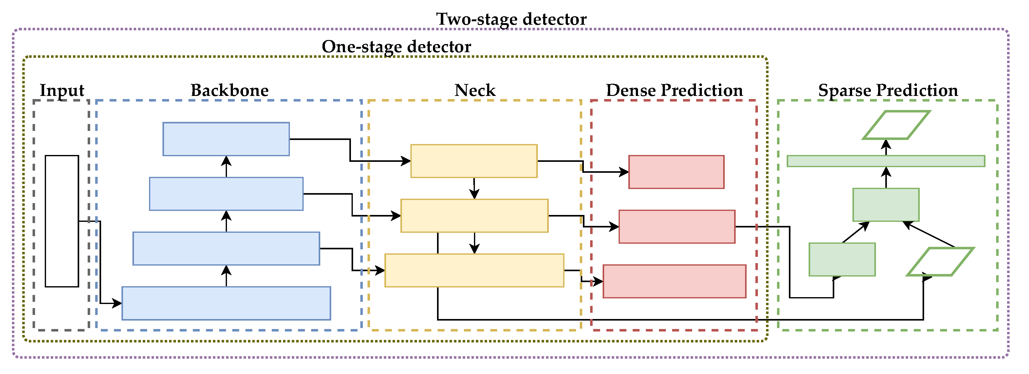
Object detection is one of the important tasks in image processing. Prior to 2012, object detection was usually performed with classical machine learning approaches. As discussed in Section 2, the object detection algorithms based on deep learning are classified into two large branches: one-stage detectors and two-stage detectors. The architecture of both object detection algorithms is shown in Figure 1.
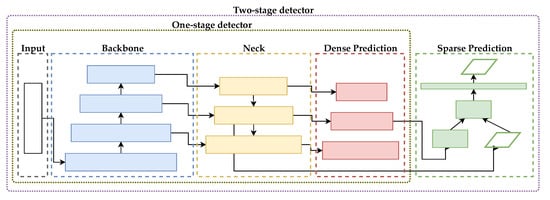
Figure 1.
One-stage and two-stage object detection algorithm.
We selected the best-performing one-stage and two-stage detectors to benchmark against our proposed model in this work. We selected Faster R-CNN [11] for two-stage detector, while YOLOv2, YOLOv2-Tiny, YOLOv3, YOLOv3-Tiny, YOLOv4, and YOLOv4-Tiny [13,14,15] for the one-stage detector.
3.1.1. Two-Stage Detector: Faster R-CNN
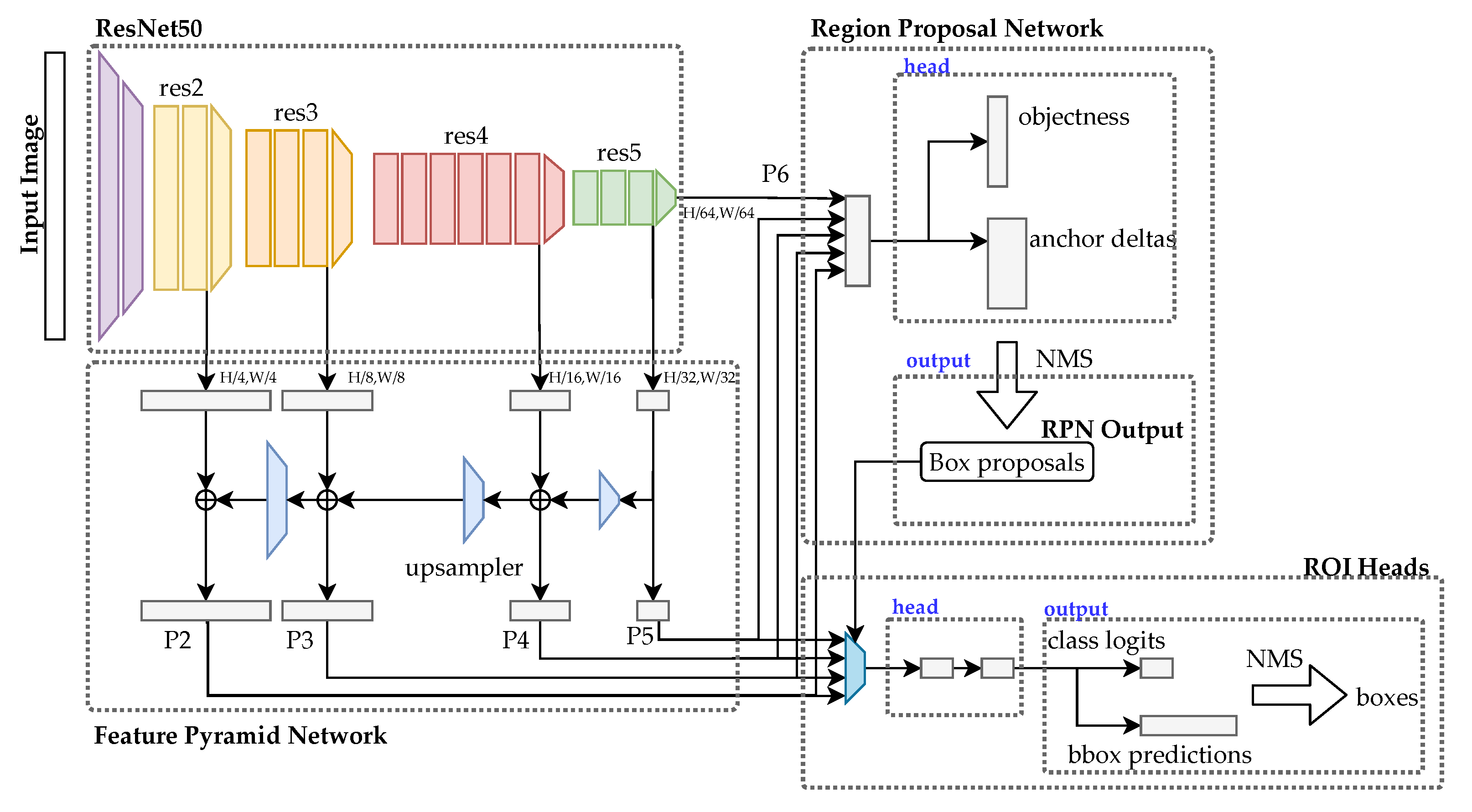
R-CNN [9] uses region proposals for object detection in an image. The region proposal is a rough guess of the object location. A fixed number of regions are extracted through a selective search. For every region proposal, a feature vector is extracted. Similar regions are merged together through the greedy algorithm, and candidate regions are obtained. Fast R-CNN [10] improves the approach by using a shared convolutional feature map generated directly from the input image to form a region of interest (RoI). Faster R-CNN [11] introduces a region proposal network (RPN) to predict the object bounding boxes and objectness score with little effect on the computational time. The architecture is shown in Figure 2.

Figure 2.
Faster R-CNN architecture.
Conceptually, Faster R-CNN comprises three components, namely the feature network, RPN, and detection network. The feature network is usually a state-of-the-art pretrained image classification model, such as VGG or ResNet, with stripped classification layers. It is used to collect features from the image. In this work, we used a feature pyramid network (FPN) with ResNet50. FPN combines low-resolution and semantically powerful features with high-resolution, but semantically weak features via a top-down pathway and lateral connections. The output of the FPN is then used for the RPN and ROI pooling. The RPN is a simple network with three convolutional layers. One common convolutional layer is fed into two layers for classification and bounding box regression. The RPN will then generate several bounding box proposals that have a high probability of containing objects. The detection network or the ROI head then considers the input from the FPN and RPN to generate the final class and bounding boxes.
3.1.2. One-Stage Detector: You Only Look Once
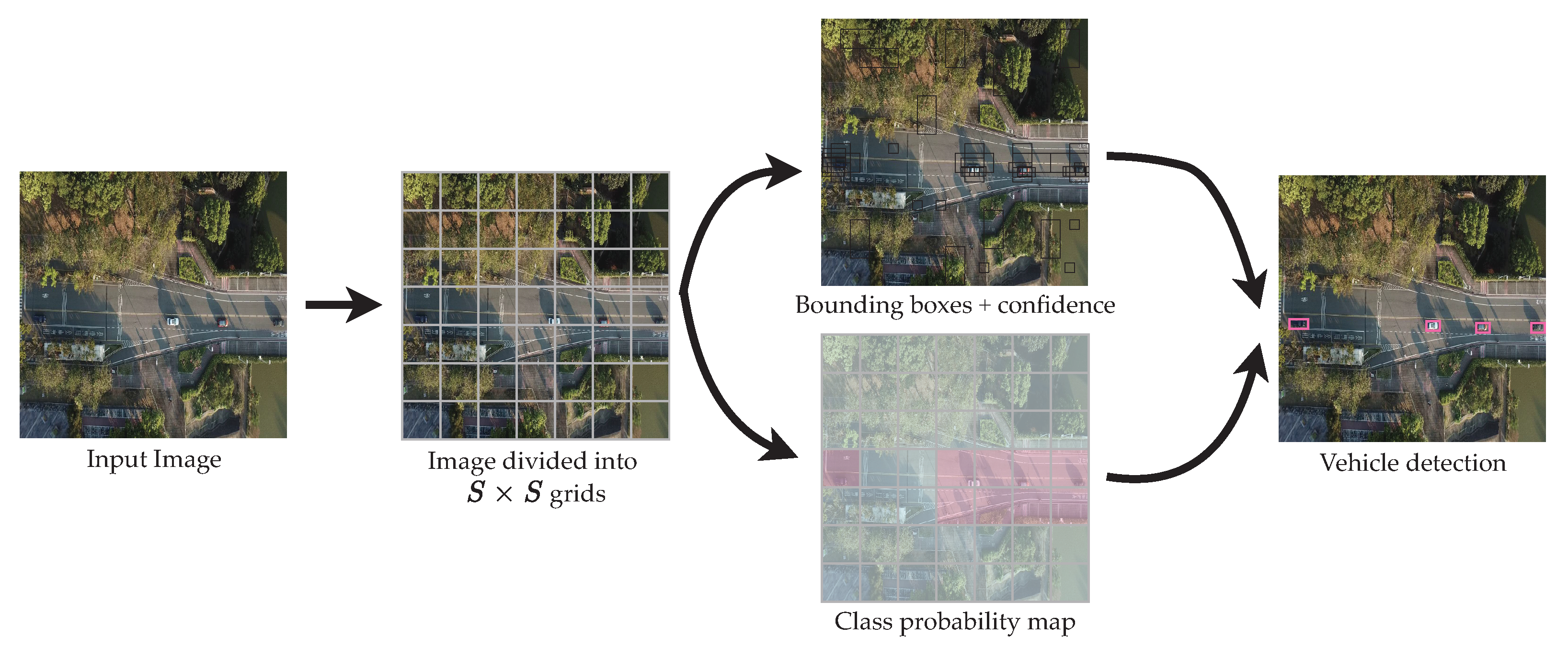
YOLO [12] predicts and classifies bounding boxes of objects in a single pass. Compared to Faster R-CNN, there is no region proposal phase. YOLO first splits an image into nonoverlapping grids. YOLO predicts the probability of a present object, the coordinates of the predicted box, and the object’s class for each cell in the grids. The network predicts B bounding boxes in each cell and the confidence scores of these boxes. Each bounding box carries five parameters, , where are the center of the predicted box, is the width and height of the box, and is the confidence score. Then, the network calculates the probabilities of the classes for each cell. The output of YOLO is , where C is the number of classes. The framework is shown in Figure 3. The first version of YOLO, coined YOLOv1, reportedly achieves a faster inference time, but lower accuracy compared to a single-shot detector (SSD) [16].
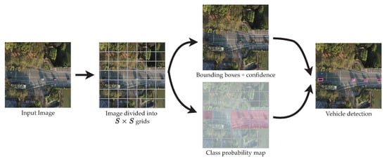
Figure 3.
YOLO model detection framework.
YOLO9000, or more commonly known as YOLOv2 [13], was proposed to improve the accuracy and detection speed. YOLOv2 uses convolutional layers without fully connected layers (Darknet-19) and introduces anchor boxes. Anchor boxes are predefined boxes of certain shapes to capture objects of different scales and aspects. The class probabilities are calculated at every anchor box instead of a cell, as in YOLOv1. YOLOv2 uses batch normalization (BN) and a high-resolution classifier, further boosting the accuracy of the network.
YOLOv3 [14] uses three detection levels rather than the one in YOLOv1 and YOLOv2. YOLOv3 predicts three box anchors for each cell instead of the five in YOLOv2. At the same time, the detection is performed on three levels of the searching grid (, , ) instead of one (), inspired by the feature pyramid network [62]. YOLOv3 introduces a deeper backbone network (Darknet-53) for extracting feature maps. Thus, the prediction is slower compared to YOLOv2 since more layers are introduced.
YOLOv4 [15] was introduced two years after YOLOv3. Many technical improvements were made in YOLOv4, while maintaining its computational efficiency. The improvements are grouped into bag of freebies (BoF) and bag of specials (BoS). In BoF, all improvements introduced did not affect the inference time. The authors implemented CutMix and mosaic data augmentation, DropBlock regularization, class label smoothing, complete IoU (CIoU) loss, cross mini-batch normalization (CmBN), self adversarial training (SAT), the cosine annealing scheduler, optimal hyperparameters through genetic algorithms, and multiple anchors for a single ground truth. On the other hand, BoS represents improvements that will affect the inference time slightly, but have a significant increase in accuracy. They include the Mish activation function, cross-stage partial (CSP) connections, the multi-input weighted residual connection (MiWRC), spatial pyramid pooling (SPP), the spatial attention module (SAM), the path aggregation network (PAN), and distance IoU loss (DIoU) in nonmaximum suppression (NMS). We refer the reader to the original article for more information.
This work considered six different YOLO models, which were YOLOv2, YOLOv2-Tiny, YOLOv3, YOLOv3-Tiny, YOLOv4, and YOLOv4-Tiny.
3.2. Proposed Model: YOLO-RTUAV
YOLOv4-Tiny was developed to simplify the YOLOv4 network, allowing the network to run on low-end hardware. The model only contains a two-layer output network. Therefore, YOLOv4-Tiny has ten-times fewer parameters than YOLOv4. However, it is not able to detect a multiscale object and missing detection with overlapped objects. As for aerial images, objects are usually small in size, yet occluded by surrounding items such as trees and buildings. Therefore, an improved YOLOv4-Tiny in terms of detection accuracy, inference speed, and model size is required.
To solve the problems raised above, an improved YOLOv4-Tiny is proposed, coined YOLO-RTUAV. Our proposed model is shown in Figure 4. The proposed YOLO-RTUAV network should achieve three objectives:
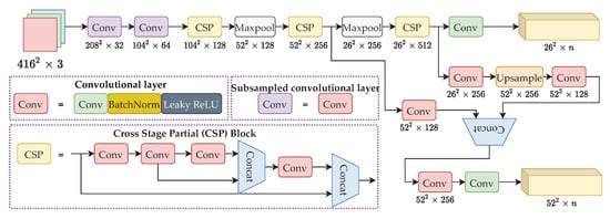
Figure 4.
The YOLO-RTUAV model architecture. n is calculated such that .
- Detect small objects in aerial images;
- Efficient, yet accurate for real-time detection in low-end hardware;
- Small in size and reduced in parameters.
The main improvements of our proposed model are summarized below:
- Changing the output network to a larger size, allowing smaller objects to be detected;
- Usage of Leaky ReLU over the Mish activation function [63] in the convolutional layers to reduce the inference time. The backbone remains the same as the original YOLOv4-Tiny, which is CSPDarknet-19;
- Usage of several convolutional layers to reduce the complexity of the models;
- DIoU-NMS is used to reduce suppression error and lower the occurrence of missed detection;
- Complete IoU loss is used to accelerate the training of the model and improve the detection accuracy;
- Mosaic data augmentation is used to reduce overfitting and allows the model to identify smaller-scale objects better.
Firstly, the detection layer size is changed to detect smaller objects. The detection layer remains two layers, with the output size of replaced with . YOLOv4-Tiny can detect objects in a wide range of natural image objects, but cannot detect small objects in aerial images. Therefore, the highly subsampled layers are not necessary, whereby we removed the coarse detection level layer of size and replaced it with a finer detection level layer of size . Given an input image of size , the detection layer is suitable for medium-scale object detection, and the detection layer is suitable for small-scale object detection. Therefore, the proposed YOLO-RTUAV can realize smaller object detection, which is critical for aerial images.
The backbone of our proposed model is CSPDarknet-19. In contrast to YOLOv4’s CSPDarknet-53, CSPDarknet-19 has gradually reduced the number of parameters while not hurting the accuracy significantly. The cross-stage partial (CSP) module divides the feature map into two parts and combines the two parts by the cross-stage residual edge, as illustrated in Figure 4. The CSP module allows gradient flow to propagate in two different paths, increasing the correlation difference of gradient information. Therefore, the network can learn significantly better than residual blocks. To further reduce the inference time, the Mish activation layer is not used in our proposed model. Instead, Leaky ReLU is used since the calculation was not complex, requiring less computational time.
Since the second YOLO output layer is calculated from the second and third CSP layer, which has a mismatch in channel size and output shape, naively, one would use convolutional layers to match the channel size. Therefore, the agreed channel size is then 512. This, however, requires large computation when the last convolutional layer is dealing with a large channel size. To solve this issue, we first used two convolutional layers before concatenation, agreeing on the channel size to be 256. Thus, the computation needed is smaller, with no effect on detection accuracy. A further explanation is available in Appendix A.
The most commonly used nonmaximum suppression (NMS) technique is Greedy NMS, a greedy iterative procedure. Although Greedy NMS is relatively fast, it comes with several pitfalls. It suppresses everything within the neighborhood with lower confidence, keeps only the detection with the highest confidence, and returns all the bounding boxes that are not suppressed. Therefore, Greedy NMS is not optimal in this work since the objects in the dataset are usually small and overlapped objects tend to be filtered out. To address the issue, DIoU-NMS [64] was used. DIoU-NMS considers both the overlapping areas and the distance between the center points between the two borders. Thus, it can effectively optimize the process of suppressing redundant bounding boxes and reducing missed detections. The definition of DIoU-NMS is shown in Equation (1).
where denotes the distance of the center points of the two boxes, is the classification score, and is the NMS threshold. Equation (1) compares the distance of the prediction box of the highest score with the i-th box, . If the differences between and exceeds , the score remains, otherwise it is filtered out.
The complete intersection over union (CIoU) loss function is deployed for bounding box regression. CIoU has proven to improve accuracy and accelerate the training process. Usually, the objective loss function for YOLO models is the sum of bounding box loss, confidence loss, and classification loss. The bounding box regression loss function is applied to calculate the difference between the predicted and ground truth bounding boxes. The common metric to calculate the bounding box regression is the intersection over union (IoU). The IoU is used to measure the overlapping ratio between the detected bounding box, , and the ground truth bounding box, , as shown in Equation (2).
The IoU loss is then calculated as shown in Equation (3).
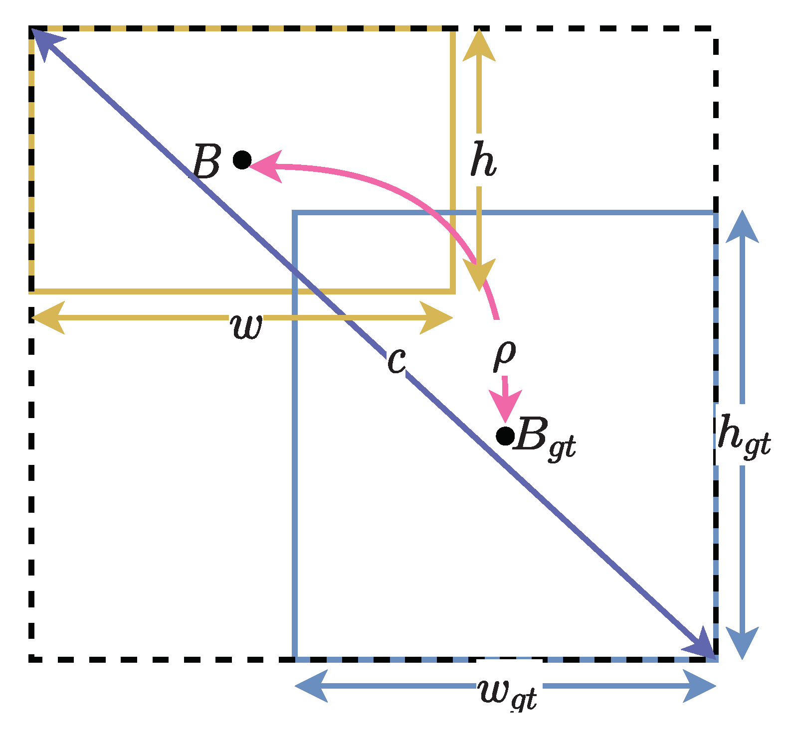
IoU loss suffers from a lower decrease rate during training. When there is no intersection between the ground truth and predicted box, the IoU is zero. Therefore, IoU loss does not exist. This renders the inability of the loss function to reflect the distance between the ground truth and the predicted box. Therefore, CIoU loss is used to overcome the stated issue. The CIoU uses the distance between the predicted and ground truth bounding box center point and compares the aspect ratio between the ground truth and predicted bounding box. The formula is shown in Equation (4). Figure 5 illustrates the calculation of the CIoU.
where is the Euclidean distance, c is the diagonal length of the smallest enclosing box covering the two boxes, and is a positive tradeoff parameter, denoted as . v measures the consistency of aspect ratio, , where w and h represent the width and height of the box, respectively.

Figure 5.
CIoU calculation conceptualized.
The classification function, , only penalizes if the object is present in the grid cell. It also penalizes the bounding box coordinate if that box is responsible for the ground box (highest IOU). It is calculated as shown in Equation (5),
The confidence loss, , is calculate such that,
The total loss function in our proposed model is the same as YOLOv4. The loss function comprises three parts: classification loss (), regression loss (), and confidence loss (). The loss is therefore calculated as shown in Equation (7).
where is the grids generating B candidate boxes. Each candidate box will obtain the corresponding bounding boxes through the network and form bounding boxes. If no objects are detected in the box (), only the confidence loss of the box is calculated. Cross-entropy error is used to calculate the confidence loss and is divided into (object) and (no object). The weight coefficient, , is used to reduce the weight of the loss function. As for classification loss, cross-entropy error is used. The j-th anchor box of the i-th grid is responsible for the given ground truth, then the bounding box generated by this anchor box will calculate the classification loss function.
Furthermore, we utilized mosaic data augmentation while training the model. This combines four training images into one with certain ratios. This technique allows the model to identify objects of a smaller scale. It also encourages the model to localize different types of images in different portions of the frame. A sample of images that have undergone mosaic data augmentation is shown in Figure 6.

Figure 6.
Example of mosaic data augmentation images from the VAID dataset [23].
We compare our proposed models with the original YOLO models in Table 1. It is observed that all the greatness of YOLOv4-Tiny remains while the number of layers is reduced. Since some of the layers are removed, the model size is smaller as well.

Table 1.
Characteristics of various YOLO models.
4. Experiment Settings
4.1. Dataset Description
This paper utilized two datasets, namely the Vehicle Aerial Imaging from Drone (VAID) dataset [23] and the Cars Overhead With Context (COWC) dataset [24].
4.1.1. VAID Dataset
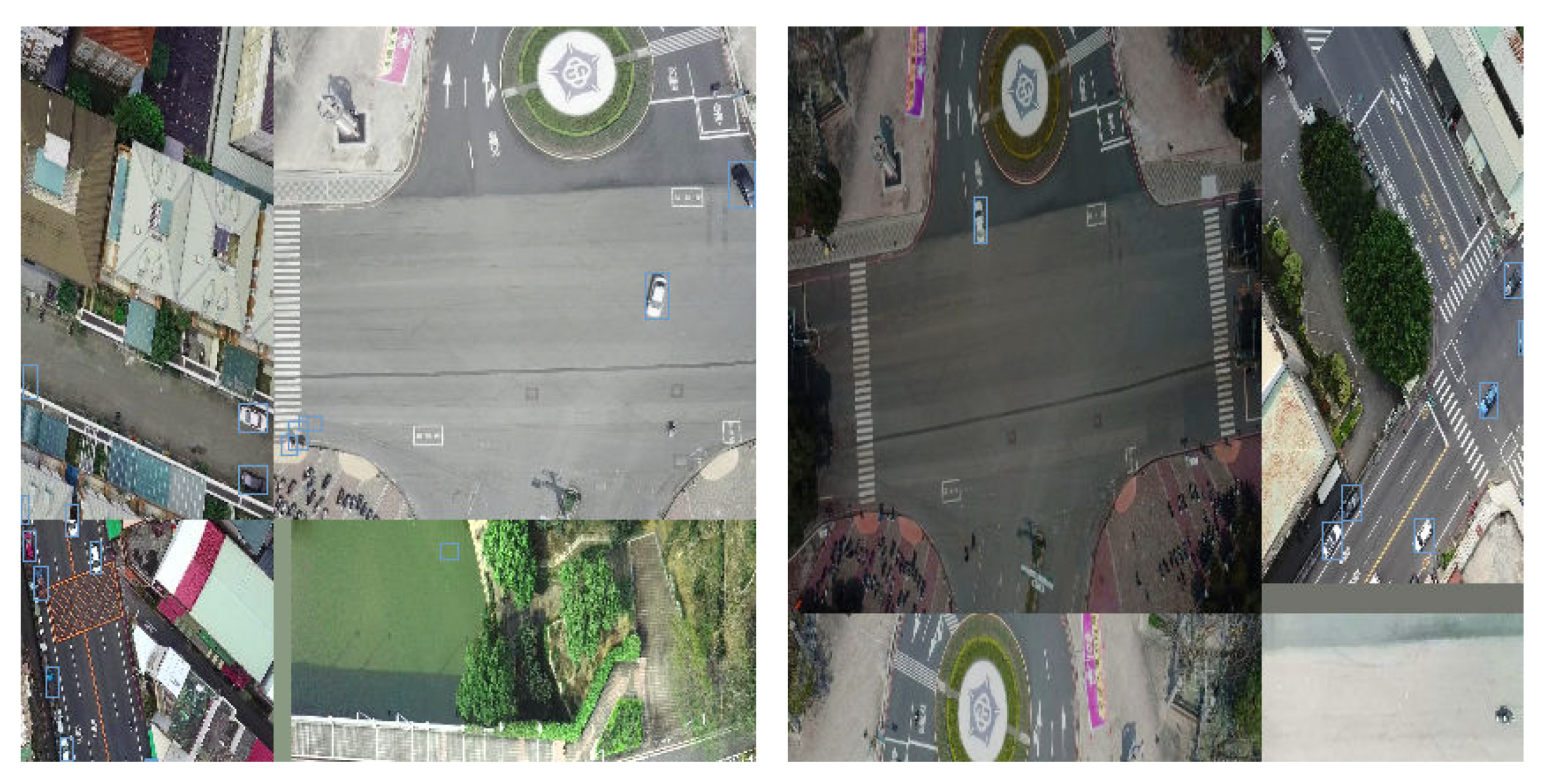
This dataset contains 5985 images with varied illumination conditions and viewing angles, collected at different places in Taiwan. It contains seven classes, and the ratio of the training, validation, and testing datasets was set as 70:20:10. The number of objects in each class is shown in Table 2. The images have a resolution of px in JPG format. Samples of the images are shown in Figure 7.
Table 2.
Training, validation, and testing split for the VAID dataset.

Figure 7.
Sample images from the VAID dataset with annotated classes.
4.1.2. COWC Dataset
This dataset comprises several high-resolution RGB and grayscale images captured at different locations (Columbus of size , Potsdam of size , Selwyn of size ). We used the updated dataset, named COWC-M, where the authors further divided the dataset into four vehicle classes instead of only one main class. The authors patched the images in the dataset with the size of . For example, a single image of size was divided into 49 patches. The images were then further divided into training, validation, and testing with the ratio of 80:10:10. The number of objects in each set is shown in Table 3. The patches of a single image were split into the training, validation, and testing set randomly. Samples of the image patches are shown in Figure 8.
Table 3.
Training, validation, and testing split for the COWC dataset.

Figure 8.
Illustration of obtaining image patches of size from a large image in the COWC dataset.
Table 4 summarizes the datasets used in our experiments.
Table 4.
Datasets used in this study.
4.2. Experimental Setup
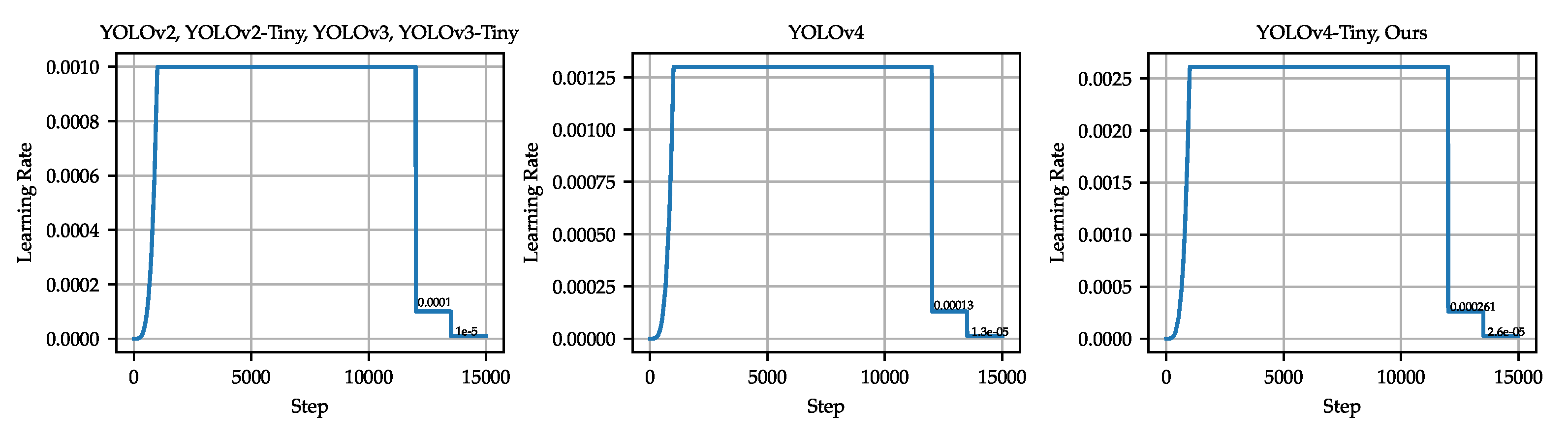
The framework used to train Faster R-CNN was Detectron 2 [65], with the configuration file named faster_rcnn_R_50_FPN_3x.yaml. The model was trained with 15,000 epochs, with 1000 linear warmup iterations. The training rate was reduced at 12,000 and 13,500 epochs. The initial training rate was set to 0.001. The learning rate is shown in Figure 9. The batch size was set to 4. We kept the default values for the momentum (0.9) and weight decay (0.0001).
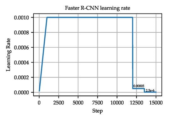
Figure 9.
The scheduled learning rate used to train the Faster R-CNN models.
As for YOLO and our proposed model, the framework used to train the models was Darknet. The model was trained with 15,000 epochs, with 1000 exponential warmup iterations according to . The training rate was reduced at 12,000 and 13,500 epochs. The initial training rate was set to 0.001, 0.0013, and 0.00261 for different YOLO models and is shown in Figure 10. We kept the default values for the momentum (0.949) and weight decay (0.0005) for YOLOv4, while all other models were set to a momentum of 0.9 and a weight decay of 0.0005.
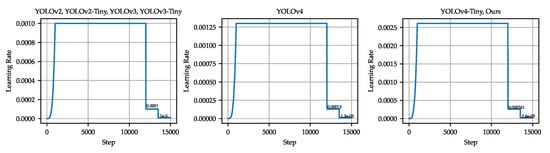
Figure 10.
The scheduled learning rate used to train the YOLO models.
The anchor boxes used in all the models are shown in Table 5. Our proposed model’s anchor box sizes were the same as YOLOv4-Tiny, since our initial search for optimum anchor box sizes had almost a similar set as YOLOv4-Tiny. Note that choosing a large number of prior boxes will produce greater overlap between anchor boxes and bounding boxes. However, as we increase the number of anchor boxes, the number of convolution filters in prediction filters increase linearly, which will result in a large network size and increased training time. For each models, three different input sizes (, , and ) were considered and trained.
Table 5.
Anchor box sizes for different models.
All of the models were trained with the Nvidia Tesla T4 or Nvidia Quadro P5000 GPUs. The trained models were then supplied to two powerful hardware, Nvidia Tesla T4 and Nvidia Quadro P5000, and one edge hardware, Nvidia Jetson Nano 2 GB, to calculate the inference time.
4.3. Evaluation Criteria and Metrics
The following criteria were used to evaluate and compare the various models:
- The IoU measuring the overlap between the predicted and the ground truth bounding boxes, as discussed in Equation (2);
- The main evaluation metric used in evaluating object detection models is mAP. mAP provides a general overview of the performance of the trained model. A higher mAP represents better detection performance. Equation (8) shows how mAP is calculated;where is the average precision for the i-th class and C is the total number of classes. corresponds to the area under the PR curve and is calculated as shown in Equation (9):where and is the recall ratio and precision ratio when the n-th threshold is set. Usually, and represents the AP (single class) calculated with the IoU set as 0.5 and 0.75, respectively. is the average value of AP with the IoU ranging from 0.5 to 0.95 with a step of 0.05. , , and , on the other hand, represent the average APs of all classes at different settings of the IoU;
- Besides mean average precision (mAP), precision, recall, and the F1-score are also common criteria for model evaluation. The computations are as follows:where , , and represent true positive, false positive, and false negative, respectively;
- The precision–recall curve (PR curve) plots the precision against the recall rate. As the confidence index is set to a smaller value, the recall increases, signaling more objects to be detected, while the precision decreases since false positive objects increase. The PR curve is useful to visualize the performance of a trained model. A perfect score would be at , where both precision and recall is at 1. Therefore, if a curve bows towards , the model performs very well;
- Number of frames per second (FPS) and inference time (in milliseconds) to measure the processing speed.
5. Results and Discussion
The detection performance for each dataset (VAID and COWC) is evaluated and discussed in this section. We trained the datasets with three different input sizes (, , and ) for all detectors. The results of each detector are tabulated, and the precision–recall curve is plotted. Besides, we provide the inference time collected on different hardware. Then, we provide a general discussion of the performances of both datasets.
5.1. VAID Dataset
The detection results of the different models are shown in Table 6. We performed experiments on three different input sizes (, , and ), and the individual classes performance was recorded. We remind that the vehicle size of the objects in the images is usually px, as shown in Table 4.
Table 6.
Detection result on the VAID dataset. The individual class results are their respective . Numbers in red, blue, and green represent the best results for the input sizes of , , and , respectively.
From Table 6, it is observed that a larger input size would increase the detection accuracy. YOLOv2 and YOLOv2-Tiny provided the lowest detection accuracy among all. For the input size of , the best result was given by YOLOv4 (), followed by YOLOv3 () and our proposed model (). For the input size of , the best result was given by YOLOv4 (), followed by YOLOv3 () and our proposed model (). For the input size of , the best result was given by YOLOv4 (), followed by YOLOv3 () and our proposed model (). When comparing with the tiny versions of the YOLO models (YOLOv4-Tiny, YOLOv3-Tiny, and YOLOv2-Tiny), we observed that our model led in terms of detection accuracy. Our proposed model achieved similar or better results than YOLOv4-Tiny in all three input sizes. Our model always achieved higher precision than the other models (except for the input size of ), revealing that it can reduce the number of false positives. Regarding detection accuracy on individual classes, we found that almost all classes had significant improvement over YOLOv4-Tiny, with an increase in accuracy within 1–4%. This was due to the added finer YOLO detection head, where it can effectively detect smaller objects. Interestingly, we observed that our model performed better than YOLOv4 for the “bus” object with the input size of .
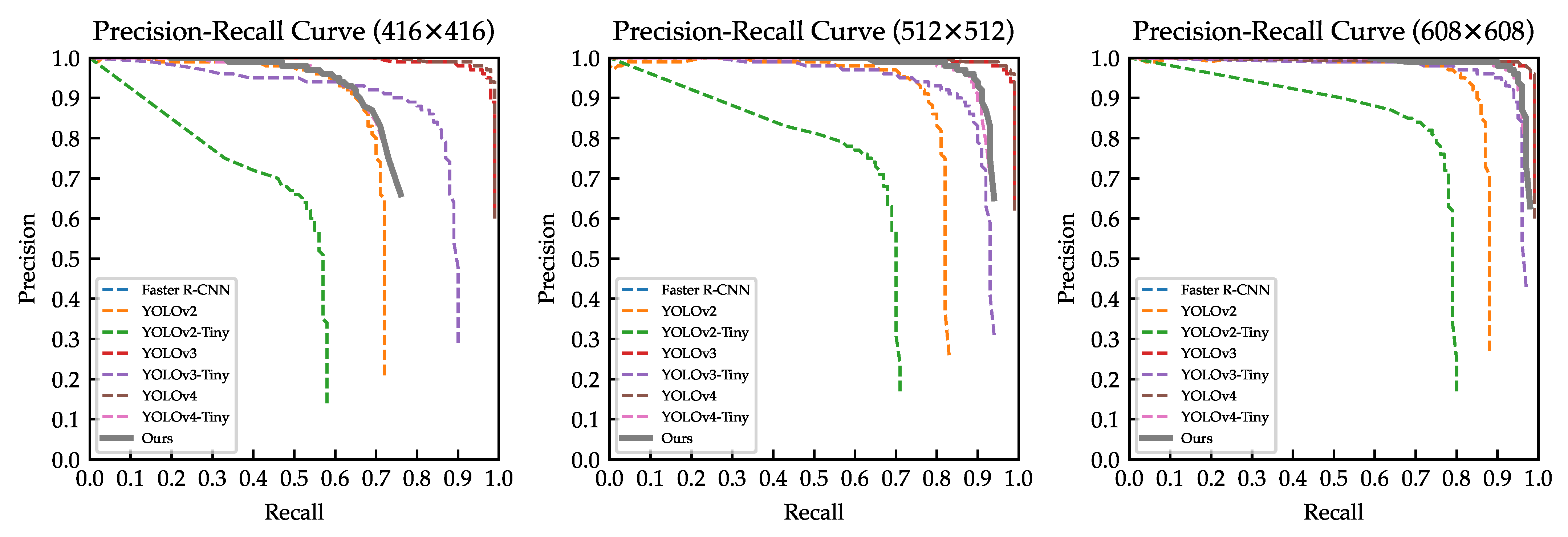
Figure 11 shows the precision–recall curve for all models of various input sizes. It was confirmed that our model outperformed almost all models, except YOLOv4 and YOLOv3. Our model provided a good behavior of the precision–recall balance, as illustrated in Figure 11.
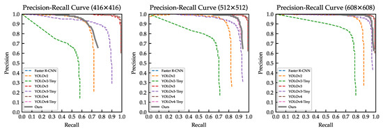
Figure 11.
Precision–recall curve for all models trained on the VAID dataset.
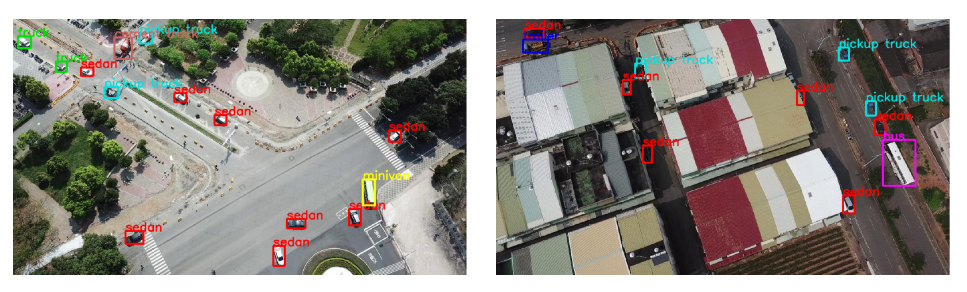
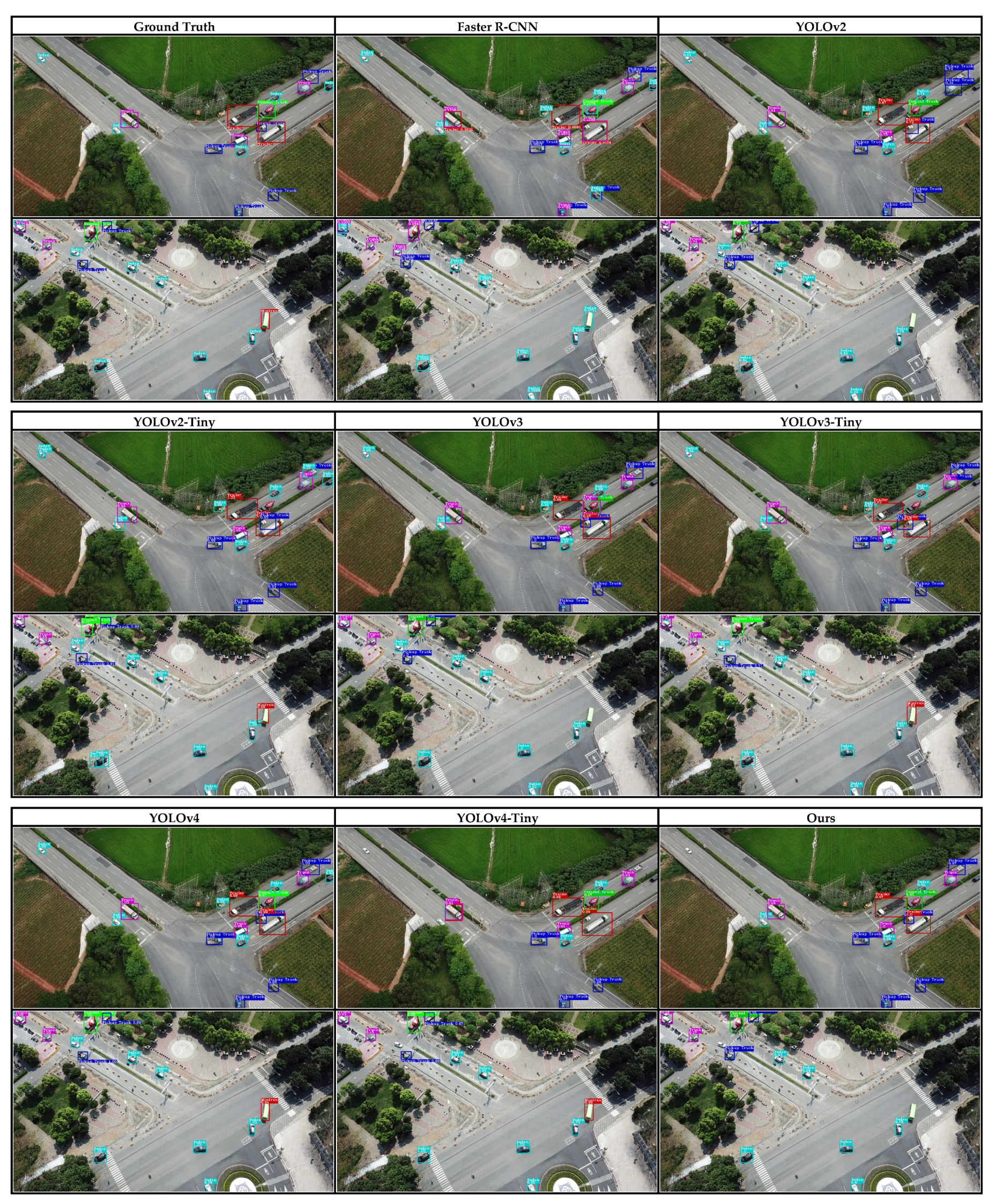
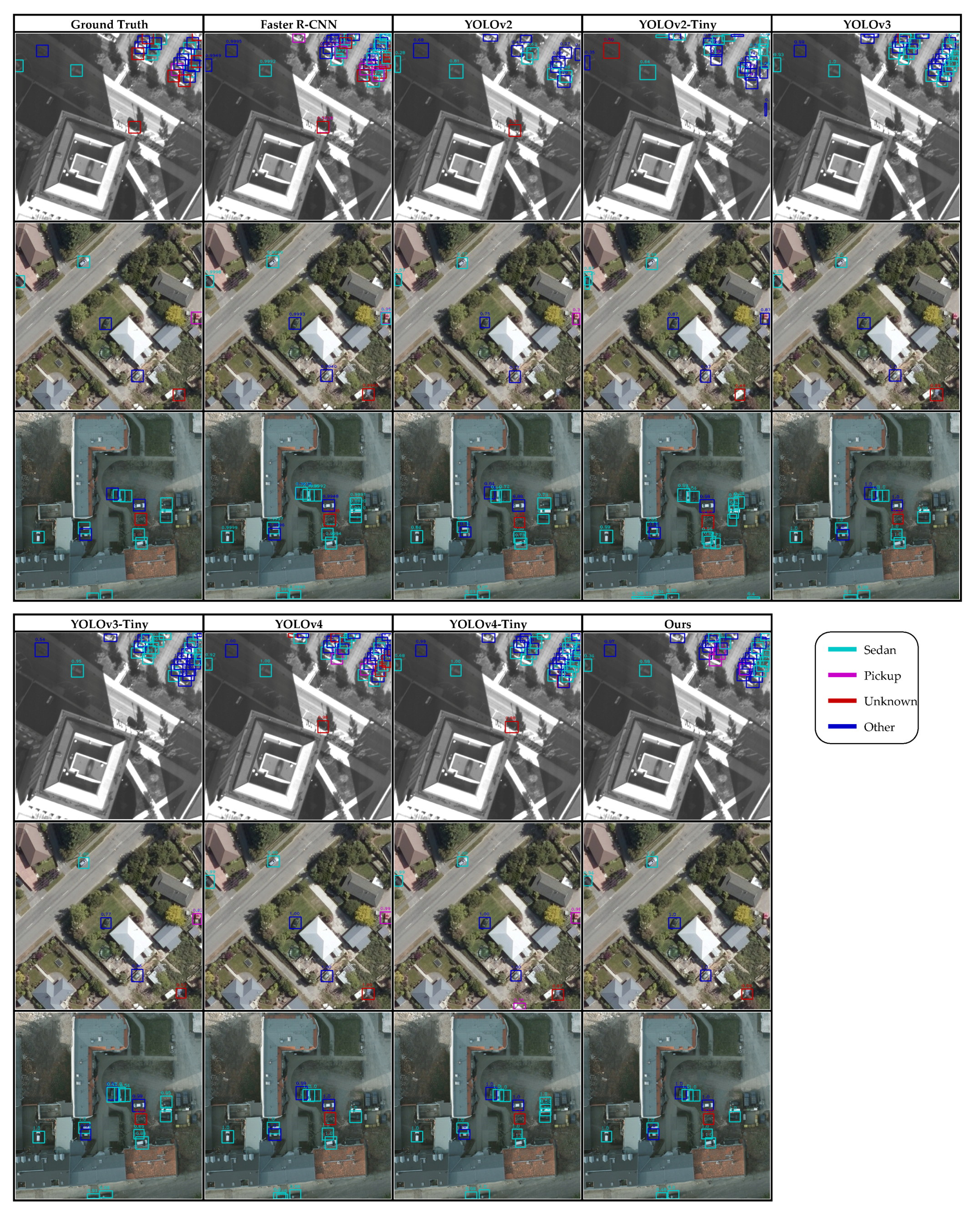
The detection results of the various detectors are shown in Figure 12. We took two sample frames from the test set and the inference on all detectors. We selected the frame that had the most classes of objects. There are two small “sedans” on the top left corner and top right corner in the first row of the figure. Besides, there is an occluded “pickup truck” at the bottom right corner. These three objects are the key to differentiate the effectiveness of different detectors. We observed that Faster R-CNN, YOLOv2-Tiny, and YOLOv4 successfully located all the objects. However, Faster R-CNN and YOLOv2-Tiny misclassified some objects, while YOLOv4 classified all the objects correctly with a high level of confidence. Other detectors failed to locate one or two of the small objects, as described before. As for our proposed model, it failed to identify the “sedan” on both the top left corner and top right corner. A similar detection was observed in YOLOv4-Tiny, except that our model produced a detection with a higher level of confidence. Compared to Faster R-CNN, our model did not have multiple bounding boxes on a single object, signaling that the NMS was working as intended. For the image in the second row, there is much background noise, where trees and parks are the main noise that could confuse the models. It was observed that Faster R-CNN was confused with “cement truck” and “truck”. Compared to the first image, Faster R-CNN produced less classification error, and no stacking of the bounding box was observed. As for our model, it did not classify the minivan, while other objects were detected and classified correctly.

Figure 12.
Detection results of various detectors (input size of ) on the VAID dataset.
Table 7 shows an in-depth exploration of our models in terms of the computational efficiency.
Table 7.
Comparison in terms of the model size, computational requirements, and inference time on different hardware for input size of for the VAID dataset. The number in bold denotes the best result.
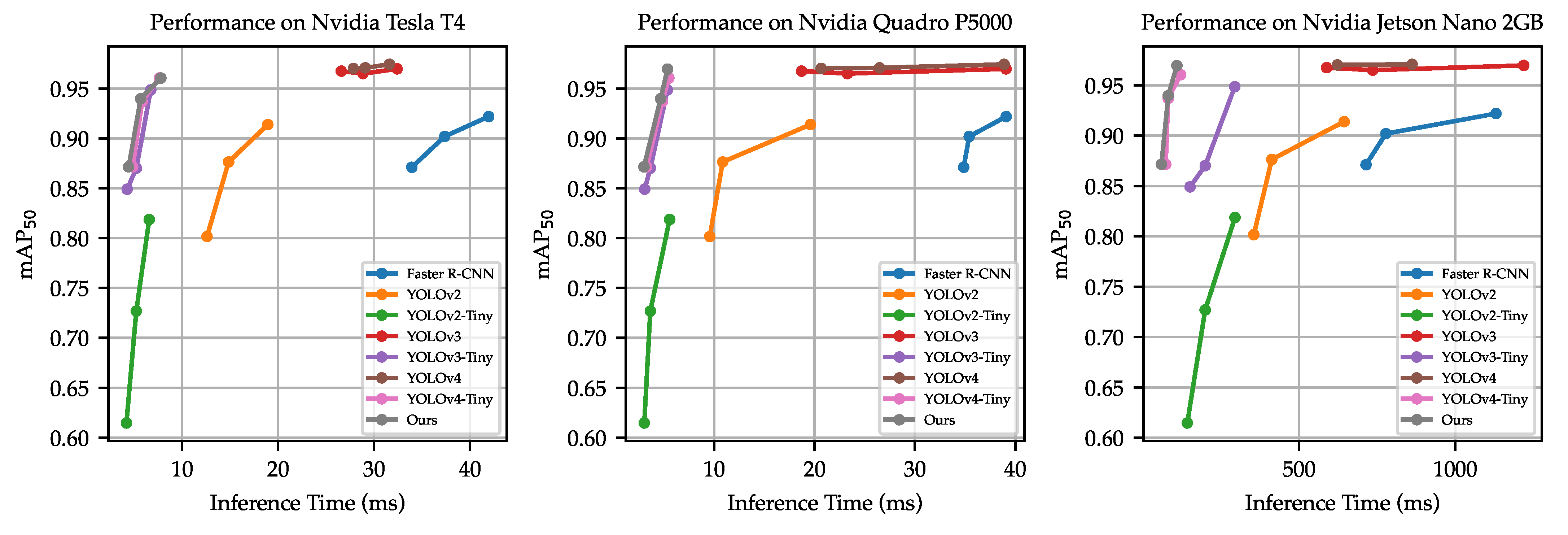
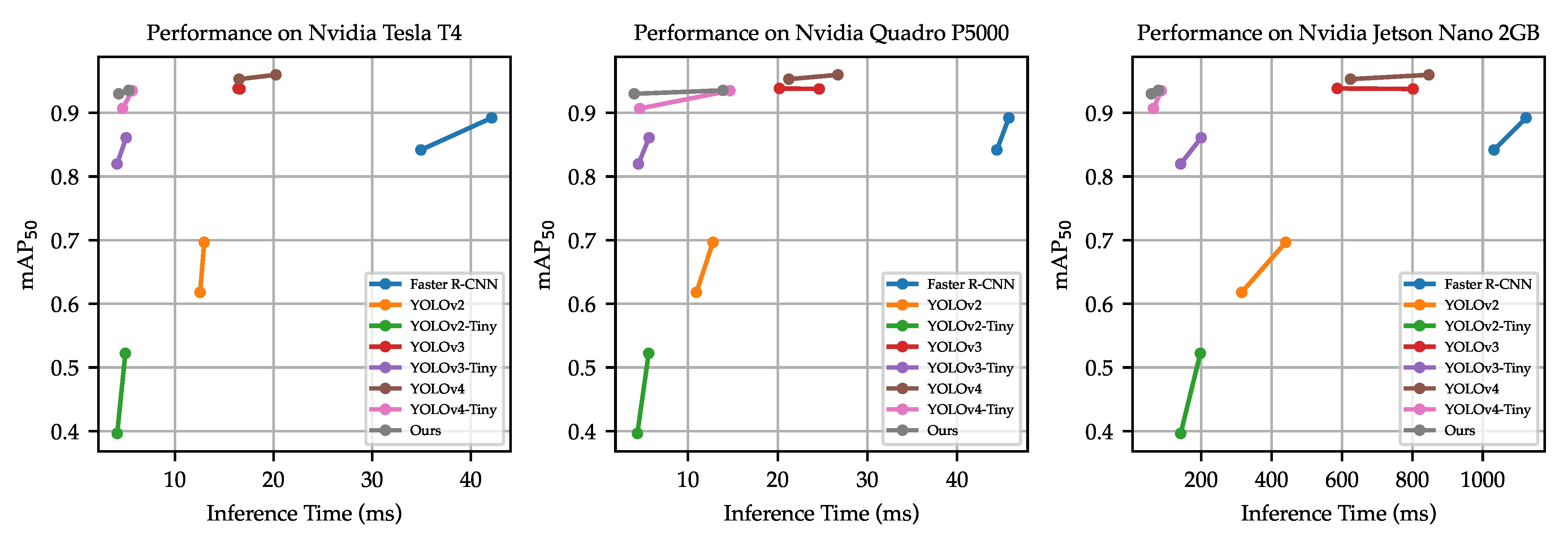
As observed in Table 7, even though our proposed model took a little bit longer than YOLOv2-Tiny, YOLOv3-Tiny, and YOLOv4-Tiny on the Tesla T4 and Quadro P5000 and the model size and number of parameters were smaller, mAP was higher than them. In terms of edge hardware inferencing, our model could achieve around an 81 ms inference time on the Jetson Nano, thanks to its relatively small floating-point operations (FLOPs).
The mAP versus inference time plot is shown in Figure 13. It is observed that our model used almost the same inference time, but achieved slightly higher detection accuracy than YOLOv4-Tiny.
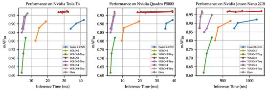
Figure 13.
Performance of various detectors on the Tesla T4, Quadro P5000, and Jetson Nano 2 GB. The graph is plotted with the inference time collected from both input sizes of and for all detectors. Note that YOLOv4 with the input size of failed to run on the Nvidia Jetson Nano 2 GB.
5.2. COWC Dataset
The second dataset used in our study was the COWC dataset. Table 8 provides the detection results on various models trained on two different input sizes, namely and .
Table 8.
Detection results on the COWC dataset. Numbers in blue and red represent the best result for input sizes of and respectively.
From Table 8, it is observed that YOLOv4 topped the for both input sizes of and . YOLOv3 came in second, and our proposed model came in third in terms of . In terms of precision, YOLOv3 achieved the highest precision among all, followed by our model and YOLOv4. This is different from the VAID dataset, where our proposed model topped in terms of precision. This was mainly due to the dataset used, where COWC seems to have objects with a larger size () than VAID (). Recall that we replaced the YOLO output with a larger size to accommodate the finer detection of smaller sizes; therefore, our model was not able to capture the slightly larger objects well. When comparing the tiny version of YOLO, our model topped in terms of almost all metrics. Our model achieved the highest , precision, and F1 score. Faster R-CNN provided lower detection accuracy since it was not designed to detect small objects. Even though the anchor size was adapted according to the training set, they were not built to detect small objects and could not yield good detection results. As for individual class , we observed that our model outperformed the others for the “sedan” class for the input size of , thus revealing that our model could detect smaller objects in the image since the only class in the dataset with a consistently small object size was “sedan”. Note that the size of the “sedan” in this dataset was smaller than the other classes. As for other objects, YOLOv4 yielded the highest detection accuracy. When comparing with YOLOv4-Tiny, our model outperformed it in almost all classes. In short, YOLOv4 strikes for higher detection accuracy, YOLOv3 for precision detection, and our proposed model for the balance between detection accuracy and inference time.
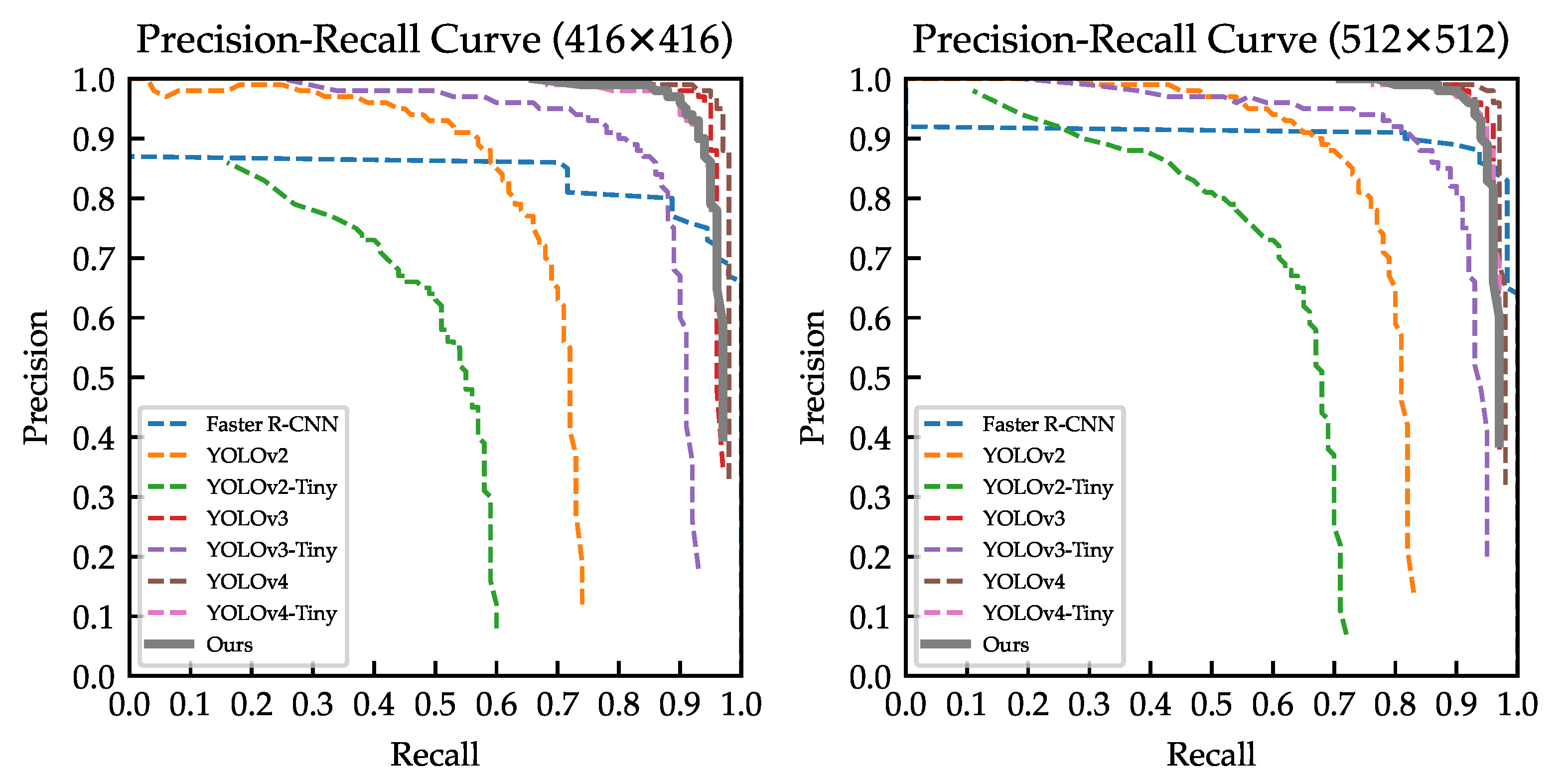
We provide the precision–recall curve for all the models in Figure 14. We can once again confirm that our model outperformed almost all models, except the huge YOLOv4 and YOLOv3.
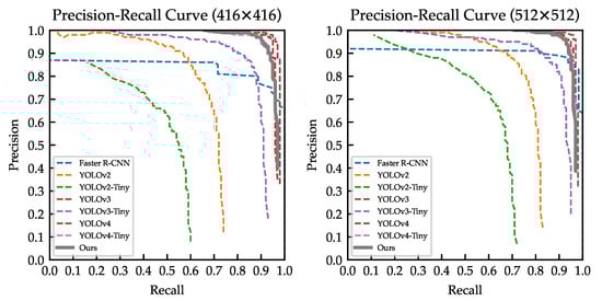
Figure 14.
Precision-recall curve for all models trained on the COWC dataset.
The detection results of the various detector are illustrated in Figure 15. We took three sample frames from the test set and inference on all the trained detectors of input size . As shown in the first row, the image is partially occluded with four objects that are “hidden” in the shadow and contains multiple objects in the upper right corner. Our model only detected three out of four occluded objects, while YOLOv4-Tiny successfully detected all four occluded objects. As for the upper right corner section, it was observed that Faster R-CNN generated many bounding boxes, but did not classify most of the boxes correctly. The NMS in our model successfully suppressed many unwanted bounding boxes and was able to classify most of the objects correctly. Compared to YOLOv4 and YOLOv4-Tiny, our model could identify the classes more accurately. In the second and third rows, almost all models could detect and classify the object correctly. It was observed that Faster R-CNN, YOLOv3, YOLOv4, and our model correctly classified most of the objects with high confidence.
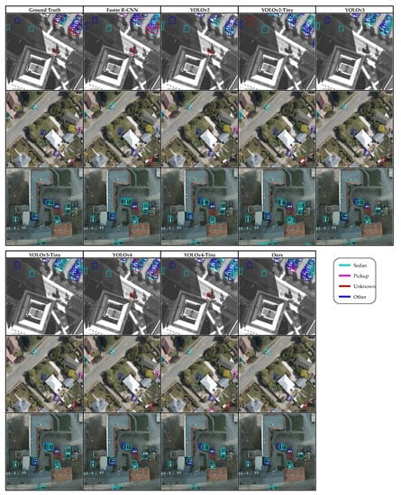
Figure 15.
Detection results of various detectors (input size of ) on the COWC dataset.
Our model was designed to strike a balance between detection accuracy and inference speed. In Table 9, we report the comparison between our proposed model against all other models of input size on the Tesla T4, Quadro P5000, and Jetson Nano in terms of the model size, billion floating-point operations (BFLOPs), number of parameters, inference time, and FPS. Our proposed model consumed the lowest disk space, with a model size of only 5.5 MB, only 23% of YOLOv4-Tiny. Our model required the lowest computational resource, coming in with only 7.73 BFLOPs and 1.43 M parameters. The detection accuracy was ranked second after the huge YOLOv4. In terms of inference time, YOLOv2-Tiny and YOLOv3-Tiny took a shorter time to perform inference on the Tesla T4 and Quadro P5000. However, the critical study of this work was to run inference on low-cost embedded hardware. We used the Jetson Nano 2 GB as our low-cost embedded hardware, whereby we observed that our model took the lowest time to compute, which took only 78.33 ms, equivalent to around 13 FPS. With 13 FPS, near-real-time results were obtained. We include the detection accuracy vs. inference time graph for all three GPUs in Figure 16.
Table 9.
Comparison in terms of the model size, computational requirements, and inference time on different hardware for the input size of for the COWC dataset. The number in bold represents the best result.
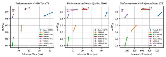
Figure 16.
Performance of various detectors on the Tesla T4, Quadro P5000, and Jetson Nano 2 GB. The graph is plotted with the inference time collected from both input sizes of and for all detectors.
From both of the experiments, we can conclude that our model struck a balance between detection accuracy and inference speed. Our model outperformed YOLOv4-Tiny on both of the datasets, despite requiring only 5.5 MB of storage to store the model. This is particularly useful when deploying on edge devices, where storage and processing power are usually the constraint. Apart from that, with the reduction of the FLOPs, we saw a minimal affect on the detection accuracy. An in-depth ablation study and our design of the proposed model is available in Appendix A.
We observed that for both datasets suffering from class imbalance (“minivan” and “cement truck” in the VAID dataset and “pickup” in COWC), YOLOv4, YOLOv4-Tiny, and our proposed model could still achieve competitive , while other models did not perform any better. Even though we tried to include augmentation to increase the number of objects for severely under-represented classes, their results stayed almost the same, since augmentation increased the objects in the classes; however, there was still a lack of representative features of the targeted classes. A possible way to solve this issue is through a resampling process, oversampling infrequent classes from the minority classes to match the quantity of the majority classes. However, we did not explore this as YOLOv4, YOLOv4-Tiny, and our proposed model did not suffer from lower on minority classes’ prediction.
6. Conclusions
We proposed an improved version of a one-stage detector, coined YOLO-RTUAV, to detect small objects in aerial images in this work. Our model was built based on YOLOv4-Tiny, specifically aimed at near-real-time inference of small objects on edge devices. Essentially, our model is lightweight with only 5.5 MB, and experiments on the Jetson Nano 2 GB showed the ability to achieve up to 13 FPS for an input size of . Experiments conducted on two datasets, namely VAID and COWC, illustrated that our proposed model outperformed YOLOv4-Tiny in terms of inference time and accuracy. Our model did not perform better than the more complicated YOLOv4. However, we believe that our model struck a balance between accuracy and inference time.
While YOLO-RTUAV provided promising results for the datasets used, some issues still exist and call for further research. Firstly, YOLO-RTUAV only focuses on small objects in aerial images. The performance on medium and large objects remains unknown since the datasets used mainly contain small objects. YOLO-RTUAV is not suitable for objects with a wide range of sizes. This bottleneck is solvable with the help of more YOLO layers with various output sizes, but it comes with the cost of more computational power requirements. Secondly, our experiment on the COWC dataset showed that our model can deal with RGB and grayscale images, and objects occluded by shadows remained detectable. However, such an assumption is limited to the COWC dataset, and more experiments are required to validate our claim. Therefore, datasets with different occlusions and background noise in the training and test datasets should be considered in future work. Thirdly, the reduction of the parameters using a convolutional layer showed a slight decrease in the detection accuracy. It would be interesting to explore other techniques, which reduce the model complexity, but retain the same detection accuracy. Finally, YOLO models are highly dependent on anchor boxes to produce predictions. This is a known problem whereby, to achieve optimum detection accuracy, a clustering analysis is required to determine a set of optimum anchors before model training. In addition, the usage of anchors increases the complexity of the detection heads. We suggest exploring the possibility of anchor-free prediction, such as YOLOX [66].
Author Contributions
Conceptualization, H.V.K. and J.H.C.; methodology, H.V.K. and Y.-L.C.; software, H.V.K. and K.K.Y.; validation, H.V.K., J.H.C., and C.-O.C.; formal analysis, H.V.K. and J.H.C.; investigation, H.V.K. and C.-O.C.; resources, H.V.K., J.H.C. and K.K.Y.; data curation, H.V.K.; writing—original draft preparation, H.V.K.; writing—review and editing, H.V.K., J.H.C., C.-O.C. and Y.-L.C.; visualization, H.V.K.; supervision, J.H.C. and C.-O.C.; project administration, J.H.C., C.-O.C. and Y.-L.C.; funding acquisition, J.H.C., C.-O.C. and Y.-L.C. All authors have read and agreed to the published version of the manuscript.
Funding
This work was supported by the University of Malaya Partnership Grant (RK007-2020) under National Tapiei University of Technology–University of Malaya Joint Research Program.
Institutional Review Board Statement
Not applicable.
Informed Consent Statement
Not applicable.
Data Availability Statement
Data are available in a publicly accessible repository that does not issue DOIs. Publicly available datasets were analyzed in this study. These datasets can be found at: http://vision.ee.ccu.edu.tw/aerialimage/ (VAID) (accessed on: 8 August 2021) and https://gdo152.llnl.gov/cowc/download/cowc-m/datasets/DetectionPatches_512x512_ALL.zip (COWC) (accessed on: 8 August 2021).
Conflicts of Interest
The authors declare no conflict of interest.
Appendix A. YOLO-RTUAV Design Process
Our model was hugely inspired by YOLOv4-Tiny, since it allows near-real-time detection with competitively high accuracy. However, the original receptive field size was set according to the common benchmarking dataset, MS COCO. Therefore, it is not suitable to detect small objects in UAV imagery. Naively, we increased the receptive field size to capture smaller objects. We replaced the original YOLO output layer with , allowing finer detection, as shown in Figure A1. We obtained two detection branches, the second CSP and the third CSP output, to compute the finer detector. In order to fit the dimension, all the inputs needed to be kept the same, producing a large channel dimension, where the input size to the YOLO layer was . This incurred large computational requirements, as shown in Table A1, where Layer 33 took 19.237 BFLOPs to compute. Therefore, we sought to reduce the channel dimension. We used two convolutional layers between the CSP output and concatenation output, effectively bringing down the BFLOPs by almost 19 times, from 19.327 BFLOPs to 1.073 BFLOPs.
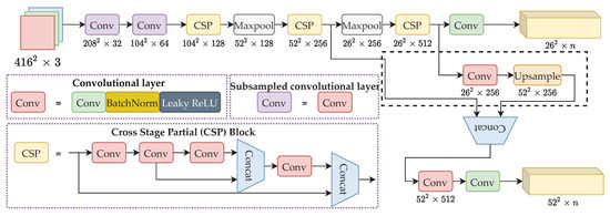
Figure A1.
Naive approach of the YOLO-RTUAV model.
Figure A1.
Naive approach of the YOLO-RTUAV model.
Table A1.
Network architecture of our model and naive approach.
Table A1.
Network architecture of our model and naive approach.
| Naive Solution | Ours | |||||||||||
|---|---|---|---|---|---|---|---|---|---|---|---|---|
| Layer | Type | Filter | Size/Stride | Input Size | Output Size | BFLOPs | Type | Filter | Size/Stride | Input Size | Output Size | BFLOPs |
| 0 | Convolutional | 32 | / 2 | 0.113 | Convolutional | 32 | / 2 | 0.113 | ||||
| 1 | Convolutional | 64 | / 2 | 0.604 | Convolutional | 64 | / 2 | 0.604 | ||||
| 2 | Convolutional | 64 | / 1 | 1.208 | Convolutional | 64 | / 1 | 1.208 | ||||
| 3 | Route 2 | Route 2 | ||||||||||
| 4 | Convolutional | 32 | / 1 | 0.302 | Convolutional | 32 | / 1 | 0.302 | ||||
| 5 | Convolutional | 32 | / 1 | 0.302 | Convolutional | 32 | / 1 | 0.302 | ||||
| 6 | Route 5 4 | Route 5 4 | ||||||||||
| 7 | Convolutional | 64 | / 1 | 0.134 | Convolutional | 64 | / 1 | 0.134 | ||||
| 8 | Route 2 7 | Route 2 7 | ||||||||||
| 9 | Maxpool | / 2 | 0.002 | Maxpool | / 2 | 0.002 | ||||||
| 10 | Convolutional | 128 | / 1 | 1.208 | Convolutional | 128 | / 1 | 1.208 | ||||
| 11 | Route 10 | Route 10 | ||||||||||
| 12 | Convolutional | 64 | / 1 | 0.302 | Convolutional | 64 | / 1 | 0.302 | ||||
| 13 | Convolutional | 64 | / 1 | 0.302 | Convolutional | 64 | / 1 | 0.302 | ||||
| 14 | Route 13 12 | Route 13 12 | ||||||||||
| 15 | Convolutional | 128 | / 1 | 0.134 | Convolutional | 128 | / 1 | 0.134 | ||||
| 16 | Route 10 15 | Route 10 15 | ||||||||||
| 17 | Maxpool | / 2 | 0.001 | Maxpool | / 2 | 0.001 | ||||||
| 18 | Convolutional | 256 | / 1 | 1.208 | Convolutional | 256 | / 1 | 1.208 | ||||
| 19 | Route 18 | Route 18 | ||||||||||
| 20 | Convolutional | 128 | / 1 | 0.302 | Convolutional | 128 | / 1 | 0.302 | ||||
| 21 | Convolutional | 128 | / 1 | 0.302 | Convolutional | 128 | / 1 | 0.302 | ||||
| 22 | Route 21 20 | Route 21 20 | ||||||||||
| 23 | Convolutional | 256 | / 1 | 0.134 | Convolutional | 256 | / 1 | 0.134 | ||||
| 24 | Route 18 23 | Route 18 23 | ||||||||||
| 25 | Convolutional | 27 | / 1 | 0.038 | Convolutional | 36 | / 1 | 0.038 | ||||
| 26 | YOLO | YOLO | ||||||||||
| 27 | Route 25 | Route 25 | ||||||||||
| 28 | Convolutional | 256 | / 1 | 0.019 | Convolutional | 256 | / 1 | 0.019 | ||||
| 29 | Upsample | Upsample | ||||||||||
| 30 | Route 16 | |||||||||||
| 31 | Convolutional | 128 | / 1 | 0.268 | ||||||||
| 32 | Route 29 16 | Route 31 29 | ||||||||||
| 33 | Convolutional | 512 | / 1 | 19.327 | Convolutional | 256 | / 1 | 0.805 | ||||
| 34 | Convolutional | 36 | / 1 | 0.151 | Convolutional | 36 | / 1 | 0.075 | ||||
| 35 | YOLO | YOLO | ||||||||||
To validate if such a modification would impact the detection accuracy, we performed experiments with both the naive and our proposed models. As shown in Table A2, the model size was reduced to around 60%; the FLOPs were reduced to around 70%; the number of parameters were reduced to around 50%. However, a small drop in accuracy was observed. Given the tradeoff between inference time and accuracy, we believe our proposed model struck a balance between them.
Table A2.
COWC dataset.
Table A2.
COWC dataset.
| Model | Input Size | Model Size | BFLOPs | # Param | Precision | Recall | F1 Score | Inference Time (ms) | |||
|---|---|---|---|---|---|---|---|---|---|---|---|
| Tesla T4 | Quadro P5000 | Jetson Nano | |||||||||
| (a) VAID dataset | |||||||||||
| Naive | 14.7MB | 17.23 | 3.68M | 0.8754 | 0.9686 | 0.5770 | 0.7232 | 5.37 | 4.48 | 80.02 | |
| Naive | 14.7MB | 26.09 | 3.68M | 0.9463 | 0.9699 | 0.8795 | 0.9225 | 6.88 | 5.17 | 99.31 | |
| Naive | 14.7MB | 36.80 | 3.68M | 0.9612 | 0.9637 | 0.9465 | 0.9550 | 9.36 | 7.57 | 128.32 | |
| Ours | 5.8MB | 5.13 | 1.44M | 0.8715 | 0.9646 | 0.5686 | 0.7154 | 4.42 | 3.01 | 59.13 | |
| Ours | 5.8MB | 7.77 | 1.44M | 0.9398 | 0.9658 | 0.8714 | 0.9162 | 5.67 | 4.67 | 80.98 | |
| Ours | 5.8MB | 10.95 | 1.44M | 0.9602 | 0.9602 | 0.9433 | 0.9517 | 7.78 | 5.36 | 108.46 | |
| (b) COWC dataset | |||||||||||
| Naive | 14.7 MB | 17.19 | 3.67M | 0.9345 | 0.9001 | 0.9536 | 0.9261 | 5.18 | 14.48 | 79.81 | |
| Naive | 14.7 MB | 26.09 | 3.68M | 0.9405 | 0.8989 | 0.9625 | 0.9296 | 6.59 | 14.05 | 98.21 | |
| Ours | 5.7 MB | 5.10 | 1.43M | 0.9299 | 0.8772 | 0.9422 | 0.9085 | 4.32 | 4.00 | 58.36 | |
| Ours | 5.7 MB | 7.73 | 1.43M | 0.9353 | 0.8853 | 0.9552 | 0.9189 | 5.33 | 13.89 | 78.33 | |
References
- Scherer, J.; Yahyanejad, S.; Hayat, S.; Yanmaz, E.; Andre, T.; Khan, A.; Vukadinovic, V.; Bettstetter, C.; Hellwagner, H.; Rinner, B. An autonomous multi-UAV system for search and rescue. In Proceedings of the First Workshop on Micro Aerial Vehicle Networks, Systems, and Applications for Civilian Use, Florence, Italy, 19–22 May 2015; pp. 33–38. [Google Scholar]
- Alotaibi, E.T.; Alqefari, S.S.; Koubaa, A. Lsar: Multi-uav collaboration for search and rescue missions. IEEE Access 2019, 7, 55817–55832. [Google Scholar] [CrossRef]
- Messina, G.; Modica, G. Applications of UAV thermal imagery in precision agriculture: State of the art and future research outlook. Remote Sens. 2020, 12, 1491. [Google Scholar] [CrossRef]
- Liu, S.; Wang, S.; Shi, W.; Liu, H.; Li, Z.; Mao, T. Vehicle tracking by detection in UAV aerial video. Sci. China Inf. Sci. 2019, 62, 24101. [Google Scholar] [CrossRef] [Green Version]
- Song, W.; Li, S.; Guo, Y.; Li, S.; Hao, A.; Qin, H.; Zhao, Q. Meta transfer learning for adaptive vehicle tracking in UAV videos. In Proceedings of the International Conference on Multimedia Modeling, Daejeon, Korea, 5–8 January 2020; pp. 764–777. [Google Scholar]
- Zhao, X.; Pu, F.; Wang, Z.; Chen, H.; Xu, Z. Detection, tracking, and geolocation of moving vehicle from uav using monocular camera. IEEE Access 2019, 7, 101160–101170. [Google Scholar] [CrossRef]
- Green, D.R.; Hagon, J.J.; Gómez, C.; Gregory, B.J. Using low-cost UAVs for environmental monitoring, mapping, and modelling: Examples from the coastal zone. In Coastal Management; Elsevier: Amsterdam, The Netherlands, 2019; pp. 465–501. [Google Scholar]
- Tripolitsiotis, A.; Prokas, N.; Kyritsis, S.; Dollas, A.; Papaefstathiou, I.; Partsinevelos, P. Dronesourcing: A modular, expandable multi-sensor UAV platform for combined, real-time environmental monitoring. Int. J. Remote Sens. 2017, 38, 2757–2770. [Google Scholar] [CrossRef]
- Girshick, R.; Donahue, J.; Darrell, T.; Malik, J. Rich feature hierarchies for accurate object detection and semantic segmentation. In Proceedings of the IEEE Conference on Computer Vision and Pattern Recognition, Columbus, OH, USA, 23–28 June 2014; pp. 580–587. [Google Scholar]
- Girshick, R. Fast r-cnn. In Proceedings of the IEEE International Conference on Computer Vision, Santiago, Chile, 7–13 December 2015; pp. 1440–1448. [Google Scholar]
- Ren, S.; He, K.; Girshick, R.; Sun, J. Faster r-cnn: Towards real-time object detection with region proposal networks. arXiv 2015, arXiv:1506.01497. [Google Scholar] [CrossRef] [PubMed] [Green Version]
- Redmon, J.; Divvala, S.; Girshick, R.; Farhadi, A. You only look once: Unified, real-time object detection. In Proceedings of the IEEE Conference on Computer Vision and Pattern Recognition, Las Vegas, NV, USA, 27–30 June 2016; pp. 779–788. [Google Scholar]
- Redmon, J.; Farhadi, A. YOLO9000: Better, faster, stronger. In Proceedings of the IEEE Conference on Computer Vision and Pattern Recognition, Honolulu, HI, USA, 21–26 July 2017; pp. 7263–7271. [Google Scholar]
- Redmon, J.; Farhadi, A. Yolov3: An incremental improvement. arXiv 2018, arXiv:1804.02767. [Google Scholar]
- Bochkovskiy, A.; Wang, C.Y.; Liao, H.Y.M. Yolov4: Optimal speed and accuracy of object detection. arXiv 2020, arXiv:2004.10934. [Google Scholar]
- Liu, W.; Anguelov, D.; Erhan, D.; Szegedy, C.; Reed, S.; Fu, C.Y.; Berg, A.C. Ssd: Single shot multibox detector. In Proceedings of the European Conference on Computer Vision, Amsterdam, The Netherlands, 11–14 October 2016; pp. 21–37. [Google Scholar]
- Fu, C.Y.; Liu, W.; Ranga, A.; Tyagi, A.; Berg, A.C. Dssd: Deconvolutional single shot detector. arXiv 2017, arXiv:1701.06659. [Google Scholar]
- Lin, T.Y.; Maire, M.; Belongie, S.J.; Hays, J.; Perona, P.; Ramanan, D.; Dollár, P.; Zitnick, C.L. Microsoft COCO: Common Objects in Context. In Proceedings of the European Conference on Computer Vision, Zurich, Switzerland, 6–12 September 2014; pp. 740–755. [Google Scholar]
- Everingham, M.; Gool, L.; Williams, C.K.; Winn, J.; Zisserman, A. The Pascal Visual Object Classes (VOC) Challenge. Int. J. Comput. Vis. 2010, 88, 303–338. [Google Scholar] [CrossRef] [Green Version]
- Liu, Y.; Yang, F.; Hu, P. Small-object detection in UAV-captured images via multi-branch parallel feature pyramid networks. IEEE Access 2020, 8, 145740–145750. [Google Scholar] [CrossRef]
- Liu, M.; Wang, X.; Zhou, A.; Fu, X.; Ma, Y.; Piao, C. UAV-YOLO: Small Object Detection on Unmanned Aerial Vehicle Perspective. Sensors 2020, 20, 2238. [Google Scholar] [CrossRef] [PubMed] [Green Version]
- Pham, M.T.; Courtrai, L.; Friguet, C.; Lefèvre, S.; Baussard, A. YOLO-Fine: One-stage detector of small objects under various backgrounds in remote sensing images. Remote Sens. 2020, 12, 2501. [Google Scholar] [CrossRef]
- Lin, H.Y.; Tu, K.C.; Li, C.Y. VAID: An Aerial Image Dataset for Vehicle Detection and Classification. IEEE Access 2020, 8, 212209–212219. [Google Scholar] [CrossRef]
- Mundhenk, T.N.; Konjevod, G.; Sakla, W.A.; Boakye, K. A large contextual dataset for classification, detection and counting of cars with deep learning. In Proceedings of the European Conference on Computer Vision, Amsterdam, The Netherlands, 11–14 October 2016; pp. 785–800. [Google Scholar]
- Ma, B.; Liu, Z.; Jiang, F.; Yan, Y.; Yuan, J.; Bu, S. Vehicle Detection in Aerial Images Using Rotation-Invariant Cascaded Forest. IEEE Access 2019, 7, 59613–59623. [Google Scholar] [CrossRef]
- Raj, S.U.; Manikanta, M.V.; Harsitha, P.S.S.; Leo, M.J. Vacant Parking Lot Detection System Using Random Forest Classification. In Proceedings of the 3rd International Conference on Computing Methodologies and Communication (ICCMC), Erode, India, 27–29 March 2019; Volume 2019, pp. 454–458. [Google Scholar]
- Zhou, H.; Wei, L.; Lim, C.P.; Creighton, D.; Nahavandi, S. Robust Vehicle Detection in Aerial Images Using Bag-of-Words and Orientation Aware Scanning. IEEE Trans. Geosci. Remote Sens. 2018, 56, 7074–7085. [Google Scholar] [CrossRef]
- Liu, K.; Mattyus, G. Fast Multiclass Vehicle Detection on Aerial Images. IEEE Geosci. Remote Sens. Lett. 2015, 12, 1938–1942. [Google Scholar]
- Gleason, J.; Nefian, A.V.; Bouyssounousse, X.; Fong, T.; Bebis, G. Vehicle detection from aerial imagery. In Proceedings of the 2011 IEEE International Conference on Robotics and Automation, Shanghai, China, 9–13 May 2011; pp. 2065–2070. [Google Scholar]
- Xu, Y.; Yu, G.; Wu, X.; Wang, Y.; Ma, Y. An Enhanced Viola-Jones Vehicle Detection Method From Unmanned Aerial Vehicles Imagery. IEEE Trans. Intell. Transp. Syst. 2017, 18, 1845–1856. [Google Scholar] [CrossRef]
- Chen, Z.; Wang, C.; Wen, C.; Teng, X.; Chen, Y.; Guan, H.; Luo, H.; Cao, L.; Li, J. Vehicle Detection in High-Resolution Aerial Images via Sparse Representation and Superpixels. IEEE Trans. Geosci. Remote. Sens. 2016, 54, 103–116. [Google Scholar] [CrossRef]
- Cao, S.; Yu, Y.; Guan, H.; Peng, D.; Yan, W. Affine-Function Transformation-Based Object Matching for Vehicle Detection from Unmanned Aerial Vehicle Imagery. Remote Sens. 2019, 11, 1708. [Google Scholar] [CrossRef] [Green Version]
- Cao, L.; Luo, F.; Chen, L.; Sheng, Y.; Wang, H.; Wang, C.; Ji, R. Weakly supervised vehicle detection in satellite images via multi-instance discriminative learning. Pattern Recognit. 2017, 64, 417–424. [Google Scholar] [CrossRef]
- Tong, K.; Wu, Y.; Zhou, F. Recent advances in small object detection based on deep learning: A review. Image Vis. Comput. 2020, 97, 103910. [Google Scholar] [CrossRef]
- Srivastava, S.; Narayan, S.; Mittal, S. A survey of deep learning techniques for vehicle detection from UAV images. J. Syst. Archit. 2021, 117, 102152. [Google Scholar] [CrossRef]
- Eggert, C.; Brehm, S.; Winschel, A.; Zecha, D.; Lienhart, R. A closer look: Small object detection in faster R-CNN. In Proceedings of the 2017 IEEE International Conference on Multimedia and Expo (ICME), Hong Kong, China, 10–14 July 2017; Volume 2017, pp. 421–426. [Google Scholar]
- Cao, C.; Wang, B.; Zhang, W.; Zeng, X.; Yan, X.; Feng, Z.; Liu, Y.; Wu, Z. An Improved Faster R-CNN for Small Object Detection. IEEE Access 2019, 7, 106838–106846. [Google Scholar] [CrossRef]
- Ren, Y.; Zhu, C.; Xiao, S. Small Object Detection in Optical Remote Sensing Images via Modified Faster R-CNN. Appl. Sci. 2018, 8, 813. [Google Scholar] [CrossRef] [Green Version]
- Guan, L.; Wu, Y.; Zhao, J. SCAN: Semantic Context Aware Network for Accurate Small Object Detection. Int. J. Comput. Intell. Syst. 2018, 11, 936–950. [Google Scholar] [CrossRef] [Green Version]
- Cao, G.; Xie, X.; Yang, W.; Liao, Q.; Shi, G.; Wu, J. Feature-fused SSD: Fast detection for small objects. In Proceedings of the Ninth International Conference on Graphic and Image Processing (ICGIP 2017), Qingdao, China, 14–16 October 2017; Volume 10615. [Google Scholar]
- Cui, L.; Ma, R.; Lv, P.; Jiang, X.; Gao, Z.; Zhou, B.; Xu, M. MDSSD: Multi-scale deconvolutional single shot detector for small objects. Sci. China Ser. Inf. Sci. 2020, 63, 120113. [Google Scholar] [CrossRef] [Green Version]
- Zhang, S.; Wen, L.; Bian, X.; Lei, Z.; Li, S.Z. Single-Shot Refinement Neural Network for Object Detection. In Proceedings of the 2018 IEEE/CVF Conference on Computer Vision and Pattern Recognition, Salt Lake City, UT, USA, 18–23 June 2018; pp. 4203–4212. [Google Scholar]
- Yang, M.Y.; Liao, W.; Li, X.; Rosenhahn, B. Deep Learning for Vehicle Detection in Aerial Images. In Proceedings of the 2018 25th IEEE International Conference on Image Processing (ICIP), Athens, Greece, 7–10 October 2018; pp. 3079–3083. [Google Scholar]
- Sommer, L.; Schumann, A.; Schuchert, T.; Beyerer, J. Multi Feature Deconvolutional Faster R-CNN for Precise Vehicle Detection in Aerial Imagery. In Proceedings of the 2018 IEEE Winter Conference on Applications of Computer Vision (WACV), Lake Tahoe, NV, USA, 12–15 March 2018; pp. 635–642. [Google Scholar]
- Zhong, J.; Lei, T.; Yao, G. Robust Vehicle Detection in Aerial Images Based on Cascaded Convolutional Neural Networks. Sensors 2017, 17, 2720. [Google Scholar] [CrossRef] [Green Version]
- Rajput, P.; Nag, S.; Mittal, S. Detecting Usage of Mobile Phones using Deep Learning Technique. In Proceedings of the 6th EAI International Conference on Smart Objects and Technologies for Social Good, Antwerp, Belgium, 14–16 September 2020; pp. 96–101. [Google Scholar]
- Tang, T.; Deng, Z.; Zhou, S.; Lei, L.; Zou, H. Fast vehicle detection in UAV images. In Proceedings of the 2017 International Workshop on Remote Sensing with Intelligent Processing (RSIP), Shanghai, China, 19–21 May 2017; pp. 1–5. [Google Scholar]
- Sommer, L.; Nie, K.; Schumann, A.; Schuchert, T.; Beyerer, J. Semantic labeling for improved vehicle detection in aerial imagery. In Proceedings of the 2017 14th IEEE International Conference on Advanced Video and Signal Based Surveillance (AVSS), Lecce, Italy, 29 August–1 September 2017; pp. 1–6. [Google Scholar]
- Xie, X.; Yang, W.; Cao, G.; Yang, J.; Zhao, Z.; Chen, S.; Liao, Q.; Shi, G. Real-Time Vehicle Detection from UAV Imagery. In Proceedings of the 2018 IEEE Fourth International Conference on Multimedia Big Data (BigMM), Xi’an, China, 13–16 September 2018; pp. 1–5. [Google Scholar]
- Yang, J.; Xie, X.; Yang, W. Effective Contexts for UAV Vehicle Detection. IEEE Access 2019, 7, 85042–85054. [Google Scholar] [CrossRef]
- Carlet, J.; Abayowa, B. Fast Vehicle Detection in Aerial Imagery. arXiv 2017, arXiv:1709.08666. [Google Scholar]
- Ammour, N.; Alhichri, H.S.; Bazi, Y.; Benjdira, B.; Alajlan, N.; Zuair, M.A.A. Deep Learning Approach for Car Detection in UAV Imagery. Remote Sens. 2017, 9, 312. [Google Scholar] [CrossRef] [Green Version]
- Audebert, N.; Saux, B.L.; Lefèvre, S. Segment-before-detect: Vehicle detection and classification through semantic segmentation of aerial images. Remote Sens. 2017, 9, 368. [Google Scholar] [CrossRef] [Green Version]
- Huang, R.; Pedoeem, J.; Chen, C. YOLO-LITE: A Real-Time Object Detection Algorithm Optimized for Non-GPU Computers. In Proceedings of the 2018 IEEE International Conference on Big Data (Big Data), Seattle, WA, USA, 10–13 December 2018; pp. 2503–2510. [Google Scholar]
- Zhang, P.; Zhong, Y.; Li, X. SlimYOLOv3: Narrower, Faster and Better for Real-Time UAV Applications. In Proceedings of the 2019 IEEE/CVF International Conference on Computer Vision Workshop (ICCVW), Seoul, Korea, 27–28 October 2019. [Google Scholar]
- Kim, S.J.; Park, S.; Na, B.; Yoon, S. Spiking-YOLO: Spiking Neural Network for Energy-Efficient Object Detection. In Proceedings of the AAAI Conference on Artificial Intelligence, Hilton New York Midtown, NY, USA, 7–12 February 2020; Volume 34, pp. 11270–11277. [Google Scholar]
- Wong, A.; Famouri, M.; Shafiee, M.J.; Li, F.; Chwyl, B.; Chung, J. YOLO Nano: A Highly Compact You Only Look Once Convolutional Neural Network for Object Detection. arXiv 2019, arXiv:1910.01271. [Google Scholar]
- Ringwald, T.; Sommer, L.; Schumann, A.; Beyerer, J.; Stiefelhagen, R. UAV-Net: A Fast Aerial Vehicle Detector for Mobile Platforms. In Proceedings of the 2019 IEEE/CVF Conference on Computer Vision and Pattern Recognition Workshops (CVPRW), Long Beach, CA, USA, 16–17 June 2019; pp. 544–552. [Google Scholar]
- He, Y.; Pan, Z.; Li, L.; Shan, Y.; Cao, D.; Chen, L. Real-Time Vehicle Detection from Short-range Aerial Image with Compressed MobileNet. In Proceedings of the 2019 International Conference on Robotics and Automation (ICRA), Montreal, Canada, 20–24 May 2019; pp. 8339–8345. [Google Scholar]
- Mandal, M.; Shah, M.; Meena, P.; Devi, S.; Vipparthi, S.K. AVDNet: A Small-Sized Vehicle Detection Network for Aerial Visual Data. IEEE Geosci. Remote Sens. Lett. 2020, 17, 494–498. [Google Scholar] [CrossRef] [Green Version]
- Azimi, S.M. ShuffleDet: Real-Time Vehicle Detection Network in On-Board Embedded UAV Imagery. In Proceedings of the European Conference on Computer Vision (ECCV) Workshops, Munich, Germany, 8–14 September 2018; pp. 88–99. [Google Scholar]
- Lin, T.Y.; Dollár, P.; Girshick, R.; He, K.; Hariharan, B.; Belongie, S. Feature pyramid networks for object detection. In Proceedings of the IEEE Conference on Computer Vision and Pattern Recognition, Honolulu, HI, USA, 21–26 July 2017; pp. 2117–2125. [Google Scholar]
- Misra, D. Mish: A self regularized non-monotonic neural activation function. arXiv 2019, arXiv:1908.08681. [Google Scholar]
- Zheng, Z.; Wang, P.; Liu, W.; Li, J.; Ye, R.; Ren, D. Distance-IoU loss: Faster and better learning for bounding box regression. In Proceedings of the AAAI Conference on Artificial Intelligence, Hilton New York Midtown, NY, USA, 7–12 February 2020; Volume 34, pp. 12993–13000. [Google Scholar]
- Wu, Y.; Kirillov, A.; Massa, F.; Lo, W.Y.; Girshick, R. Detectron2. 2019. Available online: https://github.com/facebookresearch/detectron2 (accessed on 8 August 2021).
- Ge, Z.; Liu, S.; Wang, F.; Li, Z.; Sun, J. YOLOX: Exceeding YOLO Series in 2021. arXiv 2021, arXiv:2107.08430. [Google Scholar]


Publisher’s Note: MDPI stays neutral with regard to jurisdictional claims in published maps and institutional affiliations. |
© 2021 by the authors. Licensee MDPI, Basel, Switzerland. This article is an open access article distributed under the terms and conditions of the Creative Commons Attribution (CC BY) license (https://creativecommons.org/licenses/by/4.0/).