Article

Spatiotemporal Analysis of Sea Ice Leads in the Arctic Ocean Retrieved from IceBridge Laxon Line Data 2012–2018

1
NSF Spatiotemporal Innovation Center, Department of Geography and Geoinformation Science, George Mason University, Fairfax, VA 22030, USA
2
Center for Advanced Measurements in Extreme Environments, Department of Earth and Planetary Sciences, University of Texas at San Antonio, San Antonio, TX 78249, USA
3
Department of Geography, Geology and Planning, Missouri State University, Springfield, MO 65897, USA
*
Author to whom correspondence should be addressed.
Remote Sens. 2021, 13(20), 4177; https://doi.org/10.3390/rs13204177
Submission received: 7 August 2021 / Revised: 6 October 2021 / Accepted: 13 October 2021 / Published: 19 October 2021
(This article belongs to the Topic Climate Change and Environmental Sustainability)

Abstract

:
The ocean and atmosphere exert stresses on sea ice that create elongated cracks and leads which dominate the vertical exchange of energy, especially in cold seasons, despite covering only a small fraction of the surface. Motivated by the need of a spatiotemporal analysis of sea ice lead distribution, a practical workflow was developed to classify the high spatial resolution aerial images DMS (Digital Mapping System) along the Laxon Line in the NASA IceBridge Mission. Four sea ice types (thick ice, thin ice, open water, and shadow) were identified, and relevant sea ice lead parameters were derived for the period of 2012–2018. The spatiotemporal variations of lead fraction along the Laxon Line were verified by ATM (Airborne Topographic Mapper) surface height data and correlated with coarse spatial resolution sea ice motion, air temperature, and wind data through multiple regression models. We found that the freeboard data derived from sea ice leads were compatible with other products. The temperature and ice motion vorticity were the leading factors of the formation of sea ice leads, followed by wind vorticity and kinetic moments of ice motion.

1. Introduction

Arctic sea ice functions as a sensitive indicator of global warming because sea ice responds to even a small increase in temperature [1,2,3]. On the other hand, Arctic sea ice is also an important driver of climate change, and it plays an important role in the Earth’s solar radiation budget. This is due to how sea ice has a significantly higher albedo compared to that of the water surface. Therefore, when the Arctic sea ice starts to melt, the oceans absorb more solar radiation and warm up, accelerating the melting of sea ice in a positive feedback [4].
Among all types of sea ice features, leads have unique characteristics. A lead is an elongated crack in the sea ice developed by the divergence or shear of floating ice floes when moving with currents and winds [5]. Leads vary in width from meters to hundreds of meters depending on their development and the directions of surrounding pressure and tension. Since a lead is physically an open water body, thin ice, or mixed open water and thin ice within (thicker) sea ice floe or between sea ice floes, it allows the direct interaction between the atmosphere and the ocean and is the only (or major) channel in the cold Arctic. Thus, leads play an important role in the local radiation energy budget, ship navigation, and the Arctic sea ice ecosystem [6]. In particular, they dominate the vertical exchange of energy during winter when turbulent heat fluxes over leads can be orders of magnitude larger than that over thick ice. The width of leads and their orientation markedly influence associated vertical sensible and latent heat fluxes and associated cloud formation [7,8]. Recent studies suggest that these fluxes could influence the atmospheric properties tens to hundreds of kilometers downstream [9,10,11]. Even a small fraction of thin ice and open water within the sea ice pack can significantly modify the total energy transfer between the ocean and the atmosphere [12]. Furthermore, leads are elusive and inconsistent features. If sea water temperature drops below around −1.8 °C, the open water within a lead quickly refreezes (in a few hours), and leads will be partly or entirely covered by a thin layer of new ice [13,14,15]. Therefore, leads are an important component of the Arctic surface energy budget, and more quantitative studies are needed to explore and model their impact on the Arctic climate system.
Arctic climate models require a detailed spatial distribution of leads to simulate interactions between the ocean and the atmosphere. Remote sensing techniques can be used to extract sea ice physical features and parameters and calibrate or validate climate models [16]. However, most of the sea ice leads studies focus on low-moderate resolution (~1 km) imagery such as Moderate Resolution Imaging Spectroradiometer (MODIS) or Advanced Very High-Resolution Radiometer (AVHRR) [17,18,19,20], which cannot detect small leads, such as those smaller than 100 m. On the other hand, high spatial resolution (HSR) images such as aerial photos are discrete and heterogeneous in space and time, i.e., images usually cover only a small and discontinuous area with time intervals between images varying from a few seconds to several months [21,22]. Therefore, it is difficult to weave these small pieces into a coherent large-scale picture, which is important for coupled sea ice and climate modeling and verification. Onana et al. used operational IceBridge airborne visible DMS (Digital Mapping System) imagery and laser altimetry measurements to detect sea ice leads and classify open water, thin ice (new ice, grease ice, frazil ice, and nilas), and gray ice [23]. Miao et al. utilized an object-based image classification scheme to classify water, ice/snow, melt ponds, and shadow [24]. However, the workflow used in Miao et al. was based on some independent proprietary software, which is not suitable for batch processing in an operational environment. In contrast, Wright and Polashenski developed an Open Source Sea Ice Processing (OSSP) package for detecting sea ice surface features in high-resolution optical imagery [25,26]. Based on the OSSP package, Wright et al. investigated the behavior of meltwater on first-year and multiyear ice during summer melting seasons [26]. Following this approach, Sha et al. further improved and integrated the OSSP modules into an on-demand service in cloud computing-based infrastructure for operational usage [22].
Following the previous studies, this paper focuses on the spatiotemporal analysis of sea ice lead distribution through NASA’s Operation IceBridge images, which used a systematic sampling scheme to collect high spatial resolution DMS aerial photos along critical flight lines in the Arctic. A practical workflow was developed to classify the DMS images along the Laxon Line into four classes, i.e., thick ice, thin ice, water, and shadow, and to extract sea ice lead and thin ice during the missions 2012–2018. Finally, the spatiotemporal variations of lead fraction along the Laxon Line were verified by ATM surface height data (freeboard), and correlated with sea ice motion, air temperature, and wind data. The paper is organized as follows: Section 2 provides a background description of DMS imagery, the Laxon Line collection, and auxiliary sea ice data. Section 3 describes the methodology and workflow. Section 4 presents and discusses the spatiotemporal variations of leads. The summary and conclusions are provided in Section 5.

2. Dataset

2.1. IceBridge DMS Images and Study Area

This study uses IceBridge DMS images to detect Arctic sea ice leads along the Laxon Line one day over the course of 7 years in 2012–2018, since these are the longest continuous yearly data available in this Arctic region. The DMS images were collected during the IceBridge sea ice flights using an airborne digital camera. DMS has a high spatial resolution 0.1–2.5 m [27], depending on the aircraft flight height. It has three natural color (red, green, and blue) bands, and each image has a field of view of approximately 400 m by 600 m. The IceBridge campaigns had been designed to survey the Arctic region in March and April since 2009 to partially fill the temporal gap between the ICESat (2003–2009) and ICESat-2 (2018–present) missions.
DMS images are collected, processed, and maintained by the Airborne Sensor Facility located at the NASA AMES Research Center. We downloaded the Level 1B geolocated and orthorectified images for the Arctic Laxon Line in spring from 2012 to 2018 from the NASA National Snow and Ice Data Center Distributed Active Archive Center (NSIDC DAAC) (https://nsidc.org/data/iodms1b) (accessed on 6 August 2021). The Laxon Line starts from the Thule Air Base, Greenland to Fairbanks, AK, USA, transiting across the Arctic Ocean (Figure 1). It passes through both multiyear ice (MYI) regions in the north of the Canadian Archipelago and the first-year ice (FYI) regions in northern Alaska. Thus, sea ice data along this line provides useful insights on the transition of sea ice conditions over the Central Arctic in the spring. Furthermore, the IceBridge mission collected data along this track repeatedly every year from 2012 to 2018, which is appropriate for spatiotemporal analysis of sea ice leads. The overall DMS image collection along the Laxon Line is 106,674 aerial photos (1.54 TB) with an overlap of 60–90% along the track. The photo distribution from 2012–2018 is summarized in Table 1. The overall distance of the Laxon Line is around 3398 km, and the distance for the overlapped track through the years is around 2437 km.

2.2. Auxiliary Sea Ice Data

2.2.1. AMSR Data

AMSR (Advanced Microwave Scanning Radiometer) is a passive microwave satellite sensor developed by the Japan Aerospace Exploration Agency. Due to its low spatial resolution, the AMSR data can only be used to examine sea ice concentrations at the regional scale. We collected the AMSR-E/AMSR-2 Unified Level 3 daily brightness temperature and sea ice concentration data which has a spatial resolution of 25 km through NSIDC (Table 2) [28]. The data contain vertically polarized and horizontally polarized brightness temperatures at four frequency channels: 18.7, 23.8, 36.5, and 89.0 GHz. The Arctic sea ice concentration (SIC) was calculated by the NASA Team 2 (NT2) algorithm, which provides <2% of error compared with the high-resolution optical data [29,30,31]. The collected AMSR data coincides with the days of the IceBridge mission from 2012 to 2018, so that the SIC can be compared with that retrieved from the DMS images. Furthermore, the passive microwave data can be used to calculate thin ice concentration (TIC). Röhrs and Kaleschke used brightness temperatures at the vertically polarized 18.7 and 89.0 GHz to identify water and thin ice (i.e., new ice, nilas, and pancake ice) from thick ice, and the sea ice leads and TIC showed a good agreement with the MODIS, Envisat ASAR, and CryoSat-2 data [14]. In this study, we calculated TIC following the Röhrs and Kaleschke’s algorithm. The coarser spatial resolution of 25 km of TIC were compared with our lead and thin ice fractions retrieved from the DMS images.

2.2.2. ATM Surface Height Data (DMS Level)

Our DMS-based lead detection results can be used to cross-validate sea ice freeboard products derived from IceBridge Airborne Topographic Mapper (ATM) Level 1B data [23]. The ATM is an airborne conically scanning laser altimeter with a wavelength of 532 nm. A laser pulse is emitted from the ATM at a rate of 5 kHz, and it has ~1 m of footprint at a typical 500 m altitude above the surface. Since ATM covers exactly the same location and time with the DMS images with a smaller cross-track width (~400 m), DMS images are usually used as good reference for extracting the ATM-based freeboard data [32,33]. In this study, the ATM data are resampled in a 2 m grid and projected to the same projection system as DMS (NSIDC sea ice polar stereographic North) to match the geographical location. After retrieving thin ice and leads through DMS images, we geographically linked the leads with the ATM data to extract freeboard variations along the Laxon Line, and compare with freeboard data derived from SILDAMS (Sea Ice Lead Detection Algorithm) [23,32].

2.3. Oceanic and Atmospheric Geophysical Parameters

NSIDC provides sea ice motion data (nsidc.org/data/NSIDC-0116) with a spatial resolution of 25 km on the Equal-Area Scalable Earth grid [34]. This sea ice motion vector is derived from multiple data sources, including AVHRR, AMSR-E, SMMR, SSMI, SSMI/S satellite sensors, International Arctic Buoy Program (IABP) buoys, and the National Center for Environmental Prediction/National Center for Atmospheric Research (NCEP/NCAR) reanalysis.
We also acquired a global sea ice type product provided by the European Organization for the Exploitation of Meteorological Satellites (EUMETSAT) Ocean and Sea Ice Satellite Application Facility (OSI SAF, www.osi-saf.org) (6 August 2021) [35]. This product assigns different sea ice types, such as multiyear ice (MYI), first-year ice (FYI), and open water, from various satellite data. This is a daily product and has 10 km of spatial resolution.
Other data we used included air temperature (2 m above sea level) and wind velocity data coincident with the DMS images acquired from the European Centre for Medium-Range Weather Forecasts ERA-5 reanalysis. The ERA-5 product has 0.25° spatial resolution and consists of hourly variables, and we integrated this hourly data into daily products and resampled them to 25 km resolution to match the ice motion data. This ERA-5 product was downloaded from the Climate Data Store (cds.climate.copernicus.eu) of the Copernicus Climate Change Service.
In this study, the high spatial resolution lead fractions derived from DMS along the Laxon Line were linearly regressed with the coarse spatial resolution sea ice motion, air temperature, and wind velocity products to identify potential significant drivers.

3. Methods

3.1. Batch Classification Processing Workflow

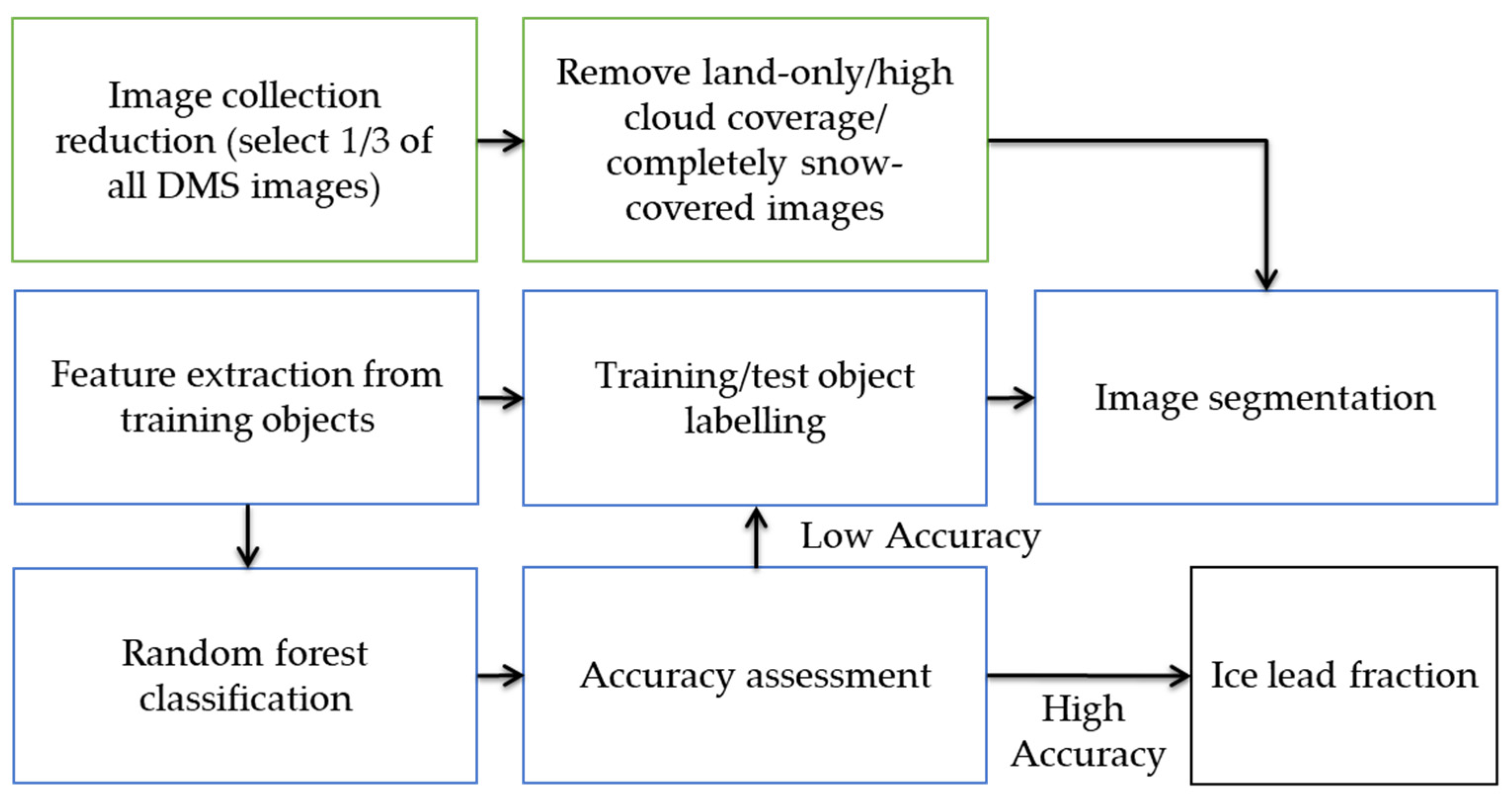
Since the IceBridge DMS images are highly overlapped along the track (60–90%), we selected one image from every three consecutive images along the Laxon Line to reduce the computation burden. All images in continental land masses and poor-quality images due to overwhelming cloud coverage and low lighting conditions were manually removed, finally generating a collection of sea ice lead images (Figure 2).
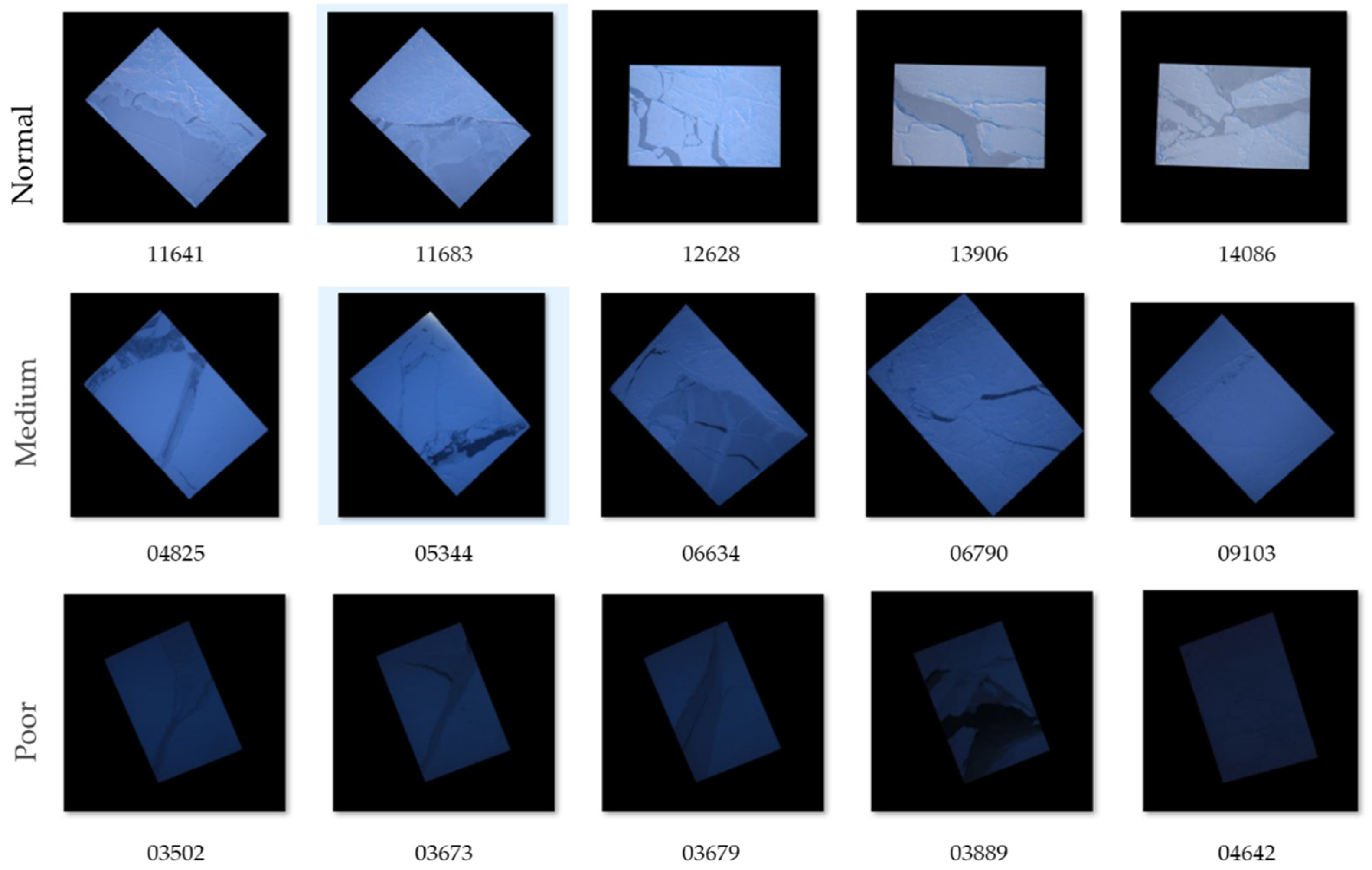
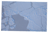
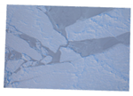
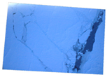
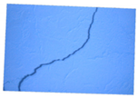
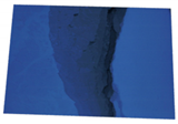
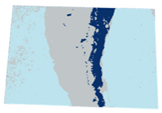
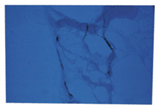
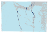
The object-based classification scheme was designed based on the color and texture of sea ice features on DMS images. Four sea ice classes were defined: (1) thick ice is usually thick ice or snow-covered ice with a high albedo; (2) thin ice is usually fresh and newly formed ice, which has a smooth surface with a low albedo, since solar radiation is partially absorbed by the water beneath it; (3) open water is dark and smooth due to its strong absorbance of solar radiation; and (4) shadow is within a thick-ice area and is a relative dark feature projecting on the ice surface by surrounding ridges or snow dunes. DMS images collected in different years have different lighting conditions, which affects the image quality (Table 1). Furthermore, even in the same year, the quality of images was quite distinctive due to the local cloud coverage and lighting conditions, as shown in Figure 3. For example, three subgroups were identified in 2012 DMS images: normal images contained regular sea ice scenes with an appropriate exposure and contrast, and all sea ice classes were recognizable by color and texture; gray images were partially cloudy images with a poor lighting condition, so they were relatively dark, and shadows were difficult to detect; and poor images were under extremely poor lighting conditions, and the boundaries between water, thick ice, and thin ice were blurred due to low contrast.
Therefore, training samples were selected using a divide-and-conquer strategy based on image quality. All DMS images taken in 2013, 2015, 2016, and 2018 were under good lighting conditions, and training samples were selected for all four sea ice features. However, the images taken for the other three years were processed in different ways. The training samples for all images taken in 2012, 2014, and 2017 were only selected for thin ice, open water, and thick ice, without considering shadow due to low lighting conditions. Furthermore, the 2012 images were manually classified into three subgroups, i.e., normal, medium, and poor. The 2014 images were manually classified into two subgroups, i.e., normal and medium, and all poor images were abandoned due to serious vignetting, caused by light hitting the lens aperture at a large angle, and significantly reduced brightness values on the four corners of the image. The 2017 images were all classified into the medium subgroup only. In summary, the independent training samples were collected for each subgroup and year for supervised classification.
The OSSP package uses an object-based classification scheme. For each image, the watershed segmentation method is used to convert pixels into objects. Therefore, training samples are labelled at the object level. Only distinctive and typical sea ice objects are selected across the whole scene, and each sea ice class has around 120–250 objects. The attributes of objects such as color values, band ratios, textures, and shape indexes are calculated and served as supervised classification features. Based on these training datasets, the OSSP package uses the random forest classification method to label all unknown objects in DMS images [24,25].
To evaluate the accuracy of classification results, the independent test object samples were also collected. Table 3 lists the selected image and object numbers for the training and testing process of each classification group. Finally, the confusion matrix was generated at the pixel level and was used for calculating the overall accuracy, user’s accuracy, producer’s accuracy, and Kappa coefficient.

3.2. Sea Ice Leads Parameters Definitions

Based on the classified result in each surface type, we derived the sea ice leads by combining thin ice and open water. Then, the sea ice lead fraction, open water fraction, thin ice fraction, and sea ice concentration were calculated on a per-scene basis. The sea ice lead fraction for each DMS image can be calculated using the following equations:
Sea Ice Lead Fraction (SILF):
SILF = (ThinIce + OpenWater)/(ThickIce + ThinIce + OpenWater + Shadow) ∗ 100,
where ThinIce, OpenWater, ThickIce, and Shadow are pixel numbers of classified thin ice area, open water, thick ice, and shadow for a DMS image, respectively.

3.3. Spatiotemporal Analysis with Auxiliary Sea Ice Data

The auxiliary sea ice datasets can be used to assess the DMS-based lead detection results to deepen the understanding of the formation mechanism of leads. In this research, first, our lead detection result was used to determine local sea reference height and calculate the sea ice freeboard. This retrieved freeboard was compared with the existing NSIDC freeboard data at the scale of 400 m [36]. Furthermore, the coincident AMSR thin ice concentration (TIC) data, and the geophysical atmosphere and ocean data, such as air temperature, wind velocity, and sea ice motion, were compared with the lead fraction results.
Based on our DMS lead detection algorithm, sea ice freeboards were retrieved from the ATM lidar data using the same method as in [32]. Specifically, we removed variations in the instantaneous sea surface height by subtracting geoid and ocean tide height. Then, we calculated the freeboard by subtracting locally determined leads surface height (zshh) from the corrected height (Hcorr).
Freeboard = Hcorr − zshh,
where zshh is determined from the sets of individual lead elevation estimates through ordinary kriging. We calculated the mean freeboard for each DMS image (around 400 m by 600 m) and resampled the value to 400 m resolution. On the other hand, Kurtz et al. used an automated lead detection algorithm through the minimal signal transform [23,32] and then retrieved the freeboard at the resolution of 400 m. Therefore, the two products can be compared and cross-verified at this scale.
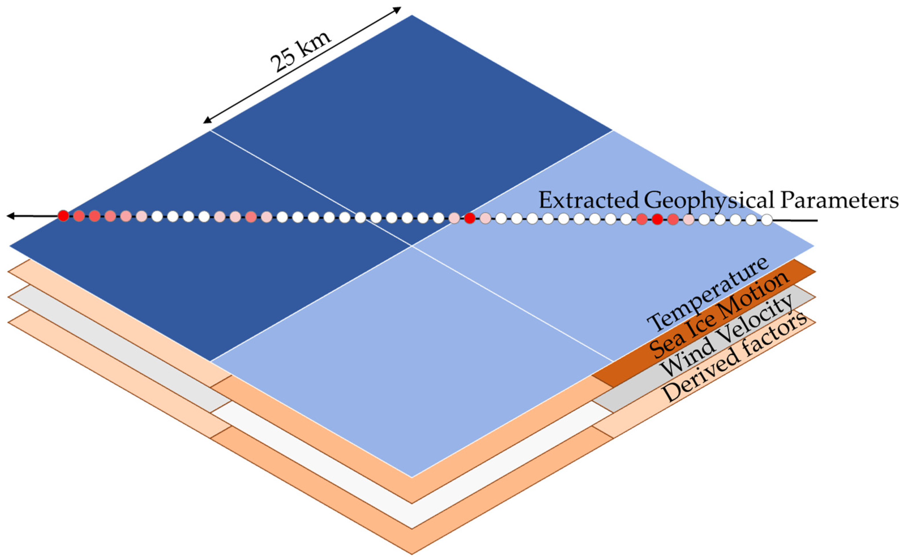
TIC could be calculated from the AMSR as described in Röhrs and Kaleschke [14] with a rather coarse spatial resolution of 25 km. This AMSR-based TIC represents the existence of open water and thin ice on sea ice leads. This TIC is conceptually equivalent to our SILF. Since the AMSR and DMS have different resolutions and geographical coverage, they cannot be compared directly. Therefore, we resampled and averaged the DMS-based ice lead fractions for every 25 km grid cell to match the spatial resolution of AMSR data, as shown in Figure 4. Then, the mean of sea ice lead fractions within the range of each 25 km block was calculated.
Furthermore, the 25 km resampled lead fractions were also correlated with other 25 km resolution sea ice and atmospheric data including NSIDC sea ice motion, ERA5 air temperature, and wind velocity. Since kinetic moments of sea ice movement can play an important role in formations of leads, four kinetic moments or tensions were calculated from the NSIDC sea ice motion data by the following equations [37]:
d i v e r g e n c e = F x x + F y y
v o r t i c i t y = F y x F x y
s h e a r i n g   d e f o r m a t i o n = F y x + F x y
s t r e t c h i n g   d e f o r m a t i o n = F x x F y y
where F x and F y refer to the velocity of sea ice along the x and y axes, respectively. Divergence is a measure of parcel area change without the change of orientation or shape, and vorticity is a measure of orientation change without area or shape change. Shearing and stretching deformation are measures of shape change produced by differential motions parallel and normal to the boundary, respectively [37].
Finally, based on the assumption that these atmosphere and sea ice variables for a series of the previous days would contribute to the formation of sea ice leads, the average of these dynamic and thermodynamic variables up to 30 successive days before the DMS acquisition day were calculated (Table 4). By comparing these variables and the lead fractions, we hoped to identify the potential contribution of these explanatory variables to lead formation.
Multiple linear regression (MLR) was used for modelling the mean lead fractions in terms of large-scale sea ice dynamic–thermodynamic variables, including the NSIDC sea ice motion data with four kinetic moments, ERA-5 air temperature, and wind velocity data. The forward and backward stepwise regression methods were used to identify the most important explanatory variables. This strategy refers to the process of building a regression model by adding or removing explanatory variables in a stepwise manner until the predicted variable does not change significantly [38].

4. Result and Discussion

4.1. Classification Result

A total of 106,674 DSM images along the Laxon Line from 2012–2018 were processed, and a total of 6135 images with sea ice leads were visually selected (Table 1). All images were classified through the OSSP package integrated in the ArcCI online service [22].
Six classified images in 2012 are shown in Table 5. The first row shows the classification results for the subgroup of normal images, the second row for the medium images, and the third row for the poor images. All six images were selected to show a variety of sea ice features under different lighting conditions. The classified results illustrate four sea ice classes: open water, shadow, thin ice, and thick ice.
The classification accuracies were evaluated at the pixel-level, and all calculated accuracies are summarized in Table 6. The overall accuracy across the 10 test samples selected by year and illumination conditions was 90.9 ± 3.5%, where the latter number is the standard deviation, and the Kappa coefficient was 0.85 ± 0.05. Since sea ice leads were defined as a combination of thin ice and open water, classification accuracy was determined by these two classes. The user’s accuracy for thin ice and water were 90.7 ± 5.9% and 92.7 ± 11.0%, respectively. The low accuracy of 61.9% for open water in the 2012 poor subgroup was due to the confusion between water and thin ice under extremely poor lighting conditions.

4.2. Overall Integrated Statistical Analysis and Trend of Sea Ice Leads and Freeboard

4.2.1. Sea Ice Leads Fraction, Area, and Frequency

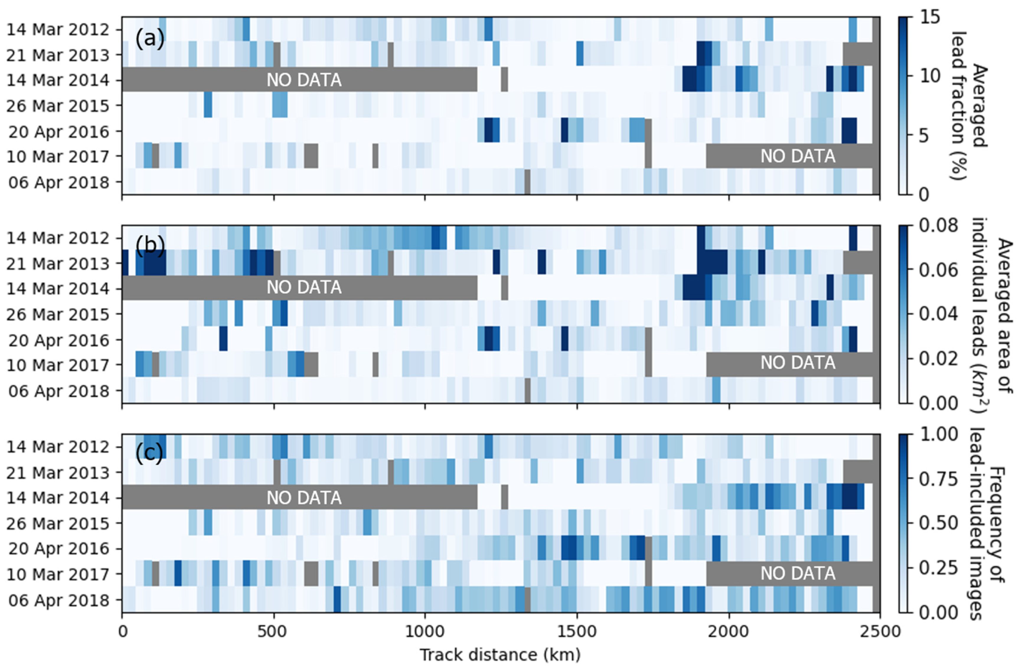
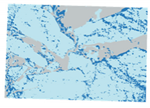
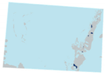
Figure 5a shows the averaged lead fraction for every 25 km along the Laxon Line. Relatively large lead fractions (>15%) were only observed near the Beaufort Sea area (track distance > 1200 km) in 2013, 2014, and 2016, where they were generally located in the FYI region or transition region between FYI and MYI. However, the smaller lead fraction region in the central Arctic (track distance < 1200 km) was primarily covered by MYI and thick ice. Although these observations of one day per year for seven years cannot represent the overall continuous spatiotemporal variations of lead fraction, this general spatial pattern agrees with that of previous lead studies [5,18,19,39]. Figure 5b portrays the averaged area of individual leads for the 25 km track segment, and Figure 5c portrays the ratio of the number of lead-included images to the total number of images for the 25 km segment. The lead fraction (Figure 5a) was determined by the individual lead area (Figure 5b) and the frequency of leads (Figure 5c). For example, although large leads were observed in 2013 for 0–500 km (Figure 5b), lead frequency for this part was low (Figure 5c) due to the small number of large leads. As a result, the averaged lead fraction for this segment was not high because of the low lead frequency. In addition, the lead frequency in 2018 for 1000–2500 km was relatively high, but the averaged lead fraction was not so high due to the large number of small leads.

4.2.2. Retrieval of Freeboard

Based on the DMS lead detection result, we calculated the 400 m mean sea ice freeboard from the ATM surface height data (Figure 6). The MYI area (near central Arctic Ocean) at track distance <1200 km showed a higher freeboard (i.e., thicker ice) compared to that of the FYI area (near the Beaufort Sea with a track distance beyond 1200 km). As shown in Table 7, the FYI area always showed a lower freeboard than the MYI area. In addition, the freeboard retrieved from our lead detection shows a good correlation with the ATM freeboard product provided by NSIDC [32]—correlation coefficient (R) was 0.832, and root mean square difference (RMSD) was 0.105 m (Table 8). It is also noted that 2015, 2016, and 2017 showed relatively lower R and higher root mean square error (RMSE) than the other years (Table 8 and Figure 7), which might be due to the lower classification accuracy of these years (Table 6). Some misclassified leads can make substantial differences in estimation of sea surface height, eventually leading to the differences between our freeboard estimation and the NSIDC freeboard products. Nevertheless, the freeboard differences between MYI and FYI and the cross-validation with the NSIDC freeboard product showed that our lead detection result was reasonable and compatible with other lead detection products.

4.3. Sea Ice Lead Fraction Modelling with Auxiliary Sea Ice Product

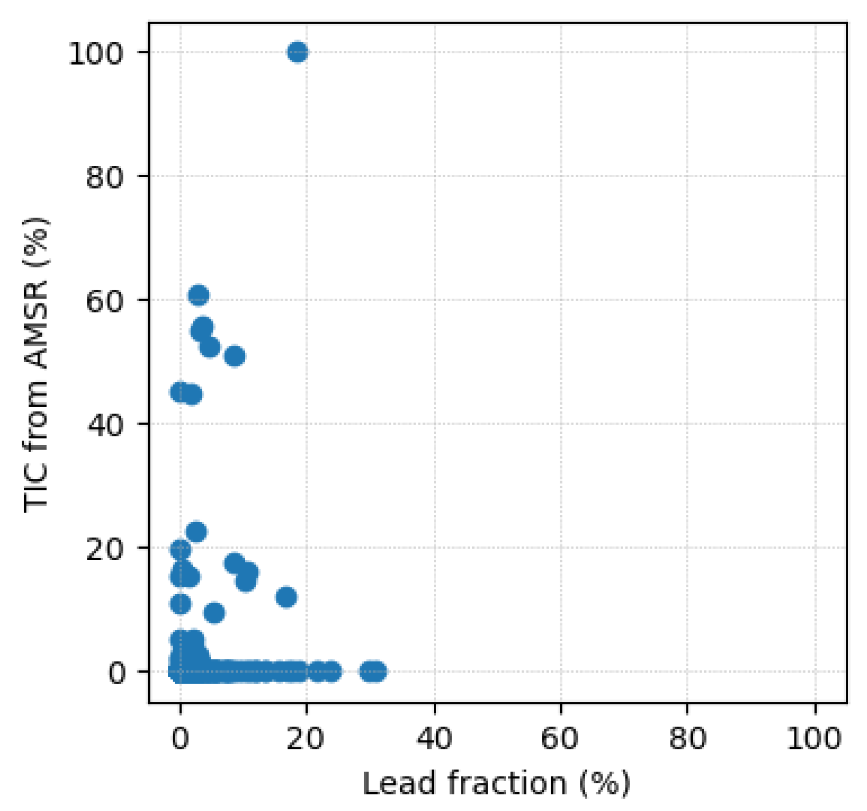
In general, March and April have the lowest lead fraction and lead frequency in a year because of the highly packed sea ice conditions [5,23]. Since the OIB missions were conducted during these months of packed sea ice, the widths of individual observed leads were usually less than 1 km. Indeed, as shown in Figure 5b, most leads had less than 0.1 km2 of area, which accounts for a tiny portion of the entire 25 × 25 km grid cells. Hence, it is reasonable that the DMS-based lead detection and AMSR-based TIC were not highly correlated (R~0.21, Figure 8), because narrow leads are hardly detected by the coarse resolution satellite data [14,40]. For example, we found that most of AMSR-based TIC along the track was zero and AMSR-based SIC was 100% even though the DMS images clearly showed leads in that area.
Figure 9 shows the lead fractions and related dynamic and thermodynamic variables at the scale of 25 km on the same days that DMS images were taken from 2012 to 2018. In general, the lead fractions did not show significant correlation with any single auxiliary variable or kinetic property from sea ice motion data. This is reasonable because (1) these ancillary data have 25 km spatial resolution, which is much coarser than the spatial resolution of the DMS image; (2) the DMS images have only ~500 m of width, representing only a small portion along the Laxon Line; and (3) the formation of sea ice leads results from the accumulative and complex effects of multiple dynamic and thermodynamic variables, rather than just one variable.
Although the DMS images have different spatial scale with the ancillary datasets, we attempted to explore the potential relationship the DMS-based lead fractions and sea ice dynamic and thermodynamic variables from the ancillary datasets. Assuming that (1) these variables are the results of the large-scale atmosphere and ocean circulation and (2) the combination of these variables somehow affects the formation of leads, we normalized all explanatory variables and constructed a series of multiple-variables linear regression models, as shown in Equation (7).
SILF = k = 0 n a k x k
where x k is one of the normalized dynamics-thermodynamic variables, and a k are corresponding coefficients.
The lead fraction variable is the mean of all DMS image-based lead fractions within a 25 km block. On the other hand, all dynamic-thermodynamic variables, including four kinetic moments from the NSIDC sea ice motion data, ERA5 air temperature, and wind velocity data, were averaged by 1, 2, 5, 10, 20, and 30 days prior to the date when the DMS image was taken, considering the accumulative effects of these explanatory variables.
After exploring all possible multiple linear regression models, we found that dynamic-thermodynamic variables integrated by 10 days showed the highest correlation coefficient. Therefore, these explanatory variables were used to reconstruct the linear regression models using the forward and backward stepwise regression approach. The coefficients of all normalized explanatory variables for all models are illustrated in Table 9. There were 11 thermodynamic-dynamic variables, including one thermodynamic variable (temperature), six dynamic variables (velocity of wind and ice motion), and four kinetic moments caused by ice motion.
The forward and backward stepwise regression models for each year identified different sets of explanatory variables. Both 2012 models identified ice motion velocity and divergence as the significant explanatory variables. The 2013 models mainly identified the ice motion velocity and temperature variables. Other than ice motion velocity and temperature, the 2014 models included wind velocity at u-direction, and the correlation coefficient was significantly higher than that of other models. The 2015 models emphasized the functions of wind and ice motion velocity. The 2016 forward model identified more kinetic moments, but the backward model emphasized wind velocity, which represents the possible correlation among these variables. Finally, the 2017 and 2018 models showed significant influence of wind velocity and temperature.
Except for that of 2014, all other models had only moderate correlation, and R2 ranged from 0.26 to 0.66. This was because (1) the sea ice fractions were derived from high spatial resolution DMS images, and the dynamic-thermodynamic variables had a much coarser resolution of 25 km; (2) the atmospheric and oceanic dynamics that contribute to lead formation can occur in a much smaller scale (<25 km scale), which cannot be captured by coarse resolution products; and (3) the uncertainty of the DMS-based lead detection (accuracy of 90%) can be carried and exaggerated in the data fusion and resampling process.
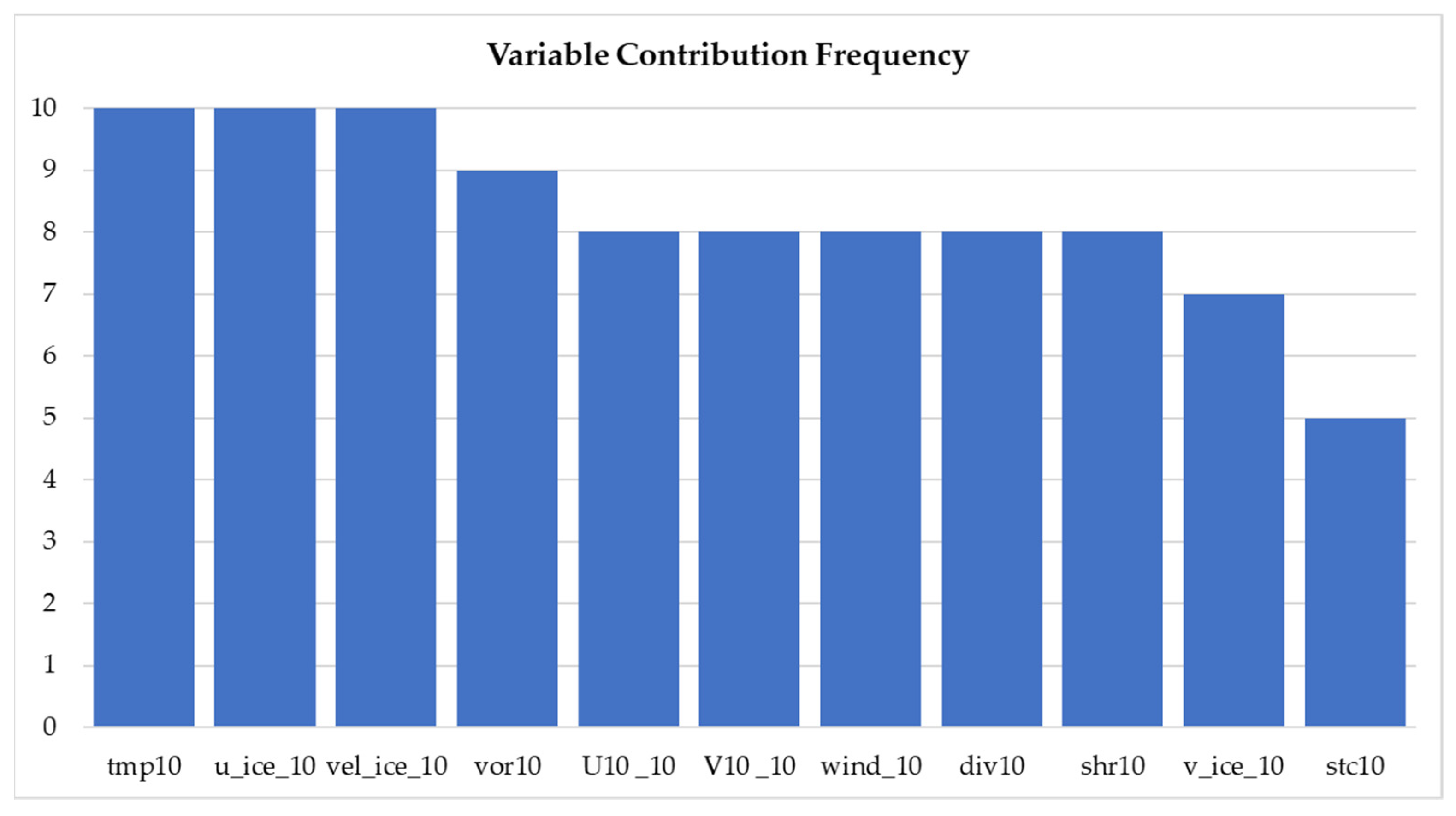
Based on all stepwise regression results, the relative explanatory variable importance could be ranked based on their frequencies in a total of 14 regression models (Table 9), as summarized in Figure 10. It showed that temperature and ice motion vorticity were the leading factors of the formation of sea ice leads, followed by wind vorticity and kinetic moments or tensions of ice motion. However, since this result is only based on stepwise regression of several available variables, it cannot clearly explain the detailed mechanism of lead formation that is a complex combination of multiple ocean and atmospheric parameters. In addition, it is noted that the spatial resolution of the variables can be too coarse to represent the formation of leads in the DMS image scale. Therefore, more comprehensive studies are needed to clearly understand small-scale lead formations in the future.

5. Conclusions

This research demonstrates a scientific case study for sea ice lead detection during 2012–2018 along the IceBridge Laxon Line. To address the lack of standard image processing workflow for sea ice parameter extraction from massive and long-term HSR imagery, a practical object-based image classification workflow was implemented based on the OSSP package to extract multiscale multitype sea ice features and to calculate sea ice lead fractions and freeboard parameters. These sea ice products could be directly used to validate other coarse resolution remote sensing images/products. Furthermore, the high-spatial-resolution sea ice fractions were statistically modeled using large scale dynamic-thermodynamic models.
We found that thick ice, thin ice, water, and shadow could be successfully classified using an object-based classification algorithm or the OSSP package with reasonable overall accuracies of 86.4–96.4%. The sea ice lead fractions along the Laxon Line could be calculated for each DMS image accordingly. The temporal and spatial distribution of leads were verified by ATM surface height data and an independent freeboard product. Finally, the lead fractions were aggregated and modelled with 25 km resolution dynamic and thermodynamic variables including sea ice motion, air temperature, and wind data. All stepwise linear regression models had medium to high correlation coefficients. It seems that temperature and ice motion vorticity were the leading factors of the formation of sea ice leads, and each year could have different dominant factors. The results could provide insightful understanding of the mechanism of sea ice leads, which is useful for climate modelling.
In the future, novel image classification algorithms such as deep learning could be used to improve the traditional machine learning methods. The methods can be extended to other sea ice regions and data types. The results and parameters derived from this study can help the sea ice community to better understand the mechanisms driving sea ice variability so that they can be better represented in climate models.

Author Contributions

Conceptualization, D.S., X.M., H.X. and C.Y.; methodology, D.S., Y.K. and X.M.; software, D.S., A.S. and H.L.; investigation, D.S., Y.K. and X.M.; resources, Q.L. and S.B.; data curation, D.S. and Y.K.; writing—original draft preparation, D.S., Y.K. and X.M.; writing—review and editing, H.X., A.M.M.-N. and C.Y.; project administration, D.S. and X.M.; funding acquisition, C.Y. All authors have read and agreed to the published version of the manuscript.

Funding

This research was funded by NSF with grant numbers 1835507 and 1841520 (GMU), 1835784 (UTSA), 1835512 (MSU), and by NASA with grant numbers 80NSSC18K0843 and 80NSSC19M0194 (UTSA).

Acknowledgments

The authors are thankful to Kevin Wang for providing technical support on testing the online web services and writing the user’s manual. Jennifer Smith proofread the language.

Conflicts of Interest

The authors declare no conflict of interest.

References

  1. Parkinson, C.L. A 40-y record reveals gradual Antarctic sea ice increases followed by decreases at rates far exceeding the rates seen in the Arctic. Proc. Natl. Acad. Sci. USA 2019, 116, 14414–14423. [Google Scholar] [CrossRef] [Green Version]
  2. Peng, G.; Matthews, J.L.; Yu, J.T. Sensitivity Analysis of Arctic Sea Ice Extent Trends and Statistical Projections Using Satellite Data. Remote Sens. 2018, 10, 230. [Google Scholar] [CrossRef] [Green Version]
  3. Marshall, M. Arctic ice low kicks off a cascade of tipping points. New Sci. 2013, 217, 6–7. [Google Scholar] [CrossRef]
  4. Parkinson, C.L.; Comiso, J.C. On the 2012 record low Arctic sea ice cover: Combined impact of preconditioning and an August storm. Geophys. Res. Lett. 2013, 40, 1356–1361. [Google Scholar] [CrossRef]
  5. Wang, Q.; Danilov, S.; Jung, T.; Kaleschke, L.; Wernecke, A. Sea ice leads in the Arctic Ocean: Model assessment, interannual variability and trends. Geophys. Res. Lett. 2016, 43, 7019–7027. [Google Scholar] [CrossRef] [Green Version]
  6. Hui, F.; Zhao, T.; Li, X.; Shokr, M.; Heil, P.; Zhao, J.; Zhang, L.; Cheng, X. Satellite-Based Sea Ice Navigation for Prydz Bay, East Antarctica. Remote Sens. 2017, 9, 518. [Google Scholar] [CrossRef] [Green Version]
  7. Hakkinen, S.; Proshutinsky, A.; Ashik, I. Sea ice drift in the Arctic since the 1950s. Geophys. Res. Lett. 2008, 35, 19704. [Google Scholar] [CrossRef] [Green Version]
  8. Hirano, D.; Fukamachi, Y.; Watanabe, E.; Ohshima, K.I.; Iwamoto, K.; Mahoney, A.R.; Eicken, H.; Simizu, D.; Tamura, T. A wind-driven, hybrid latent and sensible heat coastal polynya off Barrow, Alaska. J. Geophys. Res. Ocean. 2016, 121, 980–997. [Google Scholar] [CrossRef] [Green Version]
  9. Alam, A. Determination of surface turbulent fluxes over leads in Arctic sea ice. J. Geophys. Res. C Ocean. 1997, 102, 3331–3343. [Google Scholar] [CrossRef]
  10. Andreas, E.L.; Murphy, B. Bulk Transfer Coefficients for Heat and Momentum over Leads and Polynyas. J. Phys. Oceanogr. 1986, 16, 1875–1883. [Google Scholar] [CrossRef] [Green Version]
  11. Marcq, S.; Weiss, J. Influence of sea ice lead-width distribution on turbulent heat transfer between the ocean and the atmosphere. Cryosphere 2012, 6, 143–156. [Google Scholar] [CrossRef] [Green Version]
  12. Worby, A.P.; Allison, I. Ocean-atmosphere energy exchange over thin, variable concentration Antarctic pack ice. Ann. Glaciol. 1991, 15, 184–190. [Google Scholar] [CrossRef] [Green Version]
  13. Maykut, G.A. Large-scale heat exchange and ice production in the central Arctic. J. Geophys. Res. 1982, 87, 7971. [Google Scholar] [CrossRef]
  14. Röhrs, J.; Kaleschke, L. An algorithm to detect sea ice leads by using AMSR-E passive microwave imagery. Cryosphere 2012, 6, 343–352. [Google Scholar] [CrossRef] [Green Version]
  15. Heorton, H.D.B.S.; Radia, N.; Feltham, D.L. A Model of Sea Ice Formation in Leads and Polynyas. J. Phys. Oceanogr. 2017, 47, 1701–1718. [Google Scholar] [CrossRef]
  16. National Research Council. Earth Science and Applications from Space: National Imperatives for the Next Decade and Beyond; National Academies Press: Washington, DC, USA, 2007. [Google Scholar]
  17. Hall, D.K.; Riggs, G.A.; Salomonson, V.V. MODIS Snow and Sea Ice Products. In Earth Science Satellite Remote Sensing; Springer: Berlin/Heidelberg, Germany, 2006; pp. 154–181. [Google Scholar]
  18. Willmes, S.; Heinemann, G. Sea-Ice Wintertime Lead Frequencies and Regional Characteristics in the Arctic, 2003–2015. Remote Sens. 2016, 8, 4. [Google Scholar] [CrossRef] [Green Version]
  19. Hoffman, J.; Ackerman, S.; Liu, Y.; Key, J. The Detection and Characterization of Arctic Sea Ice Leads with Satellite Imagers. Remote Sens. 2019, 11, 521. [Google Scholar] [CrossRef] [Green Version]
  20. Lindsay, R.W.; Rothrock, D.A. Arctic sea ice leads from advanced very high resolution radiometer images. J. Geophys. Res. 1995, 100, 4533. [Google Scholar] [CrossRef]
  21. Li, L.; Changqing, K.E.; Xie, H.; Ruibo, L.; Anqi, T. Aerial observations of sea ice and melt ponds near the North Pole during CHINARE2010. Acta Oceanol. Sin. 2017, 36, 64–72. [Google Scholar] [CrossRef]
  22. Sha, D.; Miao, X.; Xu, M.; Yang, C.; Xie, H.; Mestas-Nuñez, A.M.; Li, Y.; Liu, Q.; Yang, J. An On—Demand Service for Managing and Analyzing Arctic Sea Ice High Spatial Resolution Imagery. Data 2020, 5, 39. [Google Scholar] [CrossRef] [Green Version]
  23. Onana, V.-D.-P.; Kurtz, N.T.; Farrell, S.L.; Koenig, L.S.; Studinger, M.; Harbeck, J.P. A Sea-Ice Lead Detection Algorithm for Use With High-Resolution Airborne Visible Imagery. IEEE Trans. Geosci. Remote Sens. 2013, 51, 38–56. [Google Scholar] [CrossRef]
  24. Miao, X.; Xie, H.; Ackley, S.F.; Perovich, D.K.; Ke, C. Object-based detection of Arctic sea ice and melt ponds using high spatial resolution aerial photographs. Cold Reg. Sci. Technol. 2015, 119, 211–222. [Google Scholar] [CrossRef]
  25. Wright, N.C.; Polashenski, C.M. Open-source algorithm for detecting sea ice surface features in high-resolution optical imagery. Cryosphere 2018, 12, 1307–1329. [Google Scholar] [CrossRef] [Green Version]
  26. Wright, N.C.; Polashenski, C.M.; Mcmichael, S.T.; Beyer, R.A. Observations of sea ice melt from Operation IceBridge imagery. Cryosphere 2020, 14, 3523–3536. [Google Scholar] [CrossRef]
  27. Dominguez, R. IceBridge DMS L1B Geolocated and Orthorectified Images; National Snow and Ice Data Center: Boulder, CO, USA, 2010. [Google Scholar]
  28. Markus, T.; Comiso, J.C.; Meier, W.N. AMSR-E/AMSR2 Unified L3 Daily 25 km Brightness Temperatures & Sea Ice Concentration Polar Grids, Version 1; NASA National Snow and Ice Data Center Distributed Active Archive Center: Boulder, CO, USA, 2018. [Google Scholar]
  29. Meier, W.N.; Markus, T.; Comiso, J.; Ivanoff, A.; Miller, J. Amsr2 Sea Ice Algorithm Theoretical Basis Document; NASA Goddard Space Flight Center: Greenbelt, MD, USA, 2017. [Google Scholar]
  30. Markus, T.; Cavalieri, D.J. An enhancement of the NASA Team sea ice algorithm. IEEE Trans. Geosci. Remote Sens. 2000, 38, 1387–1398. [Google Scholar] [CrossRef] [Green Version]
  31. Markus, T.; Cavalieri, D. The AMSR-E NT2 Sea Ice Concentration Algorithm: Its Basis and Implementation. J. Remote Sens. Soc. Jpn. 2009, 29, 216–225. [Google Scholar] [CrossRef]
  32. Kurtz, N.T.; Farrell, S.L.; Studinger, M.; Galin, N.; Harbeck, J.P.; Lindsay, R.; Onana, V.D.; Panzer, B.; Sonntag, J.G. Sea ice thickness, freeboard, and snow depth products from Operation IceBridge airborne data. Cryosphere 2013, 7, 1035–1056. [Google Scholar] [CrossRef] [Green Version]
  33. Wang, X.; Guan, F.; Liu, J.; Xie, H.; Ackley, S. An improved approach of total freeboard retrieval with IceBridge Airborne Topographic Mapper (ATM) elevation and Digital Mapping System (DMS) images. Remote Sens. Environ. 2016, 184, 582–594. [Google Scholar] [CrossRef] [Green Version]
  34. Tschudi, M.; Meier, W.N.; Stewart, J.S.; Fowler, C.; Maslanik, J. Polar Pathfinder Daily 25 km EASE-Grid Sea Ice Motion Vectors, Version 4; NASA National Snow and Ice Data Center Distributed Active Archive Center: Boulder, CO, USA, 2019. [Google Scholar] [CrossRef]
  35. Aaboe, S.; Down, E.J.; Eastwood, S. Product User Manual for the Global Sea-Ice Edge and Type Product; Norwegian Meteorological Institute: Oslo, Norway, 2021. [Google Scholar]
  36. NSIDC. IceBridge Sea Ice Freeboard, Snow Depth, and Thickness Quick Look, Version 1. Available online: https://nsidc.org/data/NSIDC-0708/versions/1 (accessed on 16 September 2021).
  37. Molinari, R.; Kirwan, A.D. Calculations of Differential Kinematic Properties from Lagrangian Observations in the Western Caribbean Sea. J. Phys. Oceanogr. 1975, 5, 483–491. [Google Scholar] [CrossRef]
  38. Wilkinson, L. Tests of significance in stepwise regression. Psychol. Bull. 1979, 86, 168–174. [Google Scholar] [CrossRef]
  39. Qu, M.; Pang, X.; Zhao, X.; Lei, R.; Ji, Q.; Liu, Y.; Chen, Y. Spring leads in the Beaufort Sea and its interannual trend using Terra/MODIS thermal imagery. Remote Sens. Environ. 2021, 256, 112342. [Google Scholar] [CrossRef]
  40. Lee, S.; Kim, H.; Im, J. Arctic lead detection using a waveform mixture algorithm from CryoSat-2 data. Cryosphere 2018, 12, 1665–1679. [Google Scholar] [CrossRef] [Green Version]
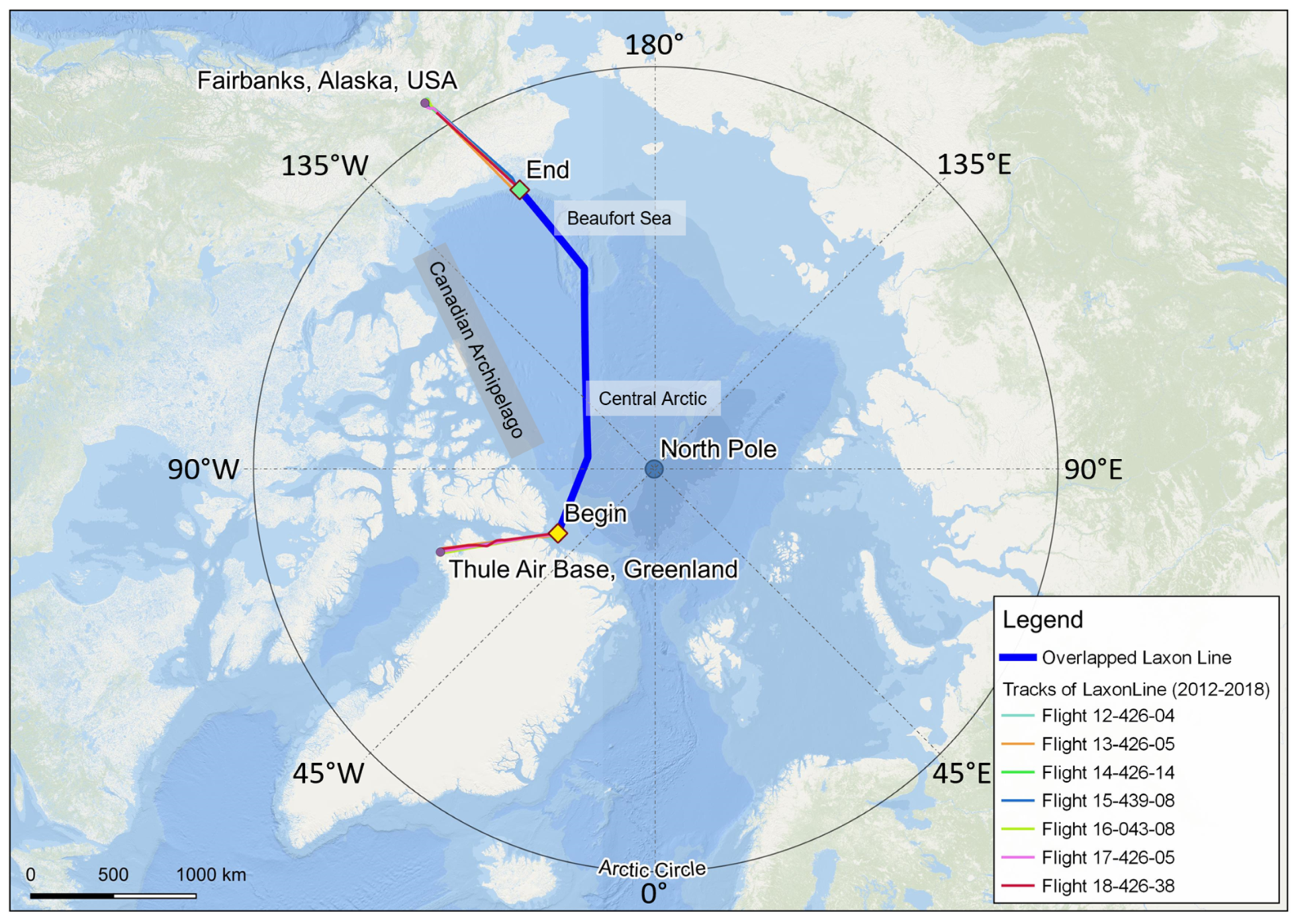
Figure 1. Spatial distribution of the seven tracks along the Laxon Line from 2012 to 2018. The tracks are highly overlapped.
Remotesensing 13 04177 g001
Figure 2. Sea ice lead detection workflow.
Remotesensing 13 04177 g002
Figure 3. DMS sea ice sample images in 2012 were classified into three subgroups based on different lighting conditions.
Remotesensing 13 04177 g003
Figure 4. Data fusion diagram with derived geophysical parameters and DMS-based sea ice leads (each 25 km AMSR pixel covers around 5–70 point of HSR image locations).
Remotesensing 13 04177 g004
Figure 5. (a) Averaged lead fraction for every 25 km; (b) averaged area of individual leads for every 25 km; (c) frequency of lead-included images for every 25 km. Gray parts indicate missing/invalid data.
Remotesensing 13 04177 g005
Figure 6. Averaged ATM freeboard for every 25 km for each year.
Remotesensing 13 04177 g006
Figure 7. Scatter plot between ATM freeboard derived by our lead detection and NSIDC freeboard product for every 400 m (2% random selection of the total points).
Remotesensing 13 04177 g007
Figure 8. Scatter plot between DMS-based lead fraction (this study) and AMSR-based TIC.
Remotesensing 13 04177 g008
Figure 9. (a) DMS-based lead fraction and nearby ice types; (b) ERA5 air temperature; (c) ERA5 wind velocity; (d) sea ice motion for each year.
Remotesensing 13 04177 g009
Figure 10. Relative importance of dynamic-thermodynamic explanatory variables.
Remotesensing 13 04177 g010
Table 1. The DMS images selected for lead detection along the Laxon Line from 2012 to 2018.
NameDateImage ## Image with Sea Ice LeadsSelected/Original Image Size (GB)Lighting Condition
Flight 12-426-0414 March 201216,544106614.8/260Cloudy
Flight 13-426-0521 March 201318,48099313.8/290Normal
Flight 14-426-1414 March 201414,3224925.2/150Cloudy
Flight 15-439-0826 March 201520,0388169.3/250Normal
Flight 16-043-0820 April 201615,205106918.4/270Normal
Flight 17-426-0510 March 201710,9396598.67/93Cloudy
Flight 18-426-386 April 201811,146104022.2/240Normal
Table 2. Auxiliary sea ice datasets.
Product NameTypeSourceSpatial ResolutionCategory
AMSR-E/AMSR2 Unified L3 Daily Brightness Temperatures & Sea Ice ConcentrationPassive microwaveNSIDC25 kmSea Ice
IceBridge Airborne Topographic Mapper (ATM)Laser altimeterNSIDC~1 m footprint (resampled to 2 m grid)Sea Ice
Global sea ice typeSea ice typeEUMETSAT OSI SAF10 kmSea Ice
Polar Pathfinder Daily EASE-Grid Sea Ice Motion VectorsSea ice motionNSIDC25 kmDynamic
ERA5 (air temperature
and wind velocity)
Climate reanalysisEuropean Centre for Medium-Range Weather Forecasts (ECMWF)0.25°Dynamic and thermodynamic
Table 3. The DMS images selected for lead detection in the Laxon Line from 2012 to 2018.
Testing Group# Training Image# Training Object# Test Image# Test object
DMS2012_normal6505114
DMS2012_medium790594
DMS2012_ poor7655124
DMS2013131967221
DMS2014_normal81066178
DMS2014_medium6666119
DMS2015111509254
DMS2016814412444
DMS2017121406150
DMS2018131359319
Table 4. Variables for the multiple linear regression models.
DepartmentFactorsDescription
Sea Ice Leadsmean_leadsMean lead fraction for 25 km segment
TemperaturetmpXXAveraged air temperature for last XX days (e.g., tmp03 means average temperature of last 1, 2, 3 days)
WindU10_XXAveraged u-component of wind velocity for last XX days
V10_XXAveraged v-component of wind velocity for last XX days
wind_XXAveraged wind velocity for last XX days (e.g., wind_10 means wind velocity for last 10 days)
Sea Ice Motionu_ice_XXAveraged u-component of ice velocity for last XX days (e.g., u_ice_10 means u-velocity for last 10 days)
v_ice_XXAveraged v-component of ice velocity for last XX days (e.g., v_ice_10 means v-velocity for last 10 days)
vel_ice_XXAveraged ice velocity for last XX days (e.g., v_ice_10 means ice velocity for last 10 days)
divXXAveraged divergence of sea ice motion for last XX days (e.g., div10 means divergence for last 10 days)
vorXXAveraged vorticity of sea ice motion for last XX days (e.g., vor10 means vorticity for last 10 days)
shrXXAveraged shearing deformation of sea ice motion for last XX days (e.g., shr10 means shearing deformation for last 10 days)
stcXXAveraged stretching deformation of sea ice motion for last XX days (e.g., stc10 means stretching deformation for last 10 days)
Table 5. Comparison of original 2012 DMS images and classified results for three subgroups. Two samples were selected for each subgroup.
Sample Result 1Sample Result 2
Raw ImageClassified ResultRaw ImageClassified Result
Normal Remotesensing 13 04177 i001 Remotesensing 13 04177 i002 Remotesensing 13 04177 i003 Remotesensing 13 04177 i004
Medium Remotesensing 13 04177 i005 Remotesensing 13 04177 i006 Remotesensing 13 04177 i007 Remotesensing 13 04177 i008
Poor Remotesensing 13 04177 i009 Remotesensing 13 04177 i010 Remotesensing 13 04177 i011 Remotesensing 13 04177 i012
Remotesensing 13 04177 i013
Table 6. Pixel-level classification accuracy for each production group. All values except Kappa coefficient are in percentages.
Testing GroupOverall
Accuracy
Kappa Coef.UA_Thick **UA_ThinUA_ShadowUA_WaterPA_Thick **PA_ThinPA_ShadowPA_Water
DMS2012_normal88.90.8388.091.783.8nan *98.494.263.8nan
DMS2012_medium93.60.8597.385.0nan95.593.893.1nan97.5
DMS2012_poor93.80.8695.096.0nan61.998.981.2nan94.9
DMS201396.40.9592.2100.099.495.599.796.588.399.9
DMS2014_normal88.00.8274.786.293.998.097.181.399.789.0
DMS2014_medium93.70.8991.796.3nan97.1100.075.7nan97.1
DMS201586.40.7886.683.598.693.499.880.982.257.9
DMS201687.90.8382.189.395.095.799.468.889.790.2
DMS201786.70.7587.482.8nan99.497.676.5nan60.7
DMS201893.50.8891.996.595.297.998.579.189.498.4
Average Accuracy90.90.8488.790.794.392.798.382.785.587.3
*,** User’s accuracy and producer’s accuracy for each classified ice type represented as UA_XX, and PA_XX, and XX could be thick ice, thin ice, shadow, or open water.
Table 7. ATM sea ice freeboard retrieved from the DMS lead detection.
YearFYIMYITotal
20130.263 0.519 0.409
20140.277 0.339 0.320
20150.275 0.470 0.407
20160.3350.398 0.354
20170.211 0.467 0.366
20180.320 0.505 0.414
Table 8. R and RMSE between our freeboard estimation and NSIDC freeboard estimation.
YearRRMSD (m)
20130.9280.089
20140.9070.063
20150.7550.140
20160.7840.114
20170.7420.119
20180.8690.082
Total0.8320.105
Table 9. Selected variables and coefficients in 14 stepwise linear regressions.
YearApproachR2Tmp10U10_10V10 _10Wind_10U_Ice_10V_Ice_10Vel_Ice_10Div10Vor10Shr10Stc10Constant
2012Forward0.26////−0.39−0.380.16−0.10−0.08//0.41
Backward0.260.10///−0.34−0.19/−0.12///0.31
2013Forward0.48−1.19//0.35−6.46−2.789.51/−0.01−0.14/0.60
Backward0.48−1.18//0.35−6.44−2.759.45//−0.15/0.08
2014Forward0.874.61−5.60−0.971.091.2415.31−12.98/0.89−0.55/−2.08
Backward0.874.64−5.37//1.1613.34−11.25−0.160.87−0.59/−1.94
2015Forward0.34//−0.53/−1.35/1.190.150.140.28−0.330.40
Backward0.34//−0.53/−1.35/1.190.150.140.28−0.330.40
2016Forward0.29/−0.79////0.290.30−0.390.570.150.21
Backward0.340.67−4.62−0.534.09////−0.360.46/0.22
2017Forward0.66−1.17−6.54−3.086.772.98−0.09−2.01−0.19///1.50
Backward0.66−1.15−6.57−3.116.863.02/−2.09−0.19///1.45
2018Forward0.300.34−1.40−1.401.83////−0.03/−0.310.45
Backward0.300.34−1.31−1.331.72//////−0.320.42
Publisher’s Note: MDPI stays neutral with regard to jurisdictional claims in published maps and institutional affiliations.