
Application of Optical Flow Technique and Photogrammetry for Rockfall Dynamics: A Case Study on a Field Test


Abstract
:
1. Introduction
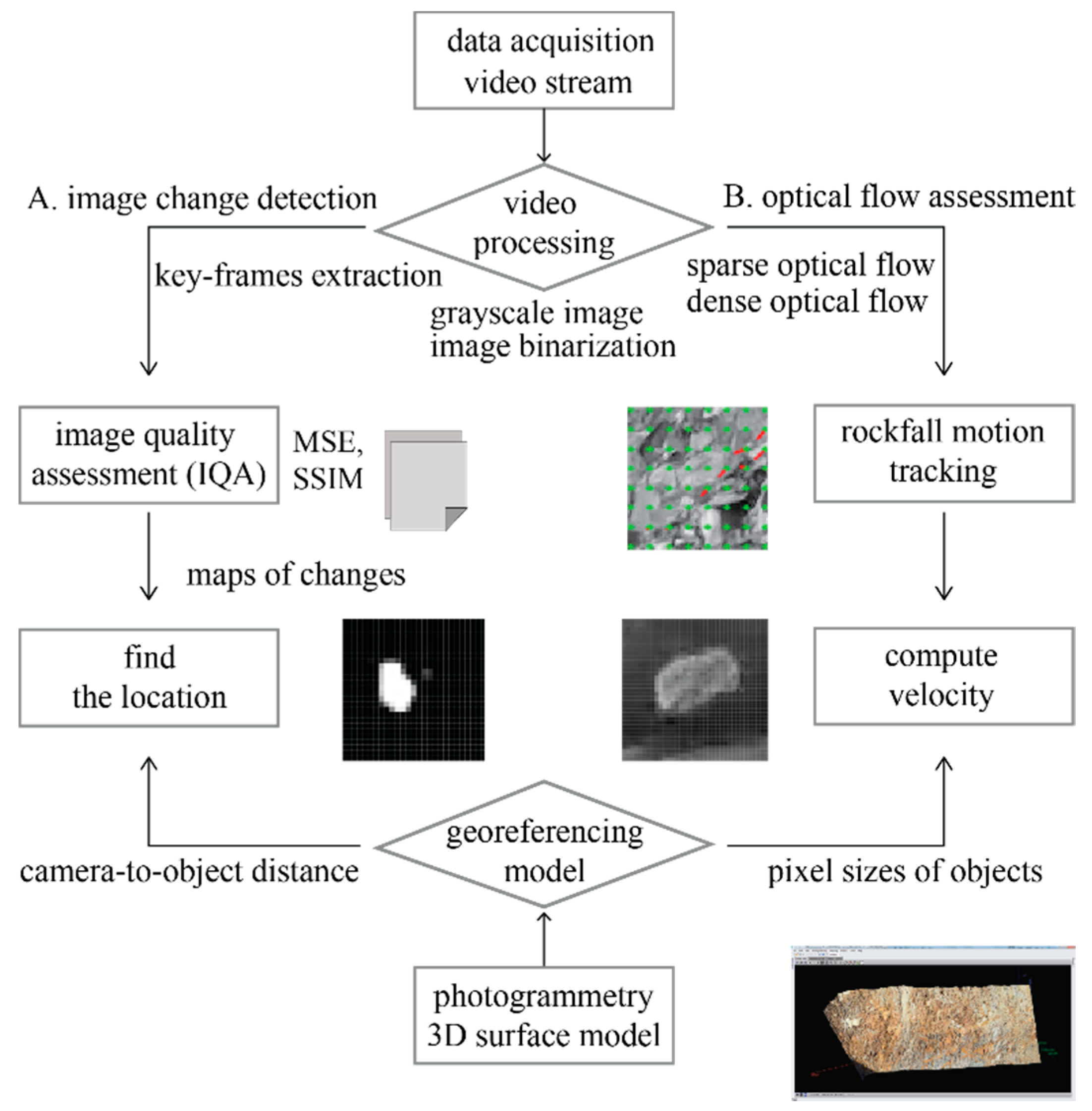
2. Methods
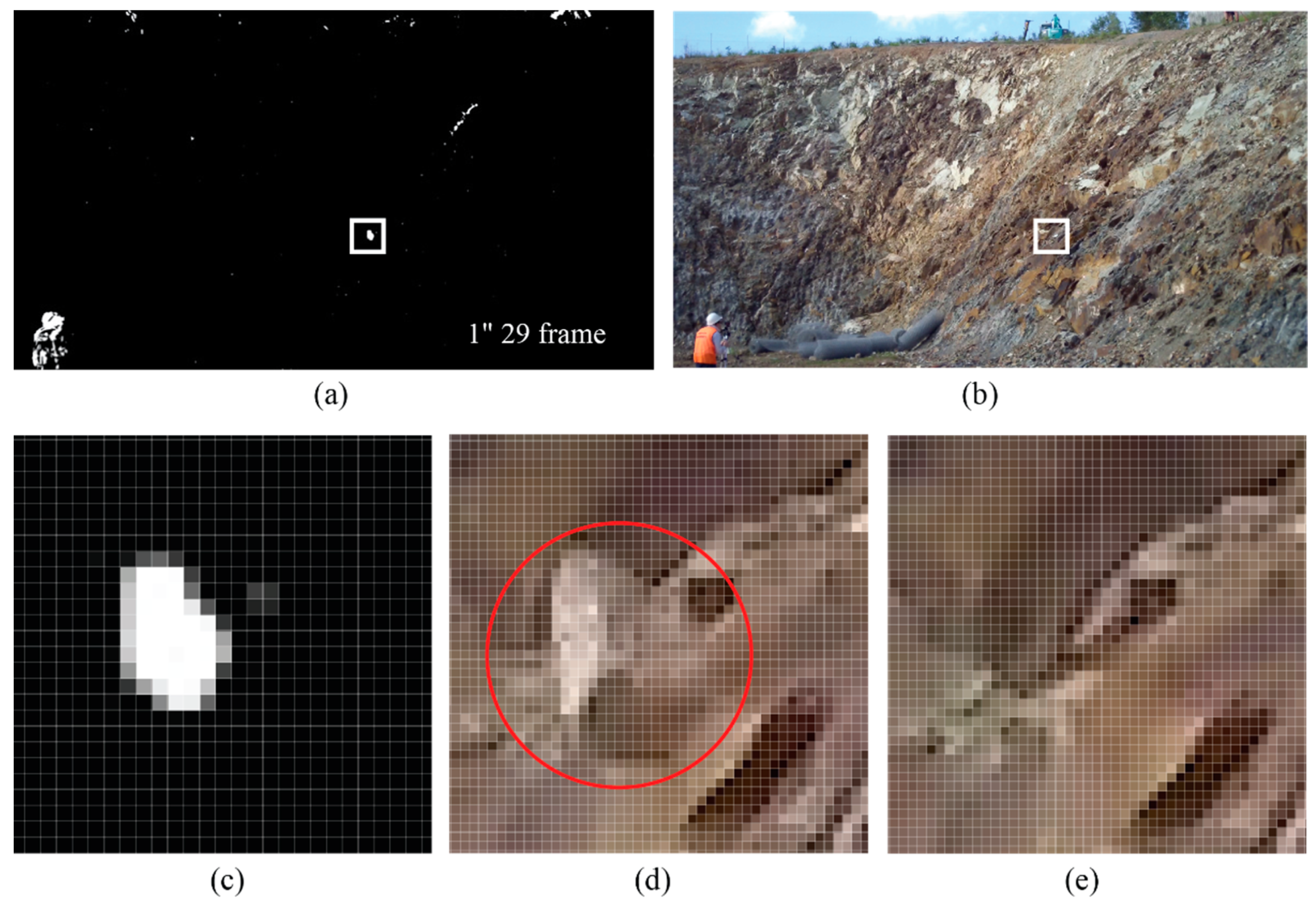
2.1. Image Change Detection Using Time-Lapse Image
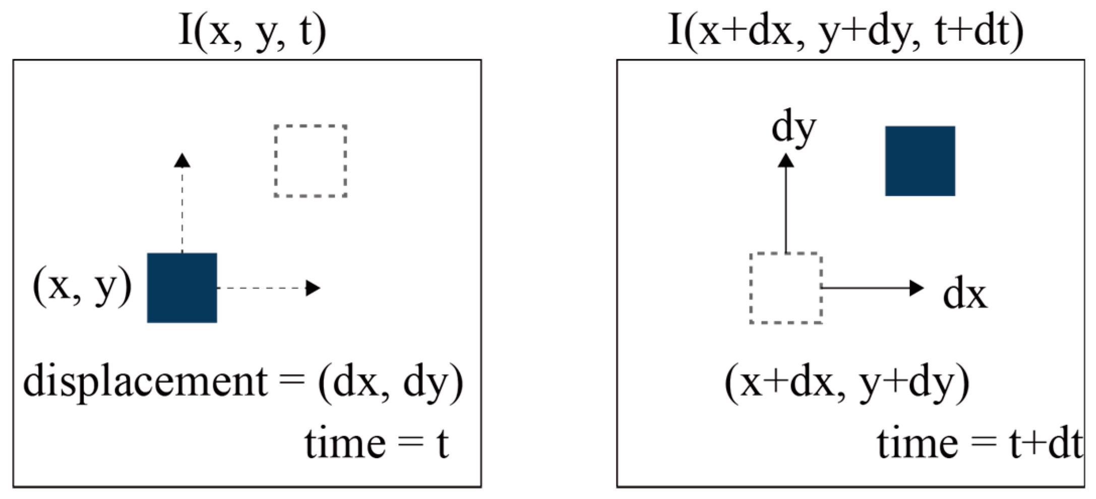
2.2. Optical Flow
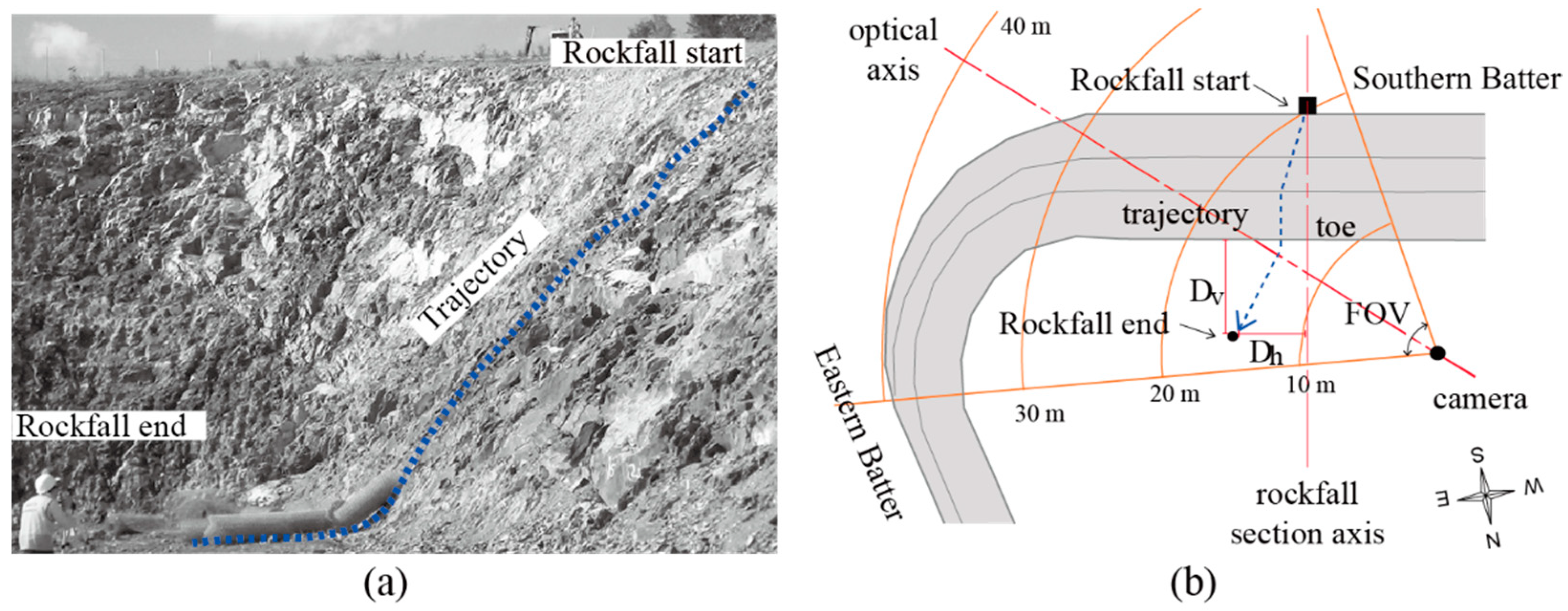
3. Data Collection
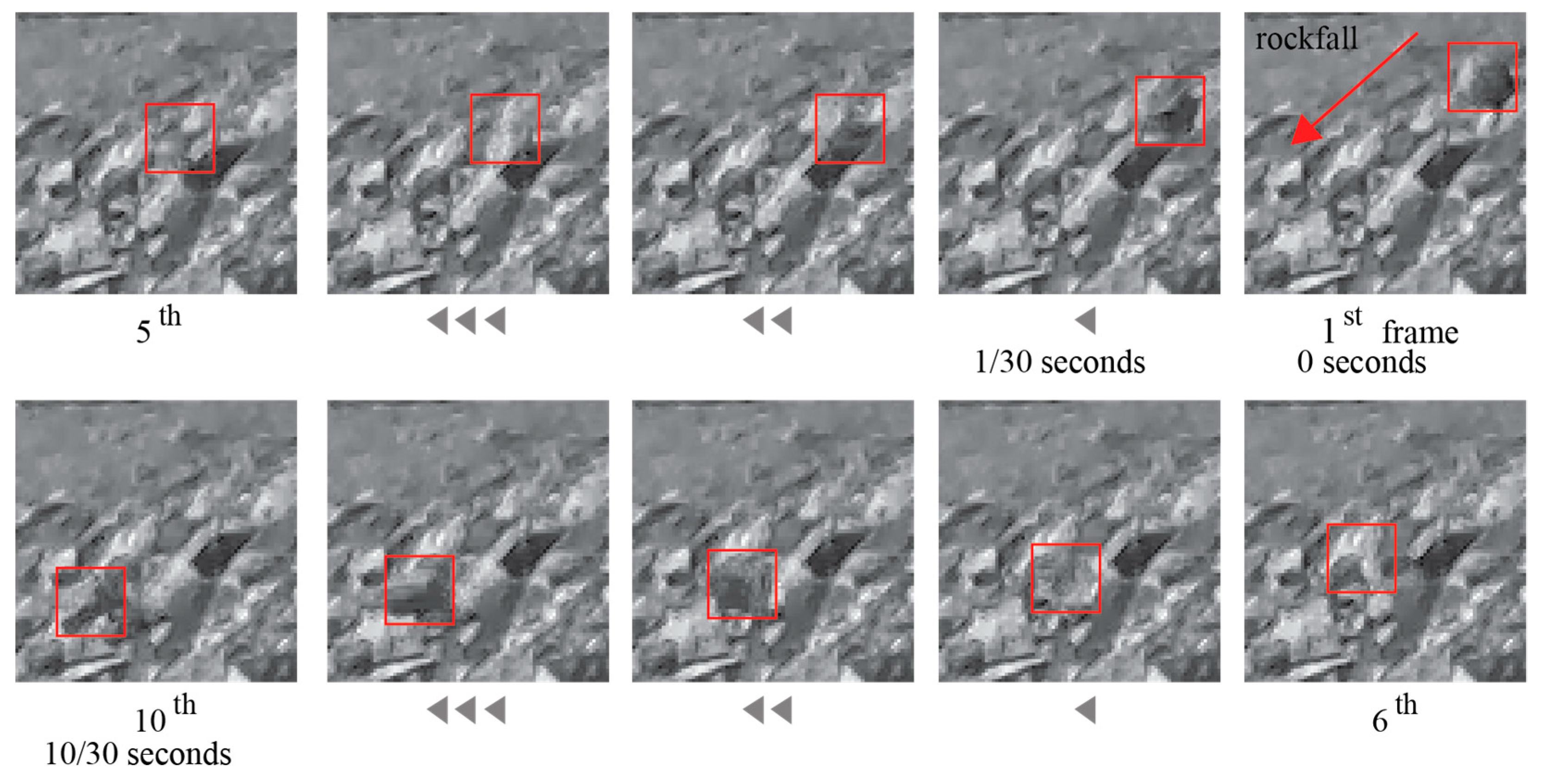
3.1. Video Capturing and Data Sampling
3.2. Dataset Evaluation
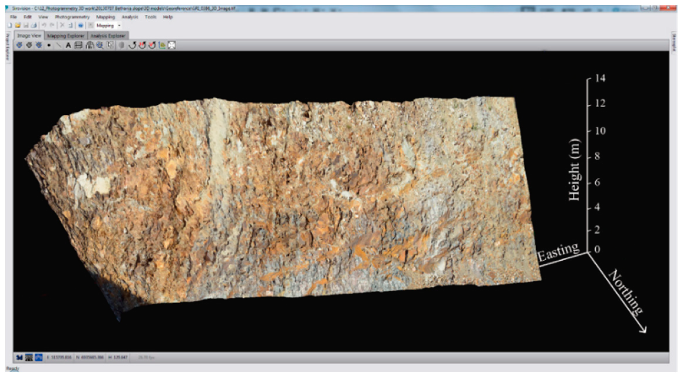
3.3. Photogrammetry
4. Results
4.1. Image Quality Assessment
4.1.1. Visualization by Error Map
4.1.2. MSE and SSIM
4.2. Optical Flow Assessment
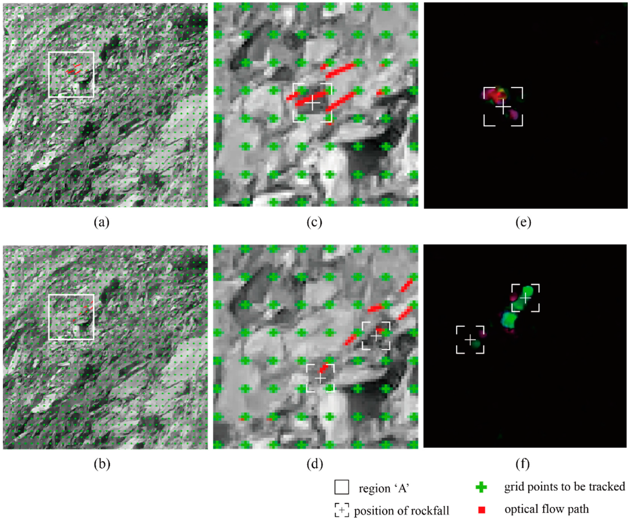
4.2.1. Sparse Optical Flow
4.2.2. Dense Optical Flow
5. Discussion
5.1. Tracking of Rockfall by Sparse Optical Flow
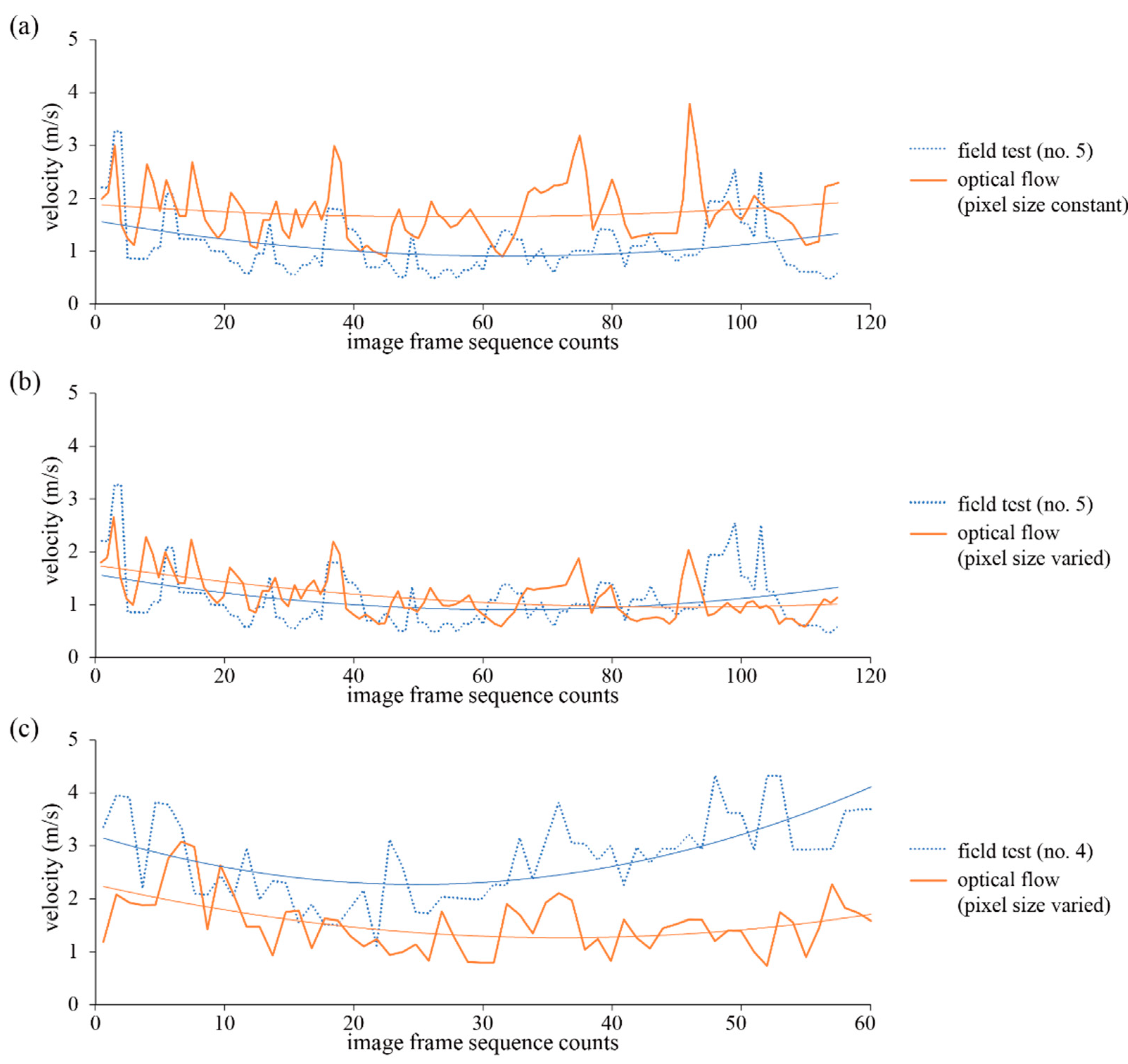
5.2. Estimation of Rockfall Motion from Dense Optical Flow
6. Conclusions
Author Contributions
Funding
Institutional Review Board Statement
Informed Consent Statement
Data Availability Statement
Conflicts of Interest
References
- Dick, D.J.; Eberhardt, E.; Stead, D.; Rose, N.D. Early detection of impending slope failure in open pit mines using spatial and temporal analysis of real aperture radar measurements. In Proceedings of the Slope Stability 2013, Brisbane, QLD, Australia, 25–27 September 2013; Australian Centre for Geomechanics: Crawley, Australia, 2013; pp. 949–962. [Google Scholar]
- Intrieri, E.; Gigli, G.; Mugnai, F.; Fanti, R.; Gasagli, N. Design and implementation of a landslide early warning system. Eng. Geol. 2012, 147–148, 124–136. [Google Scholar] [CrossRef] [Green Version]
- Brideau, M.A.; Sturzenegger, M.; Stead, D.; Jaboyedoff, M.; Lawrence, M.; Roberts, N.; Ward, B.; Millard, T.; Clague, J. Stability analysis of the 2007 Chehalis Lake landslide based on long-range terrestrial photogrammetry and airborne LiDAR data. Landslides 2012, 9, 75–91. [Google Scholar] [CrossRef]
- Park, S.; Lim, H.; Tamang, B.; Jin, J.; Lee, S.; Chang, S.; Kim, Y. A study on the slope failure monitoring of a model slope by the application of a displacement sensor. J. Sens. 2019, 2019, 7570517. [Google Scholar] [CrossRef]
- Donovan, J.; Raza Ali, W. A change detection method for slope monitoring and identification of potential rockfall using three-dimensional imaging. In Proceedings of the 42nd US Rock Mechanics Symposium and 2nd U.S.-Canada Rock Mechanics Symposium, San Francisco, CA, USA, 29 June–2 July 2008. [Google Scholar]
- Kim, D.H.; Gratchev, I.; Balasubramaniam, A.S. Determination of joint roughness coefficient (JRC) for slope stability analysis: A case study from the Gold Coast area. Landslides 2013, 10, 657–664. [Google Scholar] [CrossRef] [Green Version]
- Fantini, A.; Fiorucci, M.; Martino, S. Rock falls impacting railway tracks: Detection analysis through an artificial intelligence camera prototype. Wirel. Commun. Mob. Comput. 2017, 2017, 9386928. [Google Scholar] [CrossRef] [Green Version]
- Kromer, R.; Walton, G.; Gray, B.; Lato, M.; Group, R. Development and optimization of an automated fixed-location time lapse photogrammetric rock slope monitoring system. Remote Sens. 2019, 11, 1890. [Google Scholar] [CrossRef] [Green Version]
- Li, Q.; Min, G.; Chen, P.; Liu, Y.; Tian, S.; Zhang, D.; Zhang, W. Computer vision-based techniques and path planning strategy in a slope monitoring system using unmanned aerial vehicle. Int. J. Adv. Robot. Syst. 2020, 17. [Google Scholar] [CrossRef]
- Voumard, J.; Abellán, A.; Nicolet, P.; Penna, I.; Chanut, M.-A.; Derron, M.-H.; Jaboyedoff, M. Using street view imagery for 3-D survey of rock slope failures. Nat. Hazards Earth Syst. Sci. 2017, 17, 2093–2107. [Google Scholar] [CrossRef] [Green Version]
- Ghorbanzadeh, O.; Meena, S.R.; Blaschke, T.; Aryal, J. UAV-based slope failure detection using deep-learning convolutional neural networks. Remote Sens. 2019, 11, 2046. [Google Scholar] [CrossRef] [Green Version]
- McHuge, E.L.; Girard, J.M. Evaluating techniques for monitoring rockfalls and slope stability. In Proceedings of the 21st International Conference on Ground Control in Mining, Morgantown, WV, USA, 6–8 August 2002; West Virginia University: Monongalia County, WV, USA, 2002; pp. 335–343. [Google Scholar]
- Kim, D.; Balasubramaniam, A.S.; Gratchev, I.; Kim, S.R.; Chang, S.H. Application of image quality assessment for rockfall investigation. In Proceedings of the 16th Asian Regional Conference on Soil Mechanics and Geotechnical Engineering, Taipei, Taiwan, 14–18 October 2019. [Google Scholar]
- Lu, D.; Mausel, P.; Brondizizio, E.; Moran, E. Change detection techniques. Int. J. Remote Sens. 2004, 25, 2365–2407. [Google Scholar] [CrossRef]
- Srokosz, P.E.; Bujko, M.; Bochenska, M.; Ossowski, R. Optical flow method for measuring deformation of soil specimen subjected to torsional shearing. Measurement 2021, 174, 109064. [Google Scholar] [CrossRef]
- Kenji, A.; Teruo, Y.; Hiroshi, H. Landslide occurrence prediction using optical flow. In Proceedings of the 2019 19th International Conference on Control, Automation and Systems (ICCAS), Jeju, Korea, 15–18 October 2019; pp. 1311–1315. [Google Scholar]
- Rosin, P.L.; Hervás, J. Remote sensing image thresholding methods for determining landslide activity. Int. J. Remote Sens. 2005, 26, 1075–1092. [Google Scholar] [CrossRef] [Green Version]
- Khan, M.W.; Dunning, S.; Bainbridge, R.; Martin, J.; Diaz-Moreno, A.; Torun, H.; Jin, N.; Woodward, J.; Lim, M. Low-cost automatic slope monitoring using vector tracking analyses on live-streamed time-lapse imagery. Remote Sens. 2021, 13, 893. [Google Scholar] [CrossRef]
- Vanneschi, C.; Camillo, M.D.; Aiello, E.; Bonciani, F.; Salvini, R. SfM-MVS photogrammetry for rockfall analysis and hazard assessment along the ancient Roman via Flaminia road at the Furlo Gorge (Italy). ISPRS Int. J. Geo-Inf. 2019, 8, 325. [Google Scholar] [CrossRef] [Green Version]
- Kim, D.H.; Gratchev, I.; Berends, J.; Balasubramaniam, A.S. Calibration of restitution coefficients using rockfall simulations based on 3D photogrammetry model: A case study. Nat. Hazards. 2015, 78, 1931–1946. [Google Scholar] [CrossRef] [Green Version]
- Štroner, M.; Urban, R.; Reindl, T.; Seidl, J.; Broucek, J. Evaluation of the georeferencing accuracy of a photogrammetric model using a quadrocopter with onboard GNSS RTK. Sensors 2020, 20, 2318. [Google Scholar] [CrossRef] [PubMed] [Green Version]
- Yuan, W.; Yuan, X.; Xu, S.; Gong, J.; Shibasaki, R. Dense image-matching via optical flow field estimation and fast-guided filter refinement. Remote Sens. 2019, 11, 2410. [Google Scholar] [CrossRef] [Green Version]
- Nones, M.; Archetti, R.; Guerrero, M. Time-Lapse photography of the edge-of-water line displacements of a sandbar as a proxy of riverine morphodynamics. Water 2018, 10, 617. [Google Scholar] [CrossRef] [Green Version]
- Li, L.; Leung, M. Integrating intensity and texture differences for robust change detection. IEEE Trans. Image Process. 2002, 11, 105–112. [Google Scholar]
- Chandler, D.; Hemami, S.S. VSNR: A wavelet-based visual signal-to-noise ratio for natural images. IEEE Trans. Image Process. 2007, 16, 2284–2298. [Google Scholar] [CrossRef]
- Wang, Z.; Bovik, C. A universal image quality index. IEEE Signal Process. Lett. 2002, 9, 81–84. [Google Scholar] [CrossRef]
- Thompson, D.; Castano, R. Performance comparison of rock detection algorithms for autonomous planetary geology. In Proceedings of the 2007 IEEE Aerospace Conference, Big Sky, MT, USA, 3–10 March 2007. [Google Scholar]
- Thompson, D.; Niekum, S.; Smith, T.; Wettergreen, D. Automatic detection and classification of features of geologic interest. In Proceedings of the 2005 IEEE Aerospace Conference, Big Sky, MT, USA, 5–12 March 2005. [Google Scholar]
- Horn, B.K.P.; Schunck, B.G. Determining optical flow. Artif. Intell. 1981, 17, 185–203. [Google Scholar] [CrossRef] [Green Version]
- Buxton, B.F.; Buxton, H. Computation of optic flow from the motion of edge features in image sequences. Image Vis. Comput. 1984, 2, 59–75. [Google Scholar] [CrossRef]
- Jepson, A.; Black, M.J. Mixture models for optical flow computation. In Proceedings of the IEEE Computer Vision and Pattern Recognition, CVPR-93, New York, NY, USA, 15–17 June 1993; pp. 760–761. [Google Scholar]
- Lucas, B.D.; Kanade, T. An image registration technique with an application to stereo vision. In Proceedings of the 7th International Joint Conference on Artificial Intelligence (IJCAI ’81), Vancouver, BC, Canada, 24–28 August 1981; pp. 121–130. [Google Scholar]
- Farnebäck, G. Two-frame motion estimation based on polynomial expansion. In Proceedings of the Scandinavian Conference on Image Analysis, SCIA 2003: Image Analysis, Lecture Notes in Computer Science, Halmstad, Sweden, 29 June–2 July 2003; Bigun, J., Gustavsson, T., Eds.; Springer: Berlin/Heidelberg, Germany, 2003; Volume 2749, pp. 363–370. [Google Scholar]
- Bai, J.; Huang, L. Research on LK optical flow algorithm with Gaussian pyramid model based on OpenCV for single target tracking. IOP Conf. Ser. Mater. Sci. Eng. 2018, 435, 012052. [Google Scholar] [CrossRef]
- Akehi, K.; Matuno, S.; Itakura, N.; Mizuno, T.; Mito, K. Improvement in eye glance input interface using OpenCV. In Proceedings of the 7th International Conference on Electronics and Software Science (ICESS2015), Takamatsu, Japan, 20–22 July 2015; pp. 207–211. [Google Scholar]
- Willmott, W. Rocks and Landscape of the Gold Coast Hinterland: Geology and Excursions in the Albert and Beaudesert Shires; Geological Society of Australia, Queensland Division: Brisbane, QLD, Australia, 1986. [Google Scholar]
- Arikan, F.; Ulusay, R.; Aydin, N. Characterization of weathered acidic volcanic rocks and a weathering classification based on a rating system. Bull. Eng. Geol. Environ. 2007, 66, 415–430. [Google Scholar] [CrossRef]
- CSIRO. Siro3D-3D Imaging System Manual, Version 5.0; © CSIRO Exploration & Mining: Canberra, Australia, 2014.
- Dosselmann, R.; Yang, X.D. A comprehensive assessment of the structural similarity index. Signal Image Video Process. 2011, 5, 81–91. [Google Scholar] [CrossRef]
- Shi, J.; Tomasi, C. Good features to track. In Proceedings of the IEEE Computer Society Conference on Computer Vision and Pattern Recognition, CVPR-94, Seattle, WD, USA, 21–23 June 1994; pp. 593–600. [Google Scholar]


| Factors | Test No. | Average | |||||||||
|---|---|---|---|---|---|---|---|---|---|---|---|
| 1 | 2 | 3 | 4 | 5 | 6 | 7 | 8 | 9 | 10 | ||
| Travel distance of rocks (m) | 18.6 | 20.1 | 14.4 | 18.6 | 14.8 | 15.2 | 18.2 | 16.3 | 15.4 | 17.1 | 16.8 |
| Arrival time (s) | 3.5 | 2.5 | 3.5 | 2.5 | 3.5 | 3.0 | 2.5 | 3.5 | 4.5 | 3.5 | 3.3 |
| Travel velocity (m/s) | 5.3 | 8.0 | 4.1 | 7.4 | 4.2 | 5.1 | 7.3 | 4.7 | 3.4 | 4.9 | 5.4 |
| Travel distance for frame (m) | 0.18 | 0.27 | 0.14 | 0.25 | 0.14 | 0.17 | 0.24 | 0.16 | 0.11 | 0.16 | 0.18 |
| Motion blur (m) | 0.09 | 0.13 | 0.07 | 0.12 | 0.07 | 0.08 | 0.12 | 0.08 | 0.06 | 0.08 | 0.09 |
| Test No. | Size of Rock Block (W × L, mm) | 1st Comparison Start-to-Middle Point | 2nd Comparison Start-to-End Point | ||
|---|---|---|---|---|---|
| MSE | SSIM | MSE | SSIM | ||
| 1 | 150 × 200 | 83.59 | 0.929 | 92.55 | 0.925 |
| 2 | 130 × 150 | 63.37 | 0.926 | 67.01 | 0.926 |
| 3 | 130 × 130 | 101.87 | 0.925 | 126.43 | 0.92 |
| 4 | 140 × 105 | 110.87 | 0.925 | 121.29 | 0.921 |
| 5 | 95 × 180 | 75.21 | 0.935 | 72.25 | 0.939 |
| 6 | 100 × 100 | 107.77 | 0.916 | 118.35 | 0.912 |
| 7 | 107 × 135 | 106.08 | 0.923 | 112.6 | 0.921 |
| Test No. | Dominant Mode | Sparse Optical Flow | Dense Optical Flow | ||
|---|---|---|---|---|---|
| Points to Be Tracked | Processing Time | Grid Density | Processing Time | ||
| 4 | Fall, Bounce | 30,000 | 40″ | 1/10 pixels | 2′ 29″ |
| 5 | Sliding, Fall | 30,000 | 1′ 14″ | 1/10 pixels | 4′ 55″ |
Publisher’s Note: MDPI stays neutral with regard to jurisdictional claims in published maps and institutional affiliations. |
© 2021 by the authors. Licensee MDPI, Basel, Switzerland. This article is an open access article distributed under the terms and conditions of the Creative Commons Attribution (CC BY) license (https://creativecommons.org/licenses/by/4.0/).
Share and Cite
Kim, D.-H.; Gratchev, I. Application of Optical Flow Technique and Photogrammetry for Rockfall Dynamics: A Case Study on a Field Test. Remote Sens. 2021, 13, 4124. https://doi.org/10.3390/rs13204124
Kim D-H, Gratchev I. Application of Optical Flow Technique and Photogrammetry for Rockfall Dynamics: A Case Study on a Field Test. Remote Sensing. 2021; 13(20):4124. https://doi.org/10.3390/rs13204124
Chicago/Turabian StyleKim, Dong-Hyun, and Ivan Gratchev. 2021. "Application of Optical Flow Technique and Photogrammetry for Rockfall Dynamics: A Case Study on a Field Test" Remote Sensing 13, no. 20: 4124. https://doi.org/10.3390/rs13204124
APA StyleKim, D.-H., & Gratchev, I. (2021). Application of Optical Flow Technique and Photogrammetry for Rockfall Dynamics: A Case Study on a Field Test. Remote Sensing, 13(20), 4124. https://doi.org/10.3390/rs13204124