Abstract
Topographic effects in medium and high spatial resolution remote sensing images greatly limit the application of quantitative parameter retrieval and analysis in mountainous areas. Many topographic correction methods have been proposed to reduce such effects. Comparative analyses on topographic correction algorithms have been carried out, some of which drew different or even contradictory conclusions. Performances of these algorithms over different terrain and surface cover conditions remain largely unknown. In this paper, we intercompared ten widely used topographic correction algorithms by adopting multi-criteria evaluation methods using Landsat images under various terrain and surface cover conditions as well as images simulated by a 3D radiative transfer model. Based on comprehensive analysis, we found that the Teillet regression-based models had the overall best performance in terms of topographic effects’ reduction and overcorrection; however, correction bias may be introduced by Teillet regression models when surface reflectance in the uncorrected images do not follow a normal distribution. We recommend including more simulated images for a more in-depth evaluation. We also recommend that the pros and cons of topographic correction methods reported in this paper should be carefully considered for surface parameters retrieval and applications in mountain regions.
1. Introduction
Mountains cover around a quarter of the global terrestrial land surface [1] and are particularly sensitive to climate changes [2,3]. However, topographic effects caused by diverse topography and illumination conditions have complicated further studies employing remote sensing data in mountain regions, such as geophysical parameter retrieval and land cover classification [4,5,6,7]. For example, Cuo et al. [8] reported that the overall classification accuracy for original images was 55%, which increased to 85% after removing the topographic effects. Yu et al. [9] found that the leaf area index retrieval error with satellite data could reach 51% on average when the slope was 60°.
Over the past three decades, many topographic correction models have been developed [10,11], and can be classified as empirical, semi-empirical, and physical models [12,13]. The band ratio method, also categorized as an empirical method, was the earliest and simplest one used [14]. It assumes that reflectance values caused by shadowing in different spectral bands are proportional, and the topographic effects can be removed using band ratio; however, it lacked physical meaning [15].
Physical models based on radiative transfer models usually have a solid theorical basis and require auxiliary information as inputs for radiative transfer calculation [10]. Some studies considered direct radiation, diffuse radiation, and reflection from adjacent areas on sloping terrain for correction [12,13,16,17]. Soenen et al. [18] proposed an algorithm based on geometric optical mutual shadowing [19] simulation and look-up tables. Li et al. [20] proposed a physical parameterization scheme with atmospheric, BRDF, and topographic correction that handles both flat and inclined surfaces. Yin et al. [21] developed path length correction (PLC) by simplifying radiative transfer process of canopy in rugged terrain, which is both physically sound and mathematically straightforward. Although physical models always have high accuracy, they were always in need of auxiliary data and hard to be adopted on real-time processing of satellite products.
Semi-empirical models have become the most commonly used methods due to their simplicity and effectiveness [22] compared with empirical and physical models. Smith et al. [23] presented the Minnaert model by introducing the Minnaert parameter [24] to depict anisotropy on the true ground. Teillet et al. [25] presented the Cosine model by modeling the geometric relationship among the Sun, target, and sensor; thus, this model was also defined as the STS method. The Teillet regression model showed the potential for eliminating terrain effects based on the linear relationship between reflectance and illumination angle [25]. Gu and Gillespie [26] put forward a model based on Sun-Canopy-Sensor (SCS) geometry to reduce errors introduced by the STS model in forest areas. Owing to the obvious overcorrection problems, the C factor was introduced which depicted the relationship between reflectance and illumination angle [25,27], and the C and SCS+C model was developed; this relationship was further used to develop b correction [28] and variable empirical coefficient algorithm (VECA) [29]. Riano et al. [30] smoothed the terrain slope while calculating illumination conditions to settle the overcorrection problem in the C model. Lu et al. [31] found that the Minnaert parameter should be computed after slope stratification. Meanwhile, [32], Szantoi and Simonetti [22], and Vázquez-Jiménez et al. [33] tested different methods to compute the C factors in the SCS+C or the C model, and all concluded that pixels in image should be stratified before calculating the C factor.
Independent model intercomparisons have been carried out to assess the effectiveness of the topographic correction models [10,34]. The most commonly used evaluation method is to compare the correlation coefficients between reflectance and illumination angles based on the assumption that a good correction method should reduce the correlation coefficient [6,35,36,37]. Based on the assumption that the difference of reflectance in similar land cover would be decreased after correction, some statistical parameters, such as coefficient of variation (CV) [38,39], standard deviation (SD) [36,40], and interquartile range (IQR) [34] were introduced for evaluation. Synthetic images were also used to assess the performance of topographic correction algorithms [41]. In recent years, the multi-criteria evaluation strategy was recommended for topographic correction algorithms’ comparison [34,42].
Great efforts have been made focusing on the correction model development, but few studies have evaluated them comprehensively in different seasons and terrain conditions, especially snow-covered areas, preventing a clearer understanding of the models’ performances. Conclusions regarding the algorithms’ performance sometimes differed and were even conflicting. For example, the modified Minnaert model was shown to have the best performance in Switzerland using six scenes from SPOT 5, Landsat 5 TM, and Landsat 7 ETM+ [43]; meanwhile, the C correction and the Teillet regression were reported to have the best performance based on a time series of 15 Landsat images [10]. Yet, most of these evaluation strategies based on the assumption that the surface reflectance of different slope directions should be consistent, and they may cause deviation in the validation results. Although some researchers reported that the classification accuracy or biomass inversion accuracy can be improved after topographic correction [6,44,45], Hoshikawa and Umezaki [44] reported that classification accuracy could be negatively affected by the reduction of the obvious differences among distinct classes. The classification and vegetation parameter retrieval accuracies are related to complicated factors and may not directly reflect the topographic correction methods’ performance. Meanwhile, the current evaluation and comparison studies relied on limited images which may result in conflicting conclusions, and a systematic evaluation of topographic correction methods is currently in urgent need.
With abundant topographic correction methods available currently, it is urgent to document the pros and cons of the well-known algorithms on different spatial and temporal domains. This study conducts multi-criteria comparisons among ten topographic correction models over different regions with multi-temporal imagery to assess the model performance taking advantage of the Landsat data legacy. Issues in different algorithms could be revealed through different analyses and comparisons, while the evaluation with different seasons and terrain conditions could provide us more robust results, and thoroughly validate algorithms’ performance under diverse situations. We also paid more attention to snow-cover areas which occupied a large portion of mountainous areas in winter, but were always ignored in previous studies [10,34,38]. LESS [46] was employed to simulate images with topography, and different land types were introduced to the simulation by simply setting vegetation and bare land spectral properties of the ground. The corresponding images over flat terrain were also simulated with the same surface parameters, which can be used as referenced “true value”. Section 2 of this paper describes the topographic correction models and evaluation methods we used. Section 3 defines the study area, data, and pre-processing in the study. The results of different evaluation methods are compared and analyzed in Section 4. Section 5 and Section 6 contain the discussion and study conclusions, respectively.
2. Methods
2.1. Topographic Correction Models
After a comprehensive literature review, we tried to cover multiple classical and widely used algorithms and to evaluate their feasibility for topographic correction in various conditions. The algorithms we selected are shown in Table 1. Some stratification approaches worked well [22,33,47,48,49,50] for regression models; we used a simple land type stratification in our study for the C, the SCS+C, and the Teillet regression model for their good potential in previous studies. The stratification grade was classified into three groups: (1) snow-cover area (normalized difference snow index (NDSI) > 0.1 [51]), (2) vegetation (normalized difference vegetation index (NDVI) > 0.2 [52], and NDSI < 0.1), (3) bare land (NDVI < 0.2, and NDSI < 0.1). NDVI and NDSI were selected because of their attenuation in topographic effects [53,54]. The NDSI and NDVI in Landsat 8 can be calculated as:
where , , , and refers to the green, SWIR1, near-infrared, and red spectral band of Landsat 8 surface reflectance data, respectively. Table 1 shows the information of algorithms included in this study.

Table 1.
The topographic correction methods used in this study.
The computation of the illumination condition (solar incidence angle) is based on the geometric relationship in the following equation [10]:
where is the cosine of solar incidence angle, is the solar zenith angle, is the slope angle, is the solar azimuth angle, and is the aspect angle of the terrain.
In Table 1, is the original reflectance of the image in each pixel and is the reflectance after topographic correction. is the average of original reflectance, while and can be regressed by:
where is the cosine of the solar incidence angle calculated by Equation (1). The parameter in SCS+C and C models can be calculated by the ratio of and in the Equation (4). The Minnaert+SCS parameter can be calculated by fitting the expression:
while in b correction model can be obtained by a similar transformation as in Minnaert+SCS, and can be computed by:
The flat area (with less than 5° slope), cloud-cover area [21], and cast shadow area [56] were masked before these regressions.
For the PLC model, and are the path length along solar and viewing directions on flat terrain, respectively; and and are their counterparts on sloping terrain. The path lengths over flat and sloping terrain can be simply computed as Equations (7) and (8), respectively:
where is the solar/viewing zenith angle, and is the solar/viewing azimuth angle.
Some problems exist in calculating the length of solar direction over sloping terrain while calculating path length, which influenced the outcome of topographic correction. According to Luisa et al. [57], the topographic mask of path length over sloping terrain could be calculated by , where is the solar zenith angle and is the slope angle. However, we did not adopt this mask for PLC model in this study because of our thorough evaluation target of topographic correction models in different conditions.
2.2. Evaluation Methods
To make a systematic evaluation of topographic correction algorithms, we used a multi-criteria method [34,42] to compare different aspects of the algorithms’ performance. For the sake of applicability of the evaluation methods, the following methods were selected for this research:
- (1)
- Outliers percentage
Some algorithms generate outliers such as negative values due to overcorrection, which can sometimes reach 10% of the total pixels [14] and will severely reduce the quality of the corrected results. The number of outliers (pixels in corrected images larger than the maximum original reflectance or lower than the minimum) was calculated in this study, and algorithms that produced many outliers should not be recommended. It should be noted that the atmospheric correction can introduce negative values in shadow areas, and to reduce its influence on further comparison, we got rid of negative values caused by atmospheric correction in evaluation.
- (2)
- Difference in sunlit and shady areas
The difference between sunlit and shadow areas was calculated in each spectral band to see whether topographic effects were eliminated or whether there was overcorrection [14,58]. The area where the relative angle between Sun azimuth angle and terrain aspect angle less than 45° was defined as the sunlit area, and that relative angle from 135° to 180° was the shady area [34]. However, this evaluation assumed that the sunlit and shady areas have similar surface properties, thus, the selection of validated images is of great importance. Owing to the fact that winter images have more negative surface reflectance in shadow areas and the snow-cover areas are always terrain dependent, which may deviate the evaluation result, we focused on the images obtained in May/July/September to see the result of different algorithms. The difference percentage can be calculated by:
where is the reflectance in sunlit area and is the reflectance in shady area.
- (3)
- Interquartile range reduction
The dispersion degree in the image can be measured by the interquartile range (IQR), which would not be significantly influenced by outliers [42]. Smaller IQR indicates smaller spectral differences among similar ground objects, which implies a smaller difference between shady and sunlit areas in the image [34]. The IQR reduction of each image was calculated based on the IQR weighted by land type:
where is the IQR of the uncorrected image and is the IQR of corrected image.
- (4)
- Evaluation using simulated images
A simulation method that only uses DEM data, which can eliminate the errors caused by the assumptions using remote sensing images, was adopted (e.g., the sunlit and the shady areas have the same reflectance characteristics). LESS (LargE-Scale remote Sensing data and image simulation framework) is a ray-tracing-based 3D radiative transfer model which can simulate large-scale satellite images and solar radiation over rugged terrain [46,59]. In LESS simulation, the “orthographic” sensor type was selected, and 50% diffuse irradiance (SKY_TO_TOTAL) was set. A DEM of 2000 × 2000 pixels was inputted for simulation and the ground was covered by soil and vegetation through introducing different spectral reflectance in different simulations (larger scene and trees on the ground could not be simulated because of computation limitation). The Sun zenith angle was set as 30° and 60°; and the Sun azimuth angle was set as 90° and 270°. Then, the marginal 50 pixels were removed to avoid the edge effect, and we finally obtained the scene with different land type by repeating the simulation with the same DEM but with different soil and vegetation spectral reflectance values. Meanwhile, the corresponding images over flat terrain could be attained without inputting the DEM and used as the reference data to validate topographic correction algorithms. By comparing the topographic corrected images with the simulated plane images, the effect of different algorithms can be analyzed in-depth, and more problems can be brought to light.
3. Materials
3.1. Study Area
Topographic effects depend on the terrain condition and solar position, thus the geographic distribution and seasonal variation in the study area are vital to the evaluation. Both good and poor illumination conditions should be considered, and the study area is supposed to cover as many real situations as possible. China is a mountainous country where the mountain coverage exceeds two-thirds [60], and it includes nearly all the world’s terrain types; thus, it was chosen as the study area for this paper. To carry out a more comprehensive comparison, eleven experimental areas with different terrain features and climate characteristics were selected to carry out the evaluation. In general, typical landforms, such as hills, plateaus, and mountains were included. Different climate regions, including different types of continental and monsoon climates, were covered in our study area. Meanwhile, the land cover contained bare land, bush, grassland, forest, and so on. Therefore, the study areas would represent most conditions worldwide. The study area location with DEM data is shown in Figure 1. The relevant parameters of the study area are listed in Table 2.
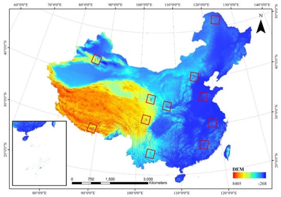
Figure 1.
The study area location with DEM of China (the red box is the study area we used which contains different terrain conditions and the number in the red box represents the number of scenes).
Table 2.
Terrain parameter statistics of Landsat data selected in the study area.
3.2. Data
Landsat 8 surface reflectance products provided an estimate of the surface spectral reflectance as it would be measured at ground level in the absence of atmospheric scattering or absorption [62]. They were generated at the Earth Resources Observation and Science (EROS) Center at a 30-m spatial resolution in the Universal Transverse Mercator Grid System (UTM). Landsat 8 surface reflectance products were obtained from the United States Geological Survey (USGS, https://earthexplorer.usgs.gov/, accessed on 12 October 2021). Cloudless images (cloud cover lower than 10%) acquired in different seasons (January, May, July, September, and November) were selected in each experimental area. Table 3 shows the image acquisition time, solar zenith angle, and snow cover percentage in each image (the snow cover percentage was calculated by the land type stratification described in Section 2.1 in areas with slope angle larger than 5°).
Table 3.
Data acquisition and snow-cover information of Landsat 8 surface reflectance products included for topographic correction evaluation.
In this study, SRTM DEM V003 (the first freely available high resolution DEM [63], obtained from https://search.earthdata.nasa.gov/, accessed on 12 October 2021) with a 1 arc-second resolution (~30 m) in WGS84 was used to calculate slope, aspect, and cast shadows.
3.3. Data Processing
Some necessary processing steps were completed before the implementation of topographic correction methods. After the SRTM DEM data were mosaicked in the study area, they were reprojected onto the same zone of UTM coordinate system as the corresponding Landsat 8 image. Cubic resampling and clipping were applied to DEM data so that they could be matched with the Landsat 8 data in the spatial domain. Aspect and slope parameters were then calculated from the DEM data. The mean solar azimuth/zenith angles were used, and sensor viewing angles were calculated pixel-by-pixel based on the location and acquisition time. Cast shadow and cloud areas can influence the effect of some algorithms and prejudice the evaluation results, thus they were detected in the preprocessing step. The cast shadow was detected by subtracting the self-shadow from the full shadow area [64], and the full shadow detection method was based on the geometric relationship between sunlight direction and mountains, and can refer to Li, Toshio, and Cheng [56]. Cloud detection was adopted by Fmask 4.0 [65], and both cloud and cloud-shadow pixels were eliminated before correction. However, snow is easily confused with clouds, thus we did not adopt Fmask in winter images to avoid hidden problems, and cloud cover in these images is small and can be ignored. Figure 2 is the flow chart of data processing for topographic correction in this study.
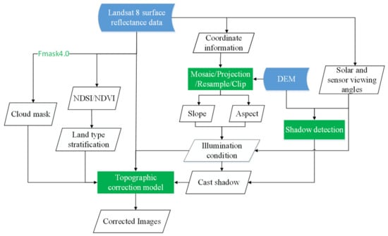
Figure 2.
Flow chart of data processing for Landsat topographic correction.
4. Results
4.1. Outlier Analysis
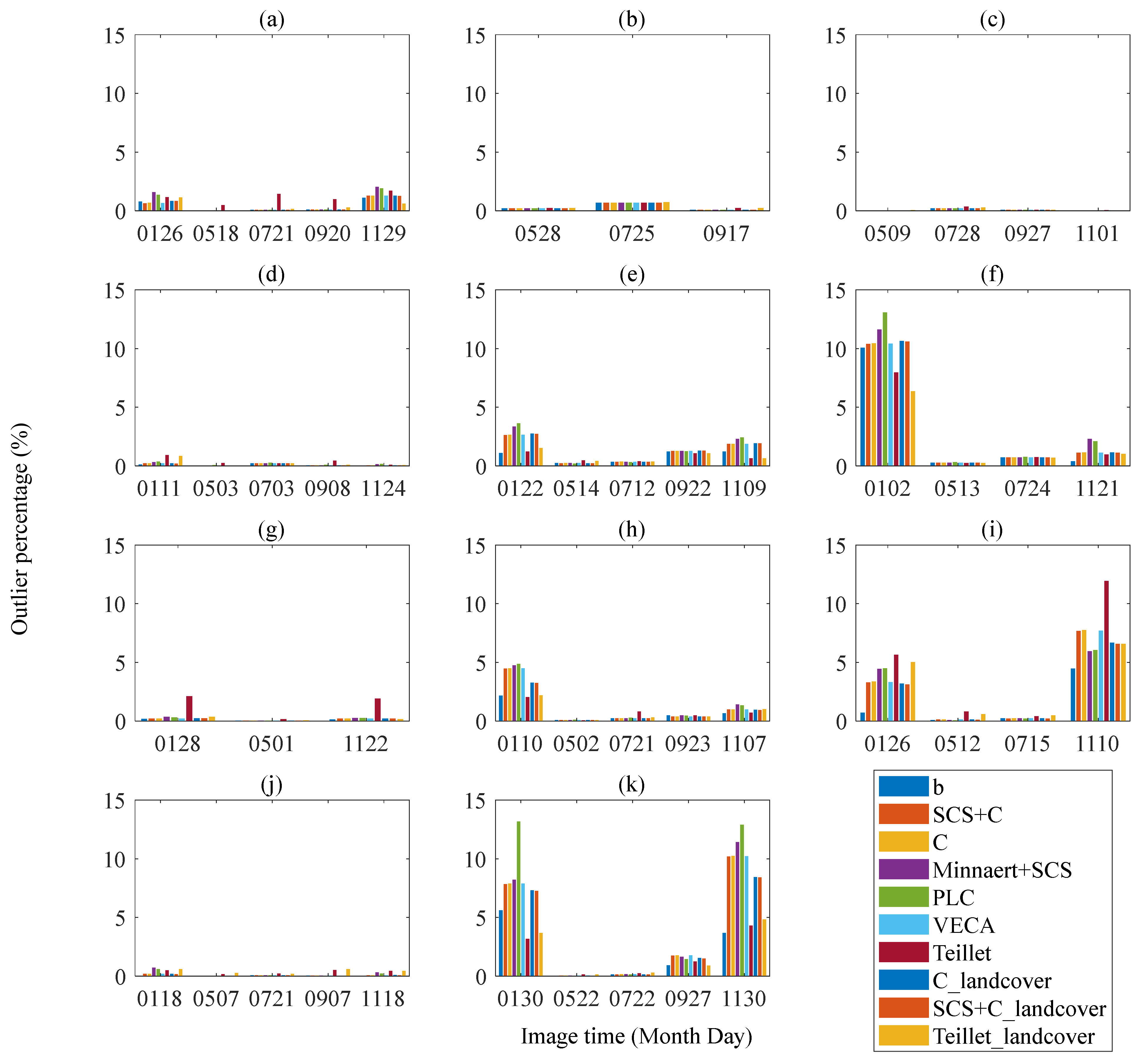
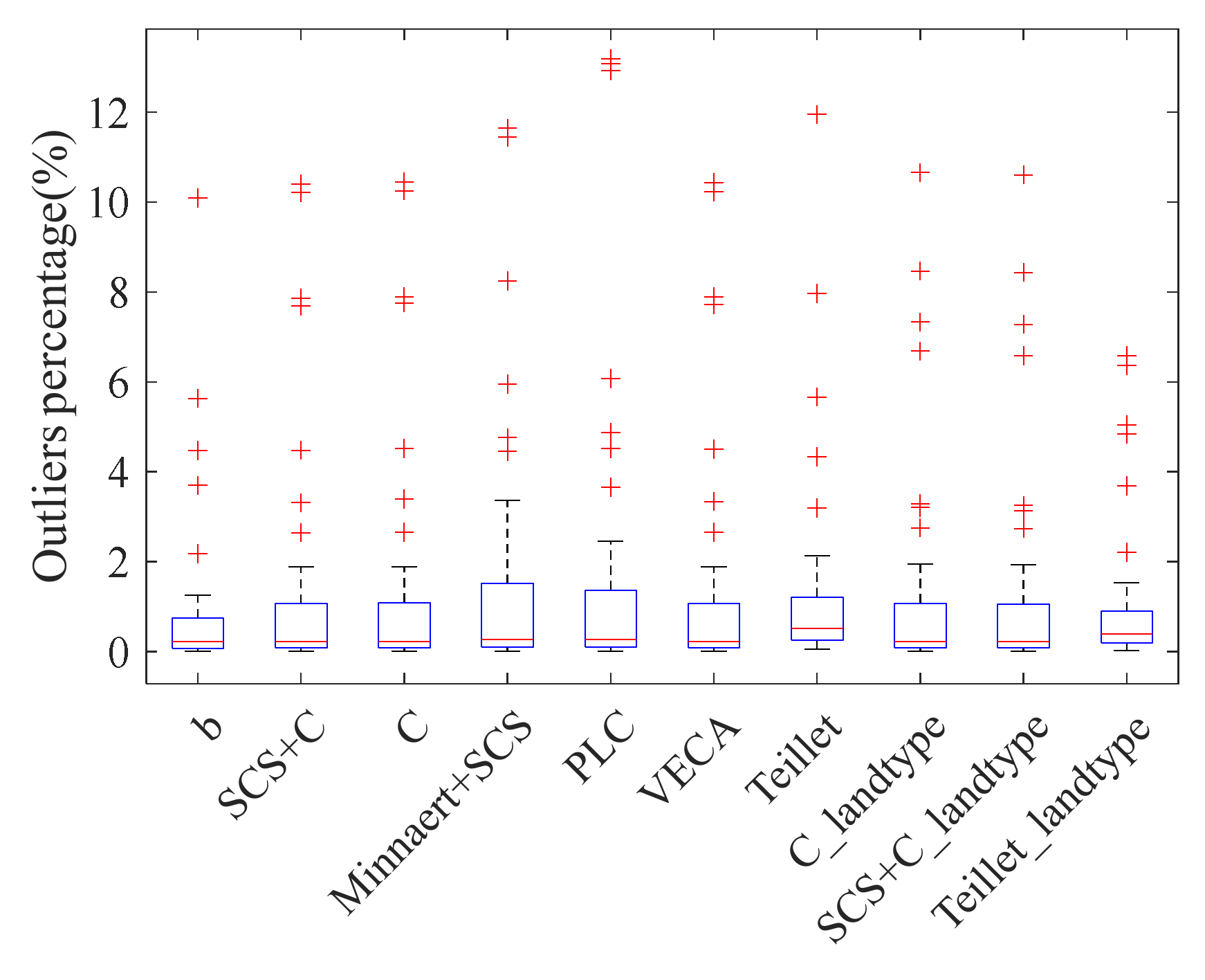
The number of outliers is the primary assessment method as good topographic correction methods should maintain a spatially continuous correction of surface and not produce many outliers. It should be noted that outlier calculation included cast shadow areas to find out each model’s overall performance in mountainous areas. Figure 3 shows the outlier percentage in each Landsat footprint with different time. The box plots of each topographic correction model’s outlier percentage on all images are shown in Figure 4.

Figure 3.
The outlier percentage in different Landsat footprint with different time. (a) path/row:120/039, (b) path/row: 121/024, (c) path/row: 121/042, (d) path/row:122/035, (e) path/row:124/032, (f) path/row: 128/036, (g) path/row:129/043, (h) path/row:131/035, (i) path/row: 131/038, (j) path/row: 139/040, (k) path/row: 143/030.
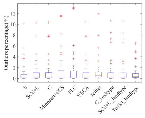
Figure 4.
The box plot of all topographic correction models’ outlier percentages (‘_landtype’ refers to the results using the land type stratification method).
From Figure 3 and Figure 4, these algorithms always offered similar outlier percentages in the same image in May/July/September, and outliers were produced mainly in winter. The Minnaert+SCS and PLC model led to the largest numbers of outliers. The b correction, SCS+C, VECA, and C models offers a lower number of outliers compared with the Teillet regression model. The land type stratification decreased the outliers of the Teillet regression model effectively, and the effect of land type stratification was not obvious for C and SCS+C model. The outlier percentage also showed large differences even in winter, e.g., the outlier percentage of January was larger than November’s in Figure 3f,h, but the reverse was the case in Figure 3i.
4.2. Difference in Sunlit and Shadow Areas
A comparison of the difference in sunlit and shady areas was carried out for different algorithms in all spectral bands to determine which gave the best result, and to check whether slight overcorrection was produced. The relationship between median reflectance in sunlit and shady areas for each model was shown in Figure 5.
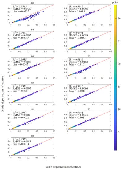
Figure 5.
The relationship of median reflectance in sunlit and shady areas for each model using seven spectral band (sample size = 203). (a) Original image, (b) b correction, (c) SCS+C model, (d) C model, (e) Minnaert+SCS, (f) PLC, (g) VECA, (h) Teillet regression, (i) C with land type stratification, (j) SCS+C with land type stratification, (k) Teillet regression with land type stratification.
From Figure 5, the uncorrected images have a large difference between sunlit and shady slope’s median reflectance, and all topographic correction algorithms provide reduction of the difference. The b correction and Minnaert+SCS model had positive bias value, which indicated that the shady area’s reflectance exceeded the sunlit area’s reflectance after correction, which may be caused by an overcorrection problem. The PLC model resulted in larger sunlit and shady areas’ difference than other models. The Teillet regression model outperformed other non-stratification algorithms with lower RMSE and smaller negative bias. Models with land type stratification can achieve better result than the original models.
4.3. IQR Analysis
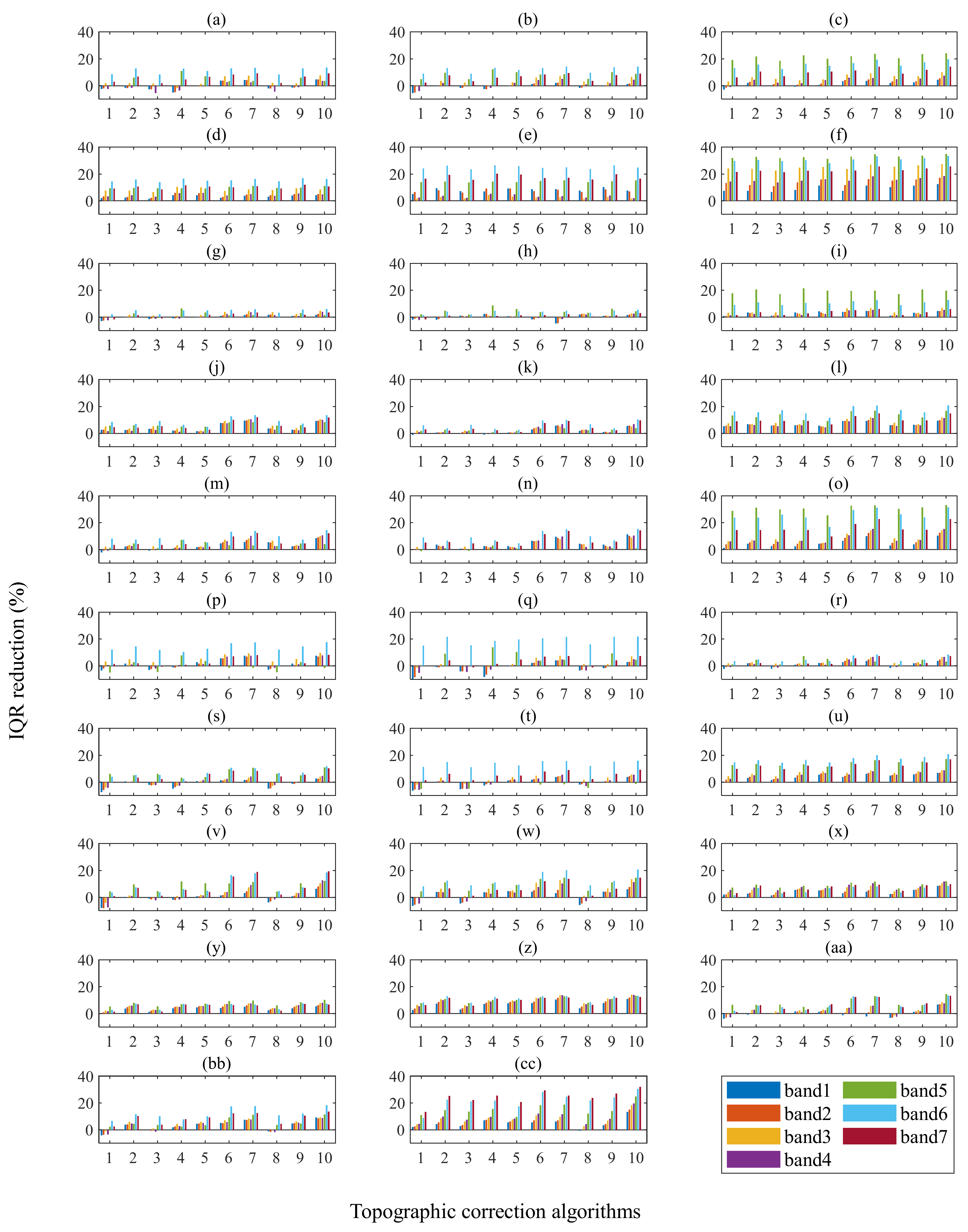
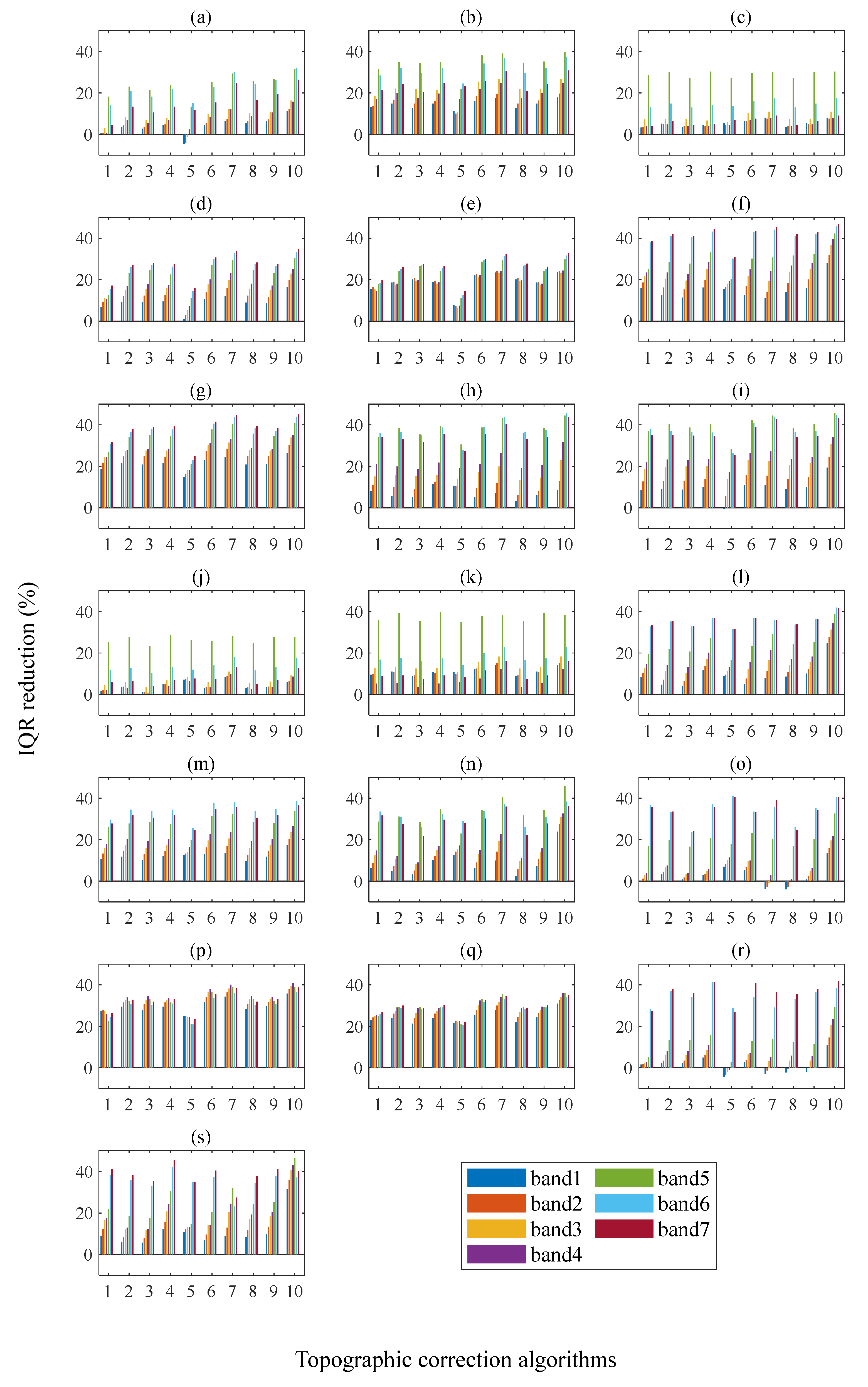
IQR reduction shows the effect of topographic effects’ removal, and a comparison of different algorithms’ IQR reduction in May/July/September and January/November is shown in Figure 6 and Figure 7, respectively.
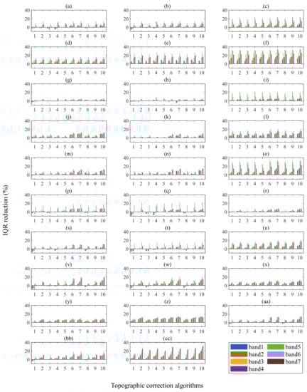
Figure 6.
The comparison of IQR reduction in May/July/September. The x label’s number represents different algorithms: b correction, SCS+C, C, Minnaert+SCS, PLC, VECA, Teillet regression, C with land type stratification, SCS+C with land type stratification, and Teillet regression with land type stratification. (a) 120,039 (path/row) image obtained on 20170518, (b) 120,039 image obtained on 20170721, (c) 120,039 image obtained on 20160920, (d) 121,024 image obtained on 20180528, (e) 121,024 image obtained on 20160725, (f) 121,024 image obtained on 20180917, (g) 121,042 image obtained on 20170509, (h) 121,042 image obtained on 20170728, (i) 121,042 image obtained on 20160927, (j) 122,035 image obtained on 20180503, (k) 122,035 image obtained on 20170703, (l) 122,035 image obtained on 20180908, (m) 124,032 image obtained on 20170514, (n) 124,032 image obtained on 20170712, (o) 124,032 image obtained on 20180922, (p) 128,036 image obtained on 20180513, (q) 128,036 image obtained on 20150724, (r) 129,043 image obtained on 20170501, (s) 131,035 image obtained on 20180502, (t) 131,035 image obtained on 20180721, (u) 131,035 image obtained on 20180923, (v) 131,038 image obtained on 20160512, (w) 131,038 image obtained on 20160715, (x) 139,040 image obtained on 20170507, (y) 139,040 image obtained on 20150721, (z) 139,040 image obtained on 20150907, (aa) 143,030 image obtained on 20180522, (bb) 143,030 image obtained on 20170722, (cc) 143,030 image obtained on 20180927.
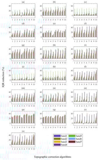
Figure 7.
The comparison of IQR reduction in January/November. The x label number represents different algorithms: b correction, SCS+C, C, Minnaert+SCS, PLC, VECA, Teillet regression, C with land type stratification, SCS+C with land type stratification, and Teillet regression with land type stratification. (a) 120,039 (path/row) image obtained on 20170126, (b) 120,039 image obtained on 20181129, (c) 121,042 image obtained on 20171101, (d) 122,035 image obtained on 20180111, (e) 122,035 image obtained on 20171124, (f) 124,032 image obtained on 20170122, (g) 124,032 image obtained on 20181109, (h) 128,036 image obtained on 20170102, (i) 128,036 image obtained on 20181121, (j) 129,043 image obtained on 20180128, (k) 129,043 image obtained on 20161122, (l) 131,035 image obtained on 20180110, (m) 131,035 image obtained on 20171107, (n) 131,038 image obtained on 20180126, (o) 131,038 image obtained on 20,181,110 (p) 139,040 image obtained on 20180118, (q) 139,040 image obtained on 20181118, (r) 143,030 image obtained on 20180130, (s) 143,030 image obtained on 20181130.
From Figure 6 and Figure 7, it was obvious that the removal of topographic effects in winter was much higher, which was caused by high Sun zenith angle and thus more topographic effects in winter. In contrast, topographic effects were less significant in May/July/September, and thus the effectiveness of algorithms was not obvious, which resulted in low IQR reduction. Meanwhile, different models had similar IQR reduction distribution for different spectral bands in the same image, which indicated the relative coincident of different algorithms and topographic effects depended on spectral bands.
Negative IQR reduction did not correspond with the object of the topographic normalization, however, it occurred in some images, such as Figure 6a,p,q,t. This phenomenon happened mainly for b correction, C model with or without land type stratification. The Teillet regression model produced higher IQR reduction in most images; while PLC had a slightly lower IQR reduction than others in Figure 7, but similar or even larger IQR reduction in Figure 6. In Figure 7o,r, the IQR reduction in all algorithms was not satisfactory; in this image, most algorithms produced small or even negative IQR reduction except the Teillet regression model with land type stratification; in the same scene both in winter (Figure 7n,s), however, most algorithms offered much better performance. Land type stratification improved Teillet regression significantly, while the improvements for C and SCS+C model were not evident.
4.4. Evaluation with LESS Simulation
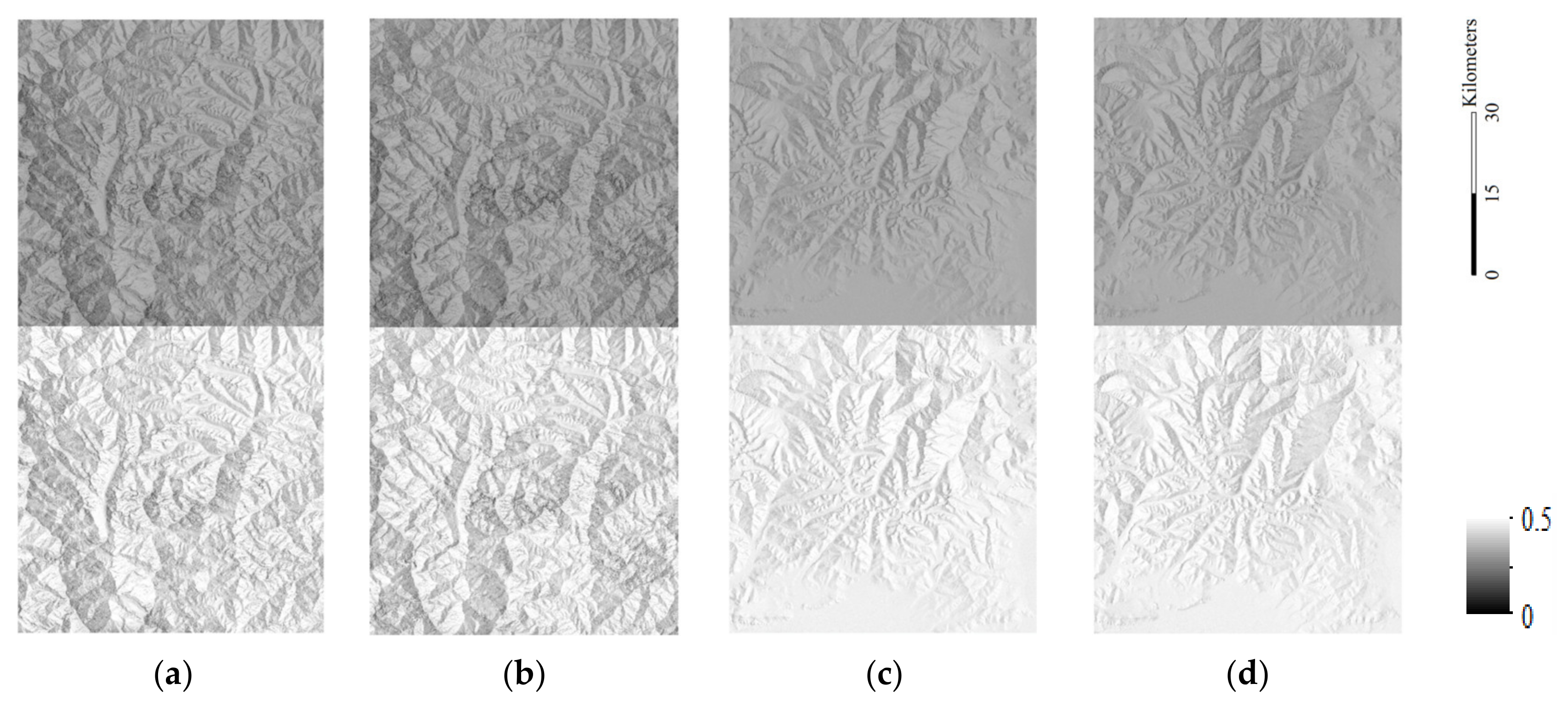
In LESS simulation, images with different terrain conditions were generated to explore the performance of topographic correction methods. Two scenes with two solar azimuth angles (90° and 270° respectively) were simulated, the scene was created by repeating the same DEM but was simulated with soil and vegetation spectral reflectance to figure out the effect of algorithms in images with different land types. Figure 8 shows the simulation result in the NIR band (0.85–0.88 μm).
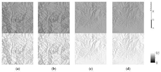
Figure 8.
The LESS simulation results in two scenes with 30° and 270° solar azimuth angle (SAA). They are in NIR band, in 30 m resolution with 3800 × 1900 pixels. The upper area has soil reflectance property (lower reflectance), while the nether area has leaf reflectance property (higher reflectance). (a) is scene 1 with 90° SAA; (b) is scene 1 with 270° SAA; (c) is the scene 2 with 90° SAA; (d) is scene 2 with 270° SAA.
By adopting nine topographic correction methods, the images after correction all showed different levels of elimination of topographic effects. The PLC model was not adopted, because the “orthographic” sensor type was simulated in LESS, and thus unfeasible for the basis of the algorithm.
The evaluation methods for topographic correction algorithms here included IQR reduction, RMSE, and bias compared with plane images, and mean reflectance was also calculated for in-depth understanding of these algorithms. The validation parameters of topographic correction methods in different images are listed in Table 4.
Table 4.
The comparison of topographic correction methods in different simulated images.
Consistent with the former sections, the Minnaert+SCS did not show good performance with highest RMSE, largest bias, and smallest IQR reduction. Meanwhile, SCS+C did not offer good results in this evaluation mainly due to the simulation limitations: we cannot simulate enough trees in such large scenes, but the SCS+C model was put forward to solve the STS model’s problem in forest areas. Our evaluation here also indicated better performance of the C model than the SCS+C model in bare land areas. The C model and b correction model offered better results, which had low RMSE, low bias, and relatively high IQR reduction.
The VECA and Teillet regression model both produced high IQR reduction, but large bias and high RMSE. The mean reflectance of the simulated plane images was 0.407, and bias was found to be related to the mean reflectance value of the uncorrected images, for example, the bias can reach to −0.045 in scene 1, and the mean reflectance value of uncorrected is 0.3619, which had about −0.045 deviation compared with the mean reflectance of plane image. Similar findings were also identified in scene 2. Land type stratification improved the Teillet regression model’s IQR reduction, but there was little improvement in the reduction of bias. There was no obvious improvement for the SCS+C and C model when adopting land type stratification. The RMSE of different algorithms varied in different scenes; since these algorithms always have empirical parameters, the performance of them depend largely on the empirical parameters’ calculation.
5. Discussion
In this work, we focused on topographic correction models’ evaluation and intercomparison. Based on a large number of images with different terrain conditions and seasons, the in-depth analysis for topographic correction algorithms was carried out using a combination of different evaluation methods. LESS simulation helped us discover some problems and drawbacks of algorithms which have not been mentioned before.
5.1. Analysis of Evaluation Results
By analyzing the outliers introduced by different algorithms, we could find which algorithms produced many outliers and invalid data. More outliers appeared in winter, which can be explained by deep terrain effects causing various problems for different topographic correction methods. For example, these images with deep terrain effects not only had self-shadow, but also had considerable cast shadow, which caused deviations for corrected images [64]. Many invalid values in Minnaert+SCS were generated because of the exponential form in these algorithms: the area with negative illumination condition would result in invalid pixels. The PLC model also produced more outliers than other algorithms, especially in winter times, which is caused by the limitation of path length computation in rugged terrains, and thus the PLC model may not be a good choice for steep terrain areas or images with a large solar zenith angle. The number of outliers in C, SCS+C, and VECA was lower than in the Teillet regression model, and the reason is that algorithms with ratio format can introduce some invalid values when the denominator is close to 0, but they are beneficial for scope limitations, while the Teillet regression model may produce more outliers slightly exceeding the original range once coefficients are not ideal. Therefore, the land type stratification significantly reduced the outliers produced by the Teillet regression model, but the effect for the C and SCS+C models was not evident.
The difference between sunlit and shady areas showed the effect of topographic effects’ removal. However, the images for this evaluation should be carefully selected, because when terrain orientations determined the surface properties or land type (e.g., sunlit area covered by bare land, and shady area covered by snow), this evaluation would introduce problems in comparison and analysis. Therefore, we only focused on the overall results, not specific images. The results showed the overcorrection in b correction and Minnaert+SCS models, and land type stratification improved C, SCS+C, and Teillet regression models greatly.
The IQR reductions were higher in winter owing to larger topographic effects, but it also showed large differences in the same footprint in January and November (Figure 7). We concluded that the different land type resulted in this problem (snow-cover can influence the model’s parameters calculation largely without land type stratification), and the results were largely improved by adopting land type stratification for the Teillet regression model.
Many evaluation studies compared the correlation coefficients between reflectance and illumination angles [6,37,38,39]. However, the result may not be valid where slope orientation determines land cover or vegetation growth status [10]. Furthermore, the relation between reflectance and illumination angle has been incorporated into some topographic correction models, such as the VECA model and the Teillet regression model, and using the correlation coefficients again as the evaluation method may not be impartial.
The validation using LESS simulation is an effective way to avoid some assumptions in the evaluation and can explore the bias between corrected images and “true values”. The evaluation results by LESS simulation confirm the former comparison, and the C model performed best in the evaluation with smallest RMSE and least bias (this result was based on unforested simulations), and it corresponded with the former studies based on synthetic images [34,41]. In our study, correction bias was concentrated for further analysis based on LESS simulations for the first time. The bias was found in Teillet regression model and VECA when the original images had large bias with the simulated plane image and could be explained by the utilization of mean reflectance in the algorithm, assuming that the mean reflectance of the image is close to the “true value”. However, the bias would be introduced into the corrected image when the mean reflectance had large bias from the “true value”; and the C model also showed slight bias changing with scenes. Based on this, the mean value was not recommended for stability evaluation for topographic correction models [38], because the utilization of mean reflectance in some algorithms (Teillet regression model and VECA) would show partiality in the comparison. Although large bias also appeared in SCS+C model, the IQR reduction was not that high and could be caused by the improper correction of SCS strategy for unforested areas. Due to the utilization of empirical parameters in these algorithms, the performance of them was closely related to the parameters’ calculation and the complexity of the surface ground. It should be noted that the evaluation based on simulation image in our study can offer more information about different algorithms, but we did not totally depend on it owing to more complex situations in remote sensing images.
5.2. Summary of Different Topographic Correction Algorithms
Different evaluation indicators aim to assess different aspects of topographic correction models, so it is necessary to combine these assessment methods to carry out a more systematic comparison [34,42]. By using different methods to validate algorithms, they showed diverse applicability in varied conditions. The Teillet regression with land type stratification offered good results but may produce bias in some conditions, which is ignored in previous studies [34]. One feasible way for bias decrease and model improvement is to build a high-quality database for parameter fitting [32] instead of training in each image, which would be beneficial for obtaining high-consistency topographic correction data. Meanwhile, in high cloud-cover images, using coefficients from a pre-constructed database is an effective way to provide good estimates.
Owing to the logarithm in the fitting, the negative pixels were removed while calculating in Minnaert+SCS model; the impossibility of making a considerate description about the ground information obstructs the further advancement of the algorithm. The method of calculating path length in steep terrain areas restricted the application of the PLC model, and the topographic mask should be generated before correction [57]. Meanwhile, our study focused on Landsat 8 which has a small view zenith angle, and Yin et al. [21] reported a better performance of the PLC model when the view zenith angle is large. Without depending on empirical parameters, the PLC model may offer higher quality correction results for a time series study. The C model and SCS+C model provided similar performance in outliers and difference between sunlit and shady areas, but the C model offered better results based on LESS simulation (owing to the bare land simulations). Hurni et al. [42] found that the Teillet regression model offered the best performance in most images, but other algorithms can also outperform it in some conditions, which corresponded with our results, and the land type stratification improved Teillet regression model significantly in our study. It verified that the Teillet regression model was sensitive to fitting coefficients and may lead to bad results when the fitting is not ideal, e.g., insufficient fitting pixels or cloud and cast shadow pixels are not totally removed. The algorithms with ratio format (SCS+C and C model) would be less sensitive to land type stratification than the Teillet regression model, because the C parameter is both in the numerator and the denominator, which can lessen the influence of coefficients in different land types. However, the ratio format also introduced errors, such as obvious outliers in the image when the denominator was close to zero.
Land type stratification was found to improve the semi-empirical models, especially for the Teillet regression model in this study, which is inconsistent with [66]. The main reason is that the large surface reflectance difference between snow-free and snow-cover areas can significantly influence the fitting efficiency in some algorithms, and land type stratification markedly improves the images with high snow-cover (Figure 7). However, the snow-cover areas were always ignored in previous research [10,66]. Thus, the conclusion may be conflicting when focused only on a few images with similar land types. Therefore, it is difficult to thoroughly evaluate algorithms in just a small number of images due to complicated conditions in mountainous areas, and we highly recommended evaluating topographic correction methods under different terrain conditions and seasons.
Using a computer with i7-9750H CPU and 16 GB memory for this experiment, the Teillet regression model took 103 s for each Landsat 8 image, and it was 174 s for the Teillet regression with land type stratification, which is acceptable for research and application. Other topographic correction methods without land type stratification used a similar amount of time as the Teillet regression model did, while the PLC was the most time efficient of them all.
5.3. Limitations and Applications
Problems also existed with these algorithms, such as the neglection of cast shadow, which would introduce some errors while correcting, especially in steep terrain areas. Therefore, relevant modifications should be made on the model [64]. A simple land type stratification strategy was used in this study, and it can be improved or replaced by finer land classification product in the future. The 3D radiative transfer model is time and memory consuming, and the simulation of a large number of trees in the scene is limited, which makes it difficult to evaluate the algorithms’ performance in forest areas.
Owing to the above issues in topographic correction algorithms, we here discuss the precautions that need to be taken when using topographic correction. Some studies have utilized topographic correction methods for land cover and vegetation classification, and reached good results in mountains [6,7,35,67]. Since the classification relied more on the difference of different land types and was not very sensitive to the absolute value of the image, topographic correction methods can eliminate the difference of the same land cover pixels in different terrain conditions; thus, it is helpful to apply topographic correction for image classification.
However, when it comes to surface parameters retrieval, the bias caused by topographic correction algorithms may exceed the errors in the estimation method itself (e.g., large RMSE in scene for some algorithms in Table 4). It was also proven that the utilization of sloping reflectance directly offered better results than the reflectance after topographic correction for estimation of albedo [68]. Thus, we recommend users consider the pros and cons before using a topographic correction algorithm for surface parameter retrieval, especially for parameters related to radiation, such as surface albedo estimation [69], and net radiation [70]; and the further developing estimation algorithms for surface parameters on sloping terrains should couple with the topography rather than apply topographic corrections [68,71].
6. Conclusions
This study validated the effect of different topographic correction methods in large areas and different seasons. The advantages and disadvantages in different topographic correction methods are obvious after comparing a large number of images. Most algorithms provided worse results in snow-cover areas, while land type stratification could improve the Teillet regression model. The Teillet regression model, which was most recommended in previous studies, showed bias in the evaluation using simulated images.
The validation results showed large differences even in the same Landsat footprint in January and November, and the land type stratification can markedly decrease this difference for the Teillet regression model. It also indicated the necessity of evaluation based on a large number of images.
LESS simulation offers an effective way to assess the correction bias, and large bias was found in the Teillet and VECA model when there was bias between the mean reflectance value in uncorrected images and the “true reflectance”. We recommend the implementation of simulation images to evaluate the topographic correction models, which can facilitate in-depth analysis.
Owing to the issues in different algorithms and complicated conditions in rugged terrain, we recommended taking into account the pros and cons of topographic correction methods for surface parameter retrieval in mountain regions and integrating topographic considerations into mountainous retrieval methods directly rather than adopting topographic correction before retrieval.
Author Contributions
Conceptualization, T.H.; methodology and experiments, Y.M.; writing—original draft preparation, Y.M.; writing—review and editing, T.H., A.L. and S.L. All authors have read and agreed to the published version of the manuscript.
Funding
This research was funded by National Key Research and Development Program of China (2020YFA0608704), National Natural Science Foundation of China Grant (42090012) and in part by the Innovative Research Groups of the Hubei Natural Science under Grant 2020CFA003. We gratefully acknowledge data support from the National Earth System Science Data Center, National Science & Technology Infrastructure of China (http://www.geodata.cn, accessed on 18 September 2021).
Acknowledgments
The authors acknowledge the United States Geological Survey and NASA Earth Science Data Systems for the provision of the Landsat surface reflectance product and SRTM DEM. We extend our thanks to Jianbo Qi and Jiang Chen for helping us complete LESS simulation and draw figures, respectively. We are also grateful to Minfeng Xing’s comments in the early stage of our work.
Conflicts of Interest
The authors declare no conflict of interest.
References
- Blyth, S.; Lysenko, I.; Groombridge, B.; Miles, L.; Newton, A. Mountain Watch: Environmental Change and Sustainable Development in Mountains; UNEP-WCMC: Cambridge, UK, 2002. [Google Scholar]
- Bian, J.; Li, A.; Lei, G.; Zhang, Z.; Nan, X. Global high-resolution mountain green cover index mapping based on Landsat images and Google Earth Engine. ISPRS J. Photogramm. Remote Sens. 2020, 162, 63–76. [Google Scholar] [CrossRef]
- Immerzeel, W.W.; Lutz, A.F.; Andrade, M.; Bahl, A.; Biemans, H.; Bolch, T.; Hyde, S.; Brumby, S.; Davies, B.J.; Elmore, A.C.; et al. Importance and vulnerability of the world’s water towers. Nature 2020, 577, 364–369. [Google Scholar] [CrossRef]
- Meyer, P.; Itten, K.I.; Kellenberger, T.; Sandmeier, S.; Sandmeier, R. Radiometric corrections of topographically induced effects on Landsat TM data in an alpine environment. ISPRS J. Photogramm. Remote Sens. 1993, 48, 17–28. [Google Scholar] [CrossRef]
- Jin, H.; Li, A.; Xu, W.; Xiao, Z.; Jiang, J.; Xue, H. Evaluation of topographic effects on multiscale leaf area index estimation using remotely sensed observations from multiple sensors. ISPRS J. Photogramm. Remote Sens. 2019, 154, 176–188. [Google Scholar] [CrossRef]
- Moreira, E.P.; Valeriano, M.M. Application and evaluation of topographic correction methods to improve land cover mapping using object-based classification. Int. J. Appl. Earth Obs. Geoinf. 2014, 32, 208–217. [Google Scholar] [CrossRef]
- Phiri, D.; Morgenroth, J.; Xu, C.; Hermosilla, T. Effects of pre-processing methods on Landsat OLI-8 land cover classification using OBIA and random forests classifier. Int. J. Appl. Earth Obs. Geoinf. 2018, 73, 170–178. [Google Scholar] [CrossRef]
- Cuo, L.; Vogler, J.B.; Fox, J.M. Topographic normalization for improving vegetation classification in a mountainous watershed in Northern Thailand. Int. J. Remote Sens. 2010, 31, 3037–3050. [Google Scholar] [CrossRef]
- Yu, W.; Li, J.; Liu, Q.; Yin, G.; Zeng, Y.; Lin, S.; Zhao, J. A Simulation-Based Analysis of Topographic Effects on LAI Inversion Over Sloped Terrain. IEEE J. Sel. Top. Appl. Earth Obs. Remote Sens. 2020, 13, 794–806. [Google Scholar] [CrossRef]
- Hantson, S.; Chuvieco, E. Evaluation of different topographic correction methods for Landsat imagery. Int. J. Appl. Earth Obs. Geoinf. 2011, 13, 691–700. [Google Scholar] [CrossRef]
- Wu, Q.; Jin, Y.; Fan, H. Evaluating and comparing performances of topographic correction methods based on multi-source DEMs and Landsat-8 OLI data. Int. J. Remote Sens. 2016, 37, 4712–4730. [Google Scholar] [CrossRef]
- Zhang, W.; Gao, Y. Topographic correction algorithm for remotely sensed data accounting for indirect irradiance. Int. J. Remote Sens. 2011, 32, 1807–1824. [Google Scholar] [CrossRef]
- Wen, J.; Liu, Q.; Liu, Q.; Xiao, Q.; Li, X. Parametrized BRDF for atmospheric and topographic correction and albedo estimation in Jiangxi rugged terrain, China. Int. J. Remote Sens. 2009, 30, 2875–2896. [Google Scholar] [CrossRef]
- Balthazar, V.; Vanacker, V.; Lambin, E.F. Evaluation and parameterization of ATCOR3 topographic correction method for forest cover mapping in mountain areas. Int. J. Appl. Earth Obs. Geoinf. 2012, 18, 436–450. [Google Scholar] [CrossRef]
- Blesius, L.; Weirich, F. The use of the Minnaert correction for land-cover classification in mountainous terrain. Int. J. Remote Sens. 2005, 26, 3831–3851. [Google Scholar] [CrossRef]
- Sandmeier, S.; Itten, K.I. A physically-based model to correct atmospheric and illumination effects in optical satellite data of rugged terrain. IEEE Trans. Geosci. Remote Sens. 1997, 35, 708–717. [Google Scholar] [CrossRef] [Green Version]
- Zhao, W.; Li, X.; Wang, W.; Wen, F.; Yin, G. DSRC: An Improved Topographic Correction Method for Optical Remote-Sensing Observations Based on Surface Downwelling Shortwave Radiation. IEEE Trans. Geosci. Remote Sens. 2021, 1–15. [Google Scholar] [CrossRef]
- Soenen, S.A.; Peddle, D.R.; Coburn, C.A.; Hall, R.J.; Hall, F.G. Improved topographic correction of forest image data using a 3-D canopy reflectance model in multiple forward mode. Int. J. Remote Sens. 2008, 29, 1007–1027. [Google Scholar] [CrossRef]
- Li, X.; Strahler, A.H. Geometric-optical bidirectional reflectance modeling of the discrete crown vegetation canopy: Effect of crown shape and mutual shadowing. IEEE Trans. Geosci. Remote Sens. 1992, 30, 276–292. [Google Scholar] [CrossRef]
- Li, F.; Jupp, D.L.B.; Thankappan, M.; Lymburner, L.; Mueller, N.; Lewis, A.; Held, A. A physics-based atmospheric and BRDF correction for Landsat data over mountainous terrain. Remote Sens. Environ. 2012, 124, 756–770. [Google Scholar] [CrossRef]
- Yin, G.; Li, A.; Wu, S.; Fan, W.; Zeng, Y.; Yan, K.; Xu, B.; Li, J.; Liu, Q. PLC: A simple and semi-physical topographic correction method for vegetation canopies based on path length correction. Remote Sens. Environ. 2018, 215, 184–198. [Google Scholar] [CrossRef]
- Szantoi, Z.; Simonetti, D. Fast and robust topographic correction method for medium resolution satellite imagery using a stratified approach. IEEE J. Sel. Top. Appl. Earth Obs. Remote Sens. 2013, 6, 1921–1933. [Google Scholar] [CrossRef]
- Smith, J.A.; Lin, T.L.; Ranson, K.L. The Lambertian assumption and Landsat data. Photogramm. Eng. Remote Sens. 1980, 46, 1183–1189. [Google Scholar]
- Minnaert, M. The reciprocity principle in lunar photometry. Astrophys. J. 1941, 93, 403–410. [Google Scholar] [CrossRef]
- Teillet, P.; Guindon, B.; Goodenough, D. On the slope-aspect correction of multispectral scanner data. Can. J. Remote Sens. 1982, 8, 84–106. [Google Scholar] [CrossRef] [Green Version]
- Gu, D.; Gillespie, A. Topographic normalization of Landsat TM images of forest based on subpixel Sun–Canopy–Sensor geometry. Remote Sens. Environ. 1998, 64, 166–175. [Google Scholar] [CrossRef]
- Soenen, S.A.; Peddle, D.R.; Coburn, C.A. SCS+C: A modified Sun-canopy-sensor topographic correction in forested terrain. IEEE Trans. Geosci. Remote Sens. 2005, 43, 2148–2159. [Google Scholar] [CrossRef]
- Vincini, M.; Reeder, D.; Frazzi, E. An empirical topographic normalization method for forest TM data. In Proceedings of the IEEE International Geoscience and Remote Sensing Symposium, Toronto, ON, Canada, 24–28 June 2002; Volume 4, pp. 2091–2093. [Google Scholar]
- Gao, Y.; Zhang, W. Variable empirical coefficient algorithm for removal of topographic effects on remotely sensed data from rugged terrain. In Proceedings of the IEEE International Geoscience and Remote Sensing Symposium, Barcelona, Spain, 23–28 July 2007; pp. 4733–4736. [Google Scholar]
- Riano, D.; Chuvieco, E.; Salas, J.; Aguado, I. Assessment of different topographic corrections in Landsat-TM data for mapping vegetation types (2003). IEEE Trans. Geosci. Remote Sens. 2003, 41, 1056–1061. [Google Scholar] [CrossRef] [Green Version]
- Lu, D.S.; Ge, H.L.; He, S.Z.; Xu, A.J.; Zhou, G.M.; Du, H.Q. Pixel-based Minnaert correction method for reducing topographic effects on a Landsat 7 ETM+ image. Photogramm. Eng. Remote Sens. 2008, 74, 1343–1350. [Google Scholar] [CrossRef] [Green Version]
- Reese, H.; Olsson, H. C-correction of optical satellite data over alpine vegetation areas: A comparison of sampling strategies for determining the empirical c-parameter. Remote Sens. Environ. 2011, 115, 1387–1400. [Google Scholar] [CrossRef] [Green Version]
- Vázquez-Jiménez, R.; Romero-Calcerrada, R.; Ramos-Bernal, R.N.; Arrogante-Funes, P.; Novillo, C.J. Topographic correction to Landsat imagery through slope classification by applying the SCS + C method in mountainous forest areas. ISPRS Int. J. Geo-Inf. 2017, 6, 287. [Google Scholar] [CrossRef]
- Sola, I.; Gonzalez-Audicana, M.; Alvarez-Mozos, J. Multi-criteria evaluation of topographic correction methods. Remote Sens. Environ. 2016, 184, 247–262. [Google Scholar] [CrossRef] [Green Version]
- Dong, C.; Zhao, G.; Meng, Y.; Li, B.; Peng, B. The Effect of Topographic Correction on Forest Tree Species Classification Accuracy. Remote Sens. 2020, 12, 787. [Google Scholar] [CrossRef] [Green Version]
- Gao, Y.; Zhang, W. A simple empirical topographic correction method for ETM+ imagery. Int. J. Remote Sens. 2009, 30, 2259–2275. [Google Scholar] [CrossRef]
- Richter, R. Correction of satellite imagery over mountainous terrain. Appl. Opt. 1998, 37, 4004–4015. [Google Scholar] [CrossRef] [PubMed]
- Ghasemi, N.; Mohammadzadeh, A.; Sahebi, M.R. Assessment of different topographic correction methods in ALOS AVNIR-2 data over a forest area. Int. J. Digit. Earth 2013, 6, 504–520. [Google Scholar] [CrossRef]
- Vanonckelen, S.; Lhermitte, S.; Balthazar, V.; Van Rompaey, A. Performance of atmospheric and topographic correction methods on Landsat imagery in mountain areas. Int. J. Remote Sens. 2014, 35, 4952–4972. [Google Scholar] [CrossRef] [Green Version]
- Civco, D.L. Topographic normalization of landsat thematic mapper digital imagery. Photogramm. Eng. Remote Sens. 1989, 55, 1303–1309. [Google Scholar]
- Sola, I.; González-Audícana, M.; Álvarez-Mozos, J.; Torres, J.L. Synthetic Images for Evaluating Topographic Correction Algorithms. IEEE Trans. Geosci. Remote Sens. 2014, 52, 1799–1810. [Google Scholar] [CrossRef]
- Hurni, K.; Van Den Hoek, J.; Fox, J. Assessing the spatial, spectral, and temporal consistency of topographically corrected Landsat time series composites across the mountainous forests of Nepal. Remote Sens. Environ. 2019, 231, 111225. [Google Scholar] [CrossRef]
- Richter, R.; Kellenberger, T.; Kaufmann, H. Comparison of Topographic Correction Methods. Remote Sens. 2009, 1, 184–196. [Google Scholar] [CrossRef] [Green Version]
- Hoshikawa, K.; Umezaki, M. Effects of terrain-induced shade removal using global DEM data sets on land-cover classification. Int. J. Remote Sens. 2014, 35, 1331–1355. [Google Scholar] [CrossRef]
- Gao, M.; Zhao, W.; Gong, Z.; Gong, H.; Chen, Z.; Xin-Ming, T. Topographic correction of ZY-3 satellite images and its effects on estimation of shrub leaf biomass in mountainous areas. Remote Sens. 2014, 6, 2745–2764. [Google Scholar] [CrossRef] [Green Version]
- Qi, J.; Xie, D.; Yin, T.; Yan, G.; Gastellu-Etchegorry, J.-P.; Li, L.; Zhang, W.; Mu, X.; Norford, L.K. LESS: LargE-Scale remote sensing data and image simulation framework over heterogeneous 3D scenes. Remote Sens. Environ. 2019, 221, 695–706. [Google Scholar] [CrossRef]
- Torma, M.; Harma, P. Topographic correction of Landsat ETM-images in finnish lapland. In Proceedings of the IEEE Geoscience and Remote Sensing Symposium, Toulouse, France, 21–25 July 2003. [Google Scholar]
- Bishop, M.P.; Schroder, J.F.; Colby, J.D. Remote sensing and geomorphometry for studying relief production in high mountains. Geomorphology 2003, 55, 345–361. [Google Scholar] [CrossRef] [Green Version]
- Frantz, D.; Röder, A.; Stellmes, M.; Hill, J. An Operational Radiometric Landsat Preprocessing Framework for Large-Area Time Series Applications. IEEE Trans. Geosci. Remote Sens. 2016, 54, 3928–3943. [Google Scholar] [CrossRef]
- Tokola, T.; Sarkeala, J.; Van Der Linden, M. Use of topographic correction in Landsat TM-based forest interpretation in Nepal. Int. J. Remote Sens. 2001, 22, 551–563. [Google Scholar] [CrossRef]
- Zhang, H.; Zhang, F.; Zhang, G.; Che, T.; Yan, W.; Ye, M.; Ma, N. Ground-based evaluation of MODIS snow cover product V6 across China: Implications for the selection of NDSI threshold. Sci. Total Environ. 2019, 651, 2712–2726. [Google Scholar] [CrossRef]
- Qu, Y.; Liu, Q.; Liang, S.; Wang, L.; Liu, N.; Liu, S. Direct-Estimation Algorithm for Mapping Daily Land-Surface Broadband Albedo From MODIS Data. IEEE Trans. Geosci. Remote Sens. 2014, 52, 907–919. [Google Scholar] [CrossRef]
- Burns, P.; Nolin, A. Using atmospherically-corrected Landsat imagery to measure glacier area change in the Cordillera Blanca, Peru from 1987 to 2010. Remote Sens. Environ. 2014, 140, 165–178. [Google Scholar] [CrossRef] [Green Version]
- Riihimäki, H.; Heiskanen, J.; Luoto, M. The effect of topography on arctic-alpine aboveground biomass and NDVI patterns. Int. J. Appl. Earth Obs. Geoinf. 2017, 56, 44–53. [Google Scholar] [CrossRef] [Green Version]
- Henry Reeder, D. Topographic Correction of Satellite Images: Theory and Application; Dartmouth College: Hanover, NH, USA, 2002. [Google Scholar]
- Li, X.; Toshio, K.; Cheng, G. Retrieval of snow reflectance from Landsat data in rugged terrain. Ann. Glaciol. 2002, 34, 31–37. [Google Scholar] [CrossRef] [Green Version]
- Luisa, E.M.; Frederic, B.; Marie, W. Slope correction for LAI estimation from gap fraction measurements. Agric. For. Meteorol. 2008, 148, 1553–1562. [Google Scholar] [CrossRef]
- Vicente-Serrano, S.M.; Pérez-Cabello, F.; Lasanta, T. Assessment of radiometric correction techniques in analyzing vegetation variability and change using time series of Landsat images. Remote Sens. Environ. 2008, 112, 3916–3934. [Google Scholar] [CrossRef]
- Qi, J.; Xie, D.; Guo, D.; Yan, G. A Large-Scale Emulation System for Realistic Three-Dimensional (3-D) Forest Simulation. IEEE J. Sel. Top. Appl. Earth Obs. Remote Sens. 2017, 10, 4834–4843. [Google Scholar] [CrossRef]
- Nan, X.; Li, A.; Yu, C.; Wei, D. Design and compilation of digital mountain map of China (1:6,700,000) in vertical layout. Remote Sens. Technol. Appl. 2016, 31, 451–458. [Google Scholar]
- Zhang, X.; Liu, L.; Chen, X.; Gao, Y.; Xie, S.; Mi, J. GLC_FCS30: Global land-cover product with fine classification system at 30 m using time-series Landsat imagery. Earth Syst. Sci. Data 2021, 13, 2753–2776. [Google Scholar] [CrossRef]
- Vermote, E.; Justice, C.; Claverie, M.; Franch, B. Preliminary analysis of the performance of the Landsat 8/OLI land surface reflectance product. Remote Sens. Environ. 2016, 185, 46–56. [Google Scholar] [CrossRef] [PubMed]
- Carrera-Hernández, J.J. Not all DEMs are equal: An evaluation of six globally available 30 m resolution DEMs with geodetic benchmarks and LiDAR in Mexico. Remote Sens. Environ. 2021, 261, 112474. [Google Scholar] [CrossRef]
- Li, H.; Xu, L.; Shen, H.; Zhang, L. A general variational framework considering cast shadows for the topographic correction of remote sensing imagery. ISPRS J. Photogramm. Remote Sens. 2016, 117, 161–171. [Google Scholar] [CrossRef]
- Qiu, S.; Zhu, Z.; He, B. Fmask 4.0: Improved cloud and cloud shadow detection in Landsats 4–8 and Sentinel-2 imagery. Remote Sens. Environ. 2019, 231, 111205. [Google Scholar] [CrossRef]
- Sola, I.; González-Audícana, M.; Álvarez-Mozos, J. The Added Value of Stratified Topographic Correction of Multispectral Images. Remote Sens. 2016, 8, 131. [Google Scholar] [CrossRef] [Green Version]
- Vanonckelen, S.; Lhermitte, S.; Van Rompaey, A. The effect of atmospheric and topographic correction methods on land cover classification accuracy. Int. J. Appl. Earth Obs. Geoinf. 2013, 24, 9–21. [Google Scholar] [CrossRef] [Green Version]
- Lin, X.; Wu, S.; Hao, D.; Wen, J.; Xiao, Q.; Liu, Q. Sloping Surface Reflectance: The Best Option for Satellite-Based Albedo Retrieval Over Mountainous Areas. IEEE Geosci. Remote Sens. Lett. 2021, 1–5. [Google Scholar] [CrossRef]
- He, T.; Liang, S.; Wang, D.; Cao, Y.; Gao, F.; Yu, Y.; Feng, M. Evaluating land surface albedo estimation from Landsat MSS, TM, ETM+, and OLI data based on the unified direct estimation approach. Remote Sens. Environ. 2018, 204, 181–196. [Google Scholar] [CrossRef]
- He, T.; Liang, S.; Wang, D.; Shi, Q.; Goulden, M.L. Estimation of high-resolution land surface net shortwave radiation from AVIRIS data: Algorithm development and preliminary results. Remote Sens. Environ. 2015, 167, 20–30. [Google Scholar] [CrossRef] [Green Version]
- Zhao, W.; Duan, S.-B.; Li, A.; Yin, G. A practical method for reducing terrain effect on land surface temperature using random forest regression. Remote Sens. Environ. 2019, 221, 635–649. [Google Scholar] [CrossRef]


Publisher’s Note: MDPI stays neutral with regard to jurisdictional claims in published maps and institutional affiliations. |
© 2021 by the authors. Licensee MDPI, Basel, Switzerland. This article is an open access article distributed under the terms and conditions of the Creative Commons Attribution (CC BY) license (https://creativecommons.org/licenses/by/4.0/).