
Extraction of Abandoned Land in Hilly Areas Based on the Spatio-Temporal Fusion of Multi-Source Remote Sensing Images


Abstract
:
1. Introduction
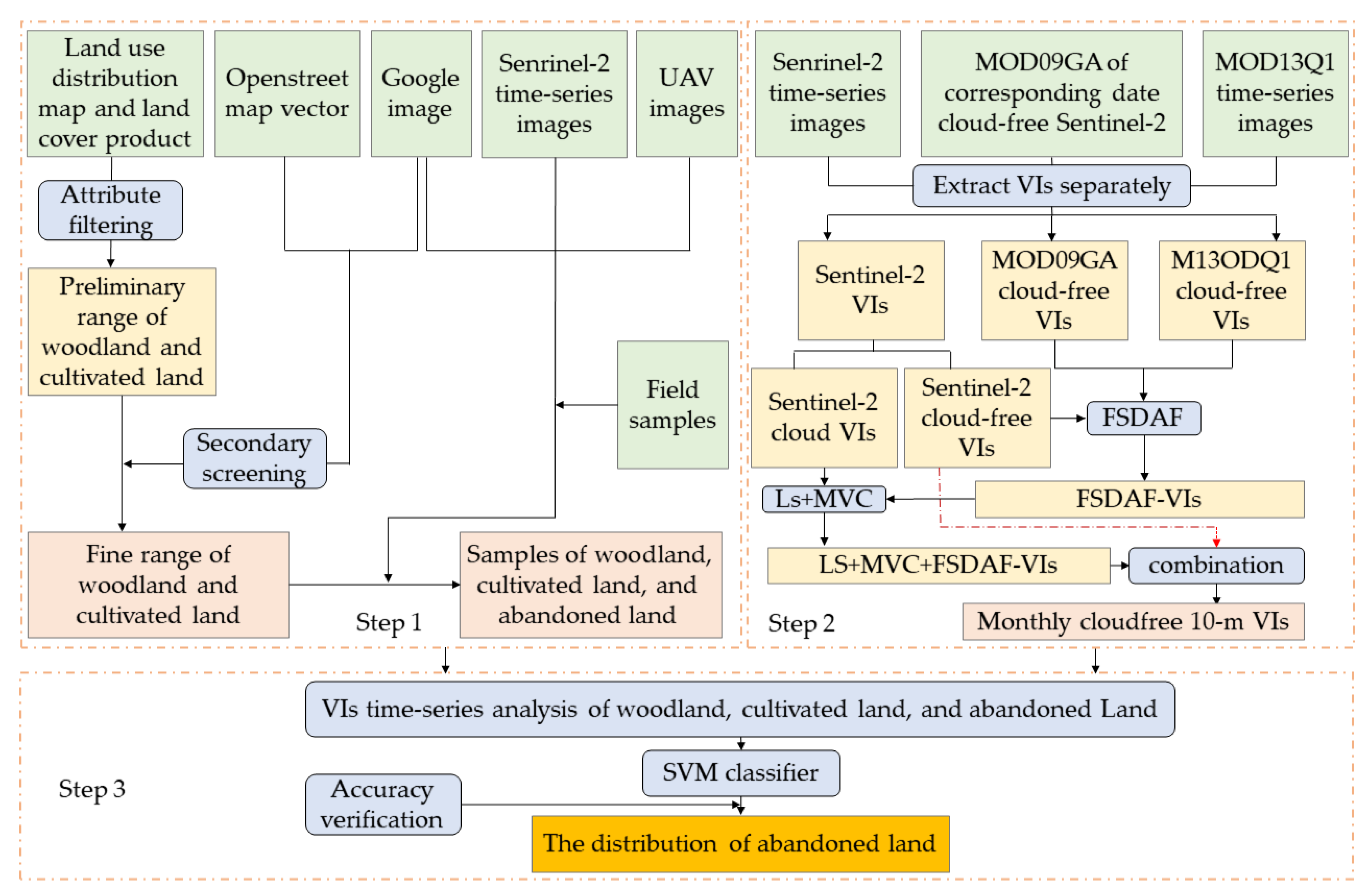
2. Materials and Methods
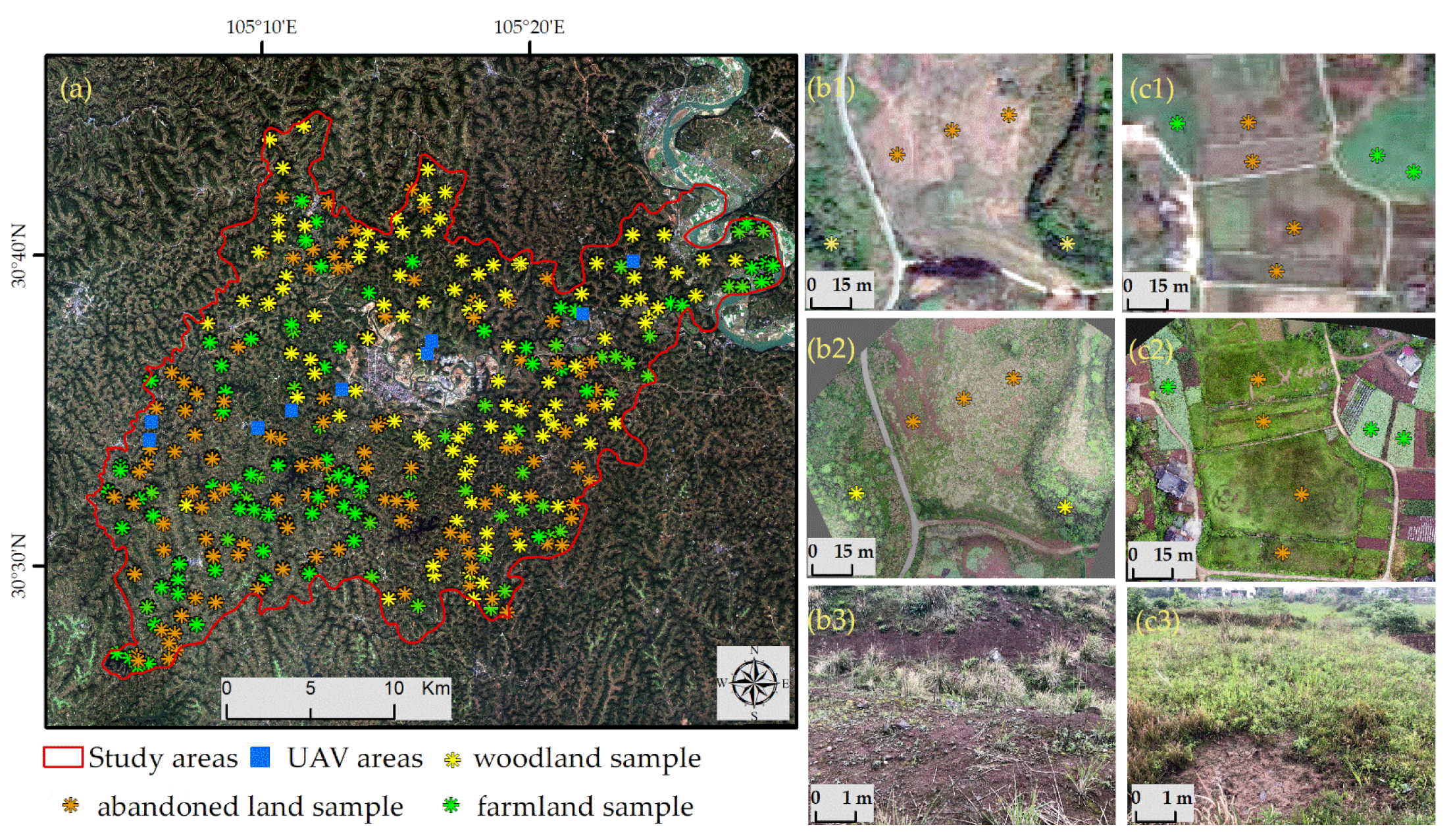
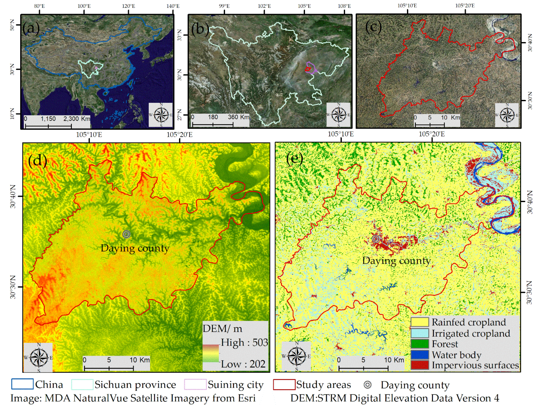
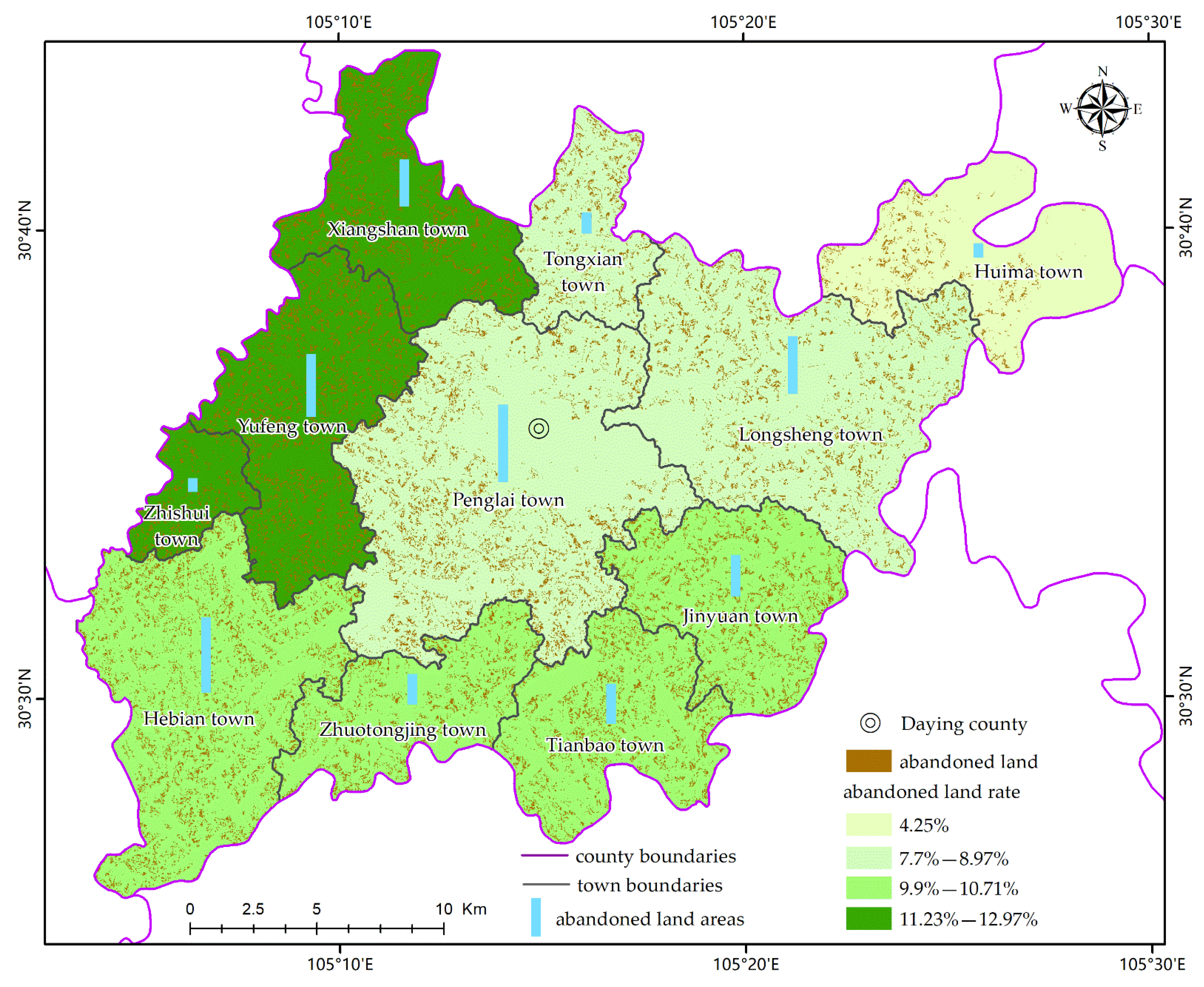
2.1. Study Area
2.2. Data and Preprocessing
2.2.1. Data Source
2.2.2. Data Processing
- (1)
- Projection transformation: MOD09GA and MOD13Q1 images were uniformly transformed into the same projection coordinate system as Sentinel-2 images (WGS 84/ UTM zone 48);
- (2)
- Resample: MOD09GA and MOD13Q1 images in the near-infrared band and red band were resampled to a spatial resolution of 10 m, and the mid-infrared band to 20 m. The method of resample was a bilinear interpolation;
- (3)
- Vector crop: The MOD09GA and MOD13Q1 images were cropped by Sentinel-2, and all images were the same size;
- (4)
- Image registration: The Sentinel-2 image was used as a reference to correct the MOD09GA and MOD13Q1 images;
- (5)
- Band calculation: The ndvi, savi, and ndwi of Sentinel-2 and MOD09GA and MOD13Q1 images were calculated, respectively:
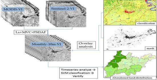
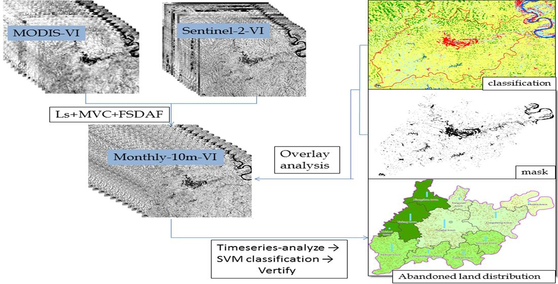
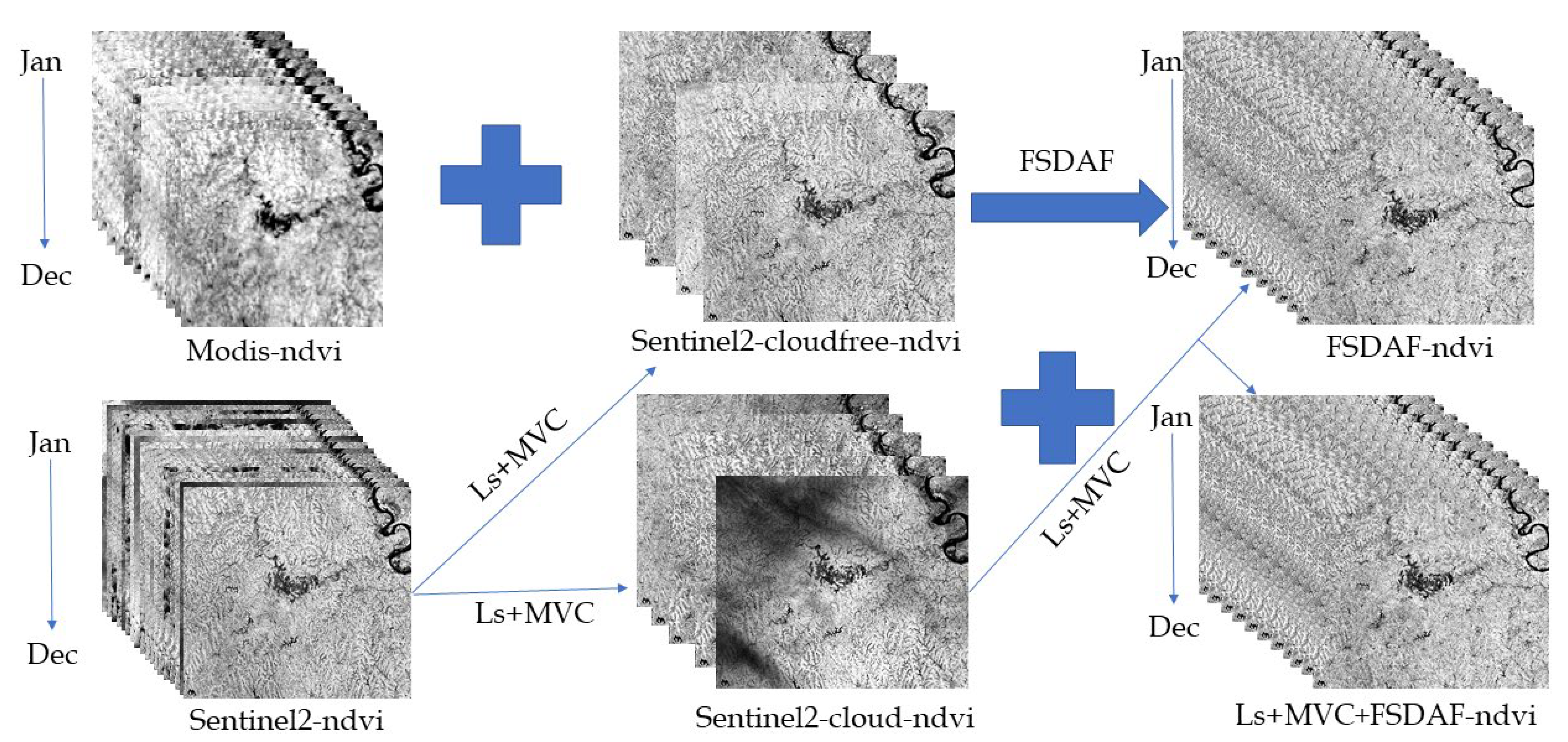
2.3. Data Combining
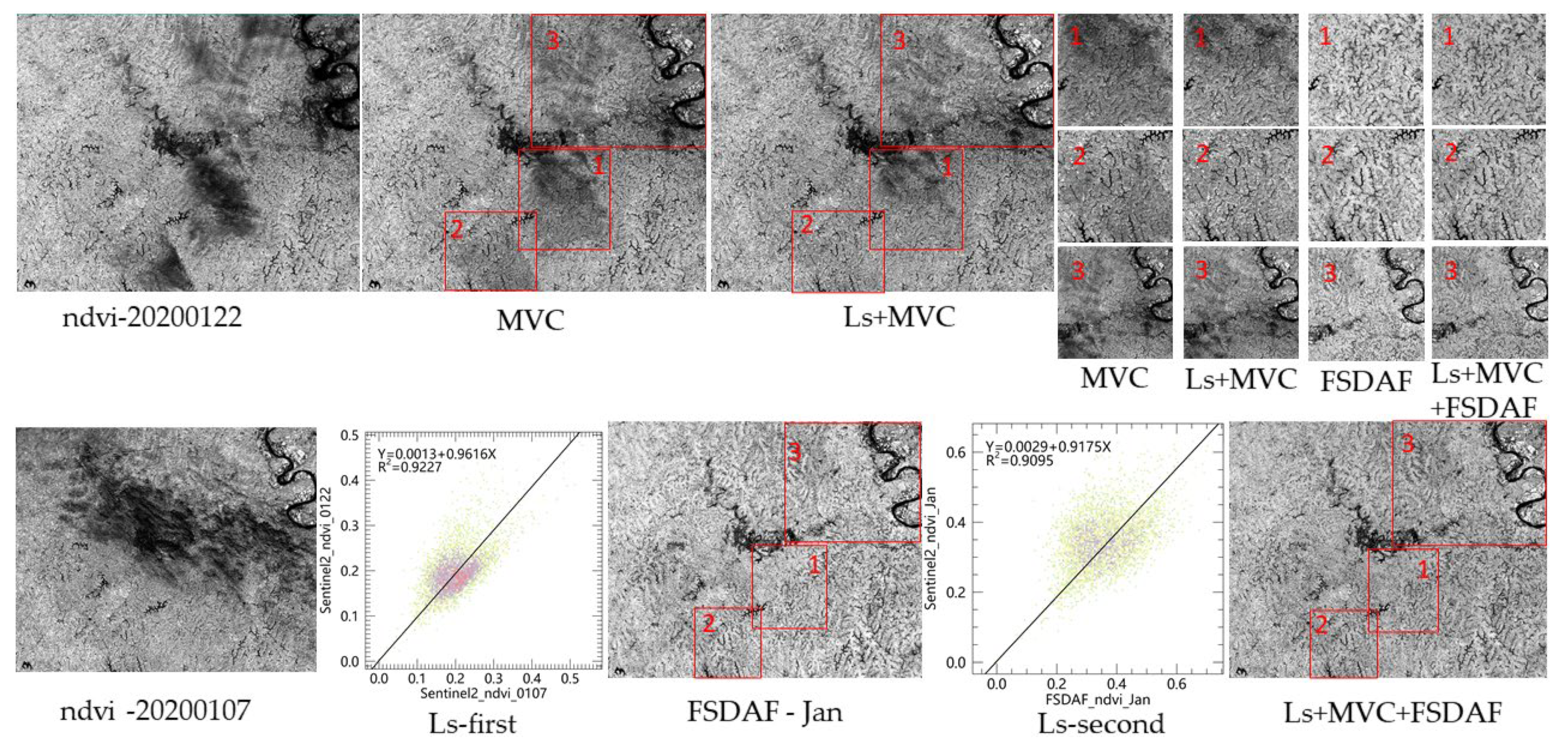
2.3.1. Ls+MVC
2.3.2. FSDAF
2.3.3. Ls+MVC+FSDAF
2.4. SVM Classification
2.5. Accuracy Verification
3. Results
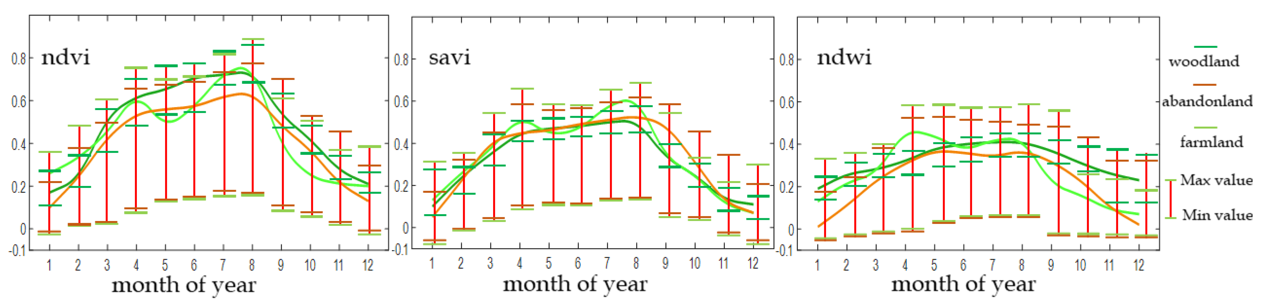
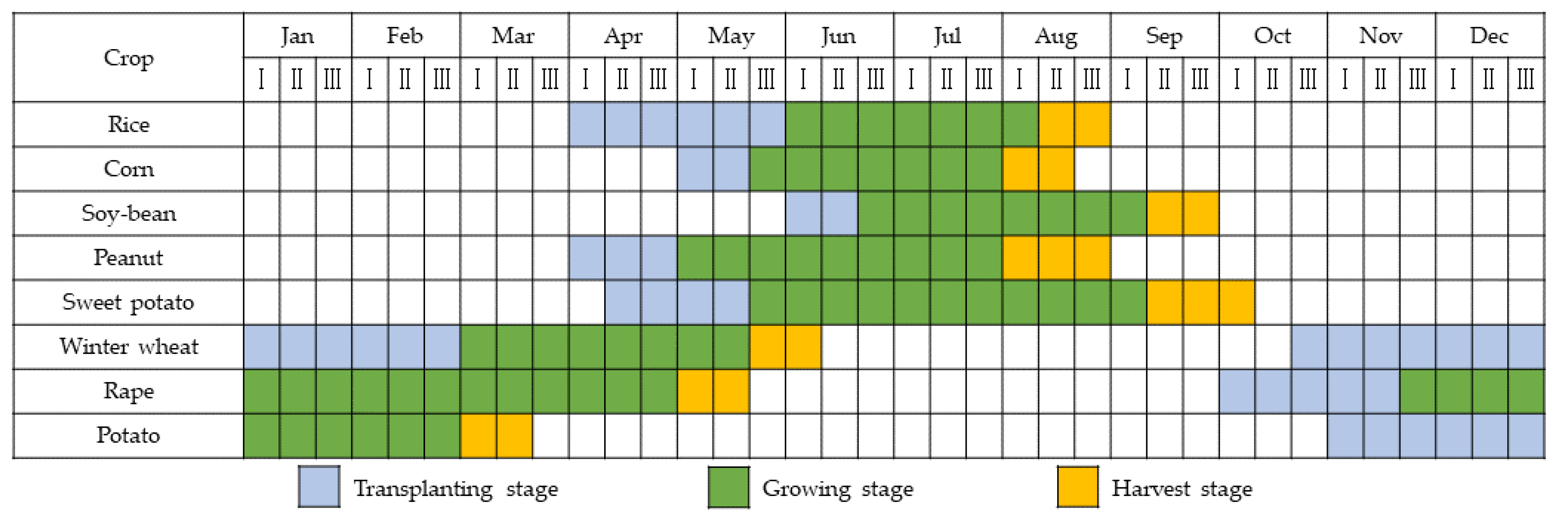
3.1. VIs Time-Series Curve Analysis
3.2. Comparison of Classification Accuracy
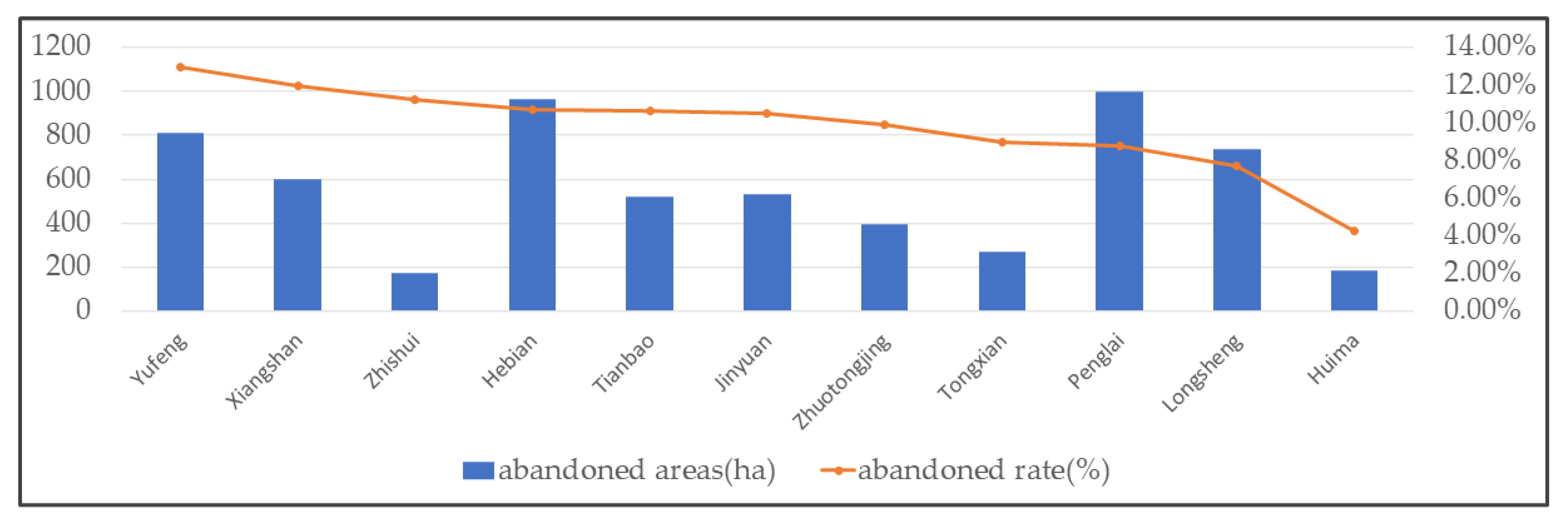
3.3. Abandoned Land Distribution
4. Discussion
4.1. Multi-Source Remote Sensing Image Fusion
4.2. Analysis and Suggestions
4.3. Prospects and Limitations
5. Conclusions
Author Contributions
Funding
Institutional Review Board Statement
Informed Consent Statement
Data Availability Statement
Acknowledgments
Conflicts of Interest
References
- Xu, F.; Ho, H.C.; Chi, G.; Wang, Z. Abandoned rural residential land: Using machine learning techniques to identify rural residential land vulnerable to be abandoned in mountainous areas. Habitat Int. 2019, 84, 43–56. [Google Scholar] [CrossRef]
- Shi, T.; Li, X.; Xin, L.; Xu, X. The spatial distribution of farmland abandonment and its influential factors at the township level: A case study in the mountainous area of China. Land Use Policy 2018, 70, 510–520. [Google Scholar] [CrossRef]
- Xiao, G.; Zhu, X.; Hou, C.; Xia, X. Extraction and analysis of abandoned farmland: A case study of Qingyun and Wudi counties in Shandong Province. J. Geogr. Sci. 2019, 29, 581–597. [Google Scholar] [CrossRef] [Green Version]
- Zhu, X.; Xiao, G.; Zhang, D.; Guo, L. Mapping abandoned farmland in China using time series MODIS NDVI. Sci. Total Environ. 2020, 755 Pt 2, 142651. [Google Scholar]
- Khanal, N.R.; Watanabe, T. Abandonment of agricultural land and its consequences: A case study in the Sikles Area, Gandaki Basin, Nepal Himalaya. Mt. Res. Dev. 2006, 26, 32–40. [Google Scholar] [CrossRef] [Green Version]
- Knoke, T.; Calvas, B.; Moreno, S.O.; Onyekwelu, J.C.; Griess, V.C. Food production and climate protection—What abandoned lands can do to preserve natural forests. Glob. Environ. Chang. 2013, 23, 1064–1072. [Google Scholar] [CrossRef]
- Yoon, H.; Kim, S. Detecting abandoned farmland using harmonic analysis and machine learning. ISPRS J. Photogramm. Remote Sens. 2020, 166, 201–212. [Google Scholar] [CrossRef]
- Feng, G.; Masek, J.; Schwaller, M.; Hall, F. On the blending of the Landsat and MODIS surface reflectance: Predicting daily Landsat surface reflectance. IEEE Trans. Geosci. Remote Sens. 2006, 44, 2207–2218. [Google Scholar] [CrossRef]
- Houborg, R.; McCabe, M.F.; Gao, F. A spatio-temporal enhancement method for medium resolution LAI (STEM-LAI). Int. J. Appl. Earth Obs. Geoinf. 2016, 47, 15–29. [Google Scholar] [CrossRef] [Green Version]
- Mizuochi, H.; Hiyama, T.; Ohta, T.; Fujioka, Y.; Kambatuku, J.R.; Iijima, M.; Nasahara, K.N. Development and evaluation of a lookup-table-based approach to data fusion for seasonal wetlands monitoring: An integrated use of AMSR series, MODIS, and Landsat. Remote Sens. Environ. 2017, 199, 370–388. [Google Scholar] [CrossRef]
- Tian, F.; Wang, Y.; Fensholt, R.; Wang, K.; Zhang, L.; Huang, Y. Mapping and Evaluation of NDVI Trends from Synthetic Time Series Obtained by Blending Landsat and MODIS Data around a Coalfield on the Loess Plateau. Remote Sens. 2013, 5, 4255–4279. [Google Scholar] [CrossRef] [Green Version]
- Zhang, F.; Zhu, X.; Liu, D. Blending MODIS and Landsat images for urban flood mapping. Int. J. Remote Sens. 2014, 35, 3237–3253. [Google Scholar] [CrossRef]
- Zurita-Milla, R.; Clevers, J.; Schaepman, M.E. Unmixing-Based Landsat TM and MERIS FR Data Fusion. IEEE Geosci. Remote Sens. Lett. 2008, 5, 453–457. [Google Scholar] [CrossRef] [Green Version]
- Roy, D.P.; Ju, J.; Lewis, P.; Schaaf, C.; Gao, F.; Hansen, M.; Lindquist, E. Multi-temporal MODIS–Landsat data fusion for relative radiometric normalization, gap filling, and prediction of Landsat data. Remote Sens. Environ. 2008, 112, 3112–3130. [Google Scholar] [CrossRef]
- Hilker, T.; Wulder, M.A.; Coops, N.C.; Linke, J.; McDermid, G.; Masek, J.G.; Gao, F.; White, J.C. A new data fusion model for high spatial- and temporal-resolution mapping of forest disturbance based on Landsat and MODIS. Remote Sens. Environ. 2009, 113, 1613–1627. [Google Scholar] [CrossRef]
- Zhu, X.; Chen, J.; Gao, F.; Chen, X.; Masek, J.G. An enhanced spatial and temporal adaptive reflectance fusion model for complex heterogeneous regions. Remote Sens. Environ. 2010, 114, 2610–2623. [Google Scholar] [CrossRef]
- Song, H.; Huang, B. Spatiotemporal Satellite Image Fusion Through One-Pair Image Learning. IEEE Trans. Geosience Remote Sens. 2013, 51, 1883–1896. [Google Scholar] [CrossRef]
- Gao, F.; Hilker, T.; Zhu, X.; Anderson, M.; Masek, J.; Wang, P.; Yang, Y. Fusing Landsat and MODIS Data for Vegetation Monitoring. IEEE Geosci. Remote Sens. Mag. 2015, 3, 47–60. [Google Scholar] [CrossRef]
- Rao, Y.; Zhu, X.; Chen, J.; Wang, J. An Improved Method for Producing High Spatial-Resolution NDVI Time Series Datasets with Multi-Temporal MODIS NDVI Data and Landsat TM/ETM+ Images. Remote Sens. 2015, 7, 7865–7891. [Google Scholar] [CrossRef] [Green Version]
- Zhu, X.; Helmer, E.H.; Gao, F.; Liu, D.; Chen, J.; Lefsky, M.A. A flexible spatiotemporal method for fusing satellite images with different resolutions. Remote Sens. Environ. 2016, 172, 165–177. [Google Scholar] [CrossRef]
- Zhu, X.; Cai, F.; Tian, J.; Williams, T.K.-A. Spatiotemporal Fusion of Multisource Remote Sensing Data: Literature Survey, Taxonomy, Principles, Applications, and Future Directions. Remote Sens. 2018, 10, 527. [Google Scholar] [CrossRef] [Green Version]
- Liu, M.; Ke, Y.; Yin, Q.; Chen, X.; Im, J. Comparison of Five Spatio-Temporal Satellite Image Fusion Models over Landscapes with Various Spatial Heterogeneity and Temporal Variation. Remote Sens. 2019, 11, 2612. [Google Scholar] [CrossRef] [Green Version]
- Zhou, J.; Chen, J.; Chen, X.; Zhu, X.; Qiu, Y.; Song, H.; Rao, Y.; Zhang, C.; Cao, X.; Cui, X. Sensitivity of six typical spatiotemporal fusion methods to different influential factors: A comparative study for a normalized difference vegetation index time series reconstruction. Remote Sens. Environ. 2021, 252, 112130. [Google Scholar] [CrossRef]
- Liu, M.; Yang, W.; Zhu, X.; Chen, J.; Chen, X.; Yang, L.; Helmer, E.H. An Improved Flexible Spatiotemporal DAta Fusion (IFSDAF) method for producing high spatiotemporal resolution normalized difference vegetation index time series. Remote Sens. Environ. 2019, 227, 74–89. [Google Scholar] [CrossRef]
- Chen, X.; Liu, M.; Zhu, X.; Chen, J.; Zhong, Y.; Cao, X. "Blend-then-Index" or "Index-then-Blend": A theoretical analysis for Generating High-resolution NDVI Time Series by STARFM. Photogramm. Eng. Remote Sens. 2018, 84, 65–73. [Google Scholar] [CrossRef]
- Zhang, X.; Liu, L.; Chen, X.; Gao, Y.; Xie, S.; Mi, J. GLC_FCS30: Global land-cover product with fine classification system at 30 m using time-series Landsat imagery. Earth Syst. Sci. Data 2021, 13, 2753–2776. [Google Scholar] [CrossRef]
- Zhang, X.; Liu, L.; Wu, C.; Chen, X.; Gao, Y.; Xie, S.; Zhang, B. Development of a global 30 m impervious surface map using multisource and multitemporal remote sensing datasets with the Google Earth Engine platform. Earth Syst. Sci. Data 2020, 12, 1625–1648. [Google Scholar] [CrossRef]
- Zhang, X.; Liu, L.; Chen, X.; Xie, S.; Gao, Y. Fine Land-Cover Mapping in China Using Landsat Datacube and an Operational SPECLib-Based Approach. Remote Sens. 2019, 11, 1056. [Google Scholar] [CrossRef] [Green Version]
- Xie, S.; Liu, L.; Zhang, X.; Yang, J.; Gao, Y. Automatic land-cover mapping using Landsat time-series data based on Google Earth Engine. 2019, 11, 3023. Remote Sens. 2019, 11, 3023. [Google Scholar] [CrossRef] [Green Version]
- Gao, Y.; Liu, L.; Zhang, X.; Chen, X.; Xie, S. Consistency analysis and accuracy assessment of three global 30-m Land-Cover products over the European Union using the LUCAS Dataset. Remote Sens. 2020, 12, 3479. [Google Scholar] [CrossRef]
- Löw, F.; Prishchepov, A.V.; Waldner, F.; Dubovyk, O.; Akramkhanov, A.; Biradar, C.; Lamers, J.P. Mapping cropland abandonment in the Aral Sea Basin with MODIS time series. Remote Sens. 2018, 10, 159. [Google Scholar] [CrossRef] [Green Version]
- Lesiv, M.; Schepaschenko, D.; Moltchanova, E.; Bun, R.; Dürauer, M.; Prishchepov, A.V.; Schierhorn, F.; Estel, S.; Kuemmerle, T.; Alcántara, C. Spatial distribution of arable and abandoned land across former Soviet Union countries. Sci. Data 2018, 5, 180056. [Google Scholar] [CrossRef]
- Tong, X.; Brandt, M.; Hiernaux, P.; Herrmann, S.M.; Tian, F.; Prishchepov, A.V.; Fensholt, R. Revisiting the coupling between NDVI trends and cropland changes in the Sahel drylands: A case study in western Niger. Remote Sens. Environ. 2017, 191, 286–296. [Google Scholar] [CrossRef] [Green Version]
- Estel, S.; Kuemmerle, T.; Levers, C.; Baumann, M.; Hostert, P. Mapping cropland-use intensity across Europe using MODIS NDVI time series. Environ. Res. Lett. 2016, 11, 024015. [Google Scholar] [CrossRef] [Green Version]
- Estel, S.; Kuemmerle, T.; Alcántara, C.; Levers, C.; Prishchepov, A.; Hostert, P. Mapping farmland abandonment and recultivation across Europe using MODIS NDVI time series. Remote Sens. Environ. 2015, 163, 312–325. [Google Scholar] [CrossRef]
- Alcantara, C.; Kuemmerle, T.; Baumann, M.; Bragina, E.V.; Griffiths, P.; Hostert, P.; Knorn, J.; Müller, D.; Prishchepov, A.V.; Schierhorn, F.; et al. Mapping the extent of abandoned farmland in Central and Eastern Europe using MODIS time series satellite data. Environ. Res. Lett. 2013, 8, 035035. [Google Scholar] [CrossRef]
- Alcantara, C.; Kuemmerle, T.; Prishchepov, A.V.; Radeloff, V.C. Mapping abandoned agriculture with multi-temporal MODIS satellite data. Remote Sens. Environ. 2012, 124, 334–347. [Google Scholar] [CrossRef]
- Schweers, W.; Bai, Z.; Campbell, E.; Hennenberg, K.; Fritsche, U.; Mang, H.P.; Lucas, M.; Li, Z.; Scanlon, A.; Chen, H. Identification of potential areas for biomass production in China: Discussion of a recent approach and future challenges. Biomass Bioenergy 2011, 35, 2268–2279. [Google Scholar] [CrossRef]
- Yin, H.; Prishchepov, A.V.; Kuemmerle, T.; Bleyhl, B.; Buchner, J.; Radeloff, V.C. Mapping agricultural land abandonment from spatial and temporal segmentation of Landsat time series. Remote Sens. Environ. 2018, 210, 12–24. [Google Scholar] [CrossRef]
- Yusoff, N.M.; Muharam, F.M.; Khairunniza-Bejo, S. Towards the use of remote-sensing data for monitoring of abandoned oil palm lands in Malaysia: A semi-automatic approach. Int. J. Remote Sens. 2017, 38, 432–449. [Google Scholar] [CrossRef]
- Cvitanović, M.; Lučev, I.; Fürst-Bjeliš, B.; Borčić, S.L.; Horvat, S.; Valozic, L. Analyzing post-socialist grassland conversion in a traditional agricultural landscape–Case study Croatia. J. Rural. Stud. 2017, 51, 53–63. [Google Scholar] [CrossRef] [Green Version]
- Löw, F.; Fliemann, E.; Abdullaev, I.; Conrad, C.; Lamers, J.P.A. Mapping abandoned agricultural land in Kyzyl-Orda, Kazakhstan using satellite remote sensing. Appl. Geogr. 2015, 62, 377–390. [Google Scholar] [CrossRef]
- Goodin, D.G.; Anibas, K.L.; Bezymennyi, M. Mapping land cover and land use from object-based classification: An example from a complex agricultural landscape. Int. J. Remote Sens. 2015, 36, 4702–4723. [Google Scholar] [CrossRef]
- Kanianska, R.; Kizeková, M.; Novácek, J.; Zeman, M. Land-use and land-cover changes in rural areas during different political systems: A case study of Slovakia from 1782 to 2006. Land Use Policy 2014, 36, 554–566. [Google Scholar] [CrossRef]
- Prishchepov, A.; Müller, D.; Dubinin, M.; Baumann, M.; Radeloff, V.C. Determinants of agricultural land abandonment in post-Soviet European Russia. Land Use Policy 2013, 30, 873–884. [Google Scholar] [CrossRef] [Green Version]
- Müller, D.; Leito, P.J.; Sikor, T. Comparing the determinants of cropland abandonment in Albania and Romania using boosted regression trees. Agric. Syst. 2013, 117, 66–77. [Google Scholar] [CrossRef]
- Prishchepov, A.V.; Radeloff, V.C.; Dubinin, M.; Alcantara, C. The effect of Landsat ETM/ETM + image acquisition dates on the detection of agricultural land abandonment in Eastern Europe. Remote Sens. Environ. 2012, 126, 195–209. [Google Scholar] [CrossRef]
- Prishchepov, A.V.; Radeloff, V.C.; Baumann, M.; Kuemmerle, T.; Müller, D. Effects of institutional changes on land use: Agricultural land abandonment during the transition from state-command to market-driven economies in post-Soviet Eastern Europe. Environ. Res. Lett. 2012, 7, 024021. [Google Scholar] [CrossRef]
- Kuemmerle, T.; Olofsson, P.; Chaskovskyy, O.; Baumann, M.; Ostapowicz, K.; Woodcock, C.E.; Houghton, R.A.; Hostert, P.; Keeton, W.S.; Radeloff, V.C. Post-Soviet farmland abandonment, forest recovery, and carbon sequestration in western Ukraine. Glob. Chang. Biol. 2011, 17, 1335–1349. [Google Scholar] [CrossRef]
- Kuemmerle, T.; Müller, D.; Griffiths, P.; Rusu, M. Land use change in Southern Romania after the collapse of socialism. Reg. Environ. Chang. 2009, 9, 1–12. [Google Scholar] [CrossRef]
- Kuemmerle, T.; Hostert, P.; Radeloff, V.C.; Linden, S.; Perzanowski, K.; Kruhlov, I. Cross-border Comparison of Post-socialist Farmland Abandonment in the Carpathians. Ecosystems 2008, 11, 614–628. [Google Scholar] [CrossRef]
- Witmer, F.D.W. Detecting war-induced abandoned agricultural land in northeast Bosnia using multispectral, multitemporal Landsat TM imagery. Int. J. Remote Sens. 2008, 29, 3805–3831. [Google Scholar] [CrossRef]
- Müller, D.; Sikor, T. Effects of postsocialist reforms on land cover and land use in South-Eastern Albania. Appl. Geogr. 2006, 26, 175–191. [Google Scholar] [CrossRef]
- Peterson, U.; Aunap, R. Changes in agricultural land use in Estonia in the 1990s detected with multitemporal Landsat MSS imagery. Landsc. Urban Plan. 1998, 41, 193–201. [Google Scholar] [CrossRef]
- Milenov, P.; Vassilev, V.; Vassileva, A.; Radkov, R.; Samoungi, V.; Dimitrov, Z.; Vichev, N. Monitoring of the risk of farmland abandonment as an efficient tool to assess the environmental and socio-economic impact of the Common Agriculture Policy. Int. J. Appl. Earth Obs. Geoinf. 2014, 32, 218–227. [Google Scholar] [CrossRef]
- Wang, S.; Li, W.; Zhou, Y.; Wang, F.; Xu, Q. Object-oriented Classification Technique for Extracting Abandoned Farmlands by Using Remote Sensing Images. Int. Conf. Multimed. Technol. 2013, 1497–2504. [Google Scholar]
- Günthert, S.; Siegmund, A.; Thunig, H.; Michel, U. Object-based detection of LUCC with special regard to agricultural abandonment on Tenerife (Canary Islands). Earth Resour. Environ. Remote Sens. /GIS Appl. 2011, 13, 33. [Google Scholar]
- Scihub.Copernicus. 2021. Available online: https://scihub.copernicus.eu/dhus/#/home (accessed on 7 May 2021).
- Earthexplorer.USGS. 2021. Available online: http://earthexplorer.usgs.gov (accessed on 3 May 2021).
- The Earth Science Big Data Science Engineering Data Sharing Service System. 2021. Available online: http://data.casearth.cn/sdo/detail/5fbc7904819aec1ea2dd7061 (accessed on 21 May 2021).
- Openstreetmap. 2021. Available online: https://download.geofabrik.de/asia.html (accessed on 24 May 2021).
- Hao, P.; Zhan, Y.; Wang, L.; Niu, Z.; Shakir, M. Feature Selection of Time Series MODIS Data for Early Crop Classification Using Random Forest: A Case Study in Kansas, USA. Remote Sens. 2015, 7, 5347–5369. [Google Scholar] [CrossRef] [Green Version]
- Holben, B.N. Characteristics of maximum-value composite images from temporal AVHRR data. Int. J. Remote Sens. 1986, 7, 1417–1434. [Google Scholar] [CrossRef]
- Huete, A.; Didan, K.; Miura, T.; Rodriguez, E.P.; Gao, X.; Ferreira, L.G. Overview of the radiometric and biophysical performance of the MODIS vegetation indices. Remote Sens. Environ. 2002, 83, 195–213. [Google Scholar] [CrossRef]
- Roy, D.P.; Ju, J.; Kline, K.; Scaramuzza, P.L.; Kovalskyy, V.; Hansen, M.; Loveland, T.R.; Vermote, E.; Zhang, C. Web-enabled Landsat Data (WELD): Landsat ETM+ composited mosaics of the conterminous United States. Remote Sens. Environ. 2010, 114, 35–49. [Google Scholar] [CrossRef]
- Tai, S.C.; Chen, P.Y.; Chao, C.Y. Missing pixels restoration for remote sensing images using adaptive search window and linear regression. J. Electron. Imaging 2016, 25, 043017. [Google Scholar] [CrossRef]
- Xie, D.; Gao, F.; Sun, L.; Anderson, M. Improving Spatial-Temporal Data Fusion by Choosing Optimal Input Image Pairs. Remote Sens. 2018, 10, 1142. [Google Scholar] [CrossRef] [Green Version]
- Jiang, J.; Zhang, Q.; Yao, X.; Tian, Y.; Zhu, Y.; Cao, W.; Cheng, T. HISTIF: A New Spatiotemporal Image Fusion Method for High-Resolution Monitoring of Crops at the Subfield Level. IEEE J. Sel. Top. Appl. Earth Obs. Remote Sens. 2020, 13, 4607–4626. [Google Scholar] [CrossRef]
- Gao, H.; Zhu, X.; Guan, Q.; Yang, X.; Peng, X. cuFSDAF: An Enhanced Flexible Spatiotemporal Data Fusion Algorithm Parallelized Using Graphics Processing Units. IEEE Trans. Geosci. Remote Sens. 2021, 99, 1–16. [Google Scholar]
- Gorelick, N.; Hancher, M.; Dixon, M.; Ilyushchenko, S.; Thau, D.; Moore, R. Google Earth Engine: Planetary-scale geospatial analysis for everyone. Remote Sens. Environ. 2017, 202, 18–27. [Google Scholar] [CrossRef]
- Pan, L.; Xia, H.; Yang, J.; Niu, W.; Wang, R.; Song, H.; Guo, Y.; Qin, Y. Mapping cropping intensity in Huaihe basin using phenology algorithm, all Sentinel-2 and Landsat images in Google Earth Engine. Int. J. Appl. Earth Obs. Geoinf. 2021, 102, 102376. [Google Scholar] [CrossRef]
- Pan, L.; Xia, H.; Zhao, X.; Guo, Y.; Qin, Y. Mapping Winter Crops Using a Phenology Algorithm, Time-Series Sentinel-2 and Landsat-7/8 Images, and Google Earth Engine. Remote Sens. 2021, 13, 2510. [Google Scholar] [CrossRef]


| Used Remote Sensing Data | Number of Studies | Study IDs |
|---|---|---|
| MODIS | 9 | [4,31,32,33,34,35,36,37,38] |
| Landsat | 17 | [3,39,40,41,42,43,44,45,46,47,48,49,50,51,52,53,54] |
| Sentinel-2 | 1 | [7] |
| SPOT | 2 | [55,56] |
| RapidEye | 1 | [57] |
| Remote Sensing Type | Band Number | Band Range (nm) | Spatio-temporal Resolution (d/m) |
|---|---|---|---|
| Sentinel-2 | Band 4—Red | 650–680 | 5/10 |
| Band 8—NIR | 785–900 | 5/10 | |
| Band 12—SWIR | 2100–2280 | 5/20 | |
| MOD09GA | Band 1—Red | 620–670 | 1/250 |
| Band 2—NIR | 841–876 | 1/250 | |
| Band 7—SWIR | 2105–2155 | 1/500 | |
| MOD13Q1 | ndvi | - | 16/250 |
| Band 1—Red | 620–670 | 16/250 | |
| Band 2—NIR | 841–876 | 16/250 | |
| Band 7—SWIR | 2105–2155 | 16/500 |
| Remote Sensing Image Data Source | Overall Accuracy | User Accuracy | Product Accuracy | Kappa Coefficient |
|---|---|---|---|---|
| Sentinel-2 (August, November) | 64.5% | 54.5% | 57.6% | 0.58 |
| Ls+MVC (March, June, August, November) | 77.3% | 72.7% | 81.4% | 0.73 |
| Ls+MVC+FSDAF (January to December) | 88.1% | 94.1% | 86.5% | 0.87 |
| Fusion Method | Basic Image | S20201112 Cloud Content | R2 | RMSE |
|---|---|---|---|---|
| MVC | S20201107 S20201112 | 20% | 0.9155 | 0.0321 |
| 40% | 0.9044 | 0.0326 | ||
| 60% | 0.8988 | 0.0328 | ||
| 80% | 0.8939 | 0.0331 | ||
| Ls+MVC | S20201112 S20201107 | 20% | 0.9311 | 0.0192 |
| 40% | 0.9122 | 0.0214 | ||
| 60% | 0.9020 | 0.0227 | ||
| 80% | 0.8947 | 0.0236 | ||
| FSDAF | M20201112 S20201107 S20201112 | 20% | 0.8766 | 0.0274 |
| 40% | ||||
| 60% |
Publisher’s Note: MDPI stays neutral with regard to jurisdictional claims in published maps and institutional affiliations. |
© 2021 by the authors. Licensee MDPI, Basel, Switzerland. This article is an open access article distributed under the terms and conditions of the Creative Commons Attribution (CC BY) license (https://creativecommons.org/licenses/by/4.0/).
Share and Cite
He, S.; Shao, H.; Xian, W.; Zhang, S.; Zhong, J.; Qi, J. Extraction of Abandoned Land in Hilly Areas Based on the Spatio-Temporal Fusion of Multi-Source Remote Sensing Images. Remote Sens. 2021, 13, 3956. https://doi.org/10.3390/rs13193956
He S, Shao H, Xian W, Zhang S, Zhong J, Qi J. Extraction of Abandoned Land in Hilly Areas Based on the Spatio-Temporal Fusion of Multi-Source Remote Sensing Images. Remote Sensing. 2021; 13(19):3956. https://doi.org/10.3390/rs13193956
Chicago/Turabian StyleHe, Shan, Huaiyong Shao, Wei Xian, Shuhui Zhang, Jialong Zhong, and Jiaguo Qi. 2021. "Extraction of Abandoned Land in Hilly Areas Based on the Spatio-Temporal Fusion of Multi-Source Remote Sensing Images" Remote Sensing 13, no. 19: 3956. https://doi.org/10.3390/rs13193956
APA StyleHe, S., Shao, H., Xian, W., Zhang, S., Zhong, J., & Qi, J. (2021). Extraction of Abandoned Land in Hilly Areas Based on the Spatio-Temporal Fusion of Multi-Source Remote Sensing Images. Remote Sensing, 13(19), 3956. https://doi.org/10.3390/rs13193956