Author Contributions
Conceptualization M.D., K.V., I.S.; Data annotation O.W, F.H.; Model development M.D.; Software I.S., H.T., A.K., M.V., T.T.; Writing—original draft M.D.; Writing—review and editing I.S., O.W., A.O., M.J., E.G.C., N.L., T.T.; Project administration M.D., K.V., M.J., V.B., Supervision—V.B., N.L., E.G.C., Resources—T.T., E.G.C. All authors have read and agreed to the published version of the manuscript.
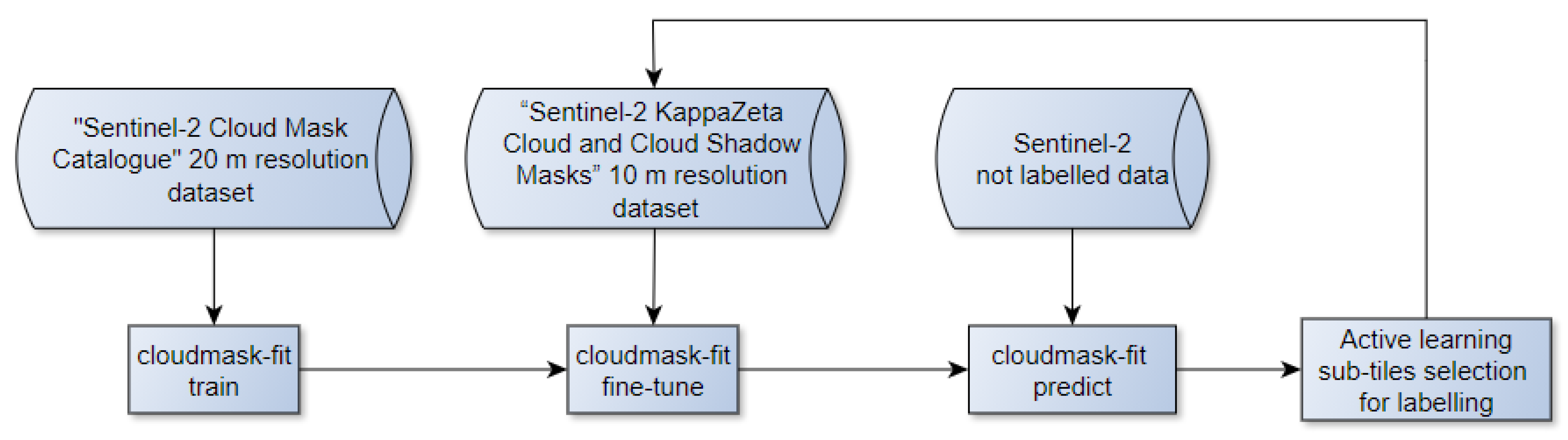
Figure 1.
General pipeline of the KappaMask model development.
Figure 1.
General pipeline of the KappaMask model development.
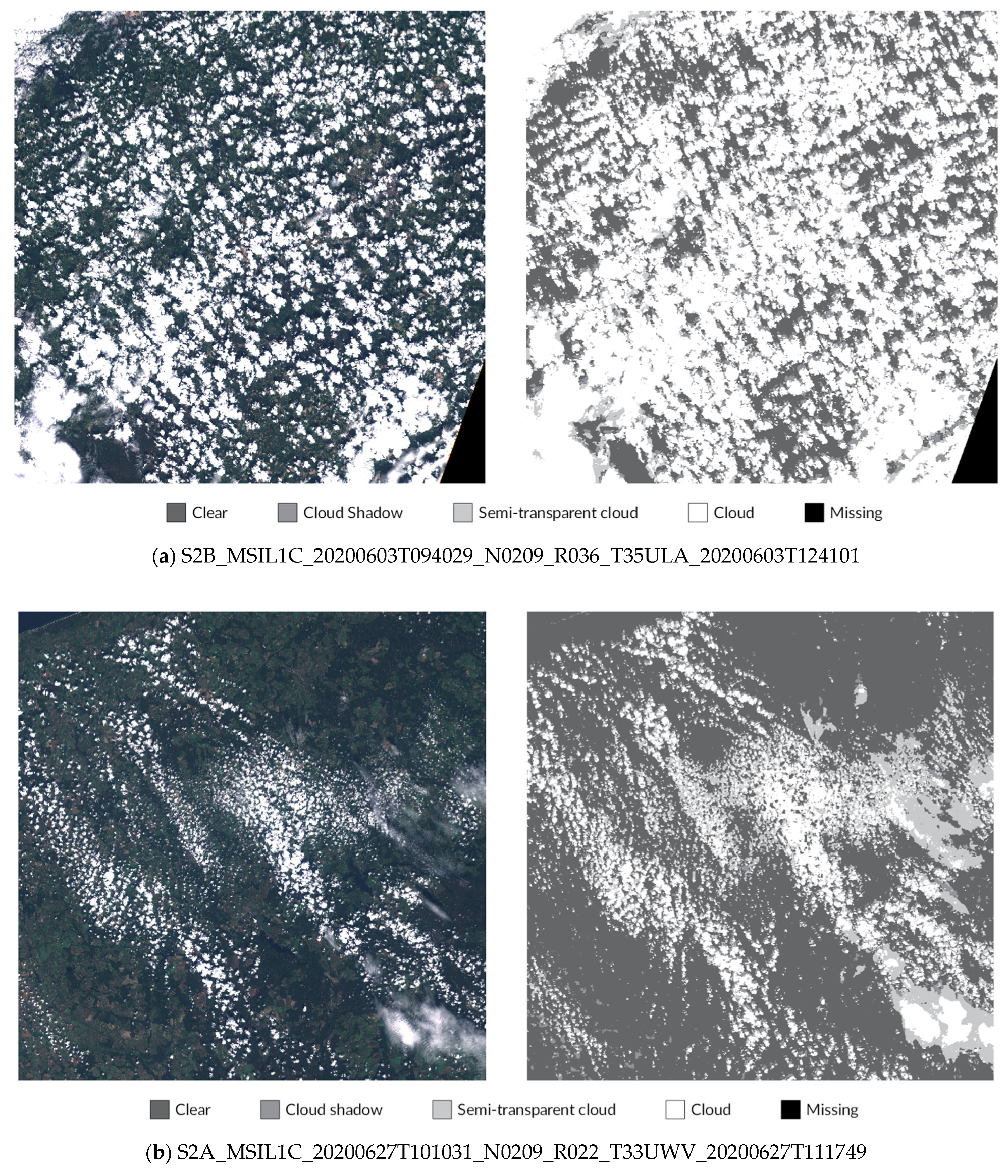
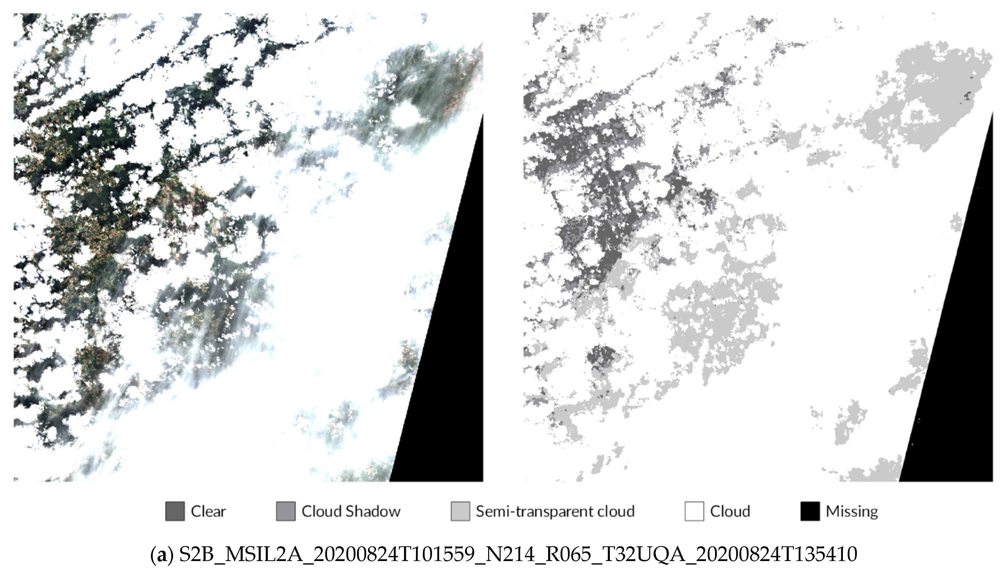
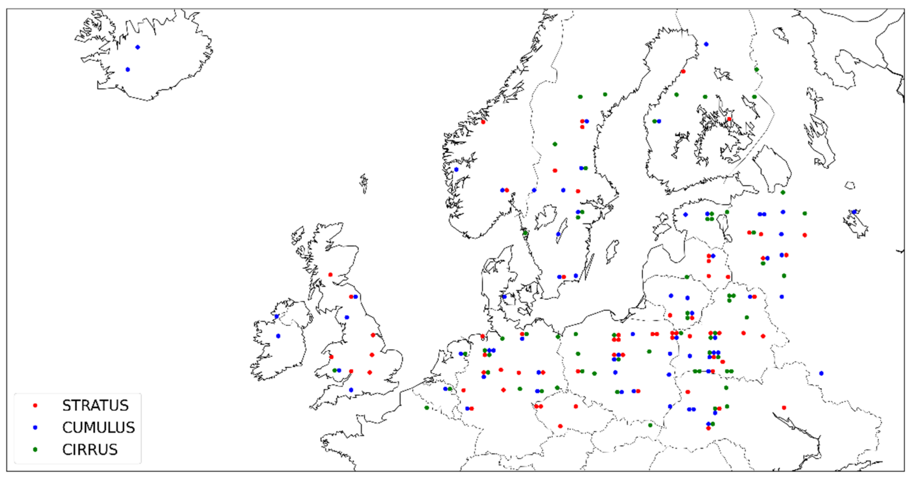
Figure 2.
Sentinel-2 tiles used for labelling. Images with cumulus clouds are indicated as blue dots, images with stratus clouds are marked as red and images with cirrus clouds are marked as green. Each dot corresponds to one Sentinel-2 100 × 100 km data product. If the dots are exactly next to each other, it means the corresponding Sentinel-2 products are from the same location.
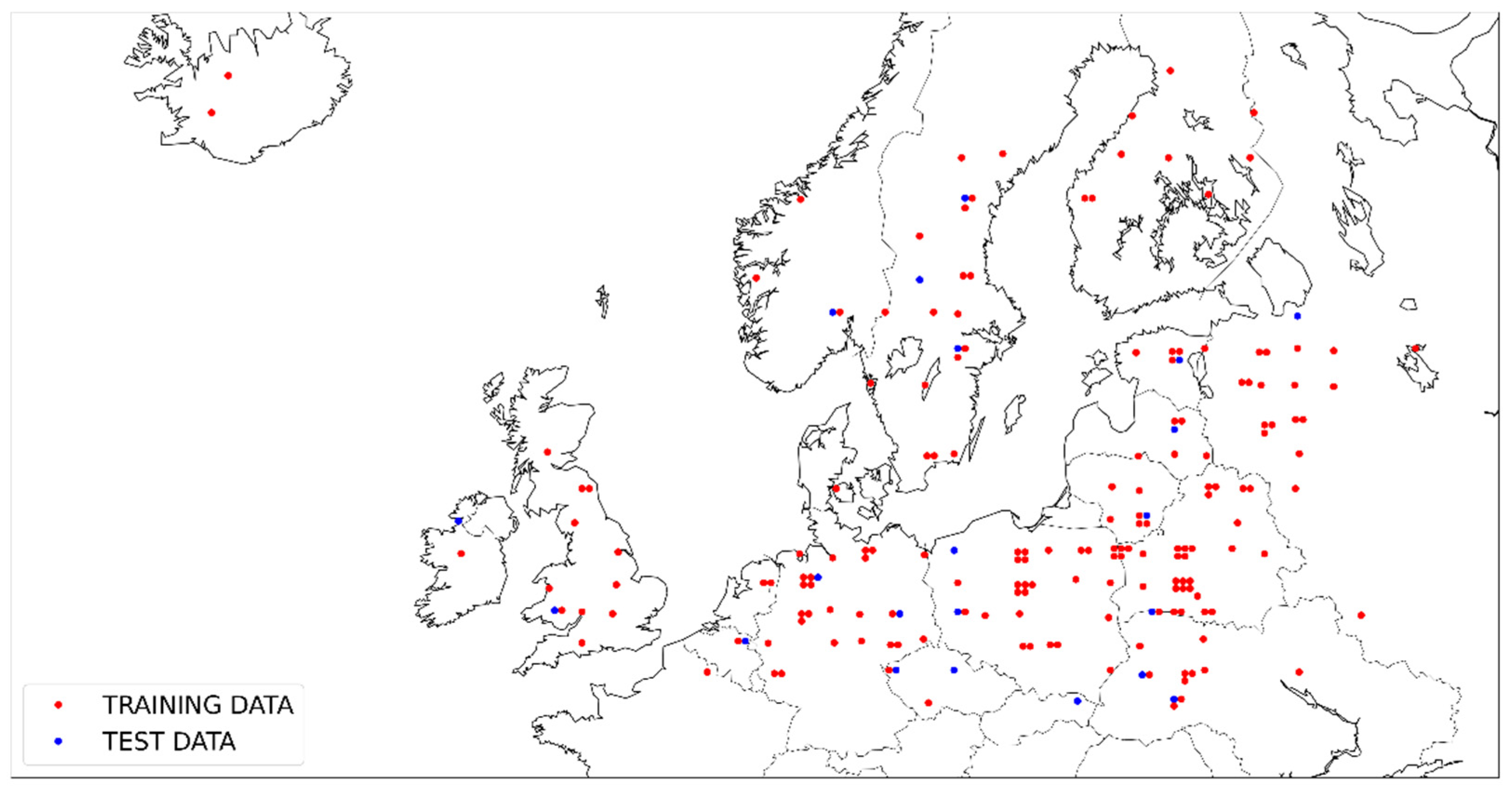
Figure 3.
Distribution of the training and test data. Red dots indicate Sentinel-2 images reserved for training and validation dataset, and blue dots indicate images used for the test dataset only. If the dots are exactly next to each other, it means the corresponding Sentinel-2 products are from the same location.
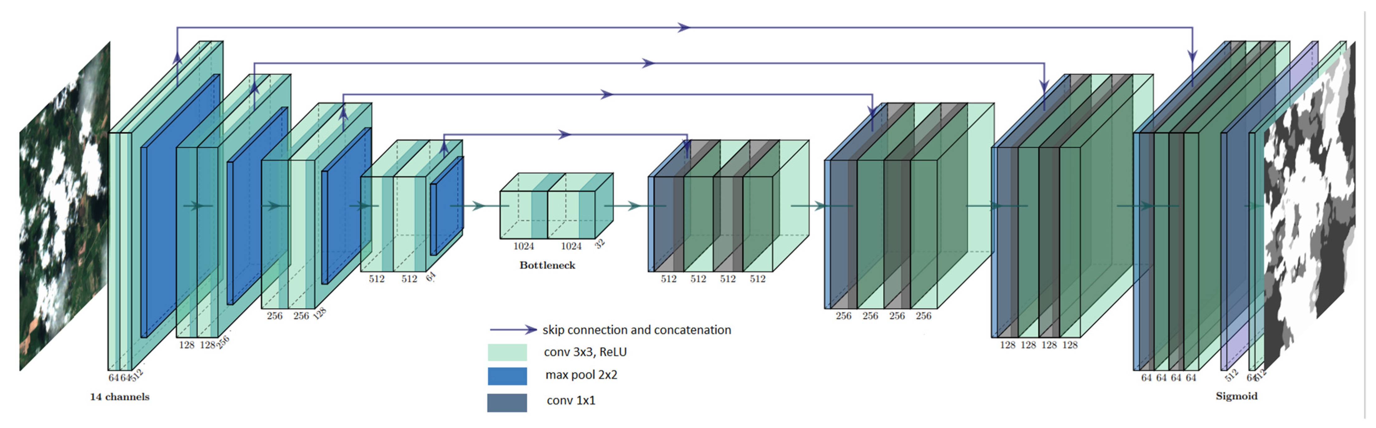
Figure 4.
U-Net model architecture used for training.
Figure 4.
U-Net model architecture used for training.
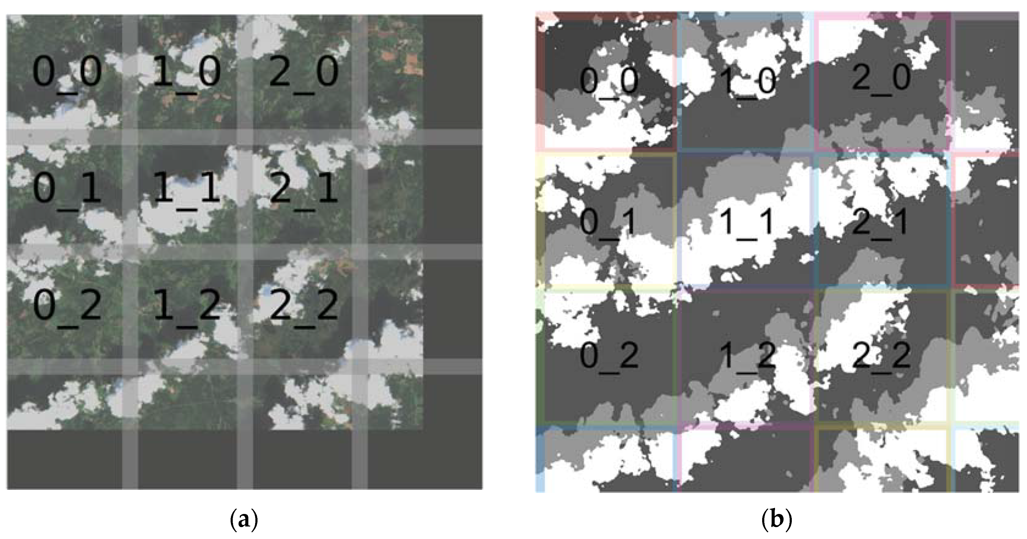
Figure 5.
Illustrative images of how full Sentinel-2 image is cropped for prediction and how classification map is rebuilt into the full image with 32 pixels overlap. (a) Cropping original Sentinel-2 image for inference. (b) Prediction output mask combined into the final image.
Figure 5.
Illustrative images of how full Sentinel-2 image is cropped for prediction and how classification map is rebuilt into the full image with 32 pixels overlap. (a) Cropping original Sentinel-2 image for inference. (b) Prediction output mask combined into the final image.
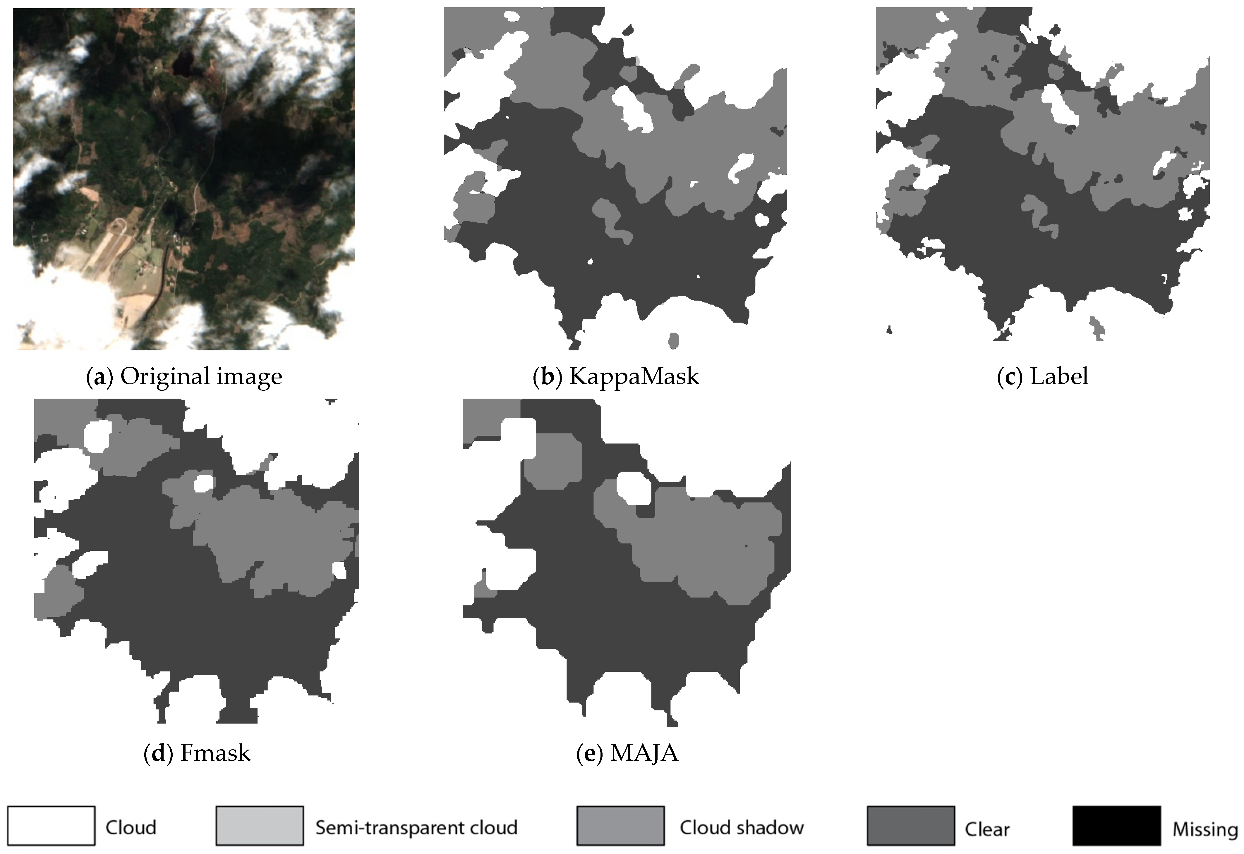
Figure 6.
Comparison of L2A prediction output for a 512 × 512 pixels sub-tile in the test dataset. (a) Original Sentinel-2 L2A True-Color Image; (b) KappaMask classification map; (c) Segmentation mask prepared by a human labeller; (d) Fmask classification map; (e) MAJA classification map.
Figure 6.
Comparison of L2A prediction output for a 512 × 512 pixels sub-tile in the test dataset. (a) Original Sentinel-2 L2A True-Color Image; (b) KappaMask classification map; (c) Segmentation mask prepared by a human labeller; (d) Fmask classification map; (e) MAJA classification map.
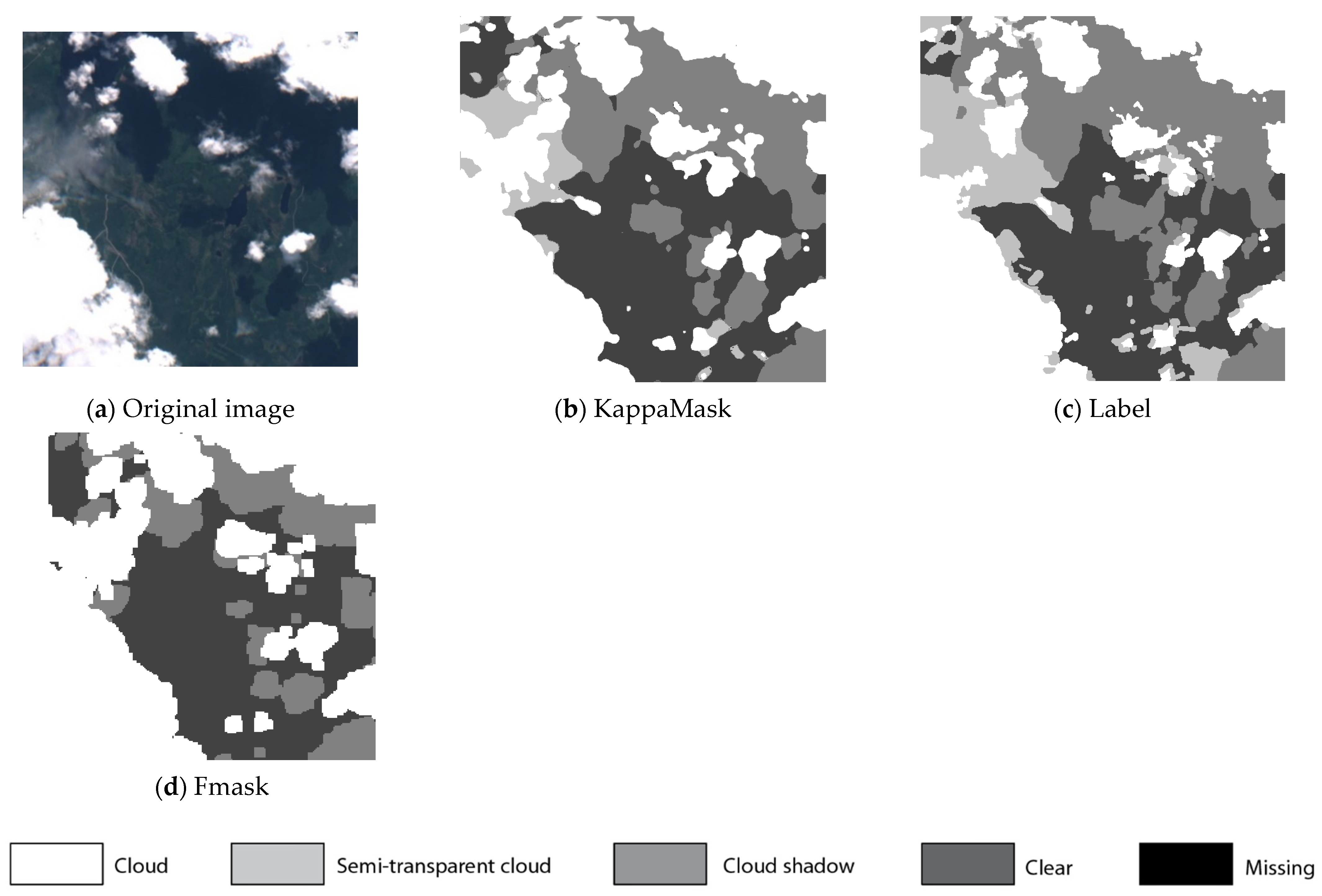
Figure 7.
Comparison of L1C prediction output for a 512 × 512 pixels sub-tile in the test dataset. (a) Original Sentinel-2 L1C True-Colour Image; (b) KappaMask classification map; (c) Segmentation mask prepared by a human labeller; (d) Fmask classification map.
Figure 7.
Comparison of L1C prediction output for a 512 × 512 pixels sub-tile in the test dataset. (a) Original Sentinel-2 L1C True-Colour Image; (b) KappaMask classification map; (c) Segmentation mask prepared by a human labeller; (d) Fmask classification map.
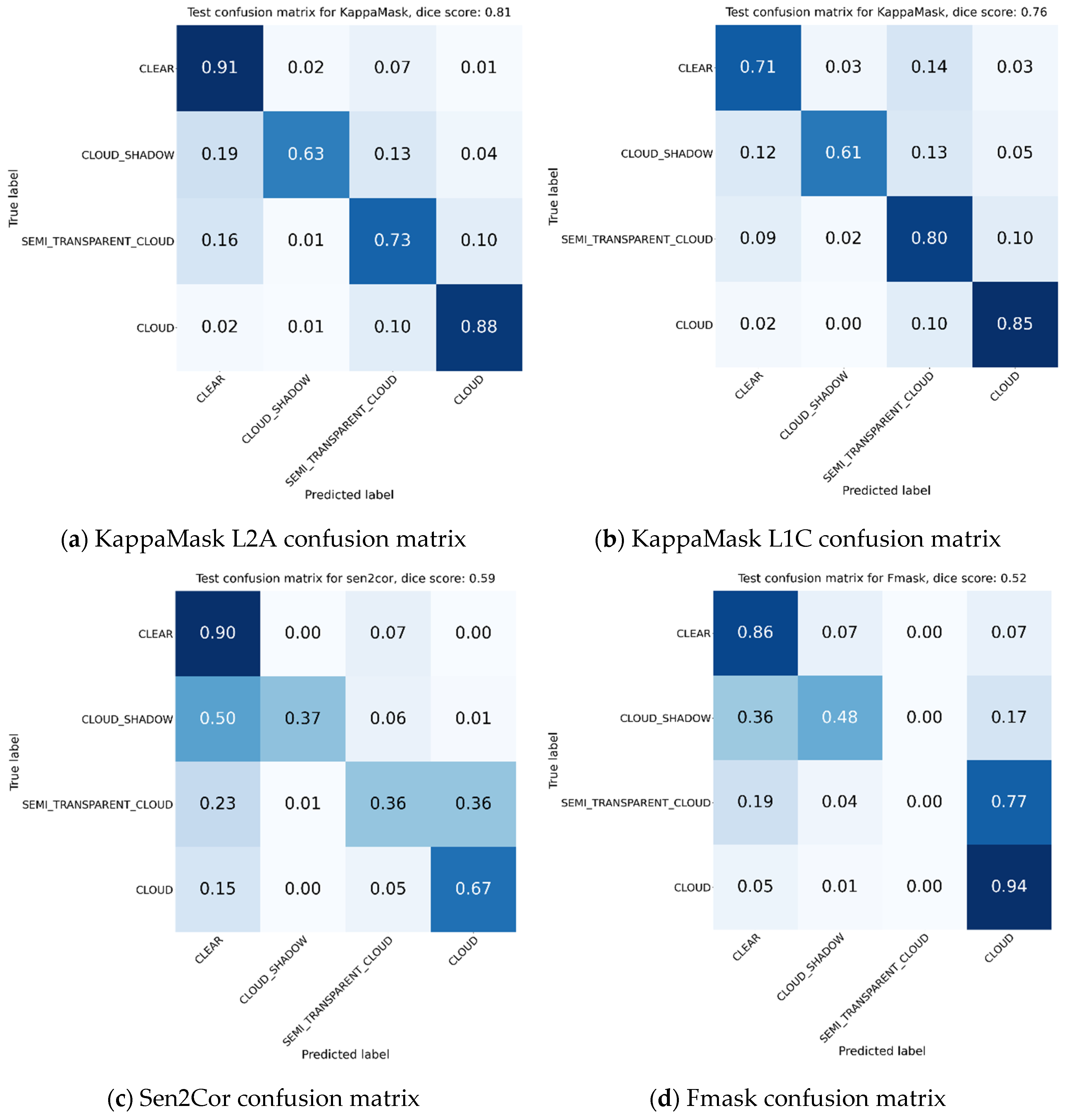
Figure 8.
Confusion matrices on test set for (a) KappaMask Level-2A; (b) KappaMask Level-1C; (c) Sen2Cor; (d) Fmask. Confusion matrix consists of clear, cloud shadow, semi-transparent cloud, cloud and missing class; however, the last one is removed from this comparison to make matrices easier to read.
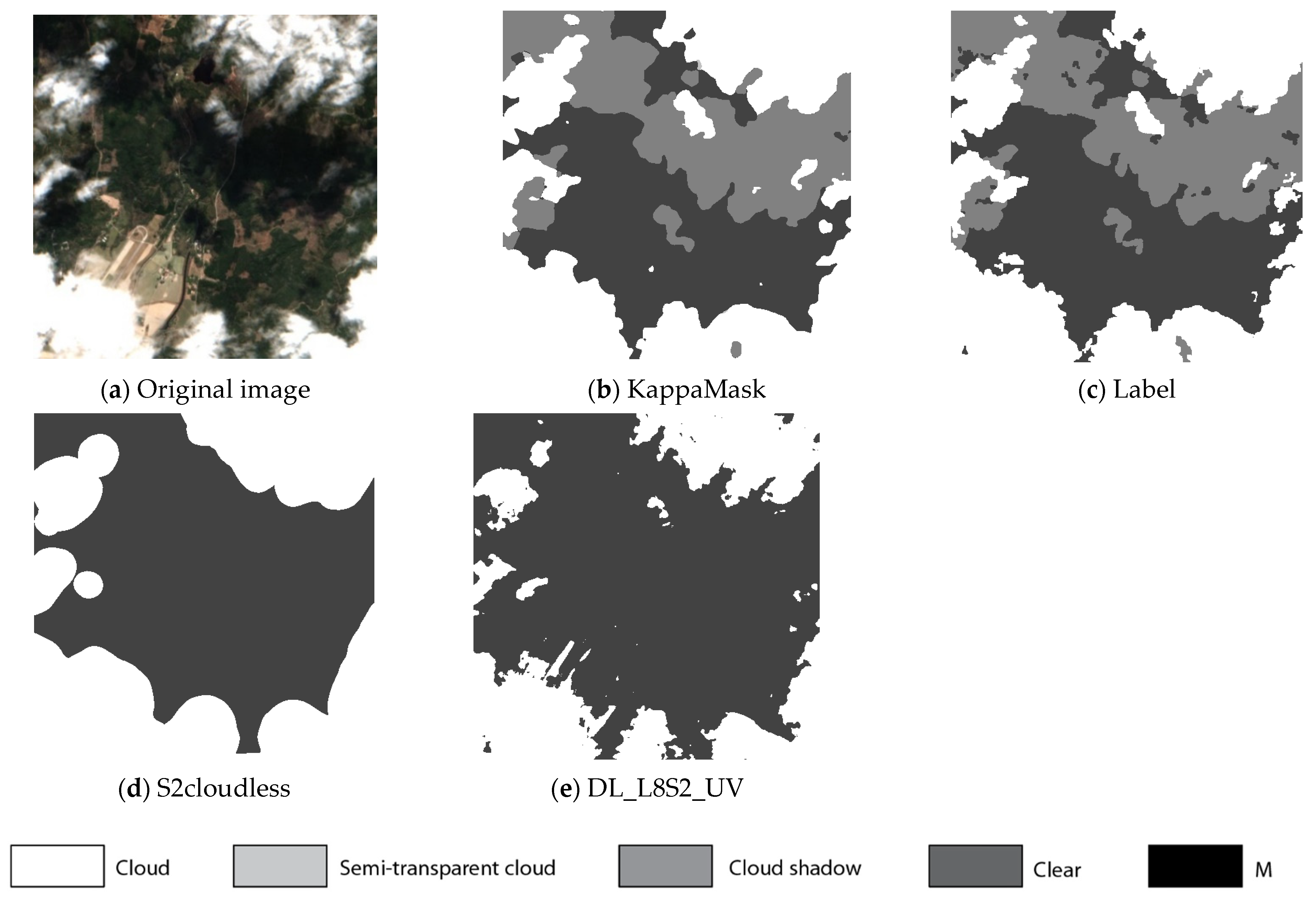
Figure 9.
Comparison of L2A prediction output for a 512 × 512 pixels sub-tile in the test dataset. (a) Original Sentinel-2 L2A True-Colour Image; (b) KappaMask classification map; (c) Segmentation mask prepared by a human labeller; (d) S2cloudless classification map; (e) DL_L8S2_UV classification map.
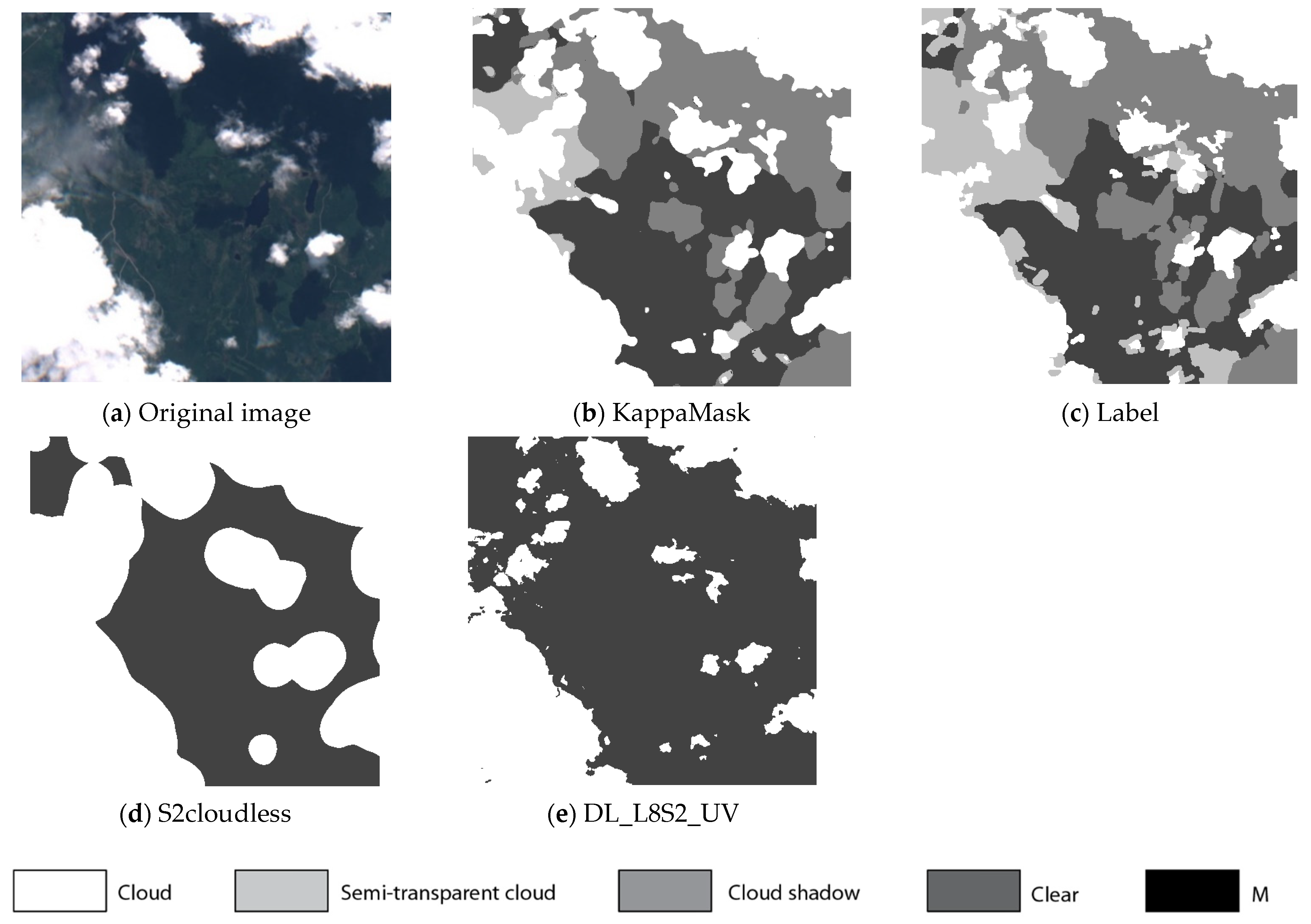
Figure 10.
Comparison of L1C prediction output for a 512 × 512 pixels sub-tile in the test dataset. (a) Original Sentinel-2 L1C True-Colour Image; (b) KappaMask classification map; (c) Segmentation mask prepared by a human labeller; (d) S2cloudless classification map; (e) DL_L8S2_UV classification map.
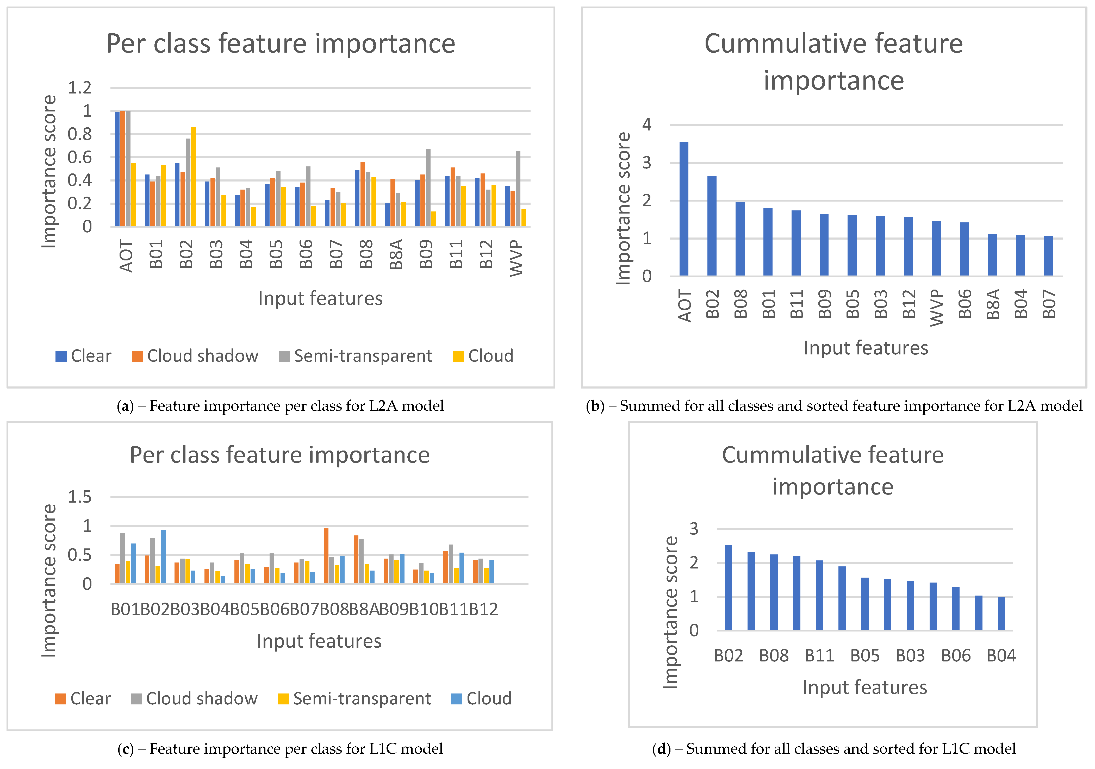
Figure 11.
Feature importance obtained by deleting input features during inference for L2A model: (a) feature importance per class; (b) sorted feature importance, summed up for all the classes, and for L1C model: (c) feature importance per class; (d) sorted feature importance, summed up for all the classes.
Table 1.
Output correspondence for different cloud classification masks. KappaMask output scheme is used for model fitting with logic corresponded to CMIX notation. Sen2Cor, Fmask, MAJA and S2cloudless are mapped respectively to KappaMask output. FMSC to Francis, Mrziglod and Sidiropoulos’ classification map [
27] is used for pretraining.
| Sen2Cor | CMIX | KappaMask | Fmask | S2Cloudless | FMSC |
|---|
| 0 No data | | 0 Missing | | | |
| 1 Saturated or defective | | 0 Missing | | | |
| 2 Dark area pixels | | 1 Clear | | | |
| 3 Cloud shadows | 4 Cloud shadows | 2 Cloud shadows | 2 Cloud shadows | | 2 Cloud shadows |
| 4 Vegetation | 1 Clear | 1 Clear | 0 Clear | 0 Clear | 0 Clear |
| 5 Not vegetated | | 1 Clear | | | |
| 6 Water | | 1 Clear | 1 Water | | |
| 7 Unclassified | | 5 Undefined | | | |
| 8 Cloud medium probability | | 4 Cloud | | | |
| 9 Cloud high probability | 2 Cloud | 4 Cloud | 4 Cloud | 1 Cloud | 1 Cloud |
| 10 Thin cirrus | 3 Semi-transparent cloud | 3 Semi-transparent cloud | | | |
| 11 Snow | | 1 Clear | 3 Snow | | |
Table 2.
Dice coefficient evaluation performed on the test dataset for KappaMask Level-2A, KappaMask Level-1C, Sen2Cor, Fmask and MAJA cloud classification maps. Evaluation is performed for clear, cloud shadow, semi-transparent and cloud classes.
Table 2.
Dice coefficient evaluation performed on the test dataset for KappaMask Level-2A, KappaMask Level-1C, Sen2Cor, Fmask and MAJA cloud classification maps. Evaluation is performed for clear, cloud shadow, semi-transparent and cloud classes.
| Dice Coefficient | KappaMask L2A | KappaMask L1C | Sen2Cor | Fmask | MAJA |
|---|
| Clear | 82% | 75% | 72% | 75% | 56% |
| Cloud shadow | 72% | 69% | 52% | 49% | - |
| Semi-transparent | 78% | 75% | 49% | - | - |
| Cloud | 86% | 84% | 62% | 60% | 46% |
| All classes | 80% | 76% | 59% | 61% | 51% |
Table 3.
Precision evaluation performed on the test dataset for KappaMask Level-2A, KappaMask Level-1C, Sen2Cor, Fmask and MAJA cloud classification maps. Evaluation is performed for clear, cloud shadow, semi-transparent and cloud classes.
Table 3.
Precision evaluation performed on the test dataset for KappaMask Level-2A, KappaMask Level-1C, Sen2Cor, Fmask and MAJA cloud classification maps. Evaluation is performed for clear, cloud shadow, semi-transparent and cloud classes.
| Precision | KappaMask L2A | KappaMask L1C | Sen2Cor | Fmask | MAJA |
|---|
| Clear | 75% | 79% | 60% | 66% | 64% |
| Cloud shadow | 82% | 79% | 87% | 51% | - |
| Semi-transparent | 83% | 71% | 78% | - | - |
| Cloud | 85% | 83% | 57% | 44% | 35% |
| All classes | 81% | 78% | 71% | 54% | 50% |
Table 4.
Recall evaluation performed on the test dataset for KappaMask Level-2A, KappaMask Level-1C, Sen2Cor, Fmask and MAJA cloud classification maps. Evaluation is performed for clear, cloud shadow, semi-transparent and cloud classes.
Table 4.
Recall evaluation performed on the test dataset for KappaMask Level-2A, KappaMask Level-1C, Sen2Cor, Fmask and MAJA cloud classification maps. Evaluation is performed for clear, cloud shadow, semi-transparent and cloud classes.
| Recall | KappaMask L2A | KappaMask L1C | Sen2Cor | Fmask | MAJA |
|---|
| Clear | 91% | 71% | 90% | 86% | 50% |
| Cloud shadow | 64% | 61% | 37% | 48% | - |
| Semi-transparent | 74% | 80% | 36% | - | - |
| Cloud | 87% | 85% | 67% | 60% | 65% |
| All classes | 79% | 74% | 58% | 65% | 58% |
Table 5.
Overall accuracy evaluation performed on the test dataset for KappaMask Level-2A, KappaMask Level-1C, Sen2Cor, Fmask and MAJA cloud classification maps. Evaluation is performed for clear, cloud shadow, semi-transparent and cloud classes.
Table 5.
Overall accuracy evaluation performed on the test dataset for KappaMask Level-2A, KappaMask Level-1C, Sen2Cor, Fmask and MAJA cloud classification maps. Evaluation is performed for clear, cloud shadow, semi-transparent and cloud classes.
| Overall Accuracy | KappaMask L2A | KappaMask L1C | Sen2Cor | Fmask | MAJA |
|---|
| Clear | 89% | 86% | 81% | 84% | 79% |
| Cloud shadow | 96% | 95% | 95% | 92% | - |
| Semi-transparent | 85% | 79% | 72% | - | - |
| Cloud | 92% | 91% | 78% | 67% | 63% |
| All classes | 91% | 88% | 82% | 81% | 71% |
Table 6.
Dice coefficient evaluation performed on the test dataset for KappaMask Level-2A, KappaMask Level-1C, S2cloudless and DL_L8S2_UV cloud classification maps. Evaluation is performed for clear, cloud shadow, semi-transparent and cloud classes.
Table 6.
Dice coefficient evaluation performed on the test dataset for KappaMask Level-2A, KappaMask Level-1C, S2cloudless and DL_L8S2_UV cloud classification maps. Evaluation is performed for clear, cloud shadow, semi-transparent and cloud classes.
| Dice Coefficient | KappaMask L2A | KappaMask L1C | S2cloudless | DL_L8S2_UV |
|---|
| Clear | 82% | 75% | 69% | 56% |
| Cloud | 86% | 84% | 57% | 67% |
| All classes | 84% | 80% | 63% | 62% |
Table 7.
Dice coefficient evaluation performed on the test dataset for KappaMask Level-2A, KappaMask Level-1C, S2cloudless and DL_L8S2_UVcloud classification maps. Evaluation is performed for clear, cloud shadow, semi-transparent and cloud classes.
Table 7.
Dice coefficient evaluation performed on the test dataset for KappaMask Level-2A, KappaMask Level-1C, S2cloudless and DL_L8S2_UVcloud classification maps. Evaluation is performed for clear, cloud shadow, semi-transparent and cloud classes.
| Precision | KappaMask L2A | KappaMask L1C | S2cloudless | DL_L8S2_UV |
|---|
| Clear | 75% | 79% | 59% | 41% |
| Cloud | 85% | 83% | 41% | 59% |
| All classes | 81% | 76% | 50% | 50% |
Table 8.
Dice coefficient evaluation performed on the test dataset for KappaMask Level-2A, KappaMask Level-1C, S2cloudless and DL_L8S2_UVcloud classification maps. Evaluation is performed for clear, cloud shadow, semi-transparent and cloud classes.
Table 8.
Dice coefficient evaluation performed on the test dataset for KappaMask Level-2A, KappaMask Level-1C, S2cloudless and DL_L8S2_UVcloud classification maps. Evaluation is performed for clear, cloud shadow, semi-transparent and cloud classes.
| Recall | KappaMask L2A | KappaMask L1C | S2cloudless | DL_L8S2_UV |
|---|
| Clear | 91% | 71% | 84% | 90% |
| Cloud | 87% | 85% | 93% | 77% |
| All classes | 89% | 78% | 89% | 84% |
Table 9.
Dice coefficient evaluation performed on the test dataset for KappaMask Level-2A, KappaMask Level-1C, S2cloudless and DL_L8S2_UVcloud classification maps. Evaluation is performed for clear, cloud shadow, semi-transparent and cloud classes.
Table 9.
Dice coefficient evaluation performed on the test dataset for KappaMask Level-2A, KappaMask Level-1C, S2cloudless and DL_L8S2_UVcloud classification maps. Evaluation is performed for clear, cloud shadow, semi-transparent and cloud classes.
| Overall accuracy | KappaMask L2A | KappaMask L1C | S2cloudless | DL_L8S2_UV |
|---|
| Clear | 89% | 86% | 80% | 61% |
| Cloud | 92% | 91% | 62% | 79% |
| All classes | 91% | 89% | 71% | 73% |
Table 10.
Training experiments for different model architectures for the L2A model.
Table 10.
Training experiments for different model architectures for the L2A model.
| Architecture | U-Net Level of Depth | Number of Input Filters | Max Dice Coefficient on
Validation Set |
|---|
| U-Net | 5 | 32 | 83.9% |
| 64 | 84.0% |
| 128 | 84.1% |
| 6 | 32 | 80.7% |
| 64 | 80.8% |
| 128 | 82.9% |
| 7 | 32 | 75.1% |
| 64 | 83.1% |
| U-Net++ | 5 | 64 | 75.9% |
Table 11.
Time comparison performed on one whole Sentinel-2 Level-1C product inference. KappaMask Level-1C with GPU and CPU, Fmask, S2cloudless and DL_L8S2_UV on generating 10 m resolution classification mask.
Table 11.
Time comparison performed on one whole Sentinel-2 Level-1C product inference. KappaMask Level-1C with GPU and CPU, Fmask, S2cloudless and DL_L8S2_UV on generating 10 m resolution classification mask.
| | KappaMask on GPU | KappaMask on CPU | Fmask | S2cloudless | DL_L8S2_UV |
|---|
| Running time | 03:57 | 10:08 | 06:32 | 17:34 | 03:33 |


 ,
, 


