Abstract
Vegetation phenology dynamics have attracted worldwide attention due to its direct response to global climate change and the great influence on terrestrial carbon budgets and ecosystem productivity in the past several decades. However, most studies have focused on phenology investigation on natural vegetation, and only a few have explored phenology variation of cropland. In this study, taking the typical cropland in the Shandong province of China as the target, we analyzed the temporal pattern of the Normalized Difference Vegetation Index (NDVI) and phenology metrics (growing season start (SOS) and end (EOS)) derived from the Global Inventory Monitoring and Modeling System (GIMMS) 3-generation version 1 (1982–2015) and the Vegetation Index and Phenology (VIP) version 4 (1981–2016), and then investigated the influence of climate factors and Net Primary Production (NPP, only for EOS) on SOS/EOS. Results show a consistent seasonal profile and interannual variation trend of NDVI for the two products. Annual average NDVI has significantly increased since 1980s, and hugely augmentations of NDVI were detected from March to June for both NDVI products (p < 0.01), which indicates a consistent greening tendency of the study region. SOSs from both products are correlated well with the ground-observed wheat elongation and spike date and have significantly advanced since the 1980s, with almost the same changing rate (0.65/0.64 days yr-1, p < 0.01). EOS also exhibits an earlier but weak advancing trend. Due to the significant advance of SOS, the growing season duration has significantly lengthened. Spring precipitation has a relatively stronger influence on SOS than temperature and shortwave radiation, while a greater correlation coefficient was diagnosed between EOS and autumn temperature/shortwave radiation than precipitation/NDVI. Autumn NPP exhibits a nonlinear effect on EOS, which is first earlier and then later with the increase of autumn NPP. Overall, we highlight the similar capacity of the two NDVI products in characterizing the temporal patterns of cropland phenology.
1. Introduction
Plant phenology, the study of annually recurring plant growth and reproductive events timing, and their endogenous and exogenous drivers [1], is influenced by changes in environmental factors, such as temperature, precipitation, sunlight [2,3]. Therefore, it is always an important factor to indicate global climate change [4,5]. Phenological shifts can not only greatly influence terrestrial carbon budgets and ecosystem productivity by altering the duration of photosynthesis [6], but also regulate climate change by modulating the land–atmospheric carbon, water, and energy exchange and land surface albedo [7,8]. In the past several decades, vegetation phenology dynamics have attracted worldwide attention due to climate change research. However, most studies have focused on the phenological changes of natural vegetation, and only a few have explored the phenological trends of agricultural varieties [9]. As the cultivated land accounts for approximately 12% of the global land area, phenological changes in crops could also largely affect global terrestrial mass and energy exchange [10]. Additionally, most of the published studies on agriculture phenology were conducted on site scale based on discrete ground data [11]. A comprehensive analysis of the effects of environmental factors on cropland phenology at a regional scale is still needed. Figuring out to what extent climate affects the cropland phenology would be helpful for agriculture management and plant breeding, even in the situation of hugely human impacts.
Compared with ground-manual records, remote sensing data confer excellent advantages for regional-scale phenology analysis because of their spatiotemporal continuity and landscape and community viewpoints [12]. For phenology analysis under the background of global change, the time span of datasets is a critical factor to successfully capture more detailed temporal profiles, and thus long-sequence remote sensing data are needed. Vegetation index data generated from the Advanced Very High-Resolution Radiometer (AVHRR) instruments are usually the first choice, as it has been collected by the National Oceanic and Atmospheric Administration (NOAA) satellites to monitor the earth surface since 1979. For this reason, the Normalized Differential Vegetation Index (NDVI) time series (over 30 years) derived from reflectance observed by channels 1 and 2 of AVHRR as part of the Global Inventory Modeling and Mapping Studies (GIMMS) project is often employed to investigate land surface dynamics at global and regional scales [3,13,14]. This dataset contributed to important findings on global land surface changes, especially prior to 2000 when other remote sensing data sources were relatively scarce. However, after the more advanced Moderate Resolution Imaging Spectroradiometer (MODIS) was launched in 1999 onboard the Terra satellite, MODIS-derived NDVI data became a primary tool to track changes in the landscape over time. On the one hand, MODIS data collection uses on-orbit calibration. Thus, data quality is significantly improved compared to previous satellite sensor data. On the other hand, the visible light and near-infrared range of MODIS is narrower, which gives it greater advantages to describe vegetation information with less interference. More importantly, MODIS has a finer spatial resolution (0.25–1 km) than AVHRR (1.1 km), which enables it to carry out more elaborate land surface studies over small regions. One disadvantage of MODIS compared to AVHRR is the relatively short time span. Therefore, many studies have attempted to generate a longer, high-quality time series by connecting the two sensors using quasi-physically based approaches [15] or statistical correlation analysis [16].
The NDVI data included in the Vegetation Index and Phenology (VIP) global datasets is a good product of these efforts that uses surface reflectance data from the AVHRR N07, N09, N11, and N14 datasets (1981–1999) and MODIS surface reflectance data (2000–2016). The systematic gaps between the two sensors are filled by standardizing AVHRR to the same level as MODIS. In comparison, GIMMS NDVI data are comprised of data from the AVHRR/2 instrument (1981–2000) and the AVHRR/3 instrument (2000–2015). VIP data have a finer spatial and temporal resolution, while GIMMS data possess the advantage of consistent sensors and band combinations. Some studies have compared VIP and GIMMS, but there is still a lack of detailed analysis of their performances in depicting vegetation dynamics of cropland, especially for phenology analysis [17]. Therefore, it is necessary to compare the performances of the two long-sequence datasets in phenology analysis for global change research. In this study, taking typical cropland of China as the target, we analyzed the difference of the two NDVI data sources in describing seasonal and interannual profiles and extracting phenology metrics and their variation trends by comparing with ground observations. Finally, we investigated the climate and biotic factors influencing the land surface phenology dynamics of cropland by means of gridded climate datasets.
2. Materials and Methods
2.1. Study Region
This study focused on Shandong Province in China. The central part of the province is mountainous, and the eastern part is hilly. The average elevation is approximately 90 m. Shandong is in a temperate climate zone with 4 distinct seasons. Summers are hot and rainy, whereas winters are cold and dry. The average temperature range in January is −5 to 1 °C and 24 to 28 °C in July. Annual precipitation ranges from 550 to 950 mm, the vast majority of which occurs in summer due to the influence of the monsoon. The study area is a famous wheat-corn rotation agricultural base in China. Cropland pixels were identified according to the International Geosphere-Biosphere Program global land cover classification system in the study region (Figure 1) [18]. Built-up and natural vegetation areas were not considered in this study.
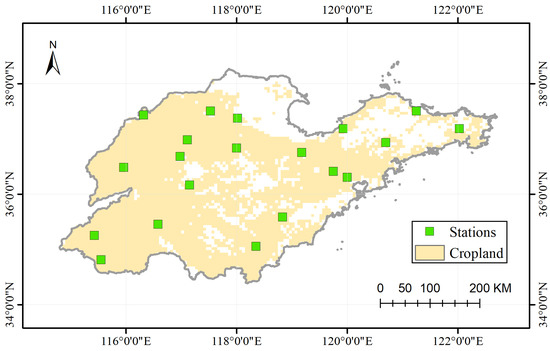
Figure 1.
Cropland and phenological stations distribution in Shandong Province of China. The distribution of cropland is identified according to the International Geosphere-Biosphere Program global land cover classification system.
2.2. Remote Sensing Data and Phenology Extraction
Two long-term NDVI datasets were used to extract vegetation phenology and compare their performances in phenological analysis. The first was the NDVI dataset (1981–2016) released by Vegetation Index and Phenology Laboratory at the University of Arizona (https://vip.arizona.edu/viplab_data_explorer.php, accessed on 15 December 2020). This dataset was created using surface reflectance data from the AVHRR N07, N09, N11, and N14 datasets (1981–1999) and MODIS Terra MOD09 surface reflectance data (2000–2016). The systematic gaps in NDVI values between the two sensors were filled through regression models by standardizing AVHRR to the same level as MODIS [16]. The current release is version 4 (hereafter called VIP for simplicity), and it has a spatial resolution of 0.05° and a temporal resolution of 7 days. The second product is the NDVI dataset from NOAA’s Global Inventory Monitoring and Modeling System (GIMMS 3g.v1) (https://data.tpdc.ac.cn/en/data/9775f2b4-7370-4e5e-a537-3482c9a83d88/, accessed on 15 December 2020). This long NDVI record is comprised of data from the AVHRR/2 instrument that spans from July 1981 to November 2000 and the AVHRR/3 instrument that continued these measurements from November 2000 to 2015 [19]. The current version is GIMMS 3g.v1 (hereafter called GIMMS for simplicity), which corrected drops in lower NDVI values after 2006 due to calibration and recovered negative NDVI values in winter for snow-covered regions of the Northern Hemisphere, compared to version 0. It has a twice-monthly temporal resolution, a spatial resolution of 1/12 degree, and spans from July 1981 to December 2015. Due to missing observations in the first half-year, NDVI spring phenology was not available. Therefore, we removed observations for 1981 from the whole NDVI sequence.
To guarantee the accuracy of phenology metrics extracted from the NDVI data, it was necessary to reconstruct high-quality NDVI time-series data by dealing with abnormal values [20]. Some abnormally low points may appear in the non-growing season due to the influence of snowfall, whereas a few abrupt and extreme low points may also exist in the middle of the growing season due to rainfall and clouds. For abnormal values in the non-growing season (defined as November-February according to local records), we used the average value of the top 50% higher NDVI values to replace the other 50% lower NDVI observations [21]. Then, the envelope line of the NDVI time series was obtained using a modified Savitzky–Golay filter [22], which simulates an ideal vegetation growth profile and removes the impacts of abrupt and extreme low values in the growing season. Finally, we fitted the reconstructed NDVI time series using a double logistic function, which performs well to model the vegetation growth process of the whole growing season [23,24]. Growing season start (SOS) and end (EOS) were obtained according to the locations of the maximum curvature of the fitted curve Equations (1)–(3).
where NDVI (t) is reconstructed NDVI values at time t; NDVImax and NDVImin are the maximum and minimum values in the NDVI time series, respectively; I and D represent the maximum rising and falling slopes (inflection points) on the fitted NDVI curve; S and E represent corresponding dates of I and D on the fitted NDVI curve. Growing season length (LOS) was defined as the duration from SOS to EOS. An illustration of phenology extraction can be found in Ren et al. [21]. To assess the fitted results, the mean squared error (MSE) between observed and predicted values was calculated for each pixel in each year [Equation (4)].
where ypre and yobs are the predicted and observed NDVI values, respectively; n denotes the NDVI sequence length. As no specific observation date was provided with the NDVI values in the GIMMS NDVI product, we simply took the middle date of each half-month as the ‘real’ date. For some cropland pixels with 2 growing seasons, we only computed the starting date of the first growing season and the ending date of the second growing season. Additionally, pixels with an annual amplitude of NDVI less than 0.1 were ignored in this study. All data processing was conducted using Matlab software (Mathworks, Matlab R2019a).
2.3. Ground Phenology Records
To assess the accuracy of satellite-derived SOS/EOS in this study, three ground-measured agriculture phenophases (the elongation/spike date records of wheat and the maturity date records of corn (773 in total, 1991–2013)) from 20 stations in Shandong province were employed to compare with SOS and EOS, respectively. They were observed by agrometeorological professionals and provided by China Meteorological Data Service Center (http://data.cma.cn/en, accessed on 15 May 2018). The elongation date of wheat was defined as the day when the internodes at the base of the stem were elongated and about 1.5–2.0 cm above the ground; the spike date of wheat was identified as the day when the tip of the ear was exposed from the flag sheath; and the maturity date of corn was characterized as the day when more than 80% of the outer bracts of the plants turn yellow, the filaments dry, and the grains harden [25]. The observation period varied among different phenophases and stations (Table 1).

Table 1.
Basic information of phenology observation stations.
2.4. Statistical Analysis
First, this study compared the seasonal profile of the spatial and multiyear average NDVI at each observation date and the interannual variation trend of the annually/monthly spatial average NDVI between VIP and GIMMS. Second, we compared the SOS/EOS and their variation trends among the two NDVI datasets and the ground-observed phenology metrics through Pearson correlation coefficients and bias (the average of the absolute difference). To eliminate the effect of extreme values in phenology extraction, we used the average SOS/EOS of 3 × 3 pixels around the location of phenological stations. The variation trends of NDVI, SOS/EOS, and ground observations were all computed with the linear regression. When conducting the direct comparison between SOS/EOS from the two NDVI datasets, we upscaled the spatial resolution of SOS/EOS from the VIP and GIMMS to 0.5° × 0.5° with arithmetic average method. Third, we took the daily temperature, precipitation, and shortwave radiation data from the WATCH-Forcing-Data-ERA-Interim data product (https://rda.ucar.edu/datasets/ds314.2/, accessed on 15 April 2021 [26]) to analyze the separate influence of climate factors on SOS/EOS by means of partial correlation analysis in each pixel. It had a spatial resolution of 0.5° × 0.5° and time span of 1981–2014. When conducting partial correlation analysis, the partial correlation coefficient was calculated between the average SOS/EOS of the two datasets and spring (March–May)/autumn (September–November) variables (average temperature, total precipitation, mean shortwave radiation, and average NDVI (only for EOS)) in each pixel, with one as the independent variable and others as the controlling variables. Meanwhile, the possible biotic impact of Net Primary Productivity (NPP) on EOS was also investigated through simple correlation analysis, which was from MODIS data products (MOD08_M3 v6.1, 2001–2014) in Google Earth Engine. Here, the spatially total NPP was used. All statistical and drawing processes were conducted by combining with Matlab software (Mathworks, R2019a), R, and ArcGIS 10.5 (Esri Inc., West Redlands, CA, USA).
3. Results
3.1. Comparison of Seasonal Profiles and Interannual Variation Trends of NDVI
The seasonal profiles of multi-year-space average NDVI from VIP and GIMMS showed a similar temporal pattern (Figure 2a). Two clear vegetation cycles were detected with mid-June as the approximate dividing point. This is attributed to the biannual cropping system in the study area. The NDVI amplitude of VIP was much larger than that of GIMMS. NDVI values from GIMMS were higher in the non-growing season and the first growing season but lower in the peak of the second growing season than VIP. Trend analyses illustrated that the annual average NDVI has significantly increased since the 1980s for both NDVI products (p < 0.01), which indicates a greening tendency of the study region (Figure 2b). They were also correlated well with each other (p < 0.05), indicating a consistent interannual variability tendency. Moreover, huge increases in NDVI value were detected from March to June for both NDVI products (Figure 2c,d). However, an approximate degree of NDVI growth in October, December, and January was detected only for the GIMMS product.
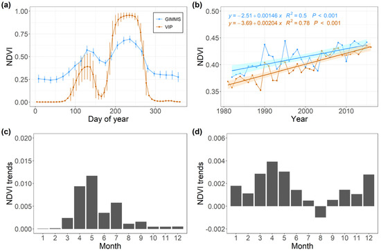
Figure 2.
Seasonal profiles and variation trends of the spatial average NDVI over the study region. (a) Seasonal profiles of the multi-year-space average NDVI from VIP (blue) and GIMMS (brown); (b) interannual changes of the spatial and annual average NDVI from VIP (blue) and GIMMS (brown); (c) monthly variation trend of NDVI for VIP; (d) monthly variation trend of NDVI for GIMMS. The error bar in (a) denotes the standard deviation.
3.2. Comparison of Phenology from Different Sources
Both the elongation and spike dates of wheat were used to compare with the SOS derived from VIP/GIMMS. As illustrated in Figure 3a–d, SOS exhibited a larger bias with the spike date (VIP: 25.9 days, GIMMS: 29.2 days) than the elongation date (VIP: 13.6 days, GIMMS: 13.4 days). They were correlated well with the two wheat phenophases (p < 0.01). In comparison, both EOSs from VIP (34.4 days) and GIMMS (24 days) were obviously later than the maturity date of corn (Figure 3e,f). No significant correlation was found for both and ground observations. When compared SOS/EOS between VIP and GIMMS, we identified that both SOS and EOS from VIP were averagely overestimated by about 16.7 and 12.1 days than that from GIMMS, respectively (Figure 4). However, they were correlated very well (p < 0.001), indicating a similar capacity to depict spatiotemporal patterns of the land surface.
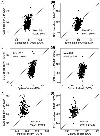
Figure 3.
Comparison of remotely based SOS/EOS and ground observations. (a)/(b) SOS derived from VIP/GIMMS vs. the elongation date of wheat; (c)/(d) SOS derived from VIP/GIMMS vs. the spike date of wheat; (e)/(f) EOS derived from VIP/GIMMS vs. the maturity date of corn. DOY means the day of the year.
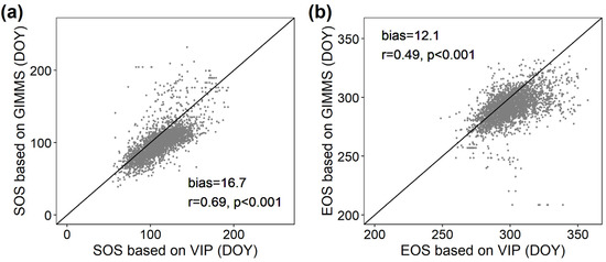
Figure 4.
Comparison of (a) SOS and (b) EOS derived from VIP and GIMMS. DOY means the day of the year.
3.3. Comparison of Phenological Trends from Different Sources
SOS retrieved from the two NDVI products has significantly advanced since the 1980s, with almost the same changing rate (0.65/0.64 days yr−1, p < 0.01) (Figure 5a). EOS derived from VIP also showed a significant advanced trend over time (0.2 days yr−1, p < 0.1) (Figure 5b). Consequently, LOS from both VIP and GIMMS exhibited a significant lengthening tendency, with the changing rate of 0.41 and 0.44 days yr−1, respectively (Figure 5c). However, a different variation trend was identified for the ground-observed phenophases. Both the elongation and spike date of wheat experienced a significant earlier trend (1.16 days yr−1 for the elongation, p < 0.05; 1.06 days yr−1 for the spike, p < 0.1) before 2002 but a significant delaying trend (0.84 days yr−1 for the elongation, p < 0.01; 1.04 days yr−1 for the spike, p < 0.01) after 2002 (Figure 5d,e). The maturity of corn has significantly delayed since the 1990s with a changing rate of 0.42 days yr−1 (p < 0.01) (Figure 5f).
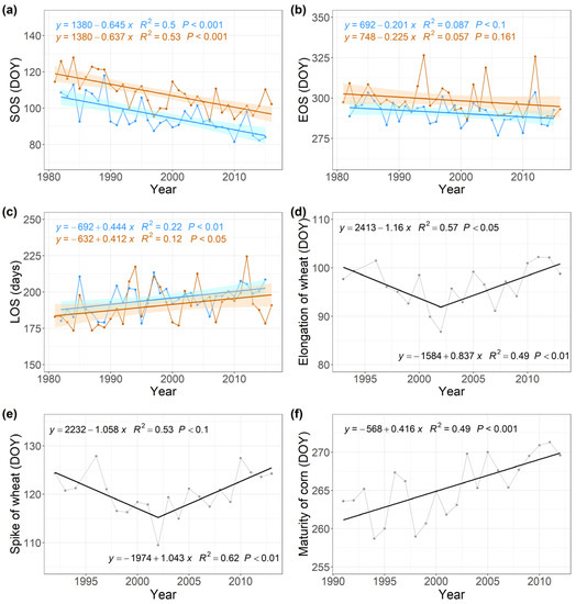
Figure 5.
Phenological trends comparison. (a) SOS, (b) EOS, and (c) LOS trends derived from VIP (blue) and GIMMS (brown) over the whole study region. (d–f) shows the variation trends of the elongation and spike date of wheat and the maturity date of corn, respectively. DOY means the day of year.
3.4. Influencing Factors Comparisons of SOS/EOS
By computing the partial correlation coefficients between SOS/EOS and spring/autumn temperature, precipitation, shortwave radiations, and annual mean NDVI (only for EOS), we found spring precipitation was a relatively stronger influence factor on SOS (−0.13 on average) compared with spring temperature (−0.03 in average) and shortwave radiation (0.07 in average) (Figure 6a). In comparison, a greater correlation coefficient was diagnosed between EOS and autumn average temperature (−0.22 on average)/shortwave radiation (0.26 on average) than that between EOS and autumn precipitation (0.15 on average)/NDVI (−0.07 in average) (Figure 6b). Increased autumn temperature/shortwave radiation would advance/delay the leaf senescence process. The positive correlations detected between EOS and autumn precipitation indicated a postponing effect of precipitation on the autumn phenology of crops. NDVI did not show obvious impacts on EOS, whereas the autumn NPP exhibited a nonlinear effect on EOS, namely first earlier and then later with the increase of autumn NPP (Figure 6c).
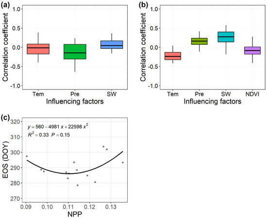
Figure 6.
Correlation coefficients between (a) SOS and spring average temperature (‘Tem’), total precipitation (‘Pre’), and mean shortwave radiation (‘SW’), and between (b) EOS and autumn average temperature, total precipitation, mean shortwave radiation, and NDVI. (c) Correlation between EOS and autumn total NPP.
4. Discussion
This study primarily analyzed the temporal patterns of NDVI and phenology metrics derived from two long-term NDVI datasets (VIP and GIMMS) for cropland in a typical cultivated region of China. First, a greening trend after the 1980s was observed for both datasets by calculating their variability over time. This is consistent with substantial land surface greening trends observed over the past few decades at the global scale, which may have resulted from enhanced photosynthesis driven by a warming climate and increasing CO2 concentrations [27,28,29]. Land-use change may also be an important explanation for the greening trend in some regions [30,31,32]. Unlike the present study, a clear inflection point of the greening trend was also found in the eastern part of the Tibetan Plateau, which may be due to the different vegetation types and altitudes [33]. Seasonally, both datasets showed a comparable number of growing cycles in most regions but with diverse amplitudes. For VIP, most NDVI values were around 0 in the non-growing season but close to 1 in the peak of the growing season. By comparison, the value of background NDVI for GIMMS was always near 0.2, and the higher NDVI was no more than 0.7 in most of the pixels. Except for the systematic difference of the two sensors in band passes, the continuity algorithm used for NDVI data generation could also further alter the NDVI profile magnitude when standardizing AVHRR to MODIS [16]. Nevertheless, the two datasets were largely consistent in capturing the seasonal and long-term pattern of growth status of local vegetation.
When used for vegetation phenology extraction, the two datasets showed a very close MSE in fitting NDVI time series (Figure 7), meaning almost equal fitting performance. Upon direct comparison, SOS/EOS based on the VIP dataset was found to be a little earlier by about two weeks than the values based on the GIMMS dataset, which indicates a little overestimation of SOS/EOS from VIP than GIMMS. However, when compared to the ground observed records, SOS from the two data sources presented a similar bias and correlation with them for spring phenology prediction, while EOS from GIMMS data seems to have a relatively small bias with the ground-observed maturity of corn than that from VIP. As to the variation trends of SOS/EOS for the two datasets, a consistent spatiotemporal pattern and interannual variability were observed. That means that both datasets could effectively describe the spatial and temporal traits of terrestrial ecosystems and reflect the impacts of regional climate change. The advanced SOS is also in accordance with previous results from the same data but different methods [3,34] and some ground-based manual observations [35,36]. However, differently, the elongation and spike date of wheat shows two segmented and opposite variation trends in this study. As to the variation trend of EOS, we detected a weak/non-significant advancing trend for GIMMS/VIP, which is different from the significant delaying trend found for ground observations and in other studies based on remote sensing data [37]. Consequently, a significant elongation of the growing season was identified for both, which is mainly resulted from the significant advance of SOS. Considering the relatively large bias of EOS identification, we think the accuracy of EOS may not be as high as SOS, which itself is more complicated than the spring phenology process and is easily affected by more elements, including abiotic and biotic factors [12]. Meanwhile, the mismatch of temporal patterns of phenology metrics from remote sensing data and ground observations may also be attributed to the noise information from other crops or natural vegetation included in the coarse remote sensing pixels [38]. Although the study region is a typical wheat-corn rotation planting area, other crops (such as vegetables, soybean, cotton, etc.) and natural vegetation are still unavoidable to exist sparsely around wheat/corn planting fields. In addition, different methods used for land surface phenology extraction can produce distinct or even opposite results for the same study region and period, which may also contribute a lot to the mismatch of temporal phenology pattern [39].
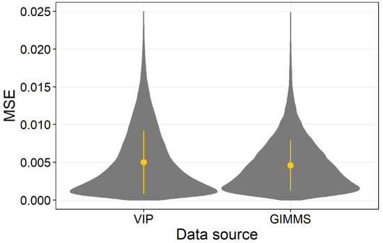
Figure 7.
Comparison of the average residual sum of squares (MSE) of the fitted NDVI time series between VIP and GIMMS.
Spring precipitation showed a relatively stronger influence on SOS than spring temperature and shortwave radiation, and more water availability would facilitate crops to grow earlier. Shandong province is a typical well-irrigated agriculture area in China. Nevertheless, spring drought often occurs in this region due to insufficient water storage in the soil and lack of precipitation [40]. Consequently, water supply serves as a critical factor limiting local crop growth. In comparison, the temperature did not exert a significant effect on SOS in our study region, which may be induced by the introduction of new and different cultivars with stronger tolerance of temperature changes over the study region. No obvious impacts of the shortwave radiation were found for SOS. This is different from the dominated temperature control found for spring phenology of wheat at a global scale [34]. Regarding to the influence of climate factors on EOS, we detected a negative effect of autumn temperature but a positive effect on autumn precipitation and shortwave radiation. Higher temperatures would speed up the heat accumulation needed for crops to mature and thus shorten the duration of the growth process. More precipitation and light availability can retard abscisic acid accumulation, enhance the chlorophyll levels, and thus slow the speed of leaf senescence [13]. In addition, we detected a two opposite-direction variation of EOS with the increase of NPP. In the first stage, augmented NPP causes an earlier EOS, as the excess of carbohydrates could lead to a downregulation of the photosynthetic genes and accelerate the induction of leaf senescence [41,42,43]. However, with the continuous growth of NPP, the excessive carbohydrates accumulation may take a longer time to be decomposed and consequently, in turn, postpone the growth cessation stage.
Overall, this study strengthens the relatively spatiotemporal consistency of phenology metrics retrieved from two long-term NDVI datasets. However, several points still need to be noted, which may cause some uncertainties to the results of this study. First, our study region only included the cropland and covered a small part of the agricultural region in China, and thus some results and conclusions may be somewhat biased. We expect to investigate larger regions and include other vegetation types in future research. Second, the mixed-pixel effect may have substantial effects on the results. The two NDVI datasets used in this study have relative coarser-resolution compared to the complicated planting strategies in the study region, where other crops (such as cotton, vegetables, soybeans, etc.) and natural vegetations are often sparsely distributed but possibly and totally account for a large part of a pixel (even greater than 50% for some special areas). They commonly have a large difference in the growth process. Therefore, a much finer land cover classification system and remote sensing data should be taken to conduct a more elaborate analysis. Third, although two NDVI datasets have a similar temporal pattern for NDVI and vegetation phenology, the gaps between them may not be ignored and should be considered when assessing physiological and ecological parameters, such as plant biomass [44], vegetation productivity [45], grain yields [46], etc. It may lead to greater errors due to land surface process estimation. Four, except for natural factors, crop growth progress is unavoidable to be influenced by human decision-making, such as sowing earlier or later, the choice of varieties, and the introduction of new cultivars [47,48,49], which need to be introduced in the following studies.
Author Contributions
Conceptualization, formal analysis, and writing, S.R.; validation and writing—review and editing, S.A. All authors have read and agreed to the published version of the manuscript.
Funding
This work was supported by the Shandong Provincial Natural Science Foundation (No. ZR2020QD001) of China.
Data Availability Statement
All data employed in this study are publicly and freely available. The NDVI dataset released by Vegetation Index and Phenology Laboratory could be downloaded at https://vip.arizona.edu/viplab_data_explorer.php. The Global Inventory Monitoring and Modeling System (GIMMS 3g.v1) NDVI data could be obtained from https://data.tpdc.ac.cn/en/data/9775f2b4-7370-4e5e-a537-3482c9a83d88/. Net Primary Productivity (NPP) data products (MOD08_M3 v6.1, 2001–2014) is available in Google Earth Engine. We are also sincerely grateful to the professionals working on ground-based observations and records.
Conflicts of Interest
The authors declare no conflict of interest.
References
- Chen, X. Plant Phenology of Natural Landscape Dynamics; Springer: Berlin/Heidelberg, Germany, 2017. [Google Scholar]
- An, S.; Chen, X.Q.; Zhang, X.Y.; Lang, W.G.; Ren, S.L.; Xu, L. Precipitation and Minimum Temperature are Primary Climatic Controls of Alpine Grassland Autumn Phenology on the Qinghai-Tibet Plateau. Remote Sens. 2020, 12, 431. [Google Scholar] [CrossRef]
- Liu, Q.; Fu, Y.H.; Zeng, Z.; Huang, M.; Li, X.; Piao, S. Temperature, precipitation, and insolation effects on autumn vegetation phenology in temperate China. Glob. Chang. Biol. 2016, 22, 644–655. [Google Scholar] [CrossRef] [PubMed]
- Kwembeya, E.G. Tracking biological footprints of climate change using flowering phenology of the geophytes: Pancratium tenuifolium and Scadoxus multiflorus. Int. J. Biometeorol. 2021, 65, 577–586. [Google Scholar] [CrossRef] [PubMed]
- Menzel, A.; Yuan, Y.; Matiu, M.; Sparks, T.; Scheifinger, H.; Gehrig, R.; Estrella, N. Climate change fingerprints in recent European plant phenology. Glob. Chang. Biol. 2020, 26, 2599–2612. [Google Scholar] [CrossRef] [PubMed]
- Richardson, A.D.; Keenan, T.F.; Migliavacca, M.; Ryu, Y.; Sonnentag, O.; Toomey, M. Climate change, phenology, and phenological control of vegetation feedbacks to the climate system. Agric. For. Meteorol. 2013, 169, 156–173. [Google Scholar] [CrossRef]
- Jeong, S.J.; Ho, C.H.; Kim, K.Y.; Jeong, J.H. Reduction of spring warming over East Asia associated with vegetation feedback. Geophys. Res. Lett. 2009, 36, L18705. [Google Scholar] [CrossRef]
- Liu, F.; Chen, Y.; Shi, W.; Zhang, S.; Tao, F.; Ge, Q. Influences of agricultural phenology dynamic on land surface biophysical process and climate feedback. J. Geogr. Sci. 2017, 27, 1085–1099. [Google Scholar] [CrossRef]
- Siebert, S.; Ewert, F. Spatio-temporal patterns of phenological development in Germany in relation to temperature and day length. Agric. For. Meteorol. 2012, 152, 44–57. [Google Scholar] [CrossRef]
- Asseng, S.; Ewert, F.; Martre, P.; Rötter, R.P.; Lobell, D.; Cammarano, D.; Kimball, B.; Ottman, M.; Wall, G.; White, J.W. Rising temperatures reduce global wheat production. Nat. Clim. Chang. 2015, 5, 143–147. [Google Scholar] [CrossRef]
- Tao, F.; Zhang, S.; Zhang, Z. Spatiotemporal changes of wheat phenology in China under the effects of temperature, day length and cultivar thermal characteristics. Eur. J. Agron. 2012, 43, 201–212. [Google Scholar] [CrossRef]
- Piao, S.; Liu, Q.; Chen, A.; Janssens, I.A.; Fu, Y.; Dai, J.; Liu, L.; Lian, X.; Shen, M.; Zhu, X. Plant phenology and global climate change: Current progresses and challenges. Glob. Chang. Biol. 2019, 25, 1922–1940. [Google Scholar] [CrossRef]
- Gao, M.; Wang, X.; Meng, F.; Liu, Q.; Li, X.; Zhang, Y.; Piao, S. Three-dimensional change in temperature sensitivity of northern vegetation phenology. Glob. Chang. Biol. 2020, 26, 5189–5201. [Google Scholar] [CrossRef]
- Ye, W.; van Dijk, A.I.; Huete, A.; Yebra, M. Global trends in vegetation seasonality in the GIMMS NDVI3g and their robustness. Int. J. Appl. Earth Obs. Geoinf. 2021, 94, 102238. [Google Scholar] [CrossRef]
- Steven, M.D.; Malthus, T.J.; Baret, F.; Xu, H.; Chopping, M.J. Intercalibration of vegetation indices from different sensor systems. Remote Sens. Environ. 2003, 88, 412–422. [Google Scholar] [CrossRef]
- Didan, K.; Barreto, A.; Miura, T.; Tsend-Ayush, J.; Zhang, X.; Friedl, M.; Gray, J.; Van Leeuwen, W.; Czapla-Myers, J.; Doman, B. Multi-Sensor Vegetation Index and Phenology Earth Science Data Records: Algorithm Theoretical Basis Document and User Guide Version 4.0; Vegetation Index and Phenology Lab, University of Arizona: Tucson, AZ, USA, 2015. [Google Scholar]
- Marshall, M.; Okuto, E.; Kang, Y.; Opiyo, E.; Ahmed, M. Global assessment of vegetation index and phenology lab (VIP) and global inventory modeling and mapping studies (GIMMS) version 3 products. Biogeosciences 2016, 13, 625–639. [Google Scholar] [CrossRef]
- Loveland, T.; Belward, A. The IGBP-DIS global 1km land cover data set, DISCover: First results. Int. J. Remote Sens. 1997, 18, 3289–3295. [Google Scholar] [CrossRef]
- Pinzon, J.E.; Tucker, C.J. A non-stationary 1981–2012 AVHRR NDVI3g time series. Remote Sens. 2014, 6, 6929–6960. [Google Scholar] [CrossRef]
- Zhang, X. Reconstruction of a complete global time series of daily vegetation index trajectory from long-term AVHRR data. Remote Sens. Environ. 2015, 156, 457–472. [Google Scholar] [CrossRef]
- Ren, S.L.; Chen, X.Q.; Lang, W.G.; Schwartz, M.D. Climatic Controls of the Spatial Patterns of Vegetation Phenology in Midlatitude Grasslands of the Northern Hemisphere. J. Geophys. Res. Biogeosci. 2018, 123, 2323–2336. [Google Scholar] [CrossRef]
- Chen, J.; Jönsson, P.; Tamura, M.; Gu, Z.; Matsushita, B.; Eklundh, L. A simple method for reconstructing a high-quality NDVI time-series data set based on the Savitzky–Golay filter. Remote Sens. Environ. 2004, 91, 332–344. [Google Scholar] [CrossRef]
- Atkinson, P.M.; Jeganathan, C.; Dash, J.; Atzberger, C. Inter-comparison of four models for smoothing satellite sensor time-series data to estimate vegetation phenology. Remote Sens. Environ. 2012, 123, 400–417. [Google Scholar] [CrossRef]
- Zhang, X.; Friedl, M.A.; Schaaf, C.B.; Strahler, A.H.; Hodges, J.C.F.; Gao, F.; Reed, B.C.; Huete, A. Monitoring vegetation phenology using MODIS. Remote Sens. Environ. 2003, 84, 471–475. [Google Scholar] [CrossRef]
- Administration, C.M. Observation Criterion of Agricultural Meteorology; China Meteorological Press: Beijing, China, 1993. [Google Scholar]
- Weedon, G.P.; Balsamo, G.; Bellouin, N.; Gomes, S.; Best, M.J.; Viterbo, P. The WFDEI meteorological forcing data set: WATCH Forcing Data methodology applied to ERA-Interim reanalysis data. Water Resour. Res. 2014, 50, 7505–7514. [Google Scholar] [CrossRef]
- Gao, X.; Liang, S.; He, B. Detected global agricultural greening from satellite data. Agric. For. Meteorol. 2019, 276, 107652. [Google Scholar] [CrossRef]
- Xue, Y.; Lu, H.; Guan, Y.; Tian, P.; Yao, T. Impact of thermal condition on vegetation feedback under greening trend of China. Sci. Total Environ. 2021, 785, 147380. [Google Scholar] [CrossRef]
- Zhu, Z.; Piao, S.; Myneni, R.B.; Huang, M.; Zeng, Z.; Canadell, J.G.; Ciais, P.; Sitch, S.; Friedlingstein, P.; Arneth, A. Greening of the Earth and its drivers. Nat. Clim. Chang. 2016, 6, 791–795. [Google Scholar] [CrossRef]
- Chen, C.; Park, T.; Wang, X.; Piao, S.; Xu, B.; Chaturvedi, R.K.; Fuchs, R.; Brovkin, V.; Ciais, P.; Fensholt, R. China and India lead in greening of the world through land-use management. Nat. Sustain. 2019, 2, 122–129. [Google Scholar] [CrossRef] [PubMed]
- Kolecka, N. Greening trends and their relationship with agricultural land abandonment across Poland. Remote Sens. Environ. 2021, 257, 112340. [Google Scholar] [CrossRef]
- Zhang, Y.; Song, C.; Band, L.E.; Sun, G.; Li, J. Reanalysis of global terrestrial vegetation trends from MODIS products: Browning or greening? Remote Sens. Environ. 2017, 191, 145–155. [Google Scholar] [CrossRef]
- Wang, H.; Peng, P.; Kong, X.; Zhang, T.; Yi, G. Vegetation dynamic analysis based on multisource remote sensing data in the east margin of the Qinghai-Tibet Plateau, China. PeerJ 2019, 7, e8223. [Google Scholar] [CrossRef]
- Ren, S.L.; Qin, Q.M.; Ren, H.Z. Contrasting wheat phenological responses to climate change in global scale. Sci. Total Environ. 2019, 665, 620–631. [Google Scholar] [CrossRef]
- Ge, Q.; Wang, H.; Dai, J. Phenological response to climate change in China: A meta-analysis. Glob. Chang. Biol. 2015, 21, 265–274. [Google Scholar] [CrossRef]
- Guo, L.; An, N.; Wang, K. Reconciling the discrepancy in ground-and satellite-observed trends in the spring phenology of winter wheat in China from 1993 to 2008. J. Geophys. Res. Atmos. 2016, 121, 1027–1042. [Google Scholar] [CrossRef]
- Luo, Z.; Yu, S. Spatiotemporal variability of land surface phenology in China from 2001–2014. Remote Sens. 2017, 9, 65. [Google Scholar] [CrossRef]
- Chen, X.; Wang, D.; Chen, J.; Wang, C.; Shen, M. The mixed pixel effect in land surface phenology: A simulation study. Remote Sens. Environ. 2018, 211, 338–344. [Google Scholar] [CrossRef]
- Ma, Y.; Liu, S. Time Series of Land Surface Phenology Dataset in Central Asia (1982–2015). J. Glob. Chang. Data Discov. 2020, 1, 31–37. [Google Scholar]
- Yu, H.; Zhang, Q.; Sun, P.; Song, C. Impact of droughts on winter wheat yield in different growth stages during 2001–2016 in Eastern China. Int. J. Disaster Risk Sci. 2018, 9, 376–391. [Google Scholar] [CrossRef]
- Paul, M.J.; Foyer, C.H. Sink regulation of photosynthesis. J. Exp. Bot. 2001, 52, 1383–1400. [Google Scholar] [CrossRef]
- Vitasse, Y.; Baumgarten, F.; Zohner, C.M.; Kaewthongrach, R.; Fu, Y.H.; Walde, M.G.; Moser, B. Impact of microclimatic conditions and resource availability on spring and autumn phenology of temperate tree seedlings. New Phytol. 2021, 232, 537–550. [Google Scholar] [CrossRef] [PubMed]
- Zani, D.; Crowther, T.W.; Mo, L.; Renner, S.S.; Zohner, C.M. Increased growing-season productivity drives earlier autumn leaf senescence in temperate trees. Science 2020, 370, 1066–1071. [Google Scholar] [CrossRef]
- Lumbierres, M.; Méndez, P.F.; Bustamante, J.; Soriguer, R.; Santamaría, L. Modeling biomass production in seasonal wetlands using MODIS NDVI land surface phenology. Remote Sens. 2017, 9, 392. [Google Scholar] [CrossRef]
- Erasmi, S.; Klinge, M.; Dulamsuren, C.; Schneider, F.; Hauck, M. Modelling the productivity of Siberian larch forests from Landsat NDVI time series in fragmented forest stands of the Mongolian forest-steppe. Environ. Monit. Assess 2021, 193, 1–18. [Google Scholar] [CrossRef]
- Mirasi, A.; Mahmoudi, A.; Navid, H.; Valizadeh Kamran, K.; Asoodar, M.A. Evaluation of sum-NDVI values to estimate wheat grain yields using multi-temporal Landsat OLI data. Geocarto Int. 2019, 36, 1–16. [Google Scholar] [CrossRef]
- He, L.; Asseng, S.; Zhao, G.; Wu, D.; Yang, X.; Zhuang, W.; Jin, N.; Yu, Q. Impacts of recent climate warming, cultivar changes, and crop management on winter wheat phenology across the Loess Plateau of China. Agric. For. Meteorol. 2015, 200, 135–143. [Google Scholar] [CrossRef]
- Liu, Y.J.; Chen, Q.M.; Ge, Q.S.; Dai, J.H.; Qin, Y.; Dai, L.; Zou, X.T.; Chen, J. Modelling the impacts of climate change and crop management on phenological trends of spring and winter wheat in China. Agric. For. Meteorol. 2018, 248, 518–526. [Google Scholar] [CrossRef]
- Wang, J.; Wang, E.; Feng, L.; Yin, H.; Yu, W. Phenological trends of winter wheat in response to varietal and temperature changes in the North China Plain. Field Crop. Res. 2013, 144, 135–144. [Google Scholar] [CrossRef]


Publisher’s Note: MDPI stays neutral with regard to jurisdictional claims in published maps and institutional affiliations. |
© 2021 by the authors. Licensee MDPI, Basel, Switzerland. This article is an open access article distributed under the terms and conditions of the Creative Commons Attribution (CC BY) license (https://creativecommons.org/licenses/by/4.0/).