1. Introduction
Knowledge of precipitation is critical to advancing our understanding of the water cycle and many other coupled (e.g., carbon, nitrogen) cycles of the Earth’s system. Reliable precipitation measurements and estimates are therefore vital for supporting and verifying climate, weather, and hydrological models, as well as the key components of other Earth system models. A wide range of instruments with varied coverage, resolution, and accuracy have been developed to measure precipitation. Compared with ground-based sensors such as rain gauges and weather radar, satellites have unique advantages in monitoring precipitation at regional to global scales, particularly in data-sparse areas such as the ocean, mountainous regions, and developing countries.
A large number of geostationary (GEO) and low earth orbit (LEO) satellites have been launched for monitoring a wide range of hydrometeorological variables, including precipitation [
1,
2,
3]. Different from LEO satellites, GEO platforms can provide very a high sampling frequency with much more detailed information, as they constantly focus on the same region. One of the most recent examples is the Geostationary Operational Environmental Satellite-16 (GOES-16; formerly known as GOES-R), which is jointly operated by the National Aeronautics and Space Administration (NASA) and the National Oceanic and Atmospheric Administration (NOAA). This new-generation GEO satellite, which improves greatly upon its predecessors, can conduct rapid scans of the continental United States (CONUS) every 5 min and two selected mesoscale (nominally 1000 km × 1000 km) areas every minute [
4]. Such high-resolution observations can substantially benefit global QPE at finer time and space scales. Despite the high-resolution images from GEO satellites, they often carry infrared (IR) sensors that are generally limited in accuracy of estimating surface precipitation rates, due to the indirect relationship between IR signals and precipitation [
1,
4]. In contrast, passive microwave (PMW) sensors onboard LEO satellites can directly sense the water and/or ice content in the clouds, and enable more accurate precipitation estimates [
5,
6]. Therefore, IR and PMW measurements are often merged to produce global multi-satellite precipitation products with increased accuracy, coverage, and resolution [
3,
7,
8,
9].
The QPE product derived from GOES-16 is mainly based on the Advanced Baseline Imager (ABI), a state-of-the-art 16-band radiometer that can achieve a spatial resolution of ~2 km and a temporal resolution of 10 min using its IR channels. Following the “multi-satellite” rationale, the operational GOES-16 QPE product was created based on the Self-Calibrating Multivariate Precipitation Retrieval algorithm (SCaMPR; [
10]), which calibrates the ABI-observed IR data to the NOAA’s Climate Prediction Center (CPC)’s combined microwave (MWCOMB) precipitation estimates (see [
3,
5] for more details).
This GOES-16 QPE product has provided new opportunities for various near-real-time (10 min) and local-scale (~2 km) hydrometeorological applications such as flash floods forecasting and landslides warnings due to its high resolution and very short latency [
4]. Its accuracy, however, remains unclear due to the limited high-quality ground reference and comprehensive evaluation works. To address this critical problem, this study aims to provide a thorough assessment of the GOES-16 QPE product by leveraging the high-quality ground-based QPE from the MRMS system over CONUS. In particular, we selected the gauge-corrected MRMS (GC-MRMS) QPE product, which covers the entire CONUS with a spatial and temporal resolution of 1 km and 1 hour, respectively [
11]; it has been widely used as a ground reference in verifying satellite precipitation products (e.g., [
12,
13]).
Section 2 presents the study domain, data, and evaluation methodology. The cross-validation results, including the contingency tables and quantitative evaluation scores, are detailed in
Section 3.
Section 4 provides a thorough discussion of the performance of the GOES-16 QPE and the associated SCaMPR algorithm.
Section 5 concludes the study and suggests future research directions.
2. Materials and Methods
2.1. Study Domain
We selected CONUS as the study domain (
Figure 1; it lies between 20°–55°N latitude and 60°–130°W longitude) because it is characterized by a diverse climate and precipitation patterns, and is covered by a high-quality, high-resolution ground reference data GC-MRMS. However, the limited accuracy of radar observations over the western United States has been well recognized due to beam blockage in the mountainous Rockies [
11,
14]. For this reason, the study domain was further divided into two subdomains by simply using the 105°W longitude line: CONUS-east and CONUS-west.
Figure 1 shows the digital elevation model (DEM) map for CONUS and the division of the two subdomains (the thick black line represents the meridian 105°W).
2.2. Datasets
In this study, the SCaMPR-derived GOES-16 ABI L2+ QPE was verified against the MRMS product (GaugeCorr_QPE_01H) over the CONUS. The warm seasons (May to September) during 2018–2019 were selected as the study periods, mainly because precipitation during these periods was relatively abundant, and the MRMS product was less affected by ground clutter.
2.2.1. Ground Reference: MRMS
The ground reference precipitation dataset was obtained from the MRMS system, which combines about 160 polarimetric WSR-88D radars with rain gauges and other auxiliary environmental information to generate CONUS-wide, high-resolution QPE products and associated diagnostic products (e.g., precipitation type and radar quality index) [
14]. In this study, we used the hourly 0.01° (~1 km) GC-MRMS QPE product, which had integrated quality-controlled gauge observations to ensure the best data quality.
2.2.2. GOES-16 QPE Product
The operational GOES-16 QPE product provides precipitation at global scale with a spatial resolution of 0.02° (2 km; at the equator) and a temporal resolution of 10 min. It is derived based on the SCaMPR algorithm [
10,
15], which takes full advantage of the brightness temperature (TB) information from multiple ABI IR channels. Specifically, the SCaMPR algorithm consists of two major steps: the discriminant analysis for rainfall detection, and then stepwise forward linear regression for rain rates estimation at the identified rainy pixels. The ABI IR-retrieved raining area and rainfall intensity are further calibrated to the CPC’s MWCOMB precipitation estimates [
3]. The GOES-16 QPE data can be accessed at
https://www.ncdc.noaa.gov/airs-web/search?datasetid=ABIL2PROD, accessed on 1 June 2020.
2.3. Methodology
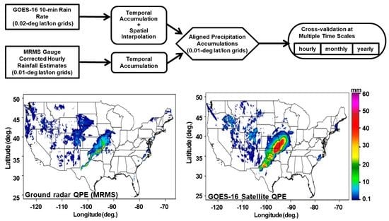
2.3.1. Space–Time Alignment
The GOES-16 QPE product and GC-MRMS vary in their spatial coverage, grid size, and temporal scale. First of all, the global GOES-16 QPE was clipped to the CONUS, and its 10-minute precipitation estimates were temporally aggregated into hourly totals to match the time scale of the GC-MRMS data. Then, the coarser (0.02°) GOES-16 QPE was spatially interpolated into the GC-MRMS grid (0.01°) using nearest-neighbor interpolation. Because different hydrometeorological applications for GOES-16 QPE are characterized by different time scales (e.g., flash flooding is often caused by short-lived heavy rainfall, while agricultural irrigation water is likely to be determined by monthly rainfall amount), we further accumulated the hourly precipitation estimates from GOES-16 QPE and GC-MRMS into daily and monthly scales for a comprehensive evaluation.
Figure 2 summarizes the above space–time alignment procedure, and
Figure 3 presents an example that compares the resampled hourly GOES-16 QPE with GC-MRMS over the CONUS for 0200–0300 UTC on 21 May 2019.
2.3.2. Evaluation Metrics
In the study, a rain/no-rain detection threshold of 0.1 mm/h (at a 10-minute resolution) was applied to the GOES-16 QPE. That is, only grid pixels with a precipitation rate higher than 0.1 mm/h were considered in the following evaluation analysis.
For the detection skills of the GOES-16 QPE, we used the probability of detection (
POD), false alarm rate (
FAR), and critical success index (
CSI). The Hedwig skill score (
HSS) was also computed to indicate the overall accuracy of the GOES-16 QPE product for capturing precipitation occurrence. These were defined as follows:
where
H is the number of pixels for which both GOES-16 QPE and GC-MRMS detected precipitation;
F is the number of false alarms (i.e., GOES-16 QPE identified precipitation, but GC-MRMS did not);
M is the number of missed precipitation pixels (i.e., GC-MRMS detected rainy pixels that were not captured by GOES-16 QPE); and
n is the number of correct non-precipitation grids from both. The detection skill improves as
POD increases from 0 to 1, while
FAR changes in the opposite direction. In theory, the perfect score for
CSI and
HSS is 1.
To quantitatively evaluate the performance of GOES-16 in estimating rain rates (when rain was detected), the mean error (
ME), normalized mean error (
NME), normalized mean absolute error (
NMAE), root-mean-square error (
RMSE), and Pearson’s correlation coefficient (
CC) were calculated, which were respectively defined as follows:
where
is the GC-MRMS estimated rainfall,
is the rainfall estimated by the GOES-16 QPE,
N is the total number of precipitation pixels, and <·> stands for the sample average.
Here, it should be noted that all Equations (1a)–(2e) used the GC-MRMS as references, and only the pairs of GOES-16 and GC-MRMS estimates in which the latter was greater than the rain/no-rain threshold (i.e., 0.1 mm, at all temporal scales used in this study) were used in computing the statistics in Equation (2a–e). For regional-scale analysis, the evaluation statistics were first calculated over each precipitation pixel where the GC-MRMS observed precipitation exceeded the threshold, and then the regionwide statistics were calculated by averaging over all precipitation pixels. In addition, the Probability Density Functions (PDF) of rainfall amounts for GOES-16 QPE and GC-MRMS were also compared at seasonal and monthly scales, to characterize the full distribution information retrieved by GOES-16 QPE.
2.3.3. Heavy Rain Events
To further evaluate the accuracy of precipitation estimated by the GOES-16 QPE, two featured heavy precipitation events were selected (i.e., 29 August 2018 and 8 May 2019) for a detailed comparison. The two events were considered because the peak rainfall intensity exceeded 15 mm/h, and both events were widespread. For this event-based analysis, evaluation scores were first computed at each hour during the event, and the differences in these scores between hourly rainfall accumulations were also investigated.
3. Results
3.1. Total Rainfall Accumulations
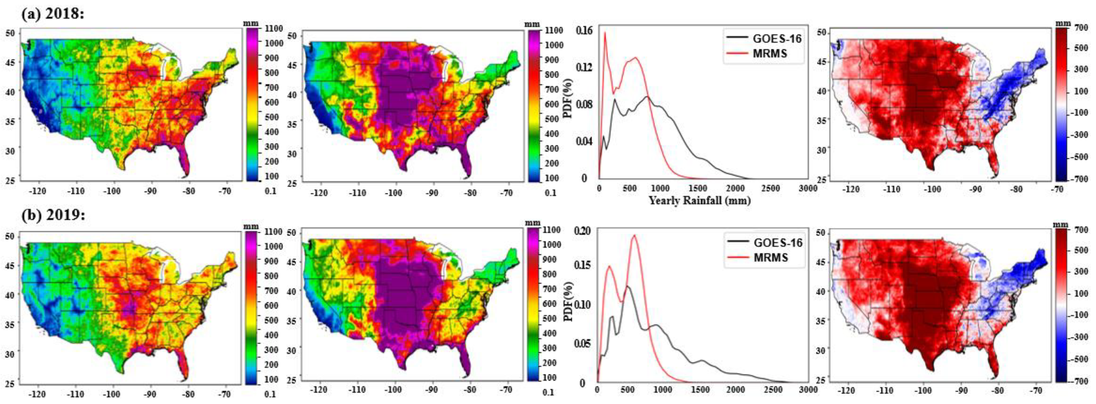
Figure 4 compares the warm-season total accumulations from GC-MRMS and GOES-16 QPE and their difference in 2018 and 2019. In terms of total precipitation amount, the GOES-16 QPE generally overestimated rainfall, particularly over the Great Plains (roughly between 90°W and 105°W), while it underestimated rainfall in the northeastern CONUS.
In addition, the PDF-based comparison of the GOES-16 QPE and GC-MRMS estimated warm-season total rainfall highlighted the magnitude-dependent performance of the GOES-16 QPE. In short, the GOES-16 QPE tended to underestimate warm-season total rainfall when it was below 800 mm, and to overestimate it for rainfall greater than 800 mm. In this regard, the PDF curves estimated by GOES-16 were shifted towards heavy rainfall.
Table 1 presents the evaluation statistics for GOES-16 estimated total rainfall amount during the warm season in 2018 and 2019, including the regional summary over CONUS-east, CONUS-west, and the entire CONUS, respectively. For CONUS-east (CONUS-west), the GOES-16 QPE overestimated warm-season rainfall totals by 340 (255) mm in 2018 and 433 (258) mm in 2019. The GOES-16 QPE was found to be highly correlated with the GC-MRMS reference over the CONUS (
CC was 0.59 (0.65) in 2018 (2019)). Meanwhile, this correlation obviously differed between CONUS-east and CONUS-west, which was primarily reflected by lower scores for CONUS-east and higher scores for CONUS-west. This was mainly due to the complex terrains in the CONUS-west, the uncertainty of which introduced more errors in precipitation detection by the ground network.
3.2. Monthly Rainfall
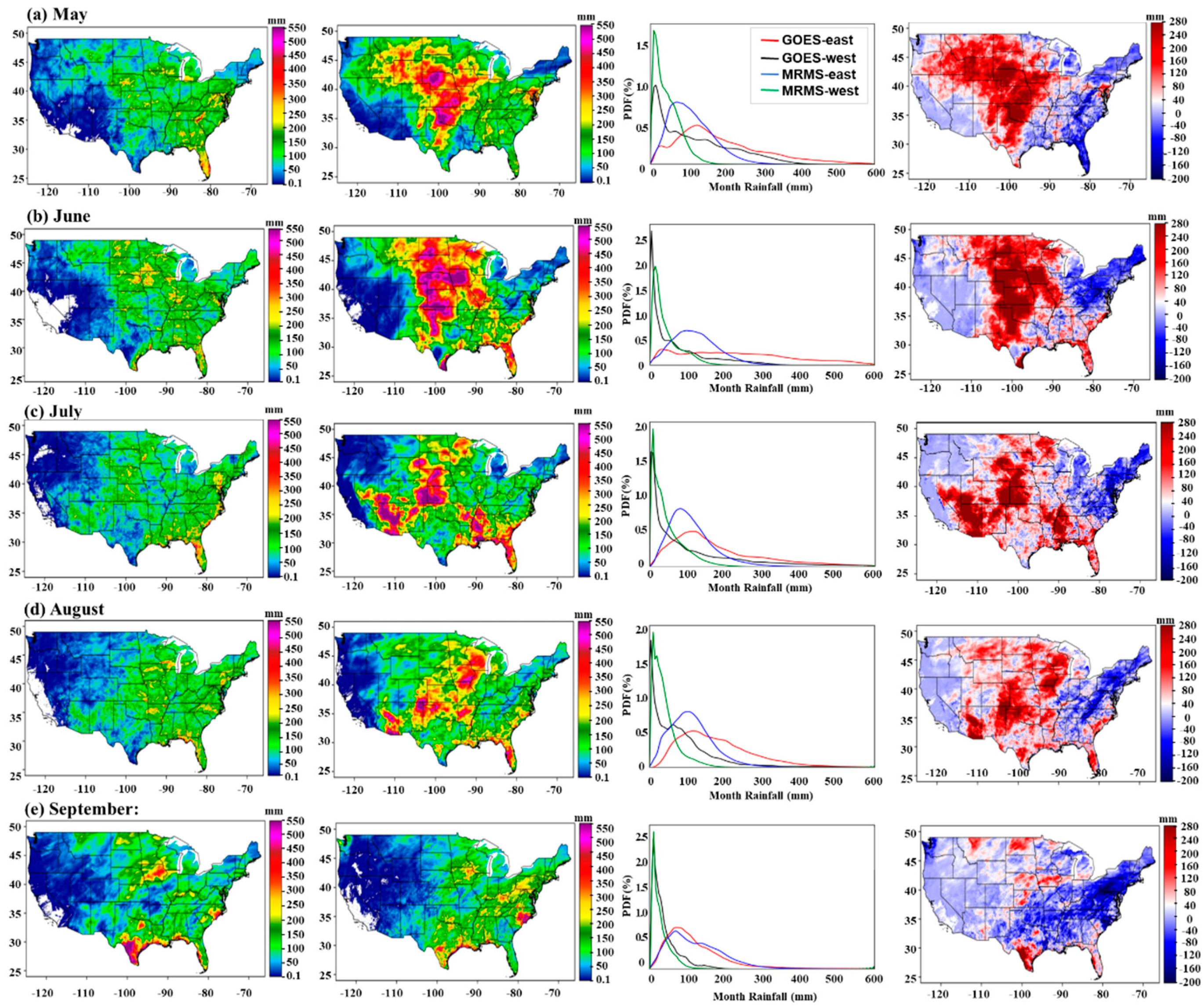
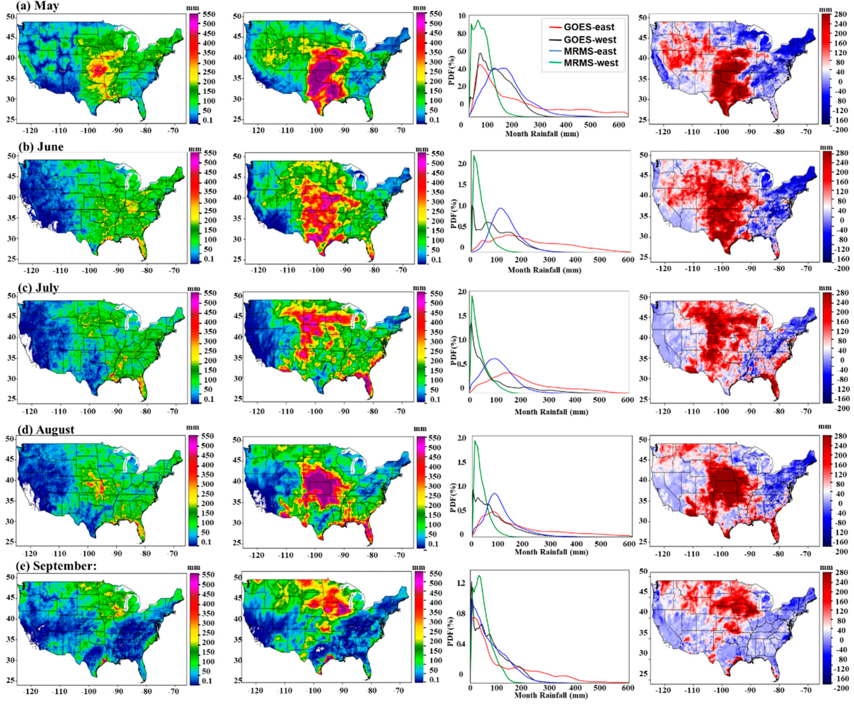
Figure 5 presents the comparison of the monthly rainfall maps derived from GOES-16 QPE and GC-MRMS in 2018, and
Figure 6 shows the same results for 2019. The results from May to September are shown from top to bottom. Similar to the seasonal results, the GOES-16 QPE overestimated precipitation over the central Great Plains, while underestimating it mainly in the northeastern CONUS. We further compared the difference between CONUS-east and CONUS-west in terms of the PDF curves for monthly rainfall. The monthly-scale PDF was obviously skewed, with more precipitation in the CONUS-east and less precipitation in the CONUS-west. In particular, the PDF of QPE from MRMS was higher than GOES-16 when precipitation values were under 160 mm on a monthly scale, while the PDF from the two QPEs showed the opposite results when precipitation values were higher than 160 mm.
Table 2 and
Table 3 summarize the monthly evaluation scores from May to September in 2018 and 2019 for CONUS-east and CONUS-west, respectively. Specifically for CONUS-east,
CC was 0.59 in September 2018, while
CC reached 0.80 in 2019, and exhibited a relatively stronger correlation. In terms of other evaluation scores, September was also the best over CONUS-east. In contrast,
CC fell to 0.51 (0.64) in September 2018 (2019) over CONUS-west. In general, the performances of the monthly GOES-16 QPE for CONUS-east and CONUS-west were similar.
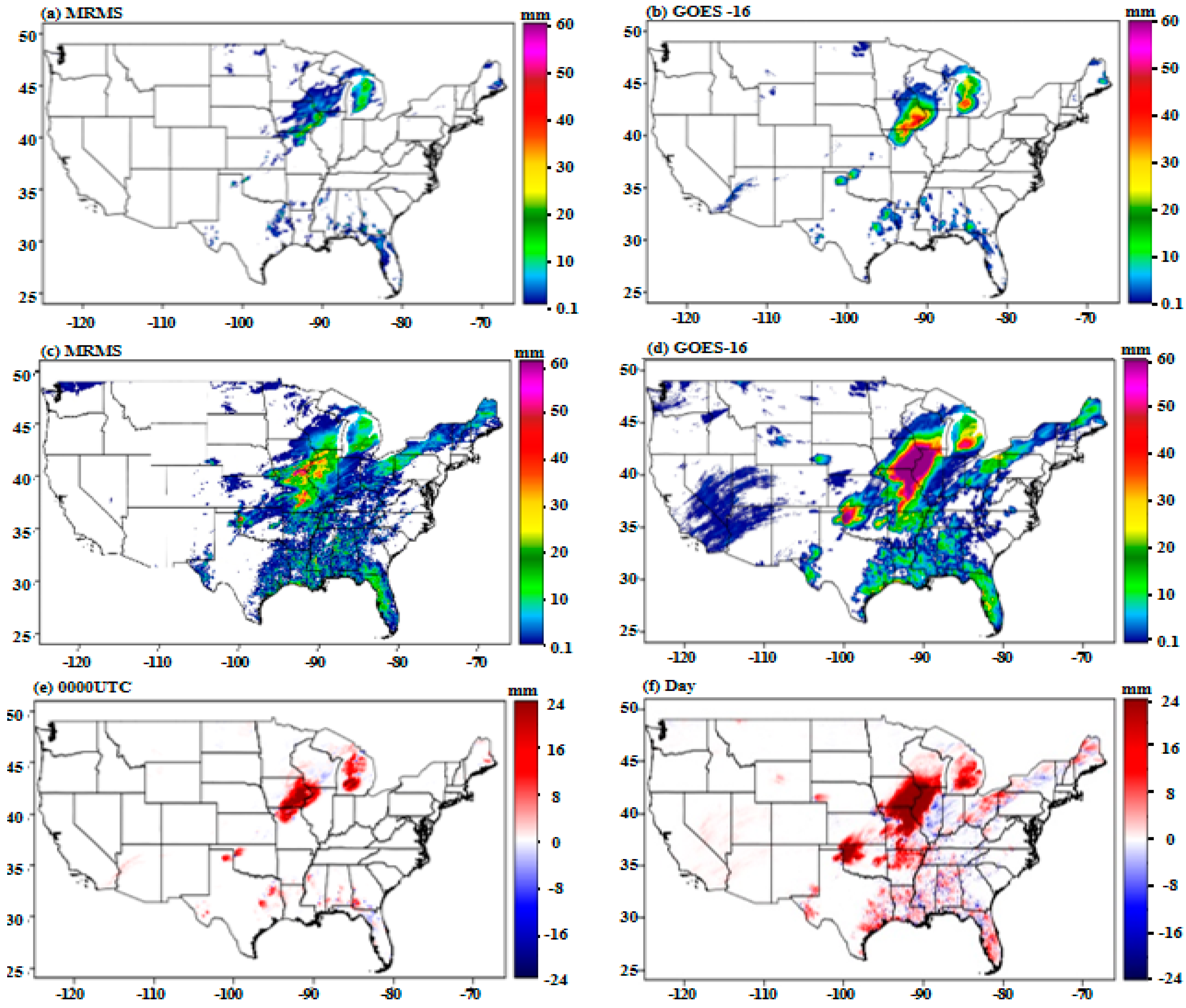
3.3. Daily Rainfall
Figure 7c,d,f show an example of the estimated daily precipitation between GC-MRMS and the GOES-16 QPE, and their difference on 8 May 2019. The spatial maps show that GOES-16 QPE also exhibited a noticeable regional difference compared to GC-MRMS at a daily scale.
The evaluation results for the GOES-16 QPE estimated daily precipitation are detailed in
Table 4 and
Table 5, showing the statistics month by month and over CONUS-east and CONUS-west, respectively. The last column represents the average over all the months. In CONUS-east, similar results were obtained in 2018 and 2019. According to the average,
CSI was approximately 0.6, due to relatively high
POD and low
FAR values. The
CC value was 0.47, and the
RMSE was around 18.00. In addition, the daily precipitation estimated by the GOES-16 QPE was higher than the GC-MRMS estimates every month. In contrast, in CONUS-west, the detection skills of the GOES-16 QPE decreased significantly, while the maximum
CC was also reduced to 0.33.
3.4. Hourly Precipitation
To fully characterize the retrieval skills of the GOES-16 QPE, the time scale for evaluation was further reduced to hourly, and the results are listed in
Table 6 and
Table 7 for CONUS-east and CONUS-west, respectively. The performance metrics were averaged in each month, and the whole season averaged results are also shown in the last column.
In summary, the average scores in 2018–2019 over CONUS-east were 9.16 (ME), 0.48 (NME), 0.96 (NMAE), 8.33 (RMSE), 0.30 (CC), 0.46 (POD), 0.27 (CSI), 0.58 (FAR), and 0.38 (HSS). For CONUS-east, the average POD was 0.46 and FAR was 0.58, indicating a good matching between the GOES-16 QPE and GC-MRMS for warm-season precipitation. For detected precipitation, the GOES-16 QPE estimated hourly precipitation accumulation was 0.48 mm/h lower than that of GC-MRMS.
By contrast, for CONUS-west, the average scores of hourly precipitation accumulation were 11.18 (ME), 0.7 (NME), 0.97 (NMAE), 7.05 (RMSE), 0.13 (CC), 0.32 (POD), 0.18 (CSI), 0.67 (FAR), and 0.26 (HSS). POD was decreased by only 0.32, while CC was only 0.13, with a significant weak correlation. Meanwhile, the GOES-16 QPE was 0.7 mm/h lower than GC-MRMS, demonstrating a dramatic difference compared to CONUS-east. These apparent regional differences indicated that GOES-16 provided poor evaluations for CONUS-west compared to CONUS-east, which was likely caused by the limitations of GOES-16 QPE’s retrieval algorithm over the complex terrains.
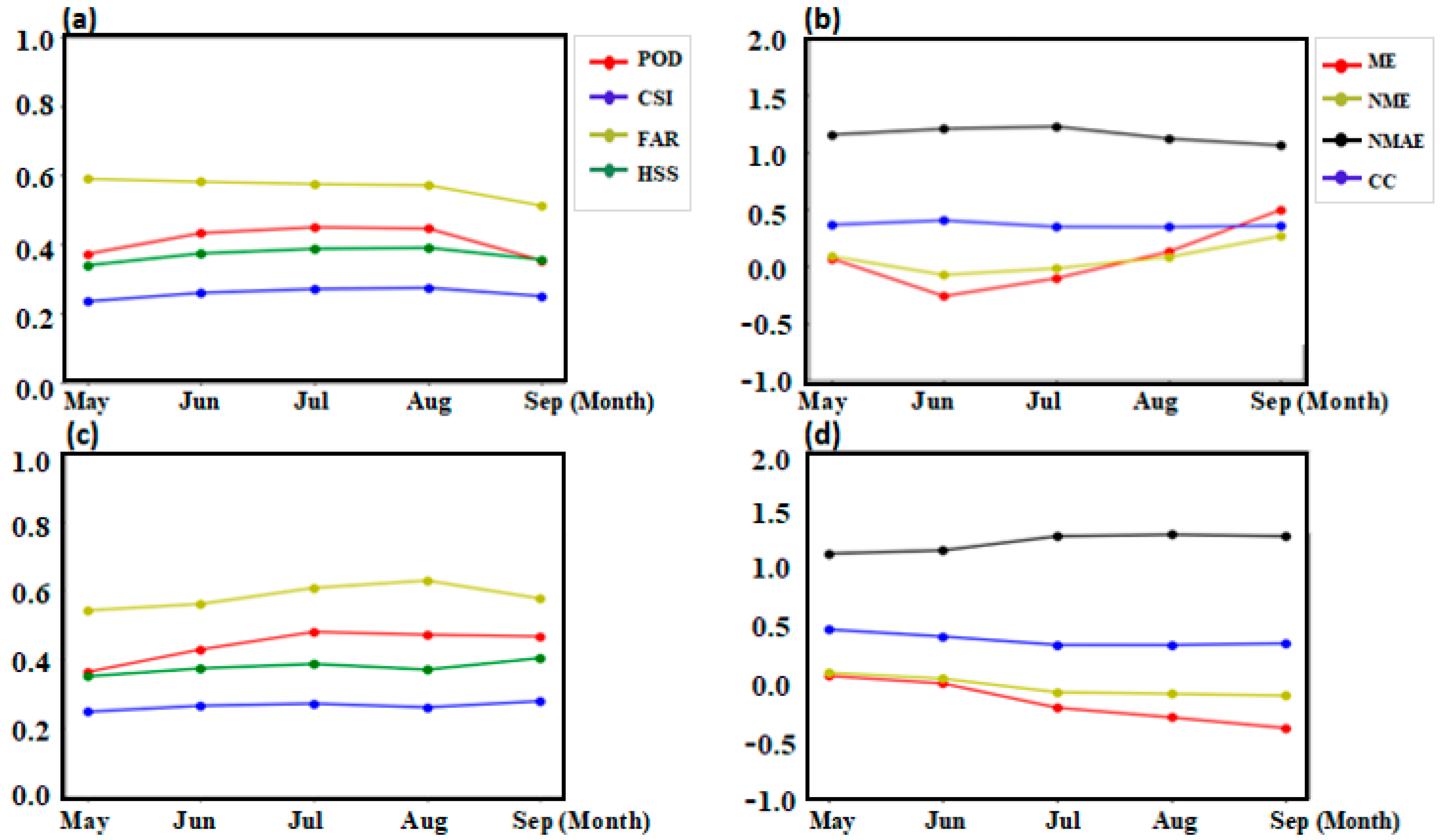
To explore the temporal variations in the GOES-16 QPE’s performance, the month-to-month changes in hourly evaluation statistics are shown in
Figure 8. For simplicity, only the results for CONUS-east are presented here. Compared to May–August,
CSI was 0.3 in September 2018 due to a significant increase in
POD;
FAR (0.5) decreased, and
HSS was 0.4 (from
Figure 8). In particular,
POD increased to 0.53 in September 2019, indicating that the precipitation algorithm performed well during a period with a high frequency of heavy precipitation. The scores for
ME,
NME,
NMAE, and
CC for hourly precipitation accumulation in 2018 and 2019 are shown in
Figure 8b,d, respectively.
NMAE was lowest in September 2018, with a value of approximately 1.0, and
NME was 0.4. These results indicated that the GOES-16 precipitation algorithm performed better for the months when heavy precipitation occurred frequently, such as September.
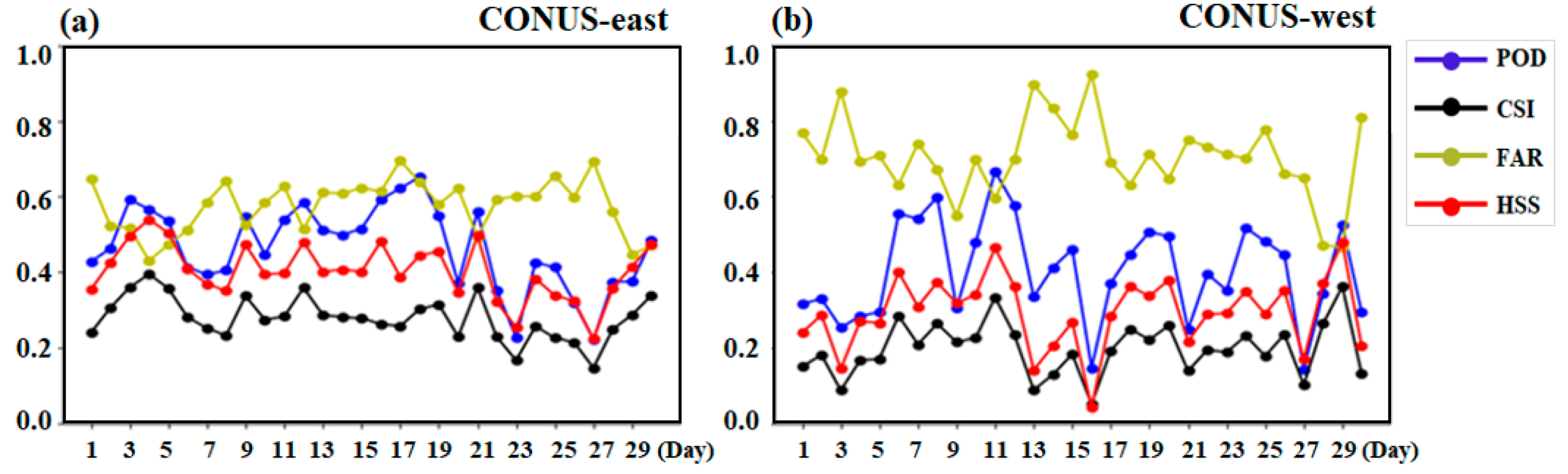
Figure 9 further shows the day-to-day variations of hourly detection skill metrics in September 2019 over CONUS-east and CONUS-west. This comparison also highlighted the distinct performances of the GOES-16 QPE across the two subregions. Compared to CONUS-east, the GOES-16 QPE exhibited a significantly higher
FAR over CONUS-west, indicating that the performance of the GOES-16 QPE was limited in that area. At the same time, this result may be due to the incomplete radar coverage of the MRMS system for CONUS-west.
From the quantitative evaluation results (not shown), for almost all days, the GORS-16 QPE hourly precipitation accumulations overestimated rainfall compared to the GC-MRMS product, although the quantitative evaluation results were small during days when heavy rain occurred. Notably, the best performance of the GOES-16 QPE occurred on 18 September 2019, when
POD was 0.75, and the
HSS and
FAR scores were 0.41 and 0.71, respectively (
Figure 9).
3.5. Heavy Rainfall Events
Figure 7 and
Figure 10 show the GOES-16 QPE and GC-MRMS estimated rainfall at specific times (0000 UTC on 8 May 2019 and 29 August 2018, respectively) over the CONUS. The cumulative one-day precipitation maps, as well as their differences, are also shown.
3.5.1. 29 August 2018 Event
Figure 10 compares CONUS-wide hourly (0000 UTC) and daily precipitation maps for the GOES-16 QPE and GC-MRMS on 29 August 2018. In this event, precipitation was mainly concentrated in CONUS-east. In terms of precipitation region and precipitation intensity, the GOES-16 QPE overestimated the rainy area and retrieved considerably more precipitation accumulations over the heavy rainfall center, compared to GC-MRMS. For CONUS-east, the hourly and maximum precipitation accumulations of GOES-16 were overestimated by 4 mm/h and 20 mm/h, respectively, from 0000 to 1000 UTC. However, GOES-16 generally overestimated precipitation accumulation by only 2 mm/h over CONUS-west. Interestingly, GOES-16 underestimated hourly precipitation accumulations after 1000 UTC over CONUS-east. This underestimation likely occurred because the observed brightness temperature (BT) was relatively high in GOES-16, and GOES-16 has trouble detecting precipitation under warm clouds, leading to an underestimation of warm precipitation. This result may have also been caused by the shallow convection below the cloud top [
16], which should be investigated in future studies.
In terms of evaluation results for CONUS-east from 0000 to 1000 UTC, POD was 0.73 (maximum), HSS was 0.61 (at 0300 UTC), CSI increased by 0.2, and CC was 0.60 (at 0000 UTC), indicating that GOES-16 was in good agreement with the GC-MRMS QPE for precipitation accumulation and patterns. In particular, at 1000 UTC, the NME of hourly precipitation accumulation was 0, and the average hourly precipitation accumulation of GC-MRMS products was 10 mm/h. After 1000 UTC, CC decreased to 0.33 at 1700 UTC, which implied that the precipitation evaluation of GOES-16 became poor.
3.5.2. 8 May 2019 Event
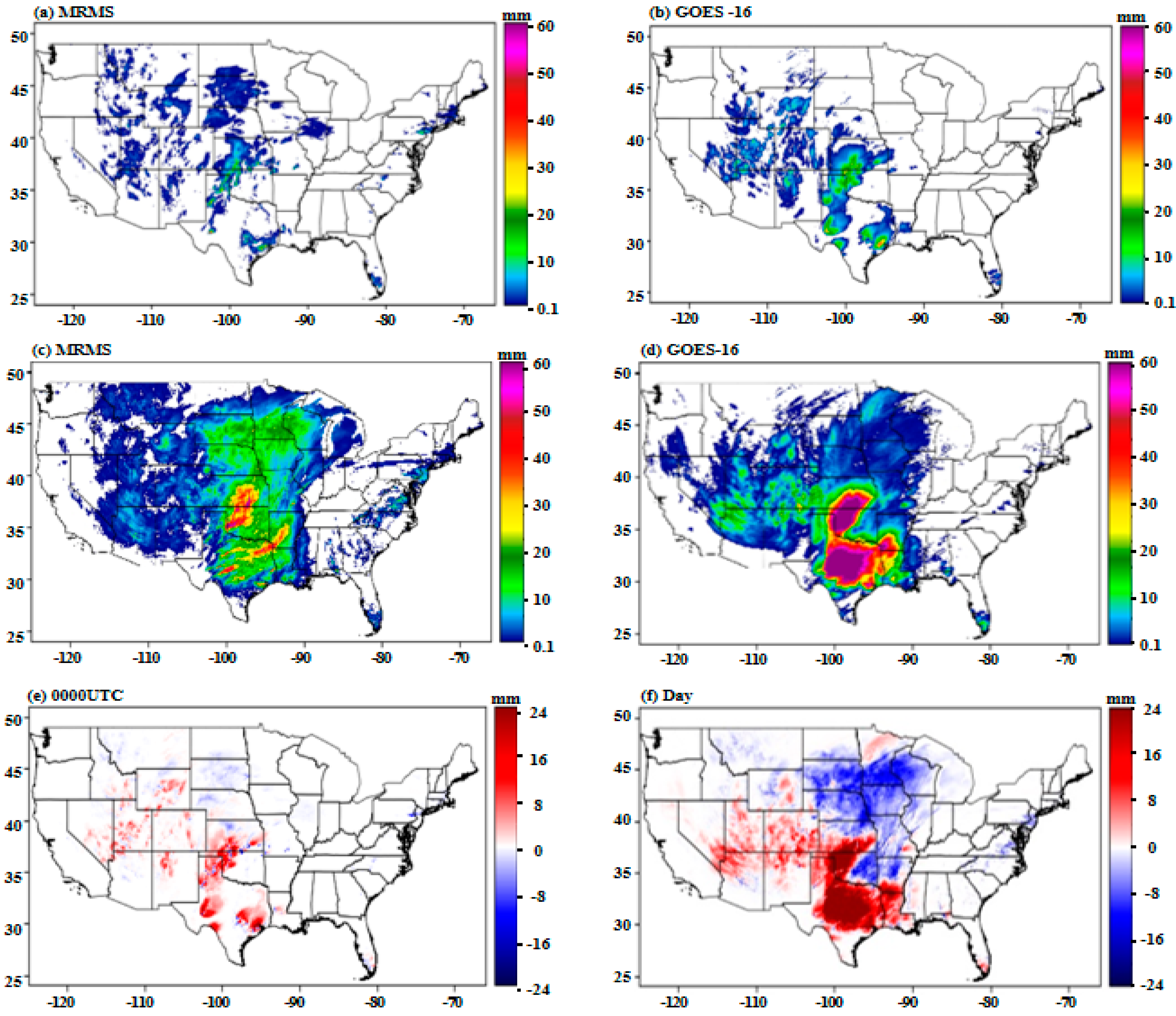
Figure 7a–d present hourly and daily precipitation accumulation from the GOES-16 and MRMS systems over CONUS on 8 May 2019.
Figure 7e,f show the corresponding differences between the two QPE products at 0000 UTC and for the entire day. During these precipitation events, CONUS-east and CONUS-west both experienced heavy rain, while the heaviest precipitation appeared primarily in CONUS-east. In terms of the precipitation region and precipitation intensity from 0000 to 0700 UTC in CONUS-east, the hourly precipitation accumulation of GOES-16 was mostly overestimated by 2 mm/h, with a maximum overestimation of 20 mm/h. For CONUS-west, GOES-16 generally overestimated hourly precipitation accumulation by 2 mm/h. In dry areas, GOES-16 observations produced a significant value of
FAR due to sub-cloud evaporation under the low BT cloud. Overall, GOES-16 overestimated precipitation intensity over regions in which BT was low because of the precipitating cloud, resulting in an overestimation of hourly precipitation accumulations.
In addition, the POD (maximum) was 0.55 (at 0500 UTC), with 0.53 (minimum at 0700 UTC) over CONUS-east during 0000 to 0700 UTC. CSI increased by 0.1, and CC was 0.61 (at 0700 UTC), indicating a reasonable correlation between the GOES-16 and GC-MRMS products. At 0700 UTC, NME was 0.04 (minimum); however, after 0700 UTC, the CSI value was 0.22 (at 1100 UTC), and GOES-16 underestimated precipitation, because shallow precipitation was not observed well. CC fell to 0.38 at 1300 UTC, illustrating significant differences between the GOES-16 and GC-MRMS products.
4. Discussion
The GOES-16 QPE was validated against the ground reference GC-MRMS data in this study. In general, the GOES-16 QPE reasonably captured both precipitation occurrence and intensity. Similar to other satellite QPE products, the uncertainty of the GOES-16 QPE increased as the analysis time scale decreased from seasonal to hourly. In addition, the present GOES-16 QPE algorithm (i.e., SCaMPR) was found to have different skills over CONUS-east and CONUS-west. The overall assessment results showed that GOES-16 tended to overestimate precipitation across different time scales, while it may also have underestimated hourly precipitation during the heavy rainfall events. It should be noted that the results presented here only focused on accumulated precipitation amounts from seasonal to hourly scales, and the performance of the GOES-16 QPE for estimating instantaneous (i.e., its native scale) precipitation rate must be explored in the future.
4.1. Orographic and Warm-Cloud Precipitation
Although significant efforts have been made to enhance the GOES-16 QPE algorithm, the detection of orographic precipitation remains challenging due to the difficulty of IR imagers to detect the high and cold cloud tops associated with orographic rainfall [
17]. The highly varied nature of clouds and other environmental factors (e.g., changes in the warm and humid airflows) over complex terrains limit the performance of the GOES-16 QPE over the mountainous western US. Though the different cloud types have been considered in the current GOES-16 QPE algorithm [
4], it can be further enhanced in the future for a better characterization of orographic precipitation.
In addition, our evaluation also suggested that rainfall associated with warm clouds is often overlooked (e.g.,
Figure 7). This phenomenon may occur when the GOES-16 ABI imager observes cloud tops with a high TB, while it cannot capture the airflow conditions under the cloud. This condition will naturally lead to an underestimation of the precipitation. Thus, cloud-top temperature alone is inadequate for correctly estimating various types of rainfall, and additional cloud-precipitation features should be considered to this end. Chen et al. made efforts to distinguish rain clouds from warm clouds without rain using characteristic cloud information [
18]. In addition, the relationship between precipitation and relative humidity may change due to the evaporation of water vapor from the sub-cloud top over dry regions such as the western US [
19]. Future works also need to further explore the relationship between the instantaneous precipitation rate and humidity adjustments, and to consider its impacts in precipitation evaluation.
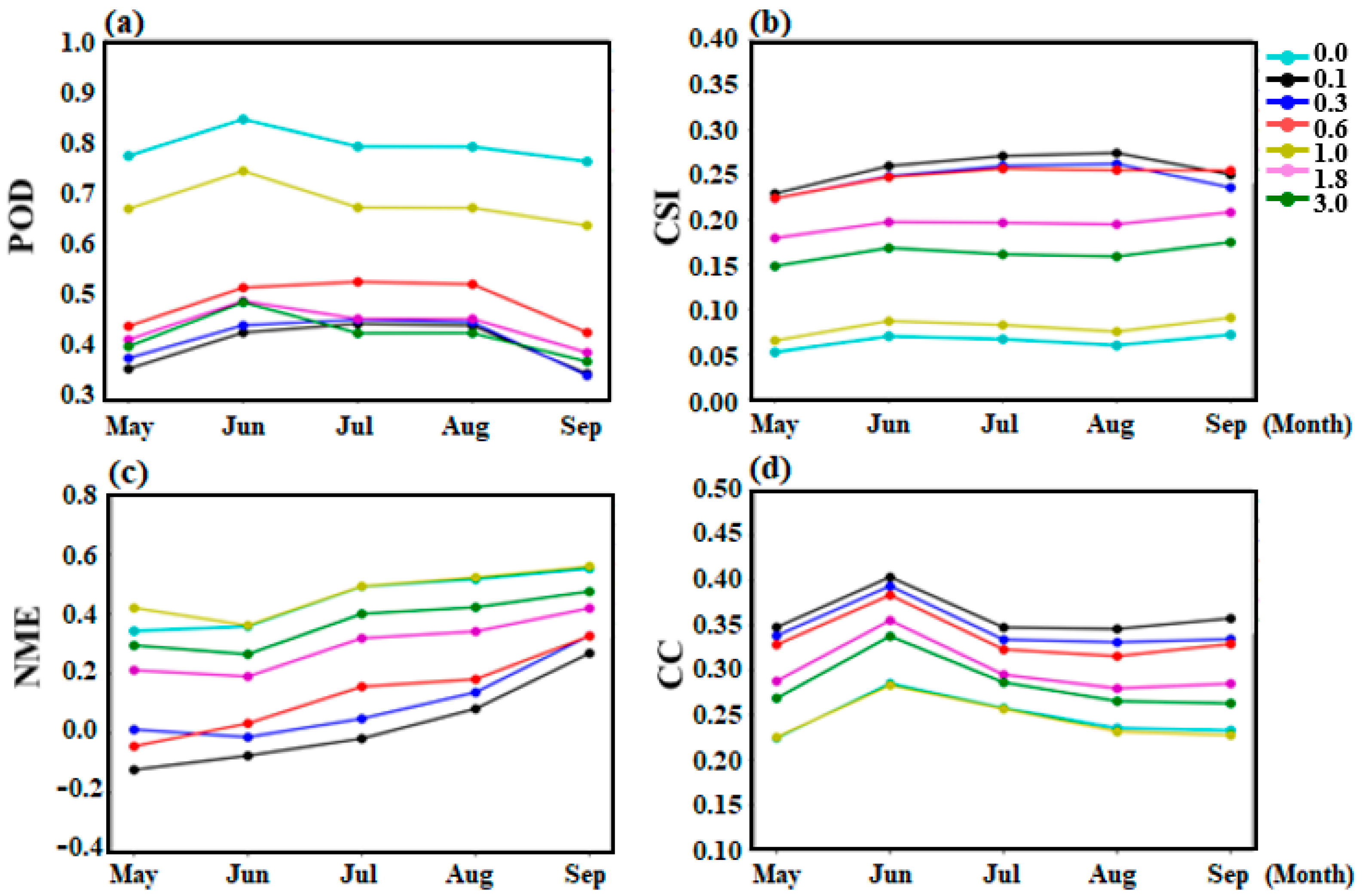
4.2. Rain/No-Rain Threshold for Evaluation
This study explored whether different rain/no-rain thresholds affected the evaluation results. The thresholds of hourly precipitation accumulation were set as 0, 0.1, 0.3, 0.6, 1.0, 1.8, and 3.0 mm/h, and the evaluation scores under different thresholds were calculated.
Figure 11 compares these evaluation scores, both detection skills and intensity estimation errors, for May to September 2018 over CONUS-east. Since the evaluation results for CONUS-west may have been affected by the terrains and many factors as mentioned above, this discussion of the rain/no-rain threshold selection thus only focuses on CONUS-east.
From May to September, the best scores for the four metrics were 0.85 (POD), 0.1 (CSI), 0.35 (NME), and 0.25 (CC) when the threshold was 0 mm/h. When the threshold was increased from 0 to 3.0 mm/h, the detection skills (in terms of POD) degraded, while other evaluation scores improved first (with the best scores when the threshold was 0.1~0.3 mm/h) and then degraded. These findings indicated that when the threshold was lower, the overall evaluation results tended to be better. In particular, when the threshold was set at 0.1~0.3 mm/h, most of the evaluation statistics had the best expected POD. The best performance based on POD was detected under the threshold of 0 mm/h, most likely because all of the precipitation events identified by GC-MRMS could be observed by the GOES-16 QPE without any lighter rainfall being ignored. Therefore, in this study, the spatiotemporal analysis was conducted using an hourly rain/no-rain threshold of 0.1 mm/h.
4.3. Uncertainty of the Reference
Though GC-MRMS has been widely used as the ground reference over CONUS, its limitation as a verification standard is well recognized, particularly in the mountainous western US. Compared with the results for CONUS-east, the performance of the GOES-16 QPE dropped significantly in terms of the complex mountainous regions over CONUS-west (e.g.,
Figure 9;
Table 4,
Table 5,
Table 6 and
Table 7). This most likely also was caused by the uncertainties related to GC-MRMS over the complex terrains, including the beam blockage, anomalous propagation, and ground clutter [
20,
21].
4.4. Other Uncertainties
It should be noted that this evaluation study was only based on two-year data records due to the limited availability of GOES-16 QPE data. Due to this short study period, many important issues were left to be addressed in the future. One of the major limitations was that the present study only examined warm-season precipitation, while different precipitation types and their impacts on GOES-16 performance were not explored. However, these factors can play an important role in determining a satellite QPE’s accuracy. In addition, the evaluation also was limited by the temporal resolution of GC-MRMS (1 h). In this paper, the GOES-16 QPE instantaneous precipitation rate (10 min) was converted into hourly precipitation accumulations, and then hourly accumulations were further aggregated into daily, monthly, and seasonal scales for evaluation. This integration inevitably introduced mathematical theory calculation errors. In addition, localized convective weather may only produce high-intensity rainfall during a very short periods, which could not be resolved by the 1 h time interval. Therefore, a more complete and robust approach for evaluation at finer time scales is needed in the future.
5. Concluding Remarks
Precipitation observation and estimation are critical to understanding the global and regional hydrological cycle. The new-generation geostationary GOES-16 satellite offers opportunities of high temporal (every 10 min) and spatial (2 km) resolution QPE over the globe, and therefore, the GOES-16 QPE holds great potential for providing critical input information for data-sparse regions, such as the ocean, complex terrains, and developing countries. In this study, the GOES-16 QPE was comprehensively evaluated using the NOAA’s GC-MRMS as the reference over the CONUS. This evaluation was conducted in the warm season (May to September) of 2018 and 2019, and a number of different evaluation metrics were applied to evaluate the performance of the GOES-16 QPE at hourly to seasonal scales. Primary conclusions are summarized as follows:
(1) In general, the GOES-16 QPE was consistent with GC-MRMS. Based on the evaluation results at different time scales, it was concluded that the ABI system on GOES-16 could detect most heavy precipitation events in space and time with reliable performance.
(2) The performance of the GOES-16 QPE varied significantly between CONUS-east and CONUS-west. Overall, the GOES-16 QPE showed better skills in the eastern United States than in the western United States. This regional difference could be partly attributed to the downgraded performance of the MRMS system over the western United States. In addition, the GOES-16 QPE could not accurately observe shallow precipitation events under clouds in arid areas, such as CONUS-west. Therefore, future development of the GOES-16 QPE retrieval algorithm should consider these critical aspects, as well as more observational information than just IR brightness temperature.
(3) Precipitation data during the warm seasons of 2018 and 2019 were used to evaluate the GOES-16 precipitation estimation. The GC-MRMS data were a fusion of multiple datasets, with ground-based radar as the primary observation mode, assisted by rain gauge information. Using MRMS products for verification, high-quality QPE from GOES-16 could be obtained for the southeast plains in the eastern United States. However, in the mountainous region of the western United States, GC-MRMS exposed a considerable disadvantage: lower coverage of observation equipment due to complex terrain produced errors in precipitation observations. Thus, errors in source data of the MRMS system were an essential reason for the differences observed between sub-domains. However, with the continuous popularization and improvement of dual-polarization radar, a more detailed QPE evaluation of the western region will likely be achieved soon.
Future development of the GOES-16 satellite precipitation algorithm should consider the above findings and limitations. Considering the promising results for satellite QPE by using a machine-learning approach, future GOES-16 QPE algorithm development can also take advantage of the power of machine learning to better characterize the spatiotemporal features of the precipitation system, and incorporate other environmental factors such as the terrains. This can further improve the accuracy of the GOES-16 QPE. In addition, other more accurate, high-resolution ground precipitation standards can be used to evaluate the GOES-16 QPE at finer scales, to fully characterize the error structure associated with the GOES-16 QPE.
Author Contributions
Conceptualization and supervision, H.C. and L.H.; formal analysis, L.S.; writing–original draft preparation, L.S. and Z.L.; writing–review and editing, H.C. and L.H. All authors have read and agreed to the published version of the manuscript.
Funding
L.S. and L.H. were supported by the National Natural Science Foundation of China under Grant No. 41875049, and the National Key R&D Program of China under Grant No. 2018YFC1507504. The work of H.C. and Z.L. was supported by Colorado State University and the NOAA Joint Polar Satellite System (JPSS) program through Grant No. NA19OAR4320073.
Institutional Review Board Statement
Not applicable.
Informed Consent Statement
Not applicable.
Data Availability Statement
Not applicable.
Acknowledgments
The authors would like to thank the anonymous reviewers for providing careful review and comments on this article. The discussion with Rob Cifelli from NOAA Physical Sciences Laboratory is also acknowledged.
Conflicts of Interest
The authors declare no conflict of interest.
References
- Vicente, G.A.; Scofield, R.A.; Menzel, W.P. The Operational GOES Infrared Rainfall Estimation Technique. Bull. Am. Meteorol. Soc. 1998, 79, 1883–1898. [Google Scholar] [CrossRef]
- Kummerow, C.; Hong, Y.; Olson, W.S.; Yang, S.; Adler, R.F.; Mccollum, J.; Ferraro, R.; Petty, G.; Shin, D.-B.; Wilheit, T.T. The Evolution of the Goddard Profiling Algorithm (GPROF) for Rainfall Estimation from Passive Microwave Sensors. J. Appl. Meteorol. 2001, 40, 1801–1820. [Google Scholar] [CrossRef]
- Joyce, R.J.; Janowiak, J.E.; Arkin, P.A.; Xie, P. CMORPH: A method that produces global precipitation estimates from passive microwave and infrared data at high spatial and temporal resolution. J. Hydrometeor. 2004, 5, 487–503. [Google Scholar] [CrossRef]
- Kuligowski, R.J. GOES-R Advanced Baseline Imager (ABI) Algorithm Theoretical Basis Document for Rainfall Rate (QPE); NO-AA/NESDIS/STAR Version 2.6; NO-AA STAR: Washington, DC, USA, 24 October 2013. [Google Scholar]
- Xie, P.; Joyce, R.; Wu, S.; Yoo, S.-H.; Yarosh, Y.; Sun, F.; Lin, R. Reprocessed, Bias-Corrected CMORPH Global High-Resolution Precipitation Estimates from 1998. J. Hydrometeorol. 2017, 18, 1617–1641. [Google Scholar] [CrossRef]
- Huffman, G.J.; Bolvin, D.T.; Nelkin, E.J.; Wolff, D.B.; Adler, R.F.; Gu, G.; Hong, Y.; Bowman, K.P.; Stocker, E.F. The TRMM Multisatellite Precipitation Analysis (TMPA): Quasi-Global, Multiyear, Combined-Sensor Precipitation Estimates at Fine Scales. J. Hydrometeorol. 2007, 8, 38–55. [Google Scholar] [CrossRef]
- Derin, Y.; Anagnostou, E.; Berne, A.; Borga, M.; Boudevillain, B.; Buytaert, W.; Chang, C.-H.; Chen, H.; Delrieu, G.; Hsu, Y.C.; et al. Evaluation of GPM-era Global Satellite Precipitation Products over Multiple Complex Terrain Regions. Remote Sens. 2019, 11, 2936. [Google Scholar] [CrossRef] [Green Version]
- Chen, H.; Chandrasekar, V.; Cifelli, R.; Xie, P. A Machine Learning System for Precipitation Estimation Using Satellite and Ground Radar Network Observations. IEEE Trans. Geosci. Remote Sens. 2019, 58, 982–994. [Google Scholar] [CrossRef]
- Ma, Y.; Sun, X.; Chen, H.; Hong, Y.; Zhang, Y. A two-stage blending approach for merging multiple satellite precipitation estimates and rain gauge observations: An experiment in the northeastern Tibetan Plateau. Hydrol. Earth Syst. Sci. 2021, 25, 359–374. [Google Scholar] [CrossRef]
- Kuligowski, R.J. A Self-Calibrating Real-Time GOES Rainfall Algorithm for Short-Term Rainfall Estimates. J. Hydrometeorol. 2002, 3, 112–130. [Google Scholar] [CrossRef]
- Zhang, J. Coauthors. National Mosaic and Multi Sensor QPE (NMQ) system: Description, results, and future plans. Bull. Am. Meteorol. Soc. 2011, 92, 1321–1338. [Google Scholar] [CrossRef] [Green Version]
- Kirstetter, P.-E.; Hong, Y.; Gourley, J.J.; Chen, S.; Flamig, Z.; Zhang, J.; Schwaller, M.; Petersen, W.; Amitai, E. Toward a Framework for Systematic Error Modeling of Spaceborne Precipitation Radar with NOAA/NSSL Ground Radar–Based National Mosaic QPE. J. Hydrometeorol. 2012, 13, 1285–1300. [Google Scholar] [CrossRef]
- Wen, Y.; Behrangi, A.; Chen, H.; Lambrigtsen, B. How well were the early 2017 California atmospheric river precipitation events captured by satellite products and ground-based radars? Quart. J. Roy. Meteorol. Soc. 2018, 144, 344–359. [Google Scholar] [CrossRef] [Green Version]
- Cocks, S.B.; Zhang, J.; Martinaitis, S.M.; Qi, Y.; Kaney, B.; Howard, K. MRMS QPE Performance East of the Rockies during the 2014 Warm Season. J. Hydrometeorol. 2017, 18, 761–775. [Google Scholar] [CrossRef]
- Stenz, R.; Dong, X.; Xi, B.; Kuligowski, R.J. Assessment of SCaMPR and NEXRAD Q2 Precipitation Estimates Using Oklahoma Mesonet Observations. J. Hydrometeorol. 2014, 15, 2484–2500. [Google Scholar] [CrossRef]
- Kuligowski, R.J.; Li, Y.; Hao, Y.; Zhang, Y. Improvements to the GOES-R Rainfall Rate Algorithm. J. Hydrometeorol. 2016, 17, 1693–1704. [Google Scholar] [CrossRef]
- Vicente, G.A.; Davenport, J.C.; Scofield, R.A. The role of orographic and parallax corrections on real time high resolution satellite rain rate distribution. Int. J. Remote Sens. 2002, 23, 221–230. [Google Scholar] [CrossRef]
- Chen, R.; Li, Z.; Kuligowski, R.J.; Ferraro, R.; Weng, F. A study of warm rain detection using A-Train satellite data. Geophys. Res. Lett. 2011, 38. [Google Scholar] [CrossRef] [Green Version]
- Stenz, R.; Dong, X.; Xi, B.; Feng, Z.; Kuligowski, R.J. Improving Satellite Quantitative Precipitation Estimation Using GOES-Retrieved Cloud Optical Depth. J. Hydrometeorol. 2016, 17, 557–570. [Google Scholar] [CrossRef]
- Chen, H.; Cifelli, R.; Chandrasekar, V.; Ma, Y. A Flexible Bayesian Approach to Bias Correction of Radar-Derived Precipitation Estimates over Complex Terrain: Model Design and Initial Verification. J. Hydrometeorol. 2019, 20, 2367–2382. [Google Scholar] [CrossRef]
- Chen, H.; Cifelli, R.; White, A. Improving Operational Radar Rainfall Estimates Using Profiler Observations Over Complex Terrain in Northern California. IEEE Trans. Geosci. Remote Sens. 2019, 58, 1821–1832. [Google Scholar] [CrossRef]
Figure 1.
The digital elevation model (DEM) map over the CONUS. The thick black line indicates the meridian 105°W, which divided the study domain into CONUS-east and CONUS-west.
Figure 1.
The digital elevation model (DEM) map over the CONUS. The thick black line indicates the meridian 105°W, which divided the study domain into CONUS-east and CONUS-west.
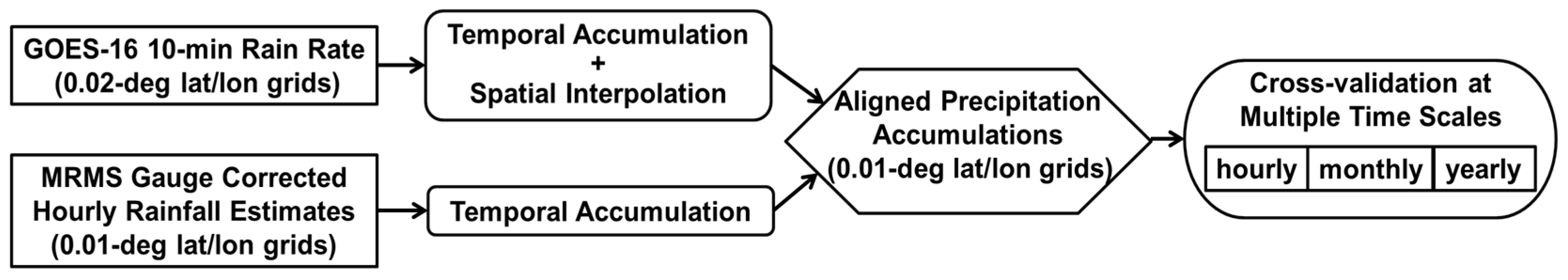
Figure 2.
Simplified flow chart of the space–time alignments of the GOES-16 QPE and GC-MRMS data.
Figure 2.
Simplified flow chart of the space–time alignments of the GOES-16 QPE and GC-MRMS data.
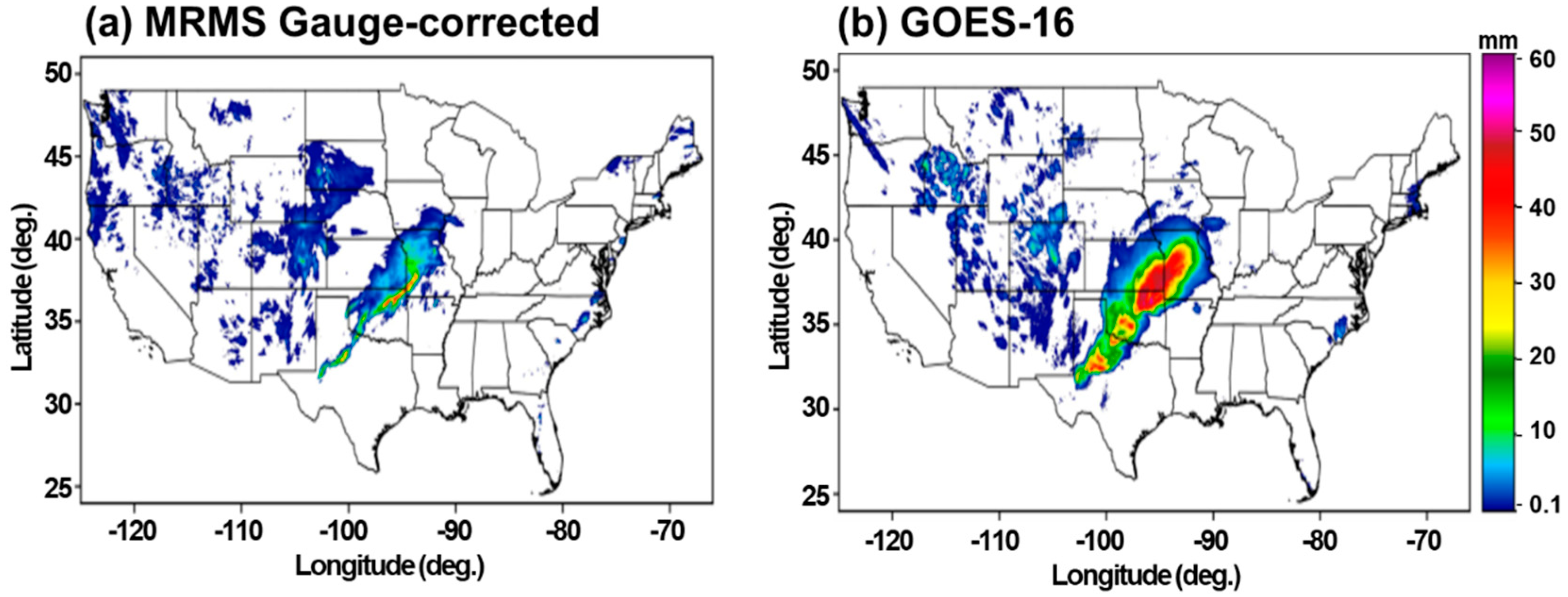
Figure 3.
The comparison of hourly precipitation estimates from: (a) GC-MRMS; and (b) interpolated GOES-16 QPE for 0200–0300 UTC on 21 May 2019.
Figure 3.
The comparison of hourly precipitation estimates from: (a) GC-MRMS; and (b) interpolated GOES-16 QPE for 0200–0300 UTC on 21 May 2019.
Figure 4.
Total rainfall accumulations during the warm season (May to September) in (a) 2018 and (b) 2019. From left to right, the columns are: GC-MRMS, GOES-16 QPE, PDF of seasonal precipitation accumulations, and the difference between GOES-16 QPE and GC-MRMS (the former minus the latter).
Figure 4.
Total rainfall accumulations during the warm season (May to September) in (a) 2018 and (b) 2019. From left to right, the columns are: GC-MRMS, GOES-16 QPE, PDF of seasonal precipitation accumulations, and the difference between GOES-16 QPE and GC-MRMS (the former minus the latter).
Figure 5.
The comparison of monthly rainfall accumulations from the GOES-16 QPE and GC-MRMS during the warm season (May to September) in 2018. From top to bottom, the rows represent different months. From left to right, the columns are: GC-MRMS, GOES-16 QPE, PDF of monthly total rainfall, and the difference between GOES-16 QPE and GC-MRMS (the former minus the latter).
Figure 6.
The comparison of monthly rainfall accumulations from the GOES-16 QPE and GC-MRMS during the warm season (May to September) in 2019. From top to bottom, the rows represent different months. From left to right, the columns are: GC-MRMS, GOES-16 QPE, PDF of monthly total rainfall, and the difference between GOES-16 QPE and GC-MRMS (the former minus the latter).
Figure 7.
Rainfall accumulations from GC-MRMS and GOES-16 QPE for the 8 May 2019 event. From left to right: GC-MRMS and GOES-16 QPE; (a,b) are hourly precipitation accumulations at 0000 UTC; (c,d) are daily rainfall accumulations; and (e,f) are the differences between the GOES-16 QPE and GC-MRMS for hourly and daily rainfall accumulations.
Figure 8.
Month-by-month changes of the hourly evaluation results for GOES-16 QPE over CONUS-east in 2018 (top panels) and 2019 (bottom panels): (a,c) detection skill metrics; and (b,d) evaluation metrics for estimating rainfall intensity.
Figure 8.
Month-by-month changes of the hourly evaluation results for GOES-16 QPE over CONUS-east in 2018 (top panels) and 2019 (bottom panels): (a,c) detection skill metrics; and (b,d) evaluation metrics for estimating rainfall intensity.
Figure 9.
Day-to-day changes in hourly detection skill statistics for the GOES-16 QPE in September 2019 over: (a) CONUS-east; (b) CONUS-west.
Figure 9.
Day-to-day changes in hourly detection skill statistics for the GOES-16 QPE in September 2019 over: (a) CONUS-east; (b) CONUS-west.
Figure 10.
Rainfall accumulations from GC-MRMS and GOES-16 QPE for the 29 August 2018 event. From left to right: GC-MRMS and GOES-16 QPE; (a,b) are hourly precipitation accumulations at 0000 UTC; (c,d) are daily rainfall accumulations; and (e,f) are the differences between the GOES-16 QPE and GC-MRMS for hourly and daily rainfall accumulations.
Figure 11.
Evaluation statistics of the GOES-16 QPE hourly rainfall under different rain/no-rain thresholds over CONUS-east from May to September 2018: (a) POD; (b) CSI; (c) NME; and (d) CC.
Figure 11.
Evaluation statistics of the GOES-16 QPE hourly rainfall under different rain/no-rain thresholds over CONUS-east from May to September 2018: (a) POD; (b) CSI; (c) NME; and (d) CC.
Table 1.
Evaluation statistics for the GOES-16 QPE estimated warm-season rainfall accumulations in 2018 and 2019.
Table 1.
Evaluation statistics for the GOES-16 QPE estimated warm-season rainfall accumulations in 2018 and 2019.
| | 2018 | 2019 |
|---|
| | CONUS-East * | CONUS-West * | CONUS * | CONUS-East * | CONUS-West * | CONUS * |
|---|
| ME (mm) | 340 | 255 | 309 | 433 | 258 | 368 |
| NME (–) | 0.37 | 0.63 | 0.42 | 0.43 | 0.57 | 0.46 |
| NMAE (–) | 0.46 | 0.64 | 0.50 | 0.51 | 0.59 | 0.53 |
| RMSE (mm) | 529 | 333 | 467 | 651 | 324 | 554 |
| CC (–) | 0.46 | 0.80 | 0.59 | 0.45 | 0.69 | 0.65 |
| POD (–) | 1.00 | 0.99 | 1.00 | 1.00 | 1.00 | 1.00 |
| CSI (–) | 1.00 | 0.99 | 1.00 | 1.00 | 1.00 | 1.00 |
| FAR (–) | 0.00 | 0.00 | 0.00 | 0.00 | 0.00 | 0.00 |
| HSS (–) | 1.00 | 0.00 | 0.00 | 1.00 | 0.00 | 0.00 |
Table 2.
Evaluation results of monthly rainfall accumulations (CONUS-east *).
Table 2.
Evaluation results of monthly rainfall accumulations (CONUS-east *).
| | 2018 | 2019 |
|---|
| | May * | June * | July * | August * | September * | May * | June * | July * | August * | September * |
|---|
| ME | 80.8 | 119.9 | 73.5 | 68.1 | -1.5 | 77.7 | 92.8 | 93.8 | 116.1 | 52.7 |
| NME | 0.42 | 0.50 | 0.40 | 0.38 | -0.01 | 0.36 | 0.42 | 0.46 | 0.51 | 0.41 |
| NMAE | 0.54 | 0.59 | 0.53 | 0.49 | 0.46 | 0.54 | 0.56 | 0.54 | 0.61 | 0.52 |
| RMSE | 141.7 | 188.5 | 139.3 | 116.1 | 79.0 | 174.5 | 164.4 | 144.8 | 217.8 | 103.2 |
| CC | 0.30 | 0.44 | 0.44 | 0.38 | 0.59 | 0.70 | 0.16 | 0.49 | 0.50 | 0.80 |
| POD | 1.00 | 1.00 | 1.00 | 1.00 | 1.00 | 1.00 | 1.00 | 1.00 | 1.00 | 1.00 |
| CSI | 1.00 | 1.00 | 1.00 | 1.00 | 1.00 | 1.00 | 1.00 | 1.00 | 1.00 | 0.99 |
| FAR | 0.00 | 0.00 | 0.00 | 0.00 | 0.00 | 0.00 | 0.00 | 0.00 | 0.00 | 0.01 |
| HSS | 0.00 | 0.01 | 0.00 | 1.00 | 0.00 | 0.00 | 1.00 | 0.00 | 0.01 | 0.10 |
Table 3.
Evaluation results of monthly rainfall accumulations (CONUS-west *).
Table 3.
Evaluation results of monthly rainfall accumulations (CONUS-west *).
| | 2018 | 2019 |
|---|
| | May * | June * | July * | August * | September * | May * | June * | July * | August * | September * |
|---|
| ME | 78.95 | 34.0 | 84.17 | 50.1 | 13.3 | 52.9 | 66.1 | 52.6 | 54.4 | 34.1 |
| NME | 0.68 | 0.5 | 0.7 | 0.61 | 0.41 | 0.51 | 0.68 | 0.6 | 0.83 | 0.43 |
| NMAE | 0.69 | 0.59 | 0.71 | 0.64 | 0.66 | 0.60 | 0.7 | 0.64 | 0.65 | 0.53 |
| RMSE | 108.0 | 63.5 | 156.60 | 86.44 | 33.07 | 80.16 | 87.92 | 91.63 | 89.86 | 60.45 |
| CC | 0.78 | 0.79 | 0.79 | 0.78 | 0.51 | 0.69 | 0.63 | 0.80 | 0.65 | 0.64 |
| POD | 0.95 | 0.88 | 0.94 | 0.93 | 0.93 | 1.00 | 0.95 | 0.95 | 0.97 | 0.98 |
| CSI | 0.95 | 0.88 | 0.94 | 0.92 | 0.91 | 0.99 | 0.95 | 0.95 | 0.96 | 0.98 |
| FAR | 0.00 | 0.01 | 0.00 | 0.01 | 0.01 | 0.00 | 0.00 | 0.00 | 0.01 | 0.01 |
| HSS | 0.02 | 0.40 | 0.09 | 0.44 | 0.50 | 0.00 | 0.01 | 0.09 | 0.63 | 0.25 |
Table 4.
Evaluation results of daily rainfall accumulations (CONUS-east *).
Table 4.
Evaluation results of daily rainfall accumulations (CONUS-east *).
| 2018 | 2019 |
|---|
| | May | June | July | August | September | Average | May | June | July | August | September | Average |
|---|
| ME | 6.45 | 10.1 | 6.30 | 5.50 | 0.56 | 5.78 | 6.55 | 6.76 | 6.93 | 9.12 | 5.81 | 5.63 |
| NME | 0.44 | 0.48 | 0.43 | 0.38 | 0.01 | 0.35 | 0.31 | 0.40 | 0.42 | 0.51 | 0.39 | 0.41 |
| NMAE | 0.8 | 0.8 | 0.83 | 0.81 | 0.92 | 0.83 | 0.83 | 0.84 | 0.85 | 0.84 | 0.79 | 0.83 |
| RMSE | 18.27 | 24.46 | 19.99 | 17.09 | 17.42 | 19.43 | 22.51 | 21.06 | 19.45 | 24.83 | 19.15 | 17.90 |
| CC | 0.46 | 0.51 | 0.42 | 0.48 | 0.49 | 0.47 | 0.58 | 0.47 | 0.45 | 0.43 | 0.59 | 0.47 |
| POD | 0.75 | 0.76 | 0.77 | 0.76 | 0.79 | 0.77 | 0.80 | 0.77 | 0.72 | 0.73 | 0.72 | 0.73 |
| CSI | 0.60 | 0.61 | 0.62 | 0.62 | 0.56 | 0.60 | 0.59 | 0.63 | 0.60 | 0.59 | 0.55 | 0.58 |
| FAR | 0.25 | 0.25 | 0.24 | 0.23 | 0.34 | 0.26 | 0.31 | 0.22 | 0.22 | 0.24 | 0.30 | 0.26 |
| HSS | 0.56 | 0.56 | 0.58 | 0.58 | 0.53 | 0.56 | 0.50 | 0.53 | 0.56 | 0.54 | 0.57 | 0.56 |
Table 5.
Evaluation results of daily rainfall accumulations (CONUS-west *).
Table 5.
Evaluation results of daily rainfall accumulations (CONUS-west *).
| 2018 | 2019 |
|---|
| | May | June | July | August | September | Average | May | June | July | August | September | Average |
|---|
| ME | 5.91 | 3.63 | 7.13 | 5.22 | 1.85 | 4.78 | 3.80 | 4.71 | 4.19 | 4.21 | 2.72 | 3.93 |
| NME | 0.66 | 0.48 | 0.66 | 0.66 | 0.15 | 0.53 | 0.56 | 0.65 | 0.61 | 0.58 | 0.35 | 0.55 |
| NMAE | 0.85 | 0.88 | 0.86 | 0.87 | 1.24 | 0.94 | 0.88 | 0.86 | 0.86 | 0.92 | 0.92 | 0.89 |
| RMSE | 11.25 | 9.06 | 16.39 | 11.59 | 6.99 | 11.09 | 8.83 | 9.73 | 10.73 | 9.99 | 8.87 | 9.63 |
| CC | 0.36 | 0.39 | 0.37 | 0.33 | 0.20 | 0.33 | 0.24 | 0.35 | 0.38 | 0.29 | 0.37 | 0.33 |
| POD | 0.63 | 0.62 | 0.67 | 0.63 | 0.57 | 0.62 | 0.67 | 0.63 | 0.68 | 0.59 | 0.66 | 0.64 |
| CSI | 0.53 | 0.49 | 0.55 | 0.52 | 0.38 | 0.49 | 0.51 | 0.53 | 0.53 | 0.48 | 0.53 | 0.52 |
| FAR | 0.26 | 0.29 | 0.27 | 0.29 | 0.45 | 0.31 | 0.33 | 0.23 | 0.27 | 0.30 | 0.27 | 0.28 |
| HSS | 0.49 | 0.52 | 0.54 | 0.53 | 0.42 | 0.50 | 0.39 | 0.50 | 0.51 | 0.47 | 0.50 | 0.47 |
Table 6.
Evaluation results of hourly rainfall accumulations (CONUS-east).
Table 6.
Evaluation results of hourly rainfall accumulations (CONUS-east).
| 2018 | 2019 |
|---|
| | May | June | July | August | September | Average | May | June | July | August | September | Average |
|---|
| ME | 39.3 | 9.69 | 2.1 | 12.9 | 1.13 | 13.02 | 94.34 | 1.11 | 1.7 | 1.47 | 0.83 | 5.31 |
| NME | 0.6 | 0.56 | 0.45 | 0.48 | 0.32 | 0.48 | 0.8 | 0.69 | 0.72 | 0.75 | 0.61 | 0.49 |
| NMAE | 0.94 | 0.92 | 0.99 | 0.95 | 0.99 | 0.96 | 0.94 | 0.95 | 0.96 | 0.96 | 1.05 | 0.96 |
| RMSE | 17.63 | 18.77 | 5.76 | 20.64 | 4.67 | 13.49 | 4.98 | 2.61 | 3.66 | 2.78 | 1.85 | 3.176 |
| CC | 0.26 | 0.32 | 0.29 | 0.29 | 0.3 | 0.29 | 0.14 | 0.14 | 0.14 | 0.14 | 0.07 | 0.32 |
| POD | 0.44 | 0.46 | 0.47 | 0.47 | 0.53 | 0.47 | 0.31 | 0.34 | 0.32 | 0.32 | 0.29 | 0.45 |
| CSI | 0.25 | 0.28 | 0.27 | 0.28 | 0.24 | 0.26 | 0.19 | 0.2 | 0.19 | 0.2 | 0.13 | 0.27 |
| FAR | 0.61 | 0.55 | 0.58 | 0.57 | 0.68 | 0.6 | 0.65 | 0.67 | 0.67 | 0.64 | 0.79 | 0.57 |
| HSS | 0.35 | 0.39 | 0.38 | 0.39 | 0.34 | 0.37 | 0.27 | 0.28 | 0.27 | 0.29 | 0.2 | 0.38 |
Table 7.
Evaluation results of hourly rainfall accumulations (CONUS-west).
Table 7.
Evaluation results of hourly rainfall accumulations (CONUS-west).
| 2018 | 2019 |
|---|
| | May | June | July | August | September | Average | May | June | July | August | September | Average |
|---|
| ME | 94.34 | 1.11 | 1.7 | 1.47 | 0.83 | 19.89 | 1.19 | 1.27 | 1.2 | 2.46 | 6.16 | 2.46 |
| NME | 0.8 | 0.69 | 0.72 | 0.75 | 0.61 | 0.71 | 0.78 | 0.78 | 0.69 | 0.66 | 0.59 | 0.7 |
| NMAE | 0.94 | 0.95 | 0.96 | 0.96 | 1.05 | 0.97 | 0.94 | 0.96 | 0.97 | 1.02 | 0.99 | 0.98 |
| RMSE | 27.89 | 2.61 | 3.66 | 2.78 | 1.85 | 7.76 | 2.25 | 2.3 | 2.57 | 9.99 | 14.63 | 6.35 |
| CC | 0.14 | 0.14 | 0.14 | 0.14 | 0.07 | 0.13 | 0.1 | 0.12 | 0.16 | 0.13 | 0.15 | 0.13 |
| POD | 0.31 | 0.34 | 0.32 | 0.32 | 0.29 | 0.32 | 0.32 | 0.28 | 0.33 | 0.29 | 0.37 | 0.32 |
| CSI | 0.19 | 0.2 | 0.19 | 0.2 | 0.13 | 0.18 | 0.17 | 0.18 | 0.19 | 0.18 | 0.22 | 0.19 |
| FAR | 0.65 | 0.67 | 0.67 | 0.64 | 0.79 | 0.68 | 0.72 | 0.65 | 0.66 | 0.66 | 0.63 | 0.66 |
| HSS | 0.27 | 0.28 | 0.27 | 0.29 | 0.2 | 0.26 | 0.22 | 0.25 | 0.28 | 0.26 | 0.3 | 0.26 |
| Publisher’s Note: MDPI stays neutral with regard to jurisdictional claims in published maps and institutional affiliations. |
© 2021 by the authors. Licensee MDPI, Basel, Switzerland. This article is an open access article distributed under the terms and conditions of the Creative Commons Attribution (CC BY) license (https://creativecommons.org/licenses/by/4.0/).


