
Two-Stream Deep Fusion Network Based on VAE and CNN for Synthetic Aperture Radar Target Recognition


Abstract
:
1. Introduction
- Considering that both the SAR image and the corresponding HRRP data, in which the information contained are not exactly the same, can be simultaneously obtained in the procedure of SAR imaging, we apply two different sub-networks, VAE and LightNet, in the proposed deep fusion network to mine the different characteristics from the average profiles of the HRRP data and the SAR image, respectively. Through joint utilization of these two types of characteristics, the target representation is more comprehensive and sufficient, which is beneficial for the target recognition task. Moreover, the proposed network is a unified framework which can be end-to-end joint optimized.
- For the integration process on the latent feature of VAE and the structure feature of LightNet, a novel fusion module is developed in the proposed fusion network. The proposed fusion module takes advantage of the latent feature and the structure feature to automatically learn an attention weight. Then, the learned attention weight is used to adaptively integrate the latent feature and the structure feature. Compared with original concatenation operator, the proposed fusion module can achieve better recognition performance.
2. Related Work
2.1. Radar Target Recognition
2.2. Information Fusion
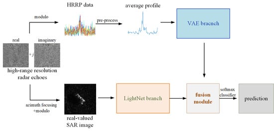
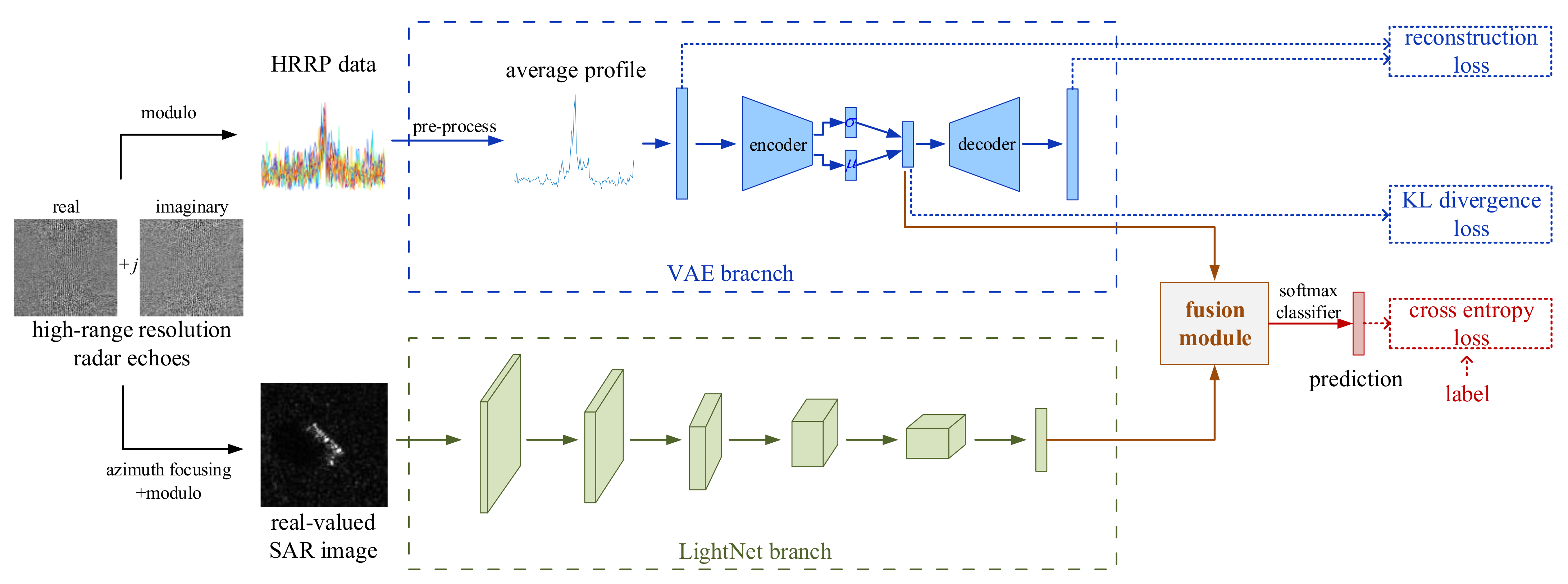
3. Two-Stream Deep Fusion Network Based on VAE and CNN
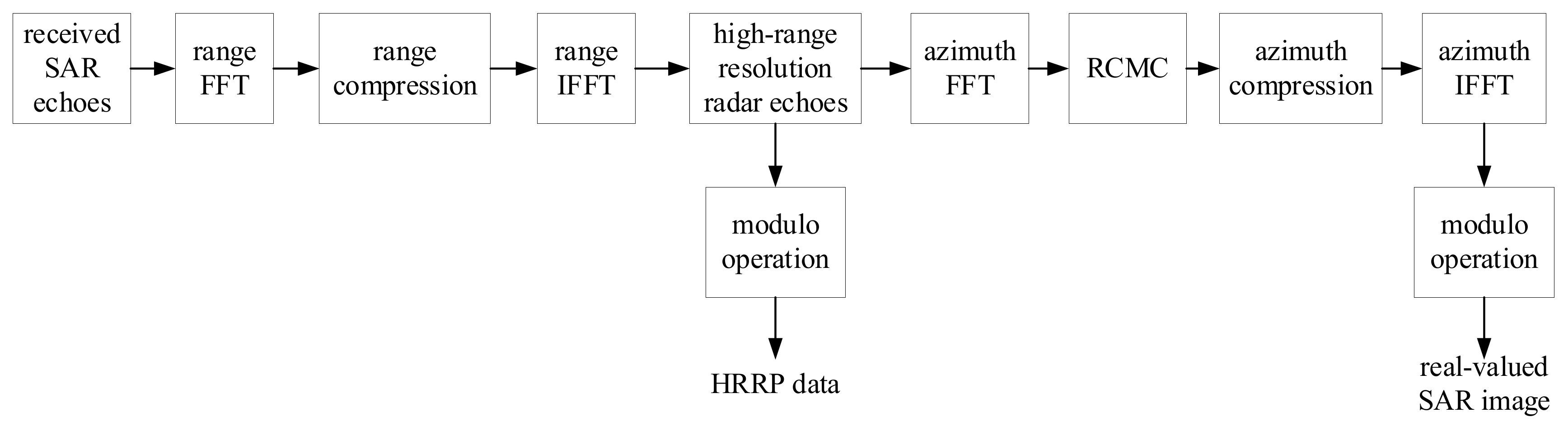
- Data acquisition: as can be seen from Figure 1, the complex-valued high-range resolution radar echoes can be obtained after range compression of the receiving SAR echoes. Then, the HRRP data are obtained through the modulo operation. At the same time, based on the complex-valued high-range resolution radar echoes, the complex-valued SAR image is obtained through azimuth focusing processing. Then, the commonly used real-valued SAR image for target recognition can be obtained by modulating the complex-valued SAR image.
- VAE branch: based on the HRRP data, the average profile of the HRRP is obtained by preprocessing. Then, the average profile is fed into the VAE branch to acquire the latent probabilistic distribution as a representation of the target information.
- LightNet branch: the other branch takes the SAR image as input and draws support from a lightweight convolutional architecture, LightNet, to extract the 2D visual structure information as another essential representation of the target information.
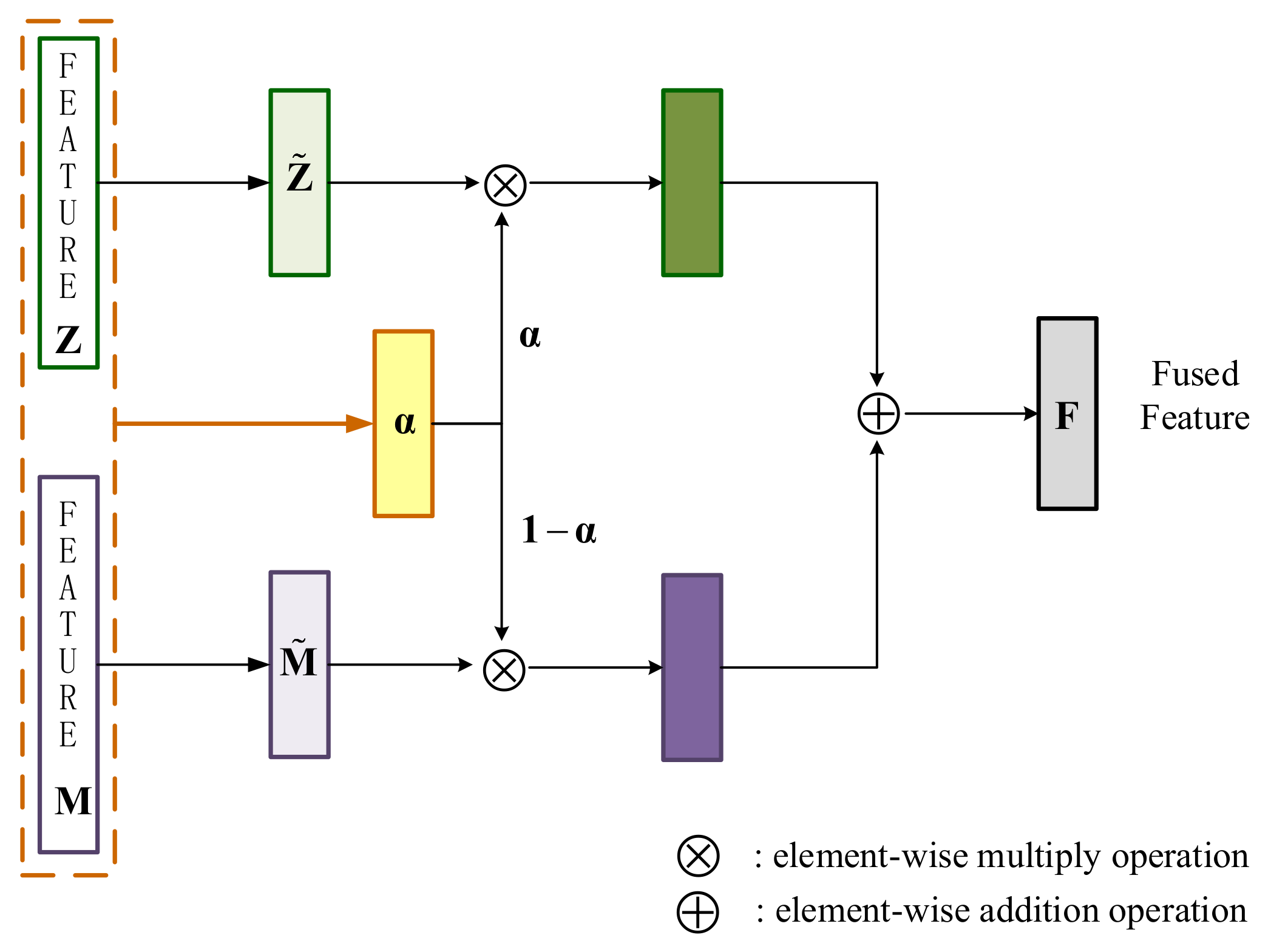
- Fusion module: the fusion module is employed to integrate the distribution representation and the visual structure representation to reflect more comprehensive and sufficient information for target recognition. The fusion module merges the VAE branch and the LightNet branch into a unified framework which can be trained in an end-to-end manner.
- Softmax classifier: finally, the integrated feature is fed into a usual softmax classifier to predict the category of target.
3.1. Acquisition of the HRRP Data and the Real-Valued SAR Image from High-Range Resolution Echoes
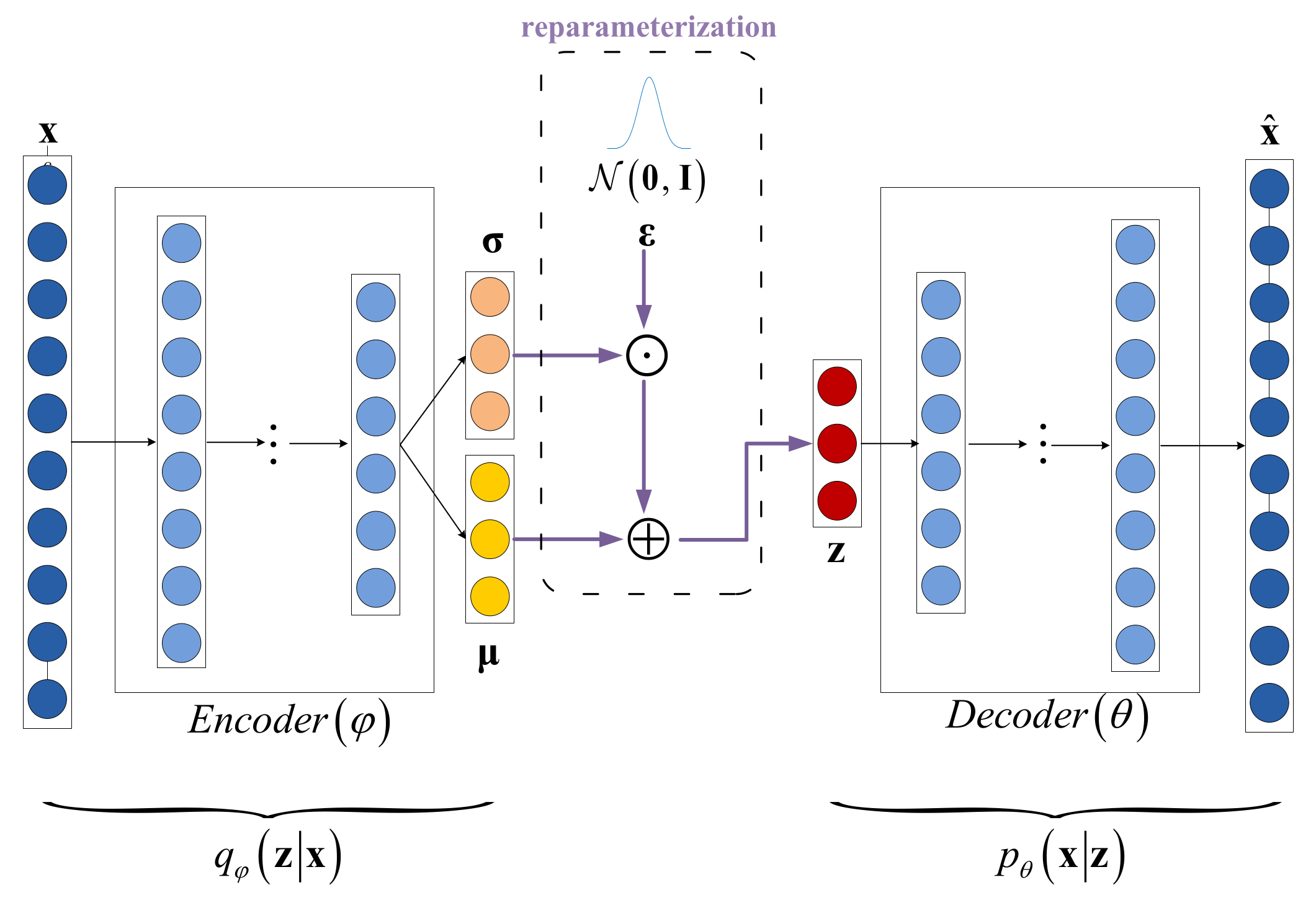
3.2. The VAE Branch
3.3. The LightNet Branch
3.4. Fusion Module
3.5. Loss Function
3.6. Training Procedure
| Algorithm 1. Training Procedure of the Proposed Network |
| 1. Set the architecture of the proposed network, including the number of fully connected layers, the units in each fully connected layer, the size of convolutional kernels, the strides and the number of channels, and so on. |
| 2. Initialize the network parameters , , , and . |
| 3. while not converged do |
| 4. Randomly sample a mini-batch and its corresponding label from the whole dataset. |
| 5. Based on each data in the mini-batch, generate the average profile and the SAR image . |
| 6. Sample random noise from standard Gaussian distribution for re-parameterization. |
| 7. With as input, generate the latent distribution representation using Equations (2) and (3), and then generate the reconstruction based on Equation (4). |
| 8. With as input, generate the structure information using Equation (11). |
| 9. Based on Equation (15), generate integrated feature . |
| 10. Based on integrated feature , obtain prediction with Equation (16). |
| 11. Compute the total loss . |
| 12. Update network parameters , , , and via SGD on the total loss . |
| 13. end while |
4. Results
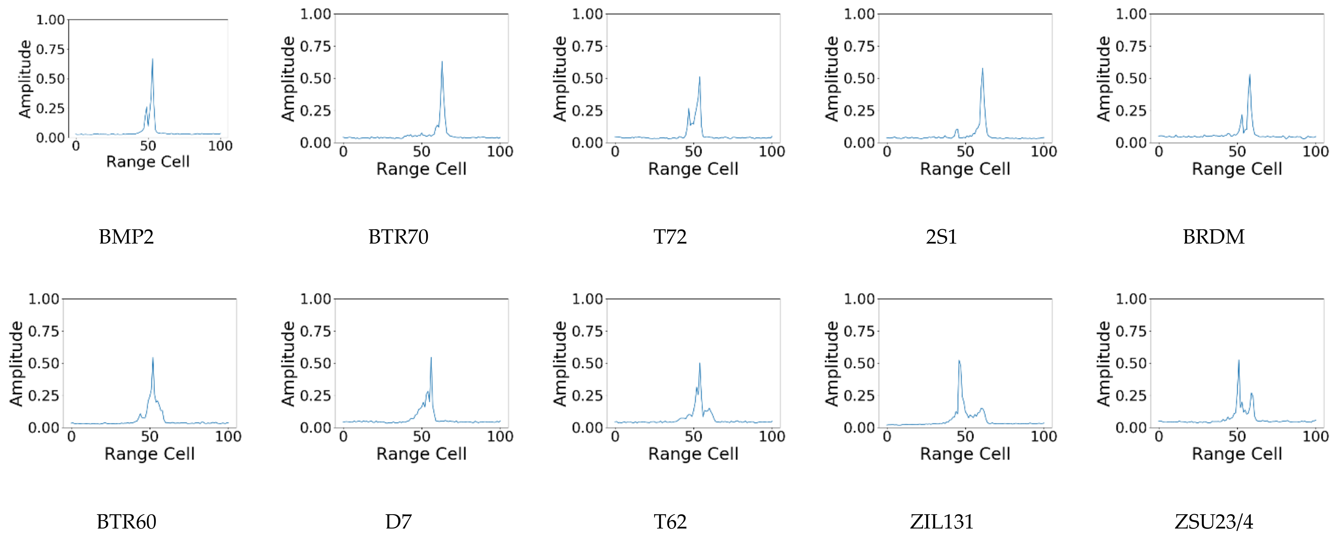
4.1. Experimental Data Description
4.2. Evaluation Criteria
4.3. Three-Target MSTAR Data Experiments
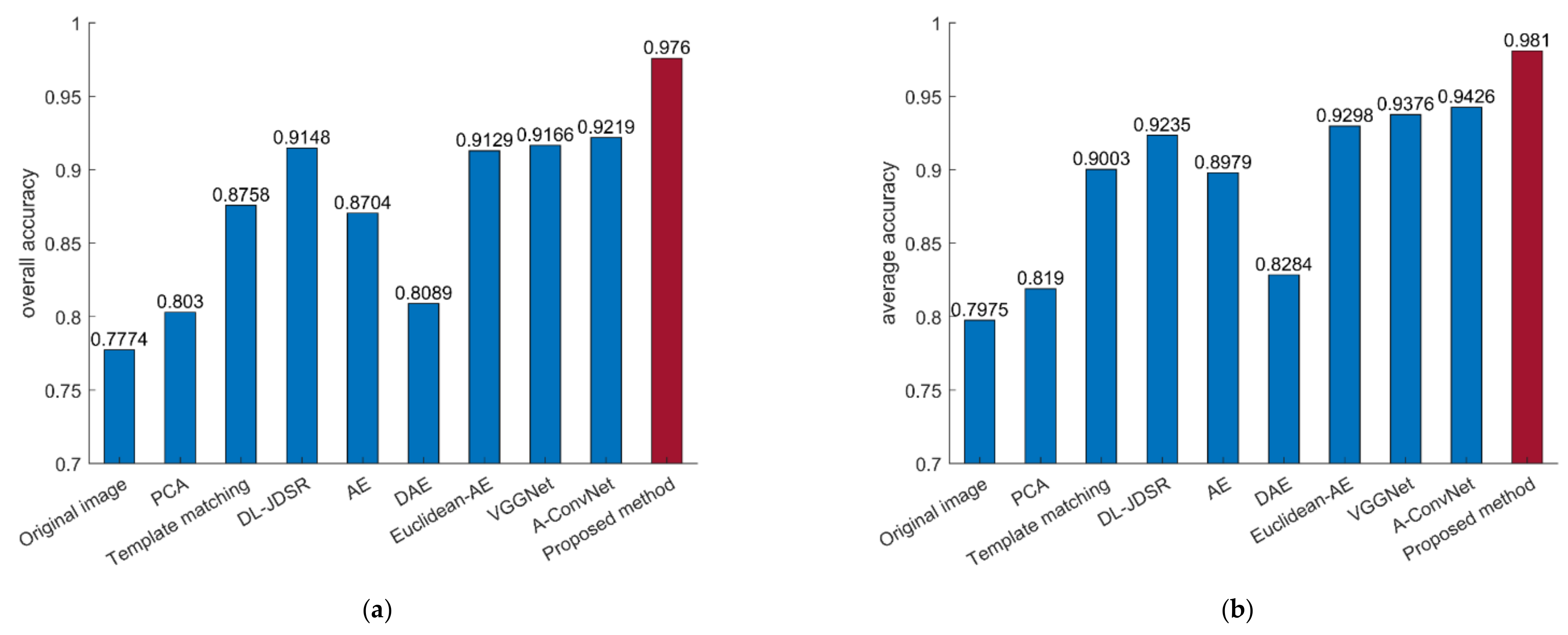
4.4. Ten-Target MSTAR Data Experiments
4.5. Model Analysis
4.5.1. Ablation Study
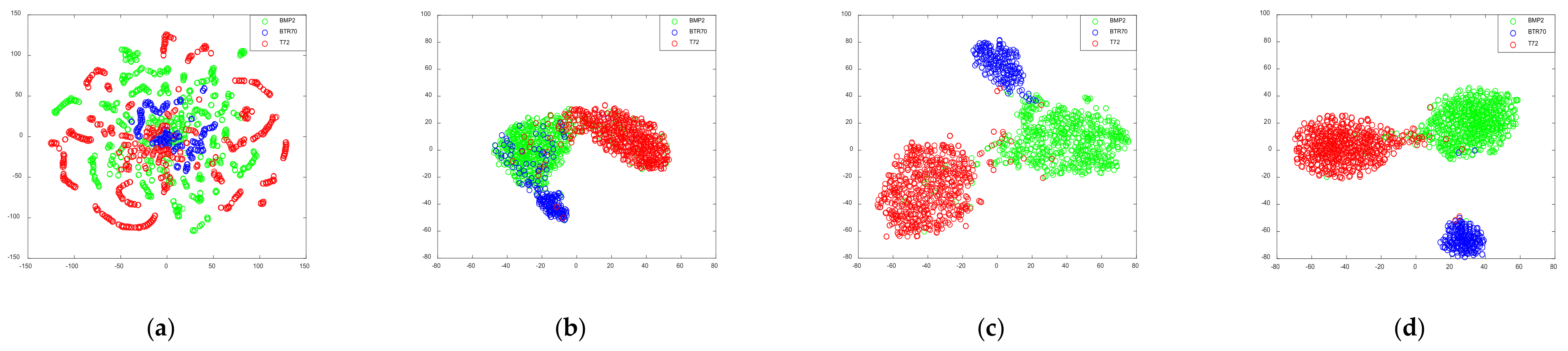
4.5.2. Feature Analysis
4.5.3. FLOPs Analysis
4.6. Experiments on Civilian Vehicle Dataset
5. Conclusions
Author Contributions
Funding
Data Availability Statement
Conflicts of Interest
References
- Chen, S.; Wang, H. SAR target recognition based on deep learning. In Proceedings of the International Conference on Data Science and Advanced Analytics (DSAA), Paris, France, 19–21 October 2015. [Google Scholar]
- Cui, Z.; Cao, Z.; Yang, J.; Ren, H. Hierarchical Recognition System for Target Recognition from Sparse Representations. Math. Probl. Eng. 2015, 2015 Pt 17, 6. [Google Scholar] [CrossRef]
- Deng, S.; Du, L.; Li, C.; Ding, J.; Liu, H. SAR automatic target recognition based on euclidean distance restricted autoencoder. IEEE J. Sel. Top. Appl. Earth Obs. Remote Sens. 2017, 10, 3323–3333. [Google Scholar] [CrossRef]
- Housseini, A.E.; Toumi, A.; Khenchaf, A. Deep Learning for Target recognition from SAR images. In Proceedings of the 2017 Seminar on Detection Systems Architectures and Technologies (DAT), Algiers, Algeria, 20–22 February 2017. [Google Scholar]
- Yan, H.; Zhang, Z.; Gang, X.; Yu, W. Radar HRRP recognition based on sparse denoising autoencoder and multi-layer perceptron deep model. In Proceedings of the 2016 Fourth International Conference on Ubiquitous Positioning, Indoor Navigation and Location Based Services (UPINLBS), Shanghai, China, 2–4 November 2016. [Google Scholar]
- Kingma, D.P.; Welling, M. Auto-Encoding Variational Bayes. arXiv 2013, arXiv:1312.6114. [Google Scholar]
- Du, C.; Chen, B.; Xu, B.; Guo, D.; Liu, H. Factorized Discriminative Conditional Variational Auto-encoder for Radar HRRP Target Recognition. Signal Process. 2019, 158, 176–189. [Google Scholar] [CrossRef]
- Du, L.; Liu, H.; Bao, Z.; Zhang, J. Radar automatic target recognition using complex high-resolution range profiles. IET Radar Sonar Navig. 2007, 1, 18–26. [Google Scholar] [CrossRef]
- Du, L. Noise Robust Radar HRRP Target Recognition Based on Multitask Factor Analysis With Small Training Data Size. IEEE Trans. Signal Process. 2012, 60, 3546–3559. [Google Scholar]
- Xing, M. Properties of high-resolution range profiles. Opt. Eng. 2002, 41, 493–504. [Google Scholar] [CrossRef]
- Zhang, X.Z.; Huang, P.K. Multi-aspect SAR target recognition based on features of sequential complex HRRP using CICA. Syst. Eng. Electron. 2012, 34, 263–269. [Google Scholar]
- Masahiko, N.; Liao, X.J.; Carin, L. Target identification from multi-aspect high range-resolution radar signatures using a hidden Markov model. IEICE Trans. Electron. 2004, 87, 1706–1714. [Google Scholar]
- Tan, X.; Li, J. Rang-Doppler imaging via forward- backward sparse Bayesian learning. IEEE Trans. Signal Process. 2010, 58, 2421–2425. [Google Scholar] [CrossRef]
- Zhao, F.; Liu, Y.; Huo, K.; Zhang, S.; Zhang, Z. Radar HRRP Target Recognition Based on Stacked Autoencoder and Extreme Learning Machine. Sensors 2018, 18, 173. [Google Scholar] [CrossRef] [PubMed] [Green Version]
- Feng, B.; Chen, B.; Liu, H. Radar HRRP target recognition with deep networks. Pattern Recognit. 2017, 61, 379–393. [Google Scholar] [CrossRef]
- Pan, M.; Liu, A.L.; Yu, Y.Z.; Wang, P.; Li, J.; Liu, Y.; Lv, S.S.; Zhu, H. Radar HRRP target recognition model based on a stacked CNN-Bi-RNN with attention mechanism. IEEE Trans. Geosci. Remote Sens. 2021, 61, 1–14, online published. [Google Scholar] [CrossRef]
- Chen, W.C.; Chen, B.; Peng, X.J.; Liu, J.; Yang, Y.; Zhang, H.; Liu, H. Tensor RNN with Bayesian nonparametric mixture for radar HRRP modeling and target recognition. IEEE Trans. Signal Process. 2021, 69, 1995–2009. [Google Scholar] [CrossRef]
- Peng, X.; Gao, X.Z.; Zhang, Y.F. An adaptive feature learning model for sequential radar high resolution range profile recognition. Sensors 2017, 17, 1675. [Google Scholar] [CrossRef] [PubMed] [Green Version]
- Jacobs, S.P. Automatic Target Recognition Using High-Resolution Radar Range-Profiles; ProQuest Dissertations Publishing: Morrisville, NC, USA, 1997. [Google Scholar]
- Webb, A.R. Gamma mixture models for target recognition. Pattern Recognit. 2000, 33, 2045–2054. [Google Scholar] [CrossRef]
- Copsey, K.; Webb, A. Bayesian gamma mixture model approach to radar target recognition. IEEE Trans. Aerosp. Electron. Syst. 2003, 39, 1201–1217. [Google Scholar] [CrossRef]
- Du, L.; Liu, H.; Zheng, B.; Zhang, J. A two-distribution compounded statistical model for Radar HRRP target recognition. IEEE Trans. Signal Process. 2006, 54, 2226–2238. [Google Scholar]
- Du, L.; Liu, H.; Bao, Z. Radar HRRP Statistical Recognition: Parametric Model and Model Selection. IEEE Trans. Signal Process. 2008, 56, 1931–1944. [Google Scholar] [CrossRef]
- Du, L.; Wang, P.; Zhang, L.; He, H.; Liu, H. Robust statistical recognition and reconstruction scheme based on hierarchical Bayesian learning of HRR radar target signal. Expert Syst. Appl. 2015, 42, 5860–5873. [Google Scholar] [CrossRef]
- Park, S.C.; Park, M.K.; Kang, M.G. Super-Resolution Image Reconstruction: A Technical Overview. IEEE Signal Process. Mag. 2003, 20, 21–36. [Google Scholar] [CrossRef] [Green Version]
- Wang, P.; Shi, L.; Lan, D.; Liu, H.; Xu, L.; Bao, Z. Radar HRRP Statistical Recognition With Local Factor Analysis by Automatic Bayesian Ying-Yang Harmony Learning. Front. Electr. Electron. Eng. China 2011, 6, 300–317. [Google Scholar] [CrossRef]
- Chen, J.; Du, L.; He, H.; Guo, Y. Convolutional factor analysis model with application to radar automatic target recognition. Pattern Recognit. 2019, 87, 140–156. [Google Scholar] [CrossRef]
- Pan, M.; Du, L.; Wang, P.; Liu, H.; Bao, Z. Noise-Robust Modification Method for Gaussian-Based Models With Application to Radar HRRP Recognition. IEEE Geosci. Remote Sens. Lett. 2013, 10, 55–62. [Google Scholar] [CrossRef]
- Chen, H.; Guo, Z.Y.; Duan, H.B.; Ban, D. A genetic programming-driven data fitting method. IEEE Access 2020, 8, 111448–111458. [Google Scholar] [CrossRef]
- Rezende, D.J.; Mohamed, S.; Wierstra, D. Stochastic Backpropagation and Approximate Inference in Deep Generative Models. In Proceedings of the International Conference on Machine Learning, Beijing, China, 21–26 June 2014. [Google Scholar]
- Doersch, C. Tutorial on Variational Autoencoders. arXiv 2016, arXiv:1606.05908. [Google Scholar]
- Ying, Z.; Bo, C.; Hao, Z.; Wang, Z. Robust Variational Auto-Encoder for Radar HRRP Target Recognition. In Proceedings of the International Conference on Intelligent Science & Big Data Engineering, Dalian, China, 22–23 September 2017. [Google Scholar]
- Chen, J.; Du, L.; Liao, L. Class Factorized Variational Auto-encoder for Radar HRRP Target Recognition. In Proceedings of the 2020 IEEE Radar Conference (RadarConf20), Florence, Italy, 21–25 September 2020. [Google Scholar]
- Simonyan, K.; Zisserman, A. Very deep convolutional networks for large-scale image recognition. arXiv 2014, arXiv:1409.1556. [Google Scholar]
- Min, R.; Lan, H.; Cao, Z.; Cui, Z. A Gradually Distilled CNN for SAR Target Recognition. IEEE Access 2019, 7, 42190–42200. [Google Scholar] [CrossRef]
- Huang, X.; Yang, Q.; Qiao, H. Lightweight two-stream convolutional neural network for SAR target recognition. IEEE Geosci. Remote Sens. Lett. 2020, 18, 667–671. [Google Scholar] [CrossRef]
- Cho, J.; Chan, G. Multiple feature aggregation using convolutional neural networks for SAR image-based automatic target recognition. IEEE Geosci. Remote Sens. Lett. 2018, 15, 1882–1886. [Google Scholar] [CrossRef]
- Ruser, H.; Leon, F.P. Information fusion—An overview. Tech. Mess. 2006, 74, 93–102. [Google Scholar] [CrossRef]
- Jiang, L.; Yan, L.; Xia, Y.; Guo, Q.; Fu, M.; Lu, K. Asynchronous multirate multisensor data fusion over unreliable measurements with correlated noise. IEEE Trans. Aerosp. Electron. Syst. 2017, 53, 2427–2437. [Google Scholar] [CrossRef]
- Rasti, B.; Ghamisi, P.; Plaza, J.; Plaza, A. Fusion of hyperspectral and LiDAR data using sparse and low-rank component analysis. IEEE Trans. Geosci. Remote Sens. 2017, 55, 6354–6365. [Google Scholar] [CrossRef] [Green Version]
- Bassford, M.; Painter, B. Intelligent bio-environments: Exploring fuzzy logic approaches to the honeybee crisis. In Proceedings of the 2016 12th International Conference on Intelligent Environments (IE), London, UK, 14–16 September 2016; IEEE: Piscataway, NJ, USA, 2016; pp. 202–205. [Google Scholar]
- Mehra, A.; Jain, N.; Srivastava, H.S. A novel approach to use semantic segmentation based deep learning networks to classify multi-temporal SAR data. Geocarto Int. 2020, 1–16. [Google Scholar] [CrossRef]
- Pei, J.; Huang, Y.; Huo, W.; Zhang, Y.; Yang, J.; Yeo, T.S. SAR automatic target recognition based on multiview deep learning framework. IEEE Trans. Geosci. Remote Sens. 2017, 56, 2196–2210. [Google Scholar] [CrossRef]
- Choi, I.O.; Jung, J.H.; Kim, S.H.; Kim, K.T.; Park, S.H. Classification of targets improved by fusion of range profile and the inverse synthetic aperture radar image. Prog. Electromagn. Res. 2014, 144, 23–31. [Google Scholar] [CrossRef] [Green Version]
- Wang, L.X.; Weng, L.G.; Xia, M.; Liu, J.; Lin, H. Multi-resolution supervision network with an adaptive weighted loss for desert segmentation. Remote Sens. 2021, 13, 1–18. [Google Scholar]
- Shang, R.H.; Zhang, J.Y.; Jiao, L.C.; Li, Y.; Marturi, N.; Stolkin, R. Multi-scale Adaptive feature fusion network for segmentation in remote sensing images. Remote Sens. 2020, 12, 872. [Google Scholar] [CrossRef] [Green Version]
- Chen, J.; He, F.; Zhang, Y.; Sun, G.; Deng, M. SPMF-net: Weakly supervised building segmentation by combining superpixel pooling and multi-scale feature fusion. Remote Sens. 2020, 12, 1049. [Google Scholar] [CrossRef] [Green Version]
- Liao, X.; Runkle, P.; Carin, L. Identification of ground targets from sequential high-range-resolution radar signatures. IEEE Trans. Aerosp. Electron. Syst. 2002, 38, 1230–1242. [Google Scholar] [CrossRef]
- Zhang, X.; Liu, Z.; Liu, S.; Li, G. Time-Frequency Feature Extraction of HRRP Using AGR and NMF for SAR ATR. J. Electr. Comput. Eng. 2015, 2015, 340–349. [Google Scholar] [CrossRef]
- Chen, B.; Liu, H.; Bao, Z. Analysis of three kinds of classification based on different absolute alignment methods. Mod. Radar 2006, 28, 58–62. [Google Scholar]
- Lan, D.; Liu, H.; Zheng, B.; Xing, M. Radar HRRP Target Recognition Based on Higher Order Spectra. IEEE Trans. Signal Process. 2005, 53, 2359–2368. [Google Scholar] [CrossRef]
- Beal, M. Variational Algorithms for Approximate Bayesian Inference. Ph.D. Thesis, University College London, London, UK, 2003. [Google Scholar]
- Nielsen, F.B. Variational Approach to Factor Analysis and Related Models. Master’s Thesis, Informatics and Mathematical Modelling, Technical University of Denmark, Copenhagen, Denmark, 2004. [Google Scholar]
- Ioffe, S.; Szegedy, C. Batch Normalization: Accelerating Deep Network Training by Reducing Internal Covariate Shift. In Proceedings of the International Conference on Machine Learning, Lille, France, 6–11 July 2015. [Google Scholar]
- Gulcehre, C.; Cho, K.; Pascanu, R.; Bengio, Y. Learned-Norm Pooling for Deep Feedforward and Recurrent Neural Networks. In Proceedings of the Joint European Conference on Machine Learning and Knowledge Discovery in Databases, Nancy, France, 15–19 September 2014. [Google Scholar]
- The Sensor Data Management System. Available online: https://www.sdms.afrl.af.mil/index.php?collection=mstar (accessed on 10 September 2015).
- Sun, Y.; Du, L.; Wang, Y.; Wang, Y.; Hu, J. SAR automatic target recognition based on dictionary learning and joint dynamic sparse representation. IEEE Geosci. Remote Sens. Lett. 2017, 13, 1777–1781. [Google Scholar] [CrossRef]
- Dong, G.; Liu, H.; Kuang, G.; Chanussot, J. Target recognition in SAR images via sparse representation in the frequency domain. Pattern Recognit. 2019, 96, 106972. [Google Scholar] [CrossRef]
- Dong, G.; Kuang, G. Target recognition in SAR images via classification on Riemannian manifolds. IEEE Geosci. Remote Sens. Lett. 2014, 12, 199–203. [Google Scholar] [CrossRef]
- Chen, S.; Wang, H.; Xu, F.; Jin, Y.Q. Target Classification Using the Deep Convolutional Networks for SAR images. IEEE Trans. Geosci. Remote Sens. 2016, 54, 1–12. [Google Scholar] [CrossRef]
- Theagarajan, R.; Bhanu, B.; Erpek, T.; Hue, Y.K.; Schwieterman, R.; Davaslioglu, K.; Shi, Y.; Sagduyu, Y.E. Integrating deep learning-based data driven and model-based approaches for inverse synthetic aperture radar target recognition. Opt. Eng. 2020, 59, 051407. [Google Scholar] [CrossRef]
- Guo, J.; Wang, L.; Zhu, D.; Hu, C. Compact convolutional autoencoder for SAR target recognition. IET Radar Sonar Navig. 2020, 14, 967–972. [Google Scholar] [CrossRef]
- He, K.M.; Zhang, X.Y.; Ren, S.Q.; Sun, J. Deep residual learning for image recognition. In Proceedings of the IEEE Conference on Computer Vision and Pattern Recognition, Las Vegas, NV, USA, 27–30 June 2016. [Google Scholar]
- Huang, G.; Liu, Z.; Van Der Maaten, L.; Weinberger, K.Q. Densely connected convolutional networks. In Proceedings of the IEEE Conference on Computer Vision and Pattern Recognition, Honolulu, HI, USA, 21–26 July 2017; pp. 4700–4708. [Google Scholar]
- Yu, M.; Dong, G.; Fan, H.; Kuang, G. SAR Target Recognition via Local Sparse Representation of Multi-Manifold Regularized Low-Rank Approximation. Remote Sens. 2018, 10, 211. [Google Scholar] [CrossRef] [Green Version]
- Mou, L.; Schmitt, M.; Wang, Y.; Zhu, X.X. A CNN for the identification of corresponding patches in SAR and optical imagery of urban scenes. In Proceedings of the 2017 Joint Urban Remote Sensing Event (JURSE), Dubai, United Arab Emirates, 6–8 March 2017. [Google Scholar]
- Hu, J.; Mou, L.; Schmitt, A.; Zhu, X.X. FusioNet: A two-stream convolutional neural network for urban scene classification using PolSAR and hyperspectral data. In Proceedings of the 2017 Joint Urban Remote Sensing Event (JURSE), Dubai, United Arab Emirates, 6–8 March 2017. [Google Scholar]
- Laurens, V.D.M.; Hinton, G. Visualizing Data using t-SNE. J. Mach. Learn. Res. 2008, 9, 2579–2605. [Google Scholar]


| Input | Operator | Kernel Size | Number of Channels | Strides |
|---|---|---|---|---|
| 128 128 1 | Convolution | 11 | 16 | 2 |
| 62 62 16 | Pooling | 2 | 16 | 2 |
| 31 31 16 | Convolution | 5 | 32 | 1 |
| 27 27 32 | Pooling | 2 | 32 | 2 |
| 14 14 32 | Convolution | 5 | 64 | 1 |
| 10 10 64 | Pooling | 2 | 64 | 2 |
| 5 5 64 | Convolution | 5 | 128 | 1 |
| 3 3 128 | Convolution | 3 | 100 | 1 |
| Dataset | BMP2 | BTR70 | T72 | ||||
|---|---|---|---|---|---|---|---|
| C21 | 9566 | 9563 | C71 | 132 | S7 | 812 | |
| Training samples (17°) | 233 | 0 | 0 | 233 | 232 | 0 | 0 |
| Test samples (15°) | 196 | 196 | 195 | 196 | 196 | 191 | 195 |
| Dataset | BMP2 | BTR70 | T72 | BTR60 | 2S1 | BRDM | D7 | T62 | ZIL 131 | ZSU 234 | ||||
|---|---|---|---|---|---|---|---|---|---|---|---|---|---|---|
| Training samples (17°) | 233 (C21) | 233 | 232 (132) | 255 | 299 | 298 | 299 | 299 | 299 | 299 | ||||
| Test samples (15°) | 196 (C21) | 196 (9566) | 195 (9563) | 196 | 196 (132) | 191 (S7) | 195 (812) | 195 | 274 | 274 | 274 | 273 | 274 | 274 |
| Type | BMP2 | BTR70 | T72 |
|---|---|---|---|
| BMP2 | 0.9642 | 0.0034 | 0.0324 |
| BTR70 | 0.0102 | 0.9898 | 0 |
| T72 | 0.0103 | 0.0017 | 0.9880 |
| BMP2 | BTR70 | T72 | Overall Accuracy | Average Accuracy | |
|---|---|---|---|---|---|
| proposed method | 0.9642 | 0.9898 | 0.9880 | 0.9780 | 0.9807 |
| original image | 0.7325 | 0.9643 | 0.9278 | 0.8491 | 0.8748 |
| PCA | 0.8330 | 0.9541 | 0.9106 | 0.8835 | 0.8992 |
| Template matching | 0.9148 | 1 | 0.9244 | 0.9311 | 0.9464 |
| DL-JDSR [65] | 0.9301 | 0.9898 | 0.9312 | 0.9391 | 0.9503 |
| AE | 0.8756 | 0.9439 | 0.8351 | 0.8681 | 0.8848 |
| DAE | 0.7922 | 0.9796 | 0.9519 | 0.8871 | 0.9079 |
| Euclidean-AE [3] | 0.9421 | 0.9388 | 0.9416 | 0.9414 | 0.9408 |
| VGGNet | 0.8859 | 1 | 0.9485 | 0.9289 | 0.9448 |
| A-ConvNets | 0.9199 | 0.9898 | 0.9399 | 0.9385 | 0.9498 |
| ResNet-18 | 0.9642 | 1 | 0.9485 | 0.9626 | 0.9709 |
| ResNet-34 | 0.9676 | 0.9847 | 0.9622 | 0.9678 | 0.9715 |
| DenseNet | 0.8756 | 0.9592 | 0.8625 | 0.8821 | 0.8991 |
| SRC-FT [58] | 0.9625 | 1 | 0.9519 | 0.9631 | 0.9715 |
| Riemannian manifolds [59] | 0.9574 | 0.9847 | 0.9570 | 0.9610 | 0.9664 |
| CCAE [62] | 0.9523 | 1 | 0.9742 | 0.9684 | 0.9755 |
| MBGH+CNN with EFF | 0.9387 | 0.9643 | 0.9313 | 0.9389 | 0.9448 |
| Type | BMP2 | BTR70 | T72 | BTR60 | 2S1 | BRDM | D7 | T62 | ZIL131 | ZSU234 |
|---|---|---|---|---|---|---|---|---|---|---|
| BMP2 | 0.9710 | 0.0034 | 0.0239 | 0.0017 | 0 | 0 | 0 | 0 | 0 | 0 |
| BTR70 | 0.0051 | 0.9949 | 0 | 0 | 0 | 0 | 0 | 0 | 0 | 0 |
| T72 | 0.0275 | 0.0034 | 0.9433 | 0 | 0.0069 | 0 | 0 | 0.0034 | 0.0069 | 0.0086 |
| BTR60 | 0 | 0 | 0.0051 | 0.9846 | 0.0103 | 0 | 0 | 0 | 0 | 0 |
| 2S1 | 0.0109 | 0.0036 | 0.0073 | 0 | 0.9745 | 0 | 0 | 0 | 0.0036 | 0 |
| BRDM | 0.0109 | 0 | 0 | 0.0036 | 0 | 0.9818 | 0 | 0 | 0.0036 | 0 |
| D7 | 0 | 0 | 0 | 0 | 0 | 0 | 0.9927 | 0 | 0.0073 | 0 |
| T62 | 0 | 0 | 0.0183 | 0 | 0 | 0 | 0 | 0.9707 | 0.0110 | 0 |
| ZIL131 | 0 | 0 | 0 | 0 | 0 | 0 | 0 | 0 | 1 | 0 |
| ZSU234 | 0 | 0 | 0 | 0 | 0 | 0 | 0 | 0 | 0.0036 | 0.9964 |
| BMP2 | BTR70 | T72 | BTR60 | 2S1 | BRDM | D7 | T62 | ZIL131 | ZSU234 | Overall Accuracy | Average Accuracy | |
|---|---|---|---|---|---|---|---|---|---|---|---|---|
| Proposed method | 0.9710 | 0.9949 | 0.9433 | 0.9846 | 0.9745 | 0.9818 | 0.9927 | 0.9707 | 1 | 0.9964 | 0.9760 | 0.9810 |
| Original image | 0.6899 | 0.8673 | 0.7131 | 0.7897 | 0.4453 | 0.9307 | 0.8905 | 0.7802 | 0.9124 | 0.9562 | 0.7774 | 0.7975 |
| PCA | 0.7070 | 0.8520 | 0.7715 | 0.8051 | 0.6971 | 0.7920 | 0.9598 | 0.8645 | 0.7956 | 0.9453 | 0.8030 | 0.8190 |
| Template matching | 0.8637 | 0.9235 | 0.6993 | 0.9179 | 0.8577 | 0.8869 | 0.9818 | 0.9670 | 0.9307 | 0.9745 | 0.8758 | 0.9003 |
| DL-JDSR [65] | 0.8876 | 0.9388 | 0.8625 | 0.8821 | 0.8905 | 0.9161 | 0.9854 | 0.9670 | 0.9234 | 0.9818 | 0.9148 | 0.9235 |
| AE | 0.8245 | 0.9082 | 0.6735 | 0.8718 | 0.9161 | 0.9562 | 0.9708 | 0.9451 | 0.9234 | 0.9891 | 0.8704 | 0.8979 |
| DAE | 0.7155 | 0.8980 | 0.7371 | 0.7436 | 0.5657 | 0.9599 | 0.9088 | 0.8498 | 0.9380 | 0.9672 | 0.8089 | 0.8284 |
| Euclidean AE [3] | 0.8790 | 0.9286 | 0.7955 | 0.9179 | 0.9380 | 0.9672 | 0.9891 | 0.9414 | 0.9453 | 0.9964 | 0.9129 | 0.9298 |
| VGGNet | 0.7683 | 0.9745 | 0.8872 | 0.9270 | 0.9818 | 0.9964 | 0.9780 | 0.9891 | 0.9854 | 0.8883 | 0.9166 | 0.9376 |
| A-ConvNets | 0.8961 | 0.9745 | 0.7887 | 0.9641 | 0.9197 | 0.9818 | 0.9526 | 0.9597 | 0.9891 | 1 | 0.9219 | 0.9426 |
| ResNet-18 | 0.9216 | 0.9541 | 0.8488 | 0.8923 | 0.9562 | 0.9161 | 0.9051 | 0.9341 | 0.8869 | 0.9562 | 0.9107 | 0.9171 |
| ResNet-34 | 0.8842 | 0.9286 | 0.8677 | 0.7795 | 0.9343 | 0.8759 | 0.9011 | 0.9234 | 0.9161 | 0.9380 | 0.8932 | 0.8949 |
| DenseNet | 0.9438 | 0.9745 | 0.9158 | 0.8410 | 0.9453 | 0.9526 | 0.9194 | 0.9745 | 0.9234 | 0.9708 | 0.9360 | 0.9361 |
| MBGH+CNN with EFF | 0.8518 | 0.8929 | 0.9553 | 0.8307 | 0.8723 | 0.9015 | 0.8864 | 0.8942 | 0.9343 | 0.8942 | 0.8876 | 0.8914 |
| VAE Stream | LightNet Stream | Fusion Module | Overall Accuracy | Average Accuracy | |||
|---|---|---|---|---|---|---|---|
| Decision Level Fusion | Addition | Concatenation | Proposed Fusion Module | ||||
| √ | ✕ | ✕ | ✕ | ✕ | ✕ | 0.8813 | 0.8399 |
| ✕ | √ | ✕ | ✕ | ✕ | ✕ | 0.9487 | 0.9612 |
| √ | √ | √ | ✕ | ✕ | ✕ | 0.9278 | 0.9357 |
| √ | √ | ✕ | √ | ✕ | ✕ | 0.9568 | 0.9664 |
| √ | √ | ✕ | ✕ | √ | ✕ | 0.9648 | 0.9715 |
| √ | √ | ✕ | ✕ | ✕ | √ | 0.9780 | 0.9807 |
| VAE Branch | LightNet Branch | Proposed Network | VGG Network | ResNet-18 | ResNet-34 | DenseNet | |
|---|---|---|---|---|---|---|---|
| FLOPs | 3.4 × 10⁵ | 2.3 × 10⁷ | 2.33525 × 10⁷ | 5.14 × 10⁹ | 1.9 × 10⁹ | 3.6 × 10⁹ | 5.7 × 10⁹ |
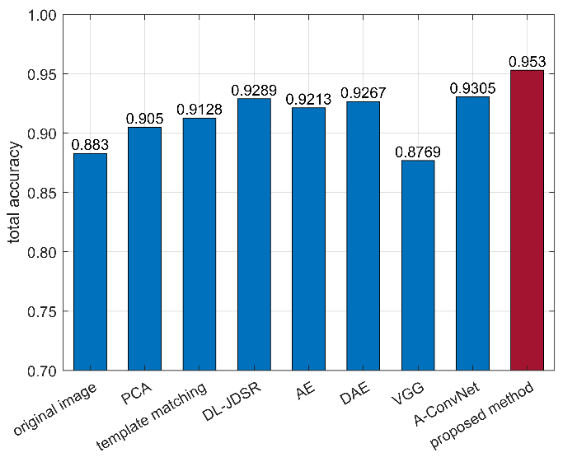
| Toyota Camery | Honda Civic 4dr | 1993 Jeep | 1999 Jeep | Nissan Maxima | Mazda MPV | Mitsu- Bishi | Nissan Sentra | Toyota Avalon | Toyota Tacoma | Total Accuracy | |
|---|---|---|---|---|---|---|---|---|---|---|---|
| Proposed method | 0.8694 | 0.9472 | 1 | 0.9306 | 0.9639 | 0.9528 | 0.9111 | 0.9889 | 1 | 0.9667 | 0.9530 |
| Original image | 0.9666 | 0.9306 | 0.9861 | 0.6528 | 0.7833 | 1 | 0.9 | 0.6111 | 1 | 1 | 0.8830 |
| PCA | 0.9444 | 0.9389 | 0.9556 | 0.6944 | 0.8278 | 1 | 0.9583 | 0.7306 | 1 | 1 | 0.9050 |
| Template matching | 0.9083 | 0.9194 | 0.9389 | 0.8722 | 0.9167 | 0.9444 | 0.8639 | 0.8333 | 0.9444 | 0.9861 | 0.9128 |
| DL-JDSR | 0.8833 | 0.9806 | 0.9750 | 0.9111 | 0.9639 | 0.8222 | 0.9583 | 0.9444 | 0.85 | 1 | 0.9289 |
| AE | 0.9944 | 0.9639 | 0.9389 | 0.8722 | 0.8778 | 0.9694 | 0.9639 | 0.6333 | 1 | 1 | 0.9213 |
| DAE | 0.9889 | 0.9722 | 0.9917 | 0.85 | 0.8833 | 0.9722 | 0.9278 | 0.6833 | 0.9972 | 1 | 0.9267 |
| VGGNet | 0.8278 | 0.7694 | 0.9611 | 0.7 | 0.9361 | 0.9139 | 0.8417 | 0.9194 | 0.9750 | 0.9250 | 0.8769 |
| A-ConvNets | 0.8694 | 0.9306 | 0.9972 | 0.8444 | 0.9917 | 0.9528 | 0.7306 | 0.9972 | 1 | 0.9917 | 0.9305 |
| ResNet-18 | 0.9452 | 0.9345 | 0.9764 | 0.8857 | 0.9248 | 0.9934 | 0.7756 | 0.7911 | 1 | 0.9847 | 0.9211 |
| ResNet-34 | 0.9437 | 0.9647 | 0.9713 | 0.6793 | 0.9537 | 0.9769 | 0.8985 | 0.8865 | 0.9691 | 1 | 0.9247 |
| DenseNet | 0.9608 | 0.9762 | 0.9842 | 0.9136 | 0.9157 | 0.9845 | 0.8223 | 0.7567 | 1 | 1 | 0.9314 |
| MBGH+CNN with EFF | 0.8757 | 0.9827 | 0.9801 | 0.8348 | 0.9214 | 0.9187 | 0.8467 | 0.8709 | 0.9422 | 0.9341 | 0.9017 |
Publisher’s Note: MDPI stays neutral with regard to jurisdictional claims in published maps and institutional affiliations. |
© 2021 by the authors. Licensee MDPI, Basel, Switzerland. This article is an open access article distributed under the terms and conditions of the Creative Commons Attribution (CC BY) license (https://creativecommons.org/licenses/by/4.0/).
Share and Cite
Du, L.; Li, L.; Guo, Y.; Wang, Y.; Ren, K.; Chen, J. Two-Stream Deep Fusion Network Based on VAE and CNN for Synthetic Aperture Radar Target Recognition. Remote Sens. 2021, 13, 4021. https://doi.org/10.3390/rs13204021
Du L, Li L, Guo Y, Wang Y, Ren K, Chen J. Two-Stream Deep Fusion Network Based on VAE and CNN for Synthetic Aperture Radar Target Recognition. Remote Sensing. 2021; 13(20):4021. https://doi.org/10.3390/rs13204021
Chicago/Turabian StyleDu, Lan, Lu Li, Yuchen Guo, Yan Wang, Ke Ren, and Jian Chen. 2021. "Two-Stream Deep Fusion Network Based on VAE and CNN for Synthetic Aperture Radar Target Recognition" Remote Sensing 13, no. 20: 4021. https://doi.org/10.3390/rs13204021
APA StyleDu, L., Li, L., Guo, Y., Wang, Y., Ren, K., & Chen, J. (2021). Two-Stream Deep Fusion Network Based on VAE and CNN for Synthetic Aperture Radar Target Recognition. Remote Sensing, 13(20), 4021. https://doi.org/10.3390/rs13204021