Abstract
Profile radar allows direct characterization of the vertical forest structure. Short-wavelength, such as Ku or X band, microwave data provide opportunities to detect the foliage. In order to exploit the potential of radar technology in forestry applications, a helicopter-borne Ku-band profile radar system, named Tomoradar, has been developed by the Finnish Geospatial Research Institute. However, how to use the profile radar waveforms to assess forest canopy parameters remains a challenge. In this study, we proposed a method by matching Tomoradar waveforms with simulated ones to estimate forest canopy leaf area index (LAI). Simulations were conducted by linking an individual tree-based forest gap model ZELIG and a three-dimension (3D) profile radar simulation model RAPID2. The ZELIG model simulated the parameters of potential local forest succession scene, and the RAPID2 model utilized the parameters to generate 3D virtual scenes and simulate waveforms based on Tomoradar configuration. The direct comparison of simulated and collected waveforms from Tomoradar could be carried out, which enabled the derivation of possible canopy LAI distribution corresponding to the Tomoradar waveform. A 600-m stripe of Tomoradar data (HH polarization) collected in the boreal forest at Evo in Finland was used as a test, which was divided into 60 plots with an interval of 10 m along the trajectory. The average waveform of each plot was employed to estimate the canopy LAI. Good results have been found in the waveform matching and the uncertainty of canopy LAI estimation. There were 95% of the plots with the mean relative overlapping rate (RO) above 0.7. The coefficients of variation of canopy LAI estimates were less than 0.20 in 80% of the plots. Compared to lidar-derived canopy effective LAI estimation, the coefficient of determination was 0.46, and the root mean square error (RMSE) was 1.81. This study established a bridge between the Ku band profile radar waveform and the forest canopy LAI by linking the RAPID2 and ZELIG model, presenting the uncertainty of forest canopy LAI estimation using Tomoradar. It is worth noting that since the difference of backscattering contribution is caused by both canopy structure and tree species, similar waveforms may correspond to different canopy LAI, inducing the uncertainty of canopy LAI estimation, which should be noticed in forest parameters estimation with empirical methods.
1. Introduction
Leaf area index (LAI), defined as half the total leaf area per unit of the horizontal ground surface area [1], is an essential indicator for forest ecosystem assessment and management. Forest LAI reflects the growth status of the forest. It is closely related to the photosynthesis, respiration, and transpiration of the forest [2]. LAI has been used as an input of ecological models and climate models as well [3,4,5]. Thus, forest LAI estimation plays a major role in forestry and ecology research. Remote sensing is generally utilized to retrieve forest LAI in large areas [2,6].
According to the different data types, the methods of estimating forest LAI using remote sensing technology fall into two main categories: optical data-based and lidar data-based. Optical remote sensing relates various vegetation indices (such as the normalized difference vegetation index (NDVI)) to the LAI of forest, which tends to have good performance for estimating forest LAI within a limited range of LAI values relative to saturation at high LAI level [2,7,8,9]. Lidar remote sensing provides detailed vertical structural information of forest canopy, which is contributed to estimate the LAI of forest canopy, and numerous studies have inversed forest canopy LAI utilizing lidar data [10,11,12]. Only a few studies have used microwave data to estimate forest LAI. The initial research began with microwave backscattering indoor-measurement of miniaturized forest scene [13], which pointed out that the short wavelength radar signals, such as X and C band, are sensitive to the changes of tree leaf area. Based on C band environmental satellite (ENVISAT) advanced synthetic aperture radar (ASAR) data and LAI ground measurements, Manninen et al. conducted LAI estimation of the boreal forest in Finland in 2005 [14] and 2013 [15], respectively, using the empirical model. Tanase et al. (2019) utilized the physical model simulation to prove once again that the C band microwave signal can respond to the changes of forest LAI and have the potential to estimate forest LAI [16]. Recently, a novel Ku-band profile radar system [17], named Tomoradar, was developed by the Finnish Geospatial Research Institute (FGI) based on early bird work [18,19,20], which has obvious advantages in forest structure mapping. Compared to optical data, the Tomoradar signal can penetrate through the forest canopy and provide entire profile information from canopy top to ground level. Compared to lidar data, the Tomoradar signal has a more substantial penetration capability within the forest [21], which means that the accurate vertical forest structure can be obtained with the Tomoradar waveform. Moreover, compared to synthetic aperture radar tomography (TomoSAR), the Tomoradar data have a higher vertical resolution (0.15 m) and intuitive scatterer contribution. In addition, Du et al. have shown that the waveforms of Tomoradar are sensitive to foliage volume [22]. To this end, the Tomoradar data exhibit excellent potential in the LAI estimation of forest canopy.
However, how to take advantage of Tomoradar data to estimate forest canopy LAI? Using the idea of retrieving LAI from full-waveform lidar for reference, two methods could be applied to Tomoradar data to estimate the LAI of forest canopy. One reference method is to apply Beer–Lambert law, which calculates the ratio of light intensity between the bottom and top of the forest canopy, and combines the observed LAI data to construct a semi-empirical model for LAI estimation [23]. In 2018, Zhu utilized Tomoradar data to estimate canopy LAI by regarding the ratio of light intensity as the ratio of the ground backscattering energy to the total backscattering energy and ignoring the reflectance difference between the ground and various tree species [24]. The other reference method is the waveform matching method based on a physical model. The physical model characterizes the interaction between vegetation elements and electromagnetic waves, and by simulating the response of the forest canopy with different attributes, various simulated waveforms are obtained to match the observed waveform, acquiring possible forest attributes distribution. Rödig et al. (2019) utilized a forest gap model, the FORMIND model, and its built-in lidar simulation module to simulate the Geoscience Laser Altimeter System (GLAS) lidar waveform, and estimated the five kinds of key forest attributes in the entire Amazon [25]. Compared with the semi-empirical model-based method, the waveform matching method based on the physical model can obtain the possible distribution range of the estimated forest attributes rather than a single estimation result. In addition, the method does not require extensive field inventories.
Considering that the quantitative relationship between the Ku band profile radar waveform and the forest canopy parameters is not clear, the aim of this work is to explore the ability of using Tomoradar waveform to estimate forest canopy LAI by utilizing the waveform matching method based on the radiative transfer model. This method can obtain not only the estimated value of the forest canopy LAI, but also the corresponding uncertainty, which helps to analyze the source of the error in the LAI estimation based on profile radar data, so as to further improve the accuracy of forest canopy LAI estimation in the future.
2. Material and Methods
2.1. Study Site and Data Collection
This study was carried out at Evo, located in the boreal forest region in southern Finland (61°19′N, 25°11′E) as shown in Figure 1a. About 2000 ha of half-managed forest is mainly covered by Scots pine (Pinus sylvestris), Norway spruce (Picea abies), and birch (Betula sp.) in this area. The study site has a relatively flat landscape and temperate maritime climate. Its annual average temperature and cumulative precipitation are 4.1 °C and 635 mm, respectively [26,27]. The Tomoradar data were collected by a Bell-206 helicopter at the Evo site in September 2016, which operated at around 60–100 m altitude with an average 10 m/s flight speed on a trajectory with a total length of 60 km. In this research, one stripe with a length of 600 m along a north-south direction flight trajectory was utilized to estimate forest canopy LAI (presented in Figure 1b), which covered area with different forest density and tree height. Another reason we selected the stripe is that the directional flight can ensure the observation angle in the nadir direction, which is conducive to data quality [28].
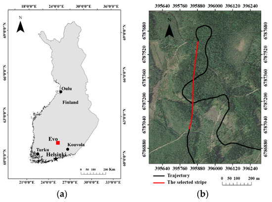
Figure 1.
(a) Location of the study area (Evo) in southern Finland; (b) trajectory of Tomoradar data (black line) and the selected 600 m stripe (red line), in addition, the base map employed an image provided by Google Earth with a resolution of 0.5 m to show the forest condition.
2.2. Tomoradar Data
The airborne Tomoradar system is a frequency modulated continuous wave (FM-CW) ranging radar with a global navigation satellite system (GNSS) and inertial measurement unit (IMU) system, which provide centimeter-level accuracy of flight trajectory information. Tomoradar works in the Ku-band with a center frequency 14 GHz and a modulation frequency 163 Hz. Tomoradar can collect four polarization modes (HH, HV, VH, and VV) signal within the field of view (FOV) of 6°, and convert them into waveforms with a 0.15 m range resolution. Due to the average flight speed of the helicopter being 10 m/s, the spacing between two consecutive/neighboring waveforms along trajectory was 0.06 m. Since the mechanical scanner was not equipped, the observation angle of Tomoradar is only in the nadir direction along the flight trajectory. Moreover, the footprint size of a single waveform is determined by the flight altitude and the FOV. The main parameters of Tomoradar are shown in Table 1. More detailed technical characteristic information of Tomoradar can be obtained by Chen et al. [17].

Table 1.
Main parameters of Tomoradar. FM-CW: frequency modulated continuous wave.
The selected stripe with a length of 600 m contains 10002 Tomoradar waveforms in co-polarization (HH) mode, which were employed to estimate the forest canopy LAI. In the stripe, the range of flight height was between 58 and 71 m, which determined the footprint width was varied from 6.1 to 7.5 m at the ground. The vertical profile of the backscattering energy of the stripe in HH polarization mode is illustrated in Figure 2. Considering the average footprint width of 6.8 m and the interval of 0.06 m between two neighbor footprints centers, there is a certain degree of duplicate information in 10,002 waveforms. To this end, we divided the 600 m stripe into 60 plots at an interval of 10 m along the trajectory, and calculated the average waveform of each plot to estimate the forest canopy LAI.
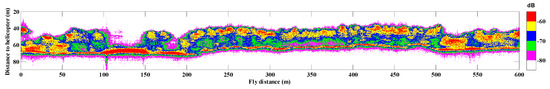
Figure 2.
The Tomoradar vertical profile of the selected 600 m stripe in co-polarization (HH) mode is colored with backscattering energy intensity.
2.3. Lidar Data
For reference, a lidar-derived canopy effective leaf area index (LAIe) estimation was used in this study. The lidar data were obtained simultaneously with Tomoradar data, collected by a Velodyne VLP-16 laser scanner installed on the same helicopter-borne platform [17]. It works with 300,000 pts/s, generates 16 scan lines uniformly, and the beam size of the transmitted laser pulse at the exit is 12.7 mm (horizontal) × 9.5 mm (vertical). The main parameters of the lidar system are presented in Table 2. For the selected stripe, the lidar data were collected with an average point density of about 85 pts/m2.
Table 2.
Main parameters of the lidar system.
2.4. Forest Canopy LAI Estimation by Waveform Matching
The Tomoradar waveform depicts the vertical distribution of backscattering energy from the canopy top to the ground. Since the Ku-band is sensitive to foliage [22], the potential of the Tomoradar waveform to estimate forest canopy LAI was explored in this study. Here, we proposed a method by matching Tomoradar waveform with the simulated waveforms acquired by forest succession simulation and profile radar waveform simulation to estimate canopy LAI (Figure 3). Specifically, 100-year succession process after the clear cutting at Evo was simulated with the ZELIG model, and the information of 10,000 virtual forest scenes was obtained (introduced in Section 2.4.1). Then, based on the information of each scene, the 3D scene reconstruction and the waveform simulation were completed in RAPID2 (introduced in Section 2.4.2). Moreover, considering the heterogeneity of ground, 4 coefficients were set to extend various ground contribution in the simulated waveform, and summing up to 50,000 simulated waveforms were utilized to waveform matching. In addition, by matching the average Tomoradar waveform of each plot with simulated waveforms, the probability distribution of forest canopy LAI could be derived with the top 30 best matches (introduced in Section 2.4.3).
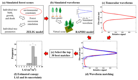
Figure 3.
Workflow of this study. (a) using the ZELIG model to simulate the 100-year succession process and individual tree parameters after the clear cutting at Evo; (b) using RAPID2 to simulate the 3D scene and the waveform; (c) calculating the average Tomoradar waveform of each plot; (d) matching the average Tomoradar waveform with simulated waveforms for each plot; (e) selecting the top 30 best matches in all simulated waveforms for each plot; (f) estimating the canopy leaf area index (LAI) and its uncertainty based on the selected simulated waveforms.
2.4.1. Forest Gap Model and Forest Succession Simulation
Forest gap model is a type of forest dynamic model based on the forest gap succession theory, which can simulate the process of tree regeneration, growth, and death within a forest gap. In this study, the ZELIG model, an individual tree-based forest gap model, was used to generate forest scenes [29]. ZELIG was derived from the JABOWA and FORET model [30,31], and has been widely applied in forest parameter estimation by combining a three-dimension radiative transfer (RT) model [32,33,34]. ZELIG is based on a grid of 10 m × 10 m cells, in which each tree is assigned to a certain cell, and the grid dimensions are users-defined. Annual regeneration, growth, and mortality of individual trees on each cell can be interactively simulated in response to their biophysical parameters and environmental constraints. The biophysical parameters of each species mainly include the maximum age (Amax), maximum diameter at breast height (Dmax), maximum height (Hmax), growth rate (G), minimum and maximum growing degree-days (DDmin, DDmax), and tolerance class for shade (Light), drought (Drt), and soil fertility (Nutri). When it comes to environmental data, monthly average temperature and cumulative precipitation are the main inputs for the ZELIG model. After simulation, the annual forestry parameters of each individual tree are provided by the ZELIG model, including species, diameter at breast height (DBH), height, crown length, and leaf area, etc.
In this study, we simulated a 100-year succession process of a 10 m × 10 m plot with a 2-year interval by ZELIG model. The simulation starts after the clear cutting, and the simulated species include Scots pine, Norway spruce, and birch, which are the dominant species at Evo. Considering the random processes in the ZELIG model, 200 repetitions were implemented for each of the time steps to obtain the plot scenes that contain as many situations as possible. These sum up to 10,000 simulated plots in total. In addition, in order to properly work with the RAPID2 model for plot scene construction, a random coordinate within the cell of each tree was assigned as it is generated in the ZELIG model, and it will be fixed until the tree is dead. Finally, the individual tree parameters within the plot provided by the ZELIG model include the locations, DBH, heights, crown length, and leaf area, which were used as inputs to generate the 3D forest scenes required in the RAPID2 model.
The specific biophysical parameters of the three dominant tree species are shown in Table 3 [31,35]. The monthly average temperature and cumulative precipitation at Evo were calculated by GHCN_CAMS Gridded 2m Temperature (Land) (1948–2019) [26] and CPC Merged Analysis of Precipitation (CMAP) (1979–2019) [27], respectively.
Table 3.
Specific biophysical parameters of the three dominant tree species provided to the ZELIG model.
2.4.2. RAPID2 Model and Waveform Simulation
The RAPID2 model is a 3D RT model by proposing the concept of porous individual thin objects, developed by Huang et al. [36], which simulates the radiation transfer from visible/near infrared to thermal infrared and microwave domain with a unified 3D scene and input parameters. Users can generate a forest scene with the built-in 3D scene graphical user interface (GUI) and simulate remote sensing data with a unified radiosity framework. The RAPID2 model is freely shared online (http://www.3dforest.cn/en_rapid.html). The purpose of the RAPID2 model in this research is to simulate profile radar waveforms of a given forest scene provided by the ZELIG model.
The inputs of the RAPID2 model can be divided into two parts: scene generation parameters and sensor simulation parameters. The scene generation parameters mainly include the size and the digital elevation model (DEM) of the scene, soil parameters (roughness size and correlation length), as well as 3D objects (such as trees) parameters in the scene. Sensor simulation parameters consist of observation angle, wavelength, and resolution, etc. For the tree object, users can describe it through individual tree parameters, crown shape parameters, and crown structure parameters. The individual tree parameters include location, species, DBH, height, crown length, crown width, and leaf area. The built-in crown shape mainly involves spherical, conical, cylindrical, and other basic shapes. The crown structure parameters are composed of leaves (needles) parameters and branches parameters, embodied in length, thickness, orientation and length, diameter, density, respectively. The branches are divided into large branches and small twigs. In addition, in the microwave domain, the dielectric constants of leaf, branch, stem, and soil need to be defined with environment moisture and temperature, which play an important role for their scattering and extinction characteristics.
Recently, Du et al. realized the simulation of the profile radar waveform by extending the RAPID2 model, and confirmed that the Ku-band profile radar is sensitive to the individual tree LAI [22], which reflects the great potential of using the Ku-band profile radar to estimate forest canopy LAI. A sample forest scene in RAPID2 and its approximate profile radar waveform simulation are presented in Figure 4.
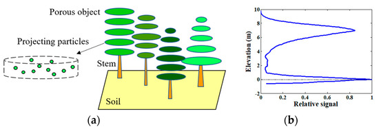
Figure 4.
(a) A sample forest scene in the RAPID2 model, which is composed of soil, solid stems, and porous crowns; the porous crowns consist of many thin layers, which are projected as particles dynamically in microwave domain at runtime; (b) an approximate profile radar waveform simulation of the scene.
In order to construct the 3D scenes of the virtual plot scenes in the RAPID2 model and make the scenes more realistic, some crown shape and structure parameters, as well as the dielectric constants, etc. were defined here.
First of all, the crown shape parameters of the three species were determined according to the literature [37]: the crown shape of the Scots pine and Norway spruce can be represented using two conical elements, while that of the birch can be represented using an obloid and a hemisphere elements. The specific details were described by the maximum crown radius (Cr), the height of Cr (HCr), and the bottom crown radius (Rc), which were related to the DBH, tree height (H), and crown length (Cl). The allometric relationships of the three species are listed in Table 4.
Table 4.
The allometric relationships of Scots pine, Norway spruce, and birch.
Then, the crown structure parameters, such as leaves (needles) and branches parameters, were mainly referenced in the literature [22]. The leaves (needles) parameters were set by species, while the branch parameters were uniform for all three species, as shown in Table 5. The leaf angle distribution (LAD) and branch orientation distribution (BOD) were set from 0° to 85° with a step of 5°, assumed to be independent of azimuth.
Table 5.
The main crown structure parameters of the three species for simulation.
Moreover, the dielectric constants of scene components in Ku-band were calculated according to Ulaby [38] in this study, which did not distinguish between species (Table 6). In addition, the flat terrain was adopted for the 10 m × 10 m scene. The soil roughness height and correlation length were set to be 0.25 and 18.75 cm, respectively.
Table 6.
The dielectric constants of scene components in Ku-band.
To sum up, the 3D scenes of the plots provided by ZELIG were constructed in the RAPID2 model utilizing the parameters described above. The individual tree model of the three species and a 50-year-old plot scene in the RAPID2 model are illustrated in Figure 5.
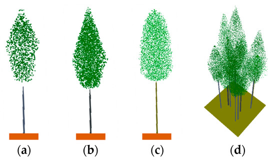
Figure 5.
The individual tree model of the three species and a 50-year-old plot scene in the RAPID2 model: (a) Scots pine; (b) Norway spruce; (c) birch; and (d) a 50-year-old plot scene.
With the 3D scenes of the 10,000 plots as inputs, 10,000 profile radar waveforms were generated using the RAPID2 model. For matching the collected Tomoradar waveforms, the Tomoradar configuration was adopted in the waveform simulation, specifically the nadir observation angle, the operating frequency of 14 GHz, the range resolution of 0.15 m, and the footprint-width of 6.8 m. Considering the data redundancy caused by the high azimuth sampling frequency (0.06 m), it was modified to 1 m in the simulation process.
2.4.3. Waveform Matching and Canopy LAI Estimation
We compared each Tomoradar average waveform with the simulated profile radar waveforms using the waveform matching method [39]. The ground points of both Tomoradar waveforms and simulated waveforms were identified firstly [28] and the range from the ground point to 2 m above the ground point was treated as ground scattering contribution [21]. In order to correspond to the difference in ground scattering intensity caused by possible ground features (such as different ground cover, moisture, or micro-topography) in the actual scenes, we performed differential amplification on the ground scattering contribution of the simulated waveform, that is, the ground contribution was multiplied by four coefficients of 0.1, 0.4, 0.7, and 1.3. Therefore, the number of simulated waveforms was increased from 10,000 to 50,000, which is conducive to cover the complex actual situation of the plots.
During the comparison, the similarities of normalized (by the max intensity including ground scattering) Tomoradar and simulated waveforms were determined by quantifying their relative overlapping rate (RO) in each 1 m height bin above 2 m, which was calculated by the intersection area divided by union area [39], Equation (1):
where the RO is the relative overlapping rate of the Tomoradar waveform and simulated waveform; ETomo(h) and Esimu(h) are the relative energy at height “h” of the Tomoradar waveform and simulated waveform, respectively; the height step is set to 1 m.
The top 30 best matching simulated waveforms with the RO above the threshold of 70%, as acceptable waveforms, were adopted to identify potential plot scenes and acquire their canopy LAI attribute [25]. If the number of acceptable waveforms is less than 30, only the waveforms with the RO above the threshold were taken. Additionally, when the number of acceptable waveforms is less than 3, the top 3 matches were taken. Hence, we derived a series of possible canopy LAI from the workflow for each Tomoradar waveform. The estimated canopy LAI of the plot was defined as the mean value of the possible canopy LAI, while its uncertainty was defined as the coefficient of variation (CV) of the possible canopy LAI. The mean canopy height (MCH) was utilized to represent the vertical structure of the actual plots, expressed as Equation (2), and it was used to analyze the possible difference in estimation results:
In addition, the lidar-derived canopy effective LAI was used to reference the estimated canopy LAI of our approach. According to the Tomoradar waveforms contained in each plot, the lidar points inside the Tomoradar footprint cone were used to calculate the lidar-derived canopy LAI. Based on Beer–Lambert law, the canopy LAI of the plots can be determined by the light intensity at the top and bottom of the canopy and the corresponding extinction coefficient [23]. For lidar point cloud data, the light intensity at the top of the canopy can be regarded as the total number of reflected laser points from the full scene, and the bottom light intensity is regarded as the number of reflected laser points from the part below 2 m above the ground (corresponds to Tomoradar). Thus, the lidar-derived canopy effective LAI of each plot was obtained by Equation (3) [40]:
where Rg is the number of reflected laser points from the part below 2 m above the ground and Rt is the total number of reflected laser points from the full scene.
3. Results
3.1. Forest Scenes Simulation
The forest scenes simulation at different succession stages can reproduce the canopy LAI (actual LAI) changing over time. Using the ZELIG model and corresponding local parameterization as mentioned above, the canopy LAI distribution of the simulated 10,000 plots is presented in Figure 6.
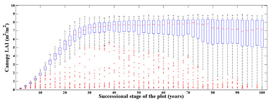
Figure 6.
The canopy actual LAI distribution of the simulated 10,000 plots. There are 200 plots for each succession stage over 100 years with an interval of 2 years. The red lines represent the median of the LAI distribution; the blue rectangles represent the upper and lower quartile interval; the black dashed lines represent the upper and lower limits; and the red dots represent the outliers of the LAI distribution.
Figure 6 demonstrates the process that the canopy LAI of the simulated plots increased rapidly over time and finally stabilized. Further, their distribution range was from close to 0 to about 9.0. Specifically, for the first 30 years of the succession from the bare ground, the canopy LAI of the simulated plots presented a logistic growth pattern, and the median of the canopy LAI distribution was stable at around 7.0. During this period, the 200 plots at each succession stage had a relatively unified canopy LAI distribution. For the 30 to 100 years of succession, the median of the canopy LAI distribution was still about 7.0 at each stage, however, the canopy LAI distribution at the same succession stage tends to be dispersed, which was determined by the random process in the death and regeneration module of the individual tree in the ZELIG model. In general, the canopy LAI distribution of the 10,000 simulated plots basically covered the possible canopy LAI at Evo, which met the needs of our approach to estimate the canopy LAI.
3.2. The Relative Overlapping Rate and Uncertainty
The Tomoradar average waveform of each plot was compared with the 50,000 simulated waveforms to determine the potential plot scenes and corresponding canopy LAI attributes. The matching degree of the acceptable waveforms over 2 m above ground and the uncertainty of the estimated canopy LAI of two example plots are illustrated in Figure 7, which contained the best matching simulated waveform, the range of the top 30 best matching simulated waveforms, as well as their corresponding canopy LAI and their coefficients of variation. Figure 7 shows that, for some plots, the acceptable waveforms had high relative overlapping rate with Tomoradar waveform, and revealed a clear forest scene for which simulated canopy LAI differ slightly (Figure 7a,b). On the other hand, the acceptable waveforms for other plots, of which the RO was insufficient, showed ambiguities in canopy LAI estimation (Figure 7c,d).
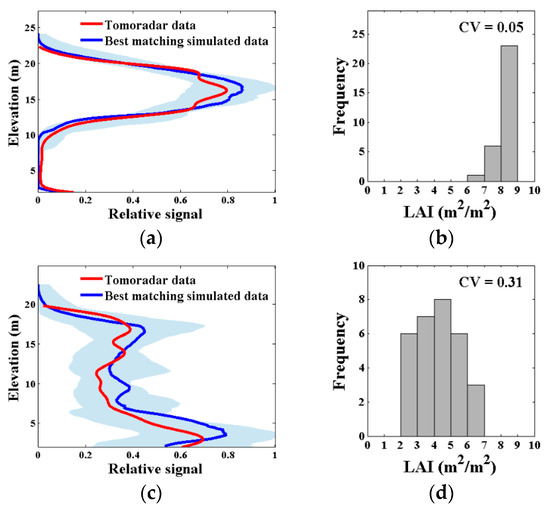
Figure 7.
The matching degree of the acceptable waveforms over 2 m above ground and the uncertainty of the estimated canopy LAI of two example plots. (a,c) The Tomoradar average waveform (red), the best matching simulated waveform (blue), and the range of all acceptable waveforms (light bule); the relative overlapping rate (RO) of all acceptable waveforms in (a,c) were > 80% and > 70%, respectively; (b,d) the estimated canopy LAI distribution for all acceptable waveforms and their coefficients of variation (CV), defined as uncertainty.
The mean RO of the acceptable waveforms was utilized to characterize the matching degree in the plot. The mean RO of the acceptable waveforms of all 60 plots is presented in Figure 8a. An analysis has shown that the number of plots where the mean RO of the acceptable waveforms reaching the threshold (0.7) accounted for 95% of the total plots. There were 44 plots with a mean RO between 0.7 and 0.8 in this simulation, which was the largest proportion. Figure 8b shows the distribution of the coefficients of variation of canopy LAI estimation for all 60 plots. There were 48 plots with a coefficient of variation lower than 0.20, accounting for 80% of all plots, which presented the low uncertainty of the canopy LAI estimation in this research. In addition, the coefficients of variation were more concentrated in two intervals of 0.05 to 0.10 and 0.10 to 0.15, which contained 23 plots and 12 plots, respectively.

Figure 8.
(a) The mean relative overlapping rate (RO) distribution of the acceptable waveforms and (b) the coefficients of variation of canopy LAI estimation for all 60 plots.
In addition, the relationship between the mean RO and uncertainties for all plots are shown in Figure 9. In order to reflect the possible differences caused by the characteristics of plot scenes and the number of matching waveforms, the mean canopy height (MCH) and the number of acceptable waveforms of each plot were used in the mapping.
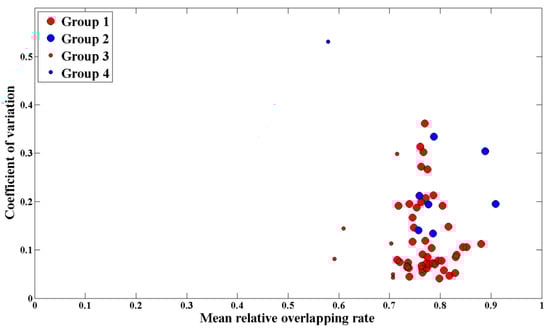
Figure 9.
The relationship between the mean RO and uncertainties for all plots. The red dots represent plots with the mean canopy height (MCH) greater than or equal to 5 m, while the blue dots represent plots with an MCH less than 5 m. The larger dots mean that the number of acceptable waveforms reached 30 in the matching process, while the smaller dots mean that the number was less than 30.
Figure 9 shows that there is no clear correlation between the mean RO of plot and the canopy LAI estimation uncertainty (p = 0.25). However, the waveform matching degree and the uncertainty of canopy LAI estimation presents promising results, respectively. The mean RO of the plot was higher than 0.70 in general, and the coefficient of variation of estimated canopy LAI was less than 0.20 for the most part of plots. Specifically, compared with most plots with higher MCH, the only 8 plots with an MCH of less than 5 m showed bigger uncertainty in canopy LAI estimation, even though the waveform matching performed well. For 7 plots with less than 30 acceptable waveforms, there were poorly waveform matching, but the coefficients of variation of 5 plots were less than 0.20.
3.3. Canopy LAI Estimation
Based on the waveform matching, the canopy LAI of each plot was determined by the mean value of the possible canopy LAI. The distribution of the estimated canopy LAI of all 60 plots is shown in Figure 10a, and the corresponding estimation uncertainty distribution is shown in Figure 10b.
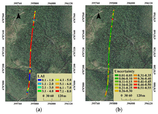
Figure 10.
(a) The distribution of the estimated canopy LAI of all 60 plots, and (b) the corresponding estimation uncertainty distribution.
The general distribution of canopy LAI was that the high canopy LAI (6.1 to 8.0) was concentrated mainly on the dense forest zone in the middle of the selected stripe, while the approximate non-forestland located in the south had an estimate less than 1.0 (Figure 10a). For the distribution of uncertainty as shown in Figure 10b, the coefficients of variation in the middle of the selected stripe were less than 0.20, however, in the forest zone with low LAI located in the south and north, the coefficients of variation were relatively high, especially in the areas with an estimated canopy LAI less than 2.0.
The estimated canopy LAI derived from Tomoradar was compared with lidar-derived canopy LAI estimates for each plot. Their relationship was investigated, and the scatter plot is illustrated in Figure 11.
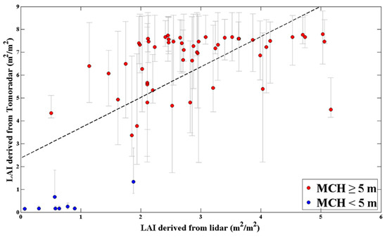
Figure 11.
The relationship between the Tomoradar-derived and lidar-derived canopy LAI estimates. The red dots represent the plot with an MCH greater than or equal to 5 m, while the blue dots represent the plot with an MCH less than 5 m. The error bars for the Tomoradar-derived canopy LAI estimates (vertical grey error bars) come from the ranges of corresponding canopy LAI of all acceptable waveforms. The dashed line is the regression line: y = 1.33x + 2.368; R2 = 0.46; root mean square error (RMSE) = 1.81.
Figure 11 shows that compared with the lidar-derived estimation result, the Tomoradar-derived canopy LAI estimates were higher. The Tomoradar-derived canopy LAI estimates were mostly distributed between 7.0 and 8.0, and another part was concentrated around 5.0, while the lidar-derived estimation result was distributed between 2.0 and 5.0, and the value between 2.0 and 3.0 accounted for more. There were 8 plots with an MCH of less than 5 m, of which the estimated canopy LAI was less than 2.0 for both Tomoradar-derived and lidar-derived. The coefficient of determination between the Tomoradar-derived canopy LAI estimates and that of lidar-derived was 0.46, and the root mean square error (RMSE) was 1.81.
4. Discussion
This study demonstrated an approach for estimating the canopy LAI using Ku-band profile radar waveforms with the waveform matching method based on linking the 3D RT model RAPID2 and forest gap model ZELIG. By calculating the relative overlapping rate between the observed and simulated waveforms, the top 30 best matching simulated waveforms with RO above the threshold of 0.7, as acceptable waveforms, were employed to acquire possible canopy LAI. The matching degree of the acceptable simulated waveforms, the probability distribution of forest canopy LAI, and the final canopy LAI estimation results were explored. In the following section, we discuss the results in detail, as well as the advantages and limitations of the approach.
4.1. Uncertainty of the Canopy LAI Estimation
The uncertainty of the canopy LAI estimation is mainly discussed from three aspects, the relationship between waveform matching degree and the uncertainty, the relationship between canopy LAI level of plots and the uncertainty, as well as the divergence of canopy LAI estimation results between Tomoradar-derived and lidar-derived.
Figure 9 shows an ambiguous relationship between the mean RO and the canopy LAI estimation uncertainty, even if they had good performance separately. As the mean RO of plots increased, the uncertainty of canopy LAI estimation did not present a downward trend. Especially for plots with a mean RO between 0.7 and 0.8, their uncertainties were discretely distributed between 0.04 and 0.40, and mostly concentrated below 0.20. To our knowledge, a similar situation arises in a previous study using full-waveform lidar to estimate the biomass in the Amazon rainforest [25]. In the lidar waveform matching process, the mean RO was generally greater than 0.70, and the coefficient of variation of estimated forest aboveground biomass was about 0.2. However, for some plots, the estimated aboveground biomass values differ, while the simulated waveforms are similar. They proposed that due to different species with various wood densities, the forest aboveground biomass values may not be consistent, although there are trees with the same shape and size in the scene. Similarly, for scenes with the same Ku-band response, they may still correspond to different canopy LAI, considering that the various leaf parameters of different species lead to different scattering contribution. Thus, there is no strict relationship between the mean RO and the canopy LAI estimation uncertainty.
For the distribution of the canopy LAI estimation uncertainty, an uncommon situation is that the uncertainty was lower in plots with high canopy LAI level, but higher in plots with thin forest stand, as shown in Figure 10. This is, to some extent, due to the uncertainty expressed as the coefficient of variation of estimated canopy LAI. The coefficient of variation is obtained by dividing the standard deviation of the observations by the mean value. When the estimated canopy LAI is close to 0, a small disturbance will cause a huge impact on the coefficient of variation. In response to this problem, another evaluation index, the quartile coefficient of dispersion (QC), was used to express the uncertainty. The distribution of quartile coefficient of dispersion for all 60 plots canopy LAI estimation is presented in Figure 12a, and the corresponding uncertainty (QC) distribution in the selected stripe is presented in Figure 12b.
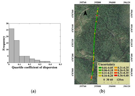
Figure 12.
(a) The distribution of quartile coefficient of dispersion for all 60 plots canopy LAI estimation and (b) the corresponding uncertainty (QC) distribution of canopy LAI estimation.
We find that there were 53 plots with the quartile coefficient of dispersion of less than 0.20 for all 60 plots canopy LAI estimation (Figure 12a), which proves the low uncertainty of canopy LAI estimation in this study. For the uncertainty distribution, the QC-expressed uncertainty distribution is similar to that of the CV-expressed (Figure 12b). Compared to the higher CV-expressed uncertainty in the thin forest plot, the QC-expressed uncertainty is reduced to a certain extent, by eliminating the self-influence of the canopy LAI estimates level on the uncertainty evaluation. However, the thin forest plot with the higher uncertainty canopy LAI estimation still exists. This phenomenon could be related to the variation of tree species. The thin low-canopy-LAI plots mainly match the early succession scene, which contains more various tree species composition in most cases than that of the late succession scene. Considering that the scattering contributions of different tree species are distinctive, the plots composed of different tree species may obtain similar waveforms. Therefore, the thin forest plot presented the relative higher uncertainty of canopy LAI estimation.
Figure 11 illustrates the relationship between the Tomoradar-derived canopy LAI estimates and that of the lidar-derived. Compared to the lidar-derived estimates, the higher canopy LAI estimates were acquired with Tomoradar in this study. The possible reasons for the difference were analyzed from two aspects. One, for the Tomoradar-derived canopy LAI, the forest gap model ZELIG generates the forest scenes with actual LAI, which leads to the actual LAI obtained by the waveform matching method, while the lidar-derived LAI estimates are the effective LAI [40], which are often smaller than the actual LAI [41]. Two, since Tomoradar has stronger penetration than lidar [21], Tomoradar has more opportunities to gain the completed canopy LAI.
4.2. Comparison of Accuracy in Canopy LAI Estimation
To our knowledge, there are very few studies on deriving LAI from profile radar data. Zhu (2018) used Tomoradar data to estimate the canopy LAI based on Beer–Lambert law, and analyzed its relationship with lidar-derived LAI, but specific LAI value was not given [24]. In the estimation process, Zhu ignored the reflectance difference between the ground and various tree species at Ku band and the difference of the extinction coefficient in forest canopy between the Tomoradar signal and lidar signal. As a result, the Tomoradar-derived LAI was in good agreement with the lidar-derived LAI, the coefficient of determination was 0.65, and the RMSE was 0.098. However, combined with the finding of this research, the difference of backscattering contributions between the ground and various tree species has an evident impact on canopy LAI estimation, which should be noticed in future studies with semi-empirical methods. Although the actual canopy LAI in the selected stripe cannot be acquired as the reference in this study due to lack of ground measurements, our findings are meaningful and supplement to the forestry application of Tomoradar data.
To be general, a few studies on forest canopy LAI estimation using SAR data are also used for comparison. Manninen et al. (2005) utilized linear regression to complete the LAI estimation of boreal forest in central Finland using C band ENVISAT ASAR data [14]. In their study, the VV/HH polarization ratio had a good correlation with the LAI ground measurements, and the mean LAI estimation error was 0.3 for Norway spruce dominated plots, 0.07 for Scots pine dominated plots, and 0.27 for mixed forest plots. In 2013, their team employed a large amount of ENVISAT ASAR data and plot data to further analyze the linear regression relationship in the boreal and subarctic area [15]. They found out that a large observation angle is conducive to LAI estimation for side-looking radar. By increasing the number of pixels in the average backscattering process, the LAI estimation error tends to decrease exponentially. When high spatial resolution LAI estimation is required, more multi-temporal images covering the same area could reduce the LAI estimation error. Comparing the above-mentioned studies, it is important to emphasize the differences in methodology, although the estimation accuracy is lower (the RMSE was 1.81) in this study due to the reasons discussed in Section 4.1. By linking the forest gap model and the radiative transfer model, we explored the potential canopy LAI distribution of similar waveforms, and gave the estimated value of canopy LAI and the corresponding uncertainty, instead of regression results based on existing data. Clarifying the source of uncertainty in the estimation process will help the establishment of semi-empirical models with better estimation accuracy in the future. In addition, the uncertainty of the potential canopy LAI distribution is satisfactory in this study.
4.3. Advantage of the Approach
The current study has several advantages in terms of estimating canopy LAI with profile radar waveform. First, the differences of backscattering coefficients between the forest canopy and the ground and between different tree species were considered in the canopy LAI estimation process. The different backscattering coefficient means different backscattering energy contribution, which has an evident impact on forest parameters estimation. In previous studies, these differences are often assumed to be non-existent, especially for the difference between tree species.
Second, the entire Tomoradar waveforms were employed to quantify the canopy LAI. Compared with various Tomoradar metrics, such as forest height and backscattering energy quantile height, the entire waveform information shows the vertical heterogeneity of canopy LAI comprehensively and intuitively. By matching Tomoradar waveform with simulated waveforms, the similar simulated waveforms and the corresponding canopy LAI are obtained, which puts forward new ideas for canopy LAI estimation, instead of relying on a specific formula traditionally.
Third, the range of potential canopy LAI and the corresponding uncertainty can be determined by our approach. In previous studies, remote sensing metrics are often combined with the ground measurement. The parameter estimation is carried out by establishing a statistical relationship, which is not beneficial for estimating the uncertainty. Utilizing the combination of the RAPID2 model and ZELIG model, a large amount of plot scenes with various structures and their simulated waveforms are generated. For the similar waveform, the canopy LAI value of the plot may differ, since different tree species composition means different leaf backscattering contribution. The tree species-caused uncertainty of canopy LAI estimation could be presented by the approach. In the future, this understanding of Tomoradar waveform may be helpful for forest parameter estimation based on semi-empirical models.
Fourth, our approach is not limited to the size and quantity of ground inventory plots, and applications at different spatial scales can be carried out by selecting appropriate profile radar data and forest gap models. According to the characteristics of the Tomoradar data in this study, the ZELIG model, simulating the forest dynamic at the individual tree level in a 10 m × 10 m plot, was employed, which provided the complex vertical forest structure change under a long-term period. When Tomoradar collects data on a large scale in the future, the combination of the FORMIND model and RAPID2 model is also a good choice, which is widely used in large-scale forest parameter estimation based on large-footprint lidar data [25,39,42].
4.4. Limitation of the Approach
Despite the strengths of the approach, there are also some limitations. One shortcoming appears in forest scenes simulation with the ZELIG model. Although this research considers the growth, death, and regeneration on the individual tree level, as well as the environmental constrains and the interaction between the individual, the simplification and the uncertainty of environmental parameters exist in the ZELIG model, like every forest gap model. Further, compared to the plot with the size of 1 or 0.16 km2 in large-scale parameter estimation [25,39], the size of the plot in this study is only 100 m2. The smaller the scene, the greater the distortion may exist between the simulated and actual scenes, because the average effect is more obvious in the large scene [39]. It is probably that there are forest structure differences between simulated succession stage and actual succession stage in the study area. However, we do not pay attention to the specific succession stage of the scene. We believe that if enough scenes with various canopy LAI distribution are generated, which could include the canopy LAI distribution in natural scenes, we have the opportunity to estimate the canopy LAI accurately. In fact, for more than 95% of the actual plots, the relative overlapping rate between the acceptable simulated waveform and the Tomoradar waveform is greater than 0.7, and the canopy LAI estimation uncertainty of most of them is less than 0.20.
Another shortcoming appears in waveform simulation with the RAPID2 model. A primary problem in the application of 3D radiative transfer is that a large amount of inputs are required to describe the scene. Although the forest gap model ZELIG provides individual tree parameters, such as DBH, height, crown length, and leaf area, etc., more detailed canopy parameters (such as branches and twigs) and the dielectric constants of each component are set according to previous studies. It is possible that the errors of individual tree backscattering contribution may lead to inaccurate waveform simulation. However, it is difficult to measure the numerous parameters of canopy accurately even though ground inventory could be applied. On the other hand, the applied canopy parameters were used with the Tomoradar waveform simulation at Evo in the previous study, and a good simulation was achieved [22]. Hence, we assume that the inputs of waveform simulation are reliable, to some extent, and the uncertainty arisen from the inputs should be smaller than canopy structure-caused and tree species-caused uncertainty.
5. Conclusions
In this study, we proposed a method of linking the 3D radiative transfer model RAPID2 and forest gap model ZELIG to estimate canopy LAI using profile radar waveform, which is analogously used in large-footprint waveform lidar [25,39,42].
It has been proven that the combination of the forest gap model and 3D radiative transfer model is feasible to exploit the entire profile radar waveform for forest canopy LAI estimation. The advantage of our approach is that the inversion is not restricted by insufficient ground inventory. A remarkable fact has been noticed that both uncertainties from the canopy structure and tree species can cause errors on canopy LAI estimation. This understanding of Tomoradar waveform may be conducive to empirical study for forest parameter estimation.
It should be noted that the RAPID2 model is the first 3D model unifying the radiative transfer simulations on optical, thermal infrared, lidar, side-looking radar, and profile radar with a common 3D scene and consistent input parameters, which makes RAPID2 have great potential on multi-source data fusion research. Thus, we will further explore the possibility of combining the RAPID2 model and forest gap model to estimate forest parameters utilizing multi-source data to improve the accuracy of LAI retrieval.
Author Contributions
K.D. and H.H. designed the methodology; Z.F. and T.H. completed the pre-processing of the Tomoradar and lidar data; Y.C. and J.H. instructed data collection and analysis, reviewed the paper; K.D. processed and analyzed the data; K.D. wrote the paper; H.H. reviewed the paper. All authors have read and agreed to the published version of the manuscript.
Funding
This research was supported by National Natural Science Foundation of China (41971289). FGI participation was done under Academy of Finland flagship project UNITE-Forest-Human-Machine Interplay (337656). Chinese Academy of Science (181811KYSB20160040), Shanghai Science and Technology Foundations (18590712600), Beijing Municipal Science and Technology Commission (Z181100001018036), Jihua Lab (X190211TE190) and Academy of Finland (336145) are acknowledged. Additionally, the author also gratefully acknowledges the financial support from Academy of Finland projects “Estimating Forest Resources and Quality-related Attributes Using Automated Methods and Technologies” (Academy decision 334830).
Institutional Review Board Statement
Not applicable.
Informed Consent Statement
Not applicable.
Data Availability Statement
Data sharing not applicable.
Acknowledgments
The GHCN Gridded V2 data and the CMAP Precipitation data are provided by the NOAA/OAR/ESRL PSL, Boulder, Colorado, USA, from their Web site at https://psl.noaa.gov/.
Conflicts of Interest
The authors declare no conflict of interest.
References
- Chen, J.M.; Black, T.A. Defining leaf area index for non-flat leaves. Plant Cell Environ. 1992, 15, 421–429. [Google Scholar] [CrossRef]
- Chen, J.M.; Cihlar, J. Retrieving leaf area index of boreal conifer forests using Landsat TM images. Remote Sens. Environ. 1996, 55, 153–162. [Google Scholar] [CrossRef]
- Gordon, B. Importance of leaf area index and forest type when estimating photosynthesis in boreal forests. Remote Sens. Environ. 1993, 43, 303–314. [Google Scholar]
- Tian, Y.; Dickinson, R.E.; Zhou, L.; Myneni, R.B.; Friedl, M.; Schaaf, C.B.; Carroll, M.; Gao, F. Land boundary conditions from MODIS data and consequences for the albedo of a climate model. Geophys. Res. Lett. 2004, 31, 179–211. [Google Scholar] [CrossRef]
- Jin, M.L.; Shepherd, J.M.; Peters-Lidard, C. Development of a parameterization for simulating the urban temperature hazard using satellite observations in climate model. Nat. Hazards 2007, 43, 257–271. [Google Scholar] [CrossRef]
- Xiao, Z.Q.; Liang, S.L.; Wang, J.D.; Chen, P.; Yin, X.; Zhang, L.; Song, J.L. Use of General Regression Neural Networks for Generating the GLASS Leaf Area Index Product from Time Series MODIS Surface Reflectance. IEEE Trans. Geosci. Remote Sens. 2014, 52, 209–223. [Google Scholar] [CrossRef]
- Fassnacht, K.S.; Gower, S.T.; Mackenzie, M.D.; Nordheim, E.V.; Lillesand, T.M. Estimating the leaf area index of North Central Wisconsin forests using the landsat thematic mapper. Remote Sens. Environ. 1997, 61, 229–245. [Google Scholar] [CrossRef]
- Gonsamo, A.; Chen, J.M. Continuous observation of leaf area index at Fluxnet-Canada sites. Agric. For. Meteorol. 2014, 189–190, 168–174. [Google Scholar] [CrossRef]
- Fernandes, R.; Butson, C.; Leblanc, S.; Latifovic, R. Landsat-5 TM and Landsat-7 ETM+ based accuracy assessment of leaf area index products for Canada derived from SPOT-4 VEGETATION data. Can. J. Remote Sens. 2014, 29, 241–258. [Google Scholar] [CrossRef]
- Solberg, S.; Brunner, A.; Hanssen, K.H.; Lange, H.; Naesset, E.; Rautiainen, M.; Stenberg, P. Mapping LAI in a Norway spruce forest using airborne laser scanning. Remote Sens. Environ. 2009, 113, 2317–2327. [Google Scholar] [CrossRef]
- Peduzzi, A.; Wynne, R.H.; Fox, T.R.; Nelson, R.F.; Thomas, V.A. Estimating leaf area index in intensively managed pine plantations using airborne laser scanner data. For. Ecol. Manag. 2012, 270, 54–65. [Google Scholar] [CrossRef]
- Moeser, D.; Roubinek, J.; Schleppi, P.; Morsdorf, F.; Jonas, T. Canopy closure, LAI and radiation transfer from airborne LiDAR synthetic images. Agric. For. Meteorol. 2014, 197, 158–168. [Google Scholar] [CrossRef]
- Hirosawa, H.; Matsuzaka, Y.; Kobayashi, O. Measurement of microwave backscatter from a cypress with and without leaves. IEEE Trans. Geosci. Remote Sens. 1989, 27, 698–701. [Google Scholar] [CrossRef]
- Manninen, T.; Stenberg, P.; Rautiainen, M.; Voipio, P.; Smolander, H. Leaf area index estimation of boreal forest using ENVISAT ASAR. IEEE Trans. Geosci. Remote Sens. 2005, 43, 2627–2635. [Google Scholar] [CrossRef]
- Manninen, T.; Stenberg, P.; Rautiainen, M.; Voipio, P. Leaf Area Index Estimation of Boreal and Subarctic Forests Using VV/HH ENVISAT/ASAR Data of Various Swaths. IEEE Trans. Geosci. Remote Sens. 2013, 51, 3899–3909. [Google Scholar] [CrossRef]
- Tanase, M.A.; Villard, L.; Pitar, D.; Apostol, B.; Petrila, M.; Chivulescu, S.; Leca, S.; Borlaf-Mena, I.; Pascu, I.; Dobre, A. Synthetic aperture radar sensitivity to forest changes: A simulations-based study for the Romanian forests. Sci. Total Environ. 2019, 689, 1104–1114. [Google Scholar] [CrossRef] [PubMed]
- Chen, Y.; Hakala, T.; Karjalainen, M.; Feng, Z.; Tang, J.; Litkey, P.; Kukko, A.; Jaakkola, A.; Hyyppa, J. UAV-Borne Profiling Radar for Forest Research. Remote Sens. 2017, 9, 58. [Google Scholar] [CrossRef]
- Hallikainen, M.; Hyyppä, J.; Haapanen, J.; Tares, T.; Ahola, P.; Pulliainen, J.; Toikka, M. A Helicopter-Borne Eight-Channel Ranging Scatterometer for Remote Sensing: Part I: System Description. IEEE Trans. Geosci. Remote Sens. 1993, 31, 161–169. [Google Scholar] [CrossRef]
- Hyyppa, J.; Hallikainen, M. Applicability of Airborne Profiling Radar to Forest Inventory. Remote Sens. Environ. 1996, 57, 39–57. [Google Scholar] [CrossRef]
- Hyyppa, J.; Pulliainen, J.; Hallikainen, M.; Saatsi, A. Radar-derived standwise forest inventory. IEEE Trans. Geosci. Remote Sens. 1997, 35, 392–404. [Google Scholar] [CrossRef]
- Zhou, H.; Chen, Y.; Feng, Z.; Li, F.; Hyyppa, J.; Hakala, T.; Karjalainen, M.; Jiang, C.; Pei, L. The Comparison of Canopy Height Profiles Extracted from Ku-band Profile Radar Waveforms and LiDAR Data. Remote Sens. 2018, 10, 701. [Google Scholar] [CrossRef]
- Du, K.; Huang, H.; Zhu, Y.; Feng, Z.; Hakala, T.; Chen, Y.; Hyyppa, J. Simulation of Ku-Band Profile Radar Waveform by Extending Radiosity Applicable to Porous Individual Objects (RAPID2) Model. Remote Sens. 2020, 12, 684. [Google Scholar] [CrossRef]
- Monsi, M.; Saeki, T. On the Factor Light in Plant Communities and its Importance for Matter Production. Ann. Bot. 2005, 95, 549–567. [Google Scholar] [CrossRef]
- Zhu, Y. Study on Microwave Signal Penetration in Finland Boreal Forest Based on Airborne Profiling Radar. Master’s Thesis, Beijing Forestry University, Beijing, China, 2018. [Google Scholar]
- Rödig, E.; Knapp, N.; Fischer, R.; Bohn, F.J.; Dubayah, R.; Tang, H.; Huth, A. From small-scale forest structure to Amazon-wide carbon estimates. Nat. Commun. 2019, 10, 5088. [Google Scholar] [CrossRef] [PubMed]
- Fan, Y.; Huug, V. A global monthly land surface air temperature analysis for 1948-present. J. Geophys. Res. 2008, 113, D1103. [Google Scholar] [CrossRef]
- Xie, P.; Arkin, P.A. Global Precipitation: A 17-Year Monthly Analysis Based on Gauge Observations, Satellite Estimates, and Numerical Model Outputs. Bull. Am. Meteorol. Soc. 1997, 78, 2539–2558. [Google Scholar] [CrossRef]
- Feng, Z.; Chen, Y.; Hyyppa, J.; Hakala, T.; Zhou, H.; Wang, Y.; Karjalainen, M. Estimating Ground Level and Canopy Top Elevation with Airborne Microwave Profiling Radar. IEEE Trans. Geosci. Remote Sens. 2018, 56, 2283–2294. [Google Scholar] [CrossRef]
- Urban, D.L.; Bonan, G.B.; Smith, T.M.; Shugart, H.H. Spatial applications of gap models. For. Ecol. Manag. 1991, 42, 95–110. [Google Scholar] [CrossRef]
- Shugart, H.H. A theory of forest dynamics. Springer, New York. Soil Sci. Soc. Am. J. 1984, 64, 681–689. [Google Scholar]
- Botkin, D.B.; Janak, J.F.; Wallis, J.R. Some Ecological Consequences of a Computer Model of Forest Growth. J. Ecol. 1972, 60, 849–872. [Google Scholar] [CrossRef]
- Yang, H.; Liu, D.; Sun, G.; Guo, Z.; Zhang, Z. Simulation of Interferometric SAR Response for Characterizing Forest Successional Dynamics. IEEE Geosci. Remote Sens. Lett. 2014, 11, 1529–1533. [Google Scholar] [CrossRef]
- Wang, Q.; Pang, Y.; Li, Z.; Sun, G.; Chen, E.; Ni-Meister, W. The Potential of Forest Biomass Inversion Based on Vegetation Indices Using Multi-Angle CHRIS/PROBA Data. Remote Sens. 2016, 8, 891. [Google Scholar] [CrossRef]
- Wang, X.Y.; Qin, W.H.; Sun, G.Q.; Zhu, J. Estimation of forest LAI by inverting canopy reflectance models and multi-angle imagery. Geocarto Int. 2019, 34, 959–976. [Google Scholar] [CrossRef]
- Larocque, G.R.; Archambault, L.; Delisle, C. Modelling forest succession in two southeastern Canadian mixedwood ecosystem types using the ZELIG model. Ecol. Model. 2006, 199, 350–362. [Google Scholar] [CrossRef]
- Huang, H.; Zhang, Z.; Ni, W.; Chai, L.; Qin, W.; Liu, G.; Xie, D.; Jiang, L.; Liu, Q. Extending RAPID model to simulate forest microwave backscattering. Remote Sens. Environ. 2018, 217, 272–291. [Google Scholar] [CrossRef]
- Widlowski, J.L.; Verstraete, M.; Pinty, B.; Gobron, N. Allometric Relationships of Selected European Tree Species; European Commission Joint Research Centre: Ispra, Italy, 2003. [Google Scholar]
- Ulaby, F. Microwave Dielectric Spectrum of Vegetation Part II: Dual-Dispersion Model. IEEE Trans. Geosci. Remote Sens. 1987, 25, 550–557. [Google Scholar] [CrossRef]
- Knapp, N.; Fischer, R.; Huth, A. Linking lidar and forest modeling to assess biomass estimation across scales and disturbance states. Remote Sens. Environ. 2018, 205, 199–209. [Google Scholar] [CrossRef]
- Richardson, J.J.; Moskal, L.M.; Kim, S. Modeling approaches to estimate effective leaf area index from aerial discrete-return LIDAR. Agric. For. Meteorol. 2009, 149, 1152–1160. [Google Scholar] [CrossRef]
- Mattos, E.M.; Binkley, D.; Campoe, O.C.; Alvares, C.A.; Stape, J.L. Variation in canopy structure, leaf area, light interception and light use efficiency among Eucalyptus clones. For. Ecol. Manag. 2020, 463, 118038. [Google Scholar] [CrossRef]
- Rödig, E.; Cuntz, M.; Heinke, J.; Rammig, A.; Huth, A. Spatial heterogeneity of biomass and forest structure of the Amazon rain forest: Linking remote sensing, forest modelling and field inventory. Glob. Ecol. Biogeogr. 2017, 26, 1292–1302. [Google Scholar] [CrossRef]


Publisher’s Note: MDPI stays neutral with regard to jurisdictional claims in published maps and institutional affiliations. |
© 2021 by the authors. Licensee MDPI, Basel, Switzerland. This article is an open access article distributed under the terms and conditions of the Creative Commons Attribution (CC BY) license (http://creativecommons.org/licenses/by/4.0/).