Technical Note

A Task-Driven Invertible Projection Matrix Learning Algorithm for Hyperspectral Compressed Sensing

1
College of Automation Engineering, Nanjing University of Aeronautics and Astronautics, Nanjing 211006, China
2
Non-Destructive Testing and Monitoring Technology for High-Speed Transport Facilities Key Laboratory of Ministry of Industry and Information Technology, Nanjing 211006, China
*
Author to whom correspondence should be addressed.
Remote Sens. 2021, 13(2), 295; https://doi.org/10.3390/rs13020295
Submission received: 8 December 2020 / Revised: 5 January 2021 / Accepted: 14 January 2021 / Published: 15 January 2021
(This article belongs to the Special Issue Remote Sensing Data Compression)

Abstract

:
The high complexity of the reconstruction algorithm is the main bottleneck of the hyperspectral image (HSI) compression technology based on compressed sensing. Compressed sensing technology is an important tool for retrieving the maximum number of HSI scenes on the ground. However, the complexity of the compressed sensing algorithm is limited by the energy and hardware of spaceborne equipment. Aiming at the high complexity of compressed sensing reconstruction algorithm and low reconstruction accuracy, an equivalent model of the invertible transformation is theoretically derived by us in the paper, which can convert the complex invertible projection training model into the coupled dictionary training model. Besides, aiming at the invertible projection training model, the most competitive task-driven invertible projection matrix learning algorithm (TIPML) is proposed. In TIPML, we don’t need to directly train the complex invertible projection model, but indirectly train the invertible projection model through the training of the coupled dictionary. In order to improve the accuracy of reconstructed data, in the paper, the singular value transformation is proposed. It has been verified that the concentration of the dictionary is increased and that the expressive ability of the dictionary has not been reduced by the transformation. Besides, two-loop iterative training is established to improve the accuracy of data reconstruction. Experiments show that, compared with the traditional compressed sensing algorithm, the compressed sensing algorithm based on TIPML has higher reconstruction accuracy, and the reconstruction time is shortened by more than a hundred times. It is foreseeable that the TIPML algorithm will have a huge application prospect in the field of HSI compression.

Graphical Abstract

1. Introduction

Spectral images with a spectral resolution in the 10-2 order of magnitude are called hyperspectral images (HSI). HSI is one of the main components of modern remote sensing [1]. In recent decades, the popularity of hyperspectral technology has continued to rise. One of the main reasons for the higher visibility of hyperspectral imaging is the richness of the spectral information collected by this sensor. This function has positioned the hyperspectral analysis technology as the mainstream solution for land area analysis and the identification and differentiation of visually similar surface materials. Therefore, hyperspectral technology has become more and more important and is widely used in various applications, such as precision agriculture, environmental monitoring, geology, urban surveillance and homeland security, food quality inspection, etc. However, hyperspectral image processing is accompanied by a large amount of data management, which affects real-time performance on the one hand, and, on the other hand, the demand for on-board storage resources. In addition, the latest technological advances are introducing hyperspectral cameras with a higher spectrum and spatial resolution to the market. From the perspective of onboard processing, communication, and storage, all of these make efficient data processing more challenging [2,3,4,5].
In order to solve the storage and transmission problems that need to be faced in processing multi-dimensional hyperspectral image data, data compression technology is usually selected. The original digital signal is refined and expressed, and its storage space and transmission bandwidth requirements are reduced by data compression technology. However, in traditional data compression technology, a large amount of redundant data is collected, and then compression technology is used to remove these redundant data. Although the redundant information of data is reduced, huge resources are wasted in this process [6].
Compressed Sensing (CS) theory was proposed in 2006 [7], and was widely used in wireless networks, imaging technology, target positioning, the direction of arrival estimation, and other fields [8,9].
As shown in Figure 1, in the compressed sensing technology, data compression is set up at the signal acquisition end, the information characteristics of the data are directly collected, and the original signal is reconstructed with high precision at the reconstruction end.
As shown in Equation (1), compressed sensing theory shows [7] that an over-complete dictionary D∈Rm×s is used, so that the original signal x is sparse enough under dictionary D, and its sparse coefficient is expressed as α∈Rs. Equation (2) is the mathematical expression of compressed sensing. The original signal is observed by the observation matrix Φ∈Rd×m to obtain the observation signal y∈Rd ( d m ). In this process, signal compression is realized. When the dimension d of the observation matrix is higher than a certain lower limit, the original signal x can be uniquely reconstructed from the observation signal y [10].
x = D α
y = Φ x
In CS theory, the compressibility, sparsity, and incoherence of the signal are fused, and in addition, compression and sampling are combined. The measurement signal is projected into the observation space containing all the effective information of the signal so that the sparse signal of limited dimensions can be sampled at a sampling frequency far less than the Nyquist theorem requires, making it possible to sample less than twice the original signal bandwidth [11].
The compression rate and reconstruction accuracy of the CS system mainly depend on the following three aspects:
(1) Sparse expression
To express the signal in a refined manner, the signal is usually transformed into a new basis or framework, which is also called a dictionary. The more sparsely the data is represented by the dictionary, the larger the compression ratio can be obtained under the condition of ensuring the image reconstruction error. Therefore, dictionary learning plays an important role in data compression based on sparse decomposition. At present, the commonly used dictionaries in compressed sensing include the discrete cosine transform (DCT) dictionary [12,13], the discrete wavelet transform (DWT) dictionary [9,14], and the K-SVD dictionary [15,16,17], Gabor dictionary [15], CDL dictionary [18], etc.
(2) Establishment of measurement matrix
When the original signal is compressed by the observation matrix, it must obey the Restricted Isometry Property (RIP). Under RIP conditions, the dimension d of the observation matrix of the CS system must be higher than a certain limit value. At the same time, the measurement matrix Φ and the sparse basis D meet incoherence, and the observation signal y can be uniquely reconstructed [7]. At present, in compressed sensing, the commonly used measurement matrices include random Gaussian matrix, random Bernoulli matrix, random Fourier matrix, and random Hadamard matrix [19,20], etc.
(3) Sparse reconstruction
The signal reconstruction problem of compressed sensing is to solve the underdetermined equations y = Φx to obtain the original signal x based on the known measurement value y and measurement matrix Φ. In order to ensure that the original signal is efficiently and stably reconstructed, many excellent sparse signals have been proposed. Commonly used sparse reconstruction algorithms include Orthogonal Matching Pursuit (OMP), Stagewise Orthogonal Matching Pursuit (StOMP), Compressive sampling matching pursuit (CoSaMP), Regularized Orthogonal Matching Pursuit (ROMP), Generalized Regularized Orthogonal Matching Pursuit (GROMP), Smoothed Projected Landweber (SPL) [21,22,23,24,25], etc.
Although compressed sensing technology has been proven to have great research significance in data compression, however, the features of HSI are complex. In order to improve the sparsity of the signal, the redundant dictionary with high redundancy is used as its sparse domain. When HSI is reconstructed, a large number of iterative calculations and inversion operations are required, and the traversal process of finding the optimal atom in each iteration is very time-consuming. A lot of time will be wasted in the sparse reconstruction process, which greatly limits the application of compressed sensing technology in the field of HSI compression.
Aiming at the time-consuming and low reconstruction accuracy of the reconstruction algorithm of compressed sensing technology, in the paper, we proposed a task-driven invertible projection matrix learning algorithm. The problems of long reconstruction time and insufficient reconstruction accuracy of HSI compression algorithm based on solving compressed sensing are solved by our proposed algorithm.
In the algorithm proposed in this paper, prior knowledge of data is used to train an invertible projection matrix URd×m. The projection matrix can project the original signal x into the low-dimensional observation signal y, and the projection formula can be expressed as y = Ux. Different from the traditional observation matrix Φ, the process in which the original signal x is projected by the projection matrix U to the low-dimensional observation signal y is invertible, and the inverse process can be expressed as = UTy, where UT represents the transposition of U, and is the reconstruction signal. Compared with the sparse reconstruction of traditional compressed sensing, when the algorithm proposed in this paper is used to train the projection matrix U as the observation matrix of the compressed sensing algorithm. In the signal reconstruction process, there is no need to perform tedious iteration and inversion operations, which results in a lot of time being saved and increases the real-time performance of the compressed sensing algorithm.
On the basis of this algorithm, we study a hyperspectral compressed sensing algorithm based on a task-driven invertible projection matrix learning algorithm. In order to prove the effectiveness of the algorithm proposed in this paper, this algorithm was compared with the most competitive compressed sensing algorithm based on DCT dictionary, CDL dictionary, and K-SVD dictionary. Besides, in order to verify the real-time performance of the signal reconstruction process of the compressed sensing algorithm based on the algorithm proposed in this paper, in the experiment, this algorithm was compared with the current best compressed sensing reconstruction algorithm, such as OMP, StOMP, CoSaMP, GOMP, GROMP, and SPL, etc. [21,22,23,24,25].

2. Principles and Methods

2.1. Constraints on Invertible Projection Transformation

Assuming that the projection matrix URd×m, the original signal xRm×1 can be accurately reconstructed from the low-dimensional signal y by the projection transposed matrix UT, and the solution to the projection matrix U can be described as
U = a r g m i n U x U T U x F 2
Model (3) can be equivalent to
U = a r g m i n U x U T U x F 2 = a r g m i n U x T x x T U T U x F 2 = a r g m i n U x T x y T y F 2
where x is the high-dimensional original signal, and y = Ux, y is the low-dimensional signal of the high-dimensional original signal x.
The high-dimensional signal x and its low-dimensional signal y have the same or similar sparse representation coefficients αRs×1 [26]. It can be described as
x = D α y = P α
where DRm×s is the high-dimensional dictionary of high-dimensional signal x, PRd×s(d<<m) is the low-dimensional dictionary of low-dimensional signal y, and dictionary P is constructed by D through linear projection mapping U. The projection formula is P = UD [26].
Therefore, model (3) can be described as
U = a r g m i n U x U T U x F 2 = a r g m i n U α T D T D α α T P T P α F 2 = a r g m i n U D T D P T P F 2 = a r g m i n U D T D : U D ) T U D F 2
From the derivation process of model (6) we can know that the optimal projection matrix U under model (3) is equivalent to the optimal value under model (6). Since the high-dimensional dictionary D can be regarded as fixed when solving model (6), the optimal projection matrix U in the solution model (6) can be regarded as the optimal P = UD, so that model (6) is obtained the minimum Frobenius norm. The problem of calculating the projection matrix U can be converted to calculating the low-dimensional matrix P indirectly, which can be described as
P = a r g m i n P D T D P T P F 2
In model (7), P can be considered as a principal components analysis (PCA) dimensionality reduction of dictionary D. Although PCA has the best performance in the sense of mean square error, the PCA algorithm requires the covariance matrix of the signal to be calculated in advance, and many covariance calculations are required. Different from the idea of PCA, the low-dimensional dictionary P(P = UD) is trained by model (7) to make model (7) obtain the optimal value. From the derivation process of model (6), we can know that this projection matrix U is also the optimal value of model (3). Therefore, Equations (3) and (7) have the same extreme points. In the process of training model (7), in order to ensure sufficient reconstruction accuracy of the signal, we only need to ensure that model (7) obtains the optimal value, then model (3) will also be optimal. Model (3), in order to solve the invertible transformation problem, is converted to the problem of solving model (7), that is, extracting principal components from dictionary D. In order to ensure that more principal components of high-dimensional dictionary D are retained in low-dimensional dictionary P, dictionary D is required to concentrate energy. We will give a solution in Section 2.2.

2.2. Singularity Transformation

For a general dictionary after dimensionality reduction, more principal components cannot be retained [16], so the singular value decomposition of dictionary D can be described as
D = M Λ V T = M h M l Λ h 0 0 Λ l V h V l T
where M is the left singular matrix of matrix D, Λ is the singular value of matrix D, V is the right singular matrix of matrix D, and Λh is the first h rows and h columns of Λ.
Take U = MhT, then
D T D = V Λ T Λ V T = V ( Λ h T Λ h + Λ l T Λ l ) V T
P T P = ( U D ) T U D = V h Λ h T Λ h V h T
Therefore, the first h singular values Λh of the matrix D are larger (the last l singular values Λl are smaller and not 0), and more principal components of the high-dimensional dictionary D are retained in the low-dimensional dictionary P, in other words, || DTDPTP ||F2 is smaller.
In order to make the first h dimension of dictionary D gather more energy, it should satisfy:
(1)
The expression coefficient of signal x under dictionary D is sparse enough;
(2)
the first h singular values of dictionary D are large enough, and the last l singular values are small enough, and the value is not 0 [16].
The singular values often correspond to the important information implicit in the matrix, and the importance is positively related to the magnitude of the singular values. The more “singular” the matrix is, the less singular value contains more matrix information, and the smaller the information entropy of the matrix, and the more relevant its row (or column) vectors are [27]. Aiming at the characteristics of matrix singular values, in the paper, matrix singular transformation is proposed to increase the redundancy of the dictionary without reducing the expressive ability of the dictionary and the rank of the matrix.
The singular value transformation matrix ʘ is defined as
Θ ( t , r ) = Q ( 1 , 0 ) Q ( n t + 1 , r ) Q ( n , r ) t = 1 0 r r 0 1 0 0 0 0 0 0 0 0 1 r 0 0 0 0 1 r n × n
where, the variables t and r are transformation adjustment parameters, and Q(i, r) represents the values of the first row and the i-th row of the i-th column vector of the unit square En×n are r and 1 − r, respectively.
Let the dictionary D = [d1 d2 d3dn] and the original data set be X = [x1, x2, …,xn] (xiRm). Assuming data xi under dictionary D indicates that the sparse coefficient has four non-zero terms, expressed as αi= [… aoamapaq…]T (αiRs). The regulating parameter of singular value transformation t = n − 1.
The result of dictionary D undergoing singular value ʘ transformation is:
D ^ = D Θ ( n 1 , r ) = d 1 d w 2 d w n
and
d w k = r d 1 + ( 1 r ) d k
Assuming that the data xi under the dictionary D ^ represents the sparsity coefficient β = [b1 b2 b3bn]T, then:
D α i = a o d o + a m d m + a p d p + a q d q
D ^ β = b 1 d 1 + b 2 d w 2 + + b n d w n ]
x i = D α i = D ^ β
According to Equations (14)–(16), it can be determined that the coefficient of data xi is still sparse under dictionary D ^ , and the sparse coefficient is:
b 1 = r ( a o + a m + a p + a q ) 1 r b o = a o ( 1 r ) b m = a m ( 1 r ) b p = a p ( 1 r ) b q = a q ( 1 r ) b i i 1 , o , m , p , q = 0
Therefore, not only the redundancy of dictionary D can be increased by the singular value ʘ transformation, which makes the energy of dictionary D more concentrated, but it also hardly affects the expression ability of dictionary D.

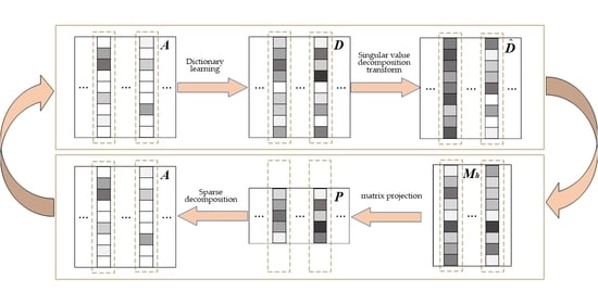
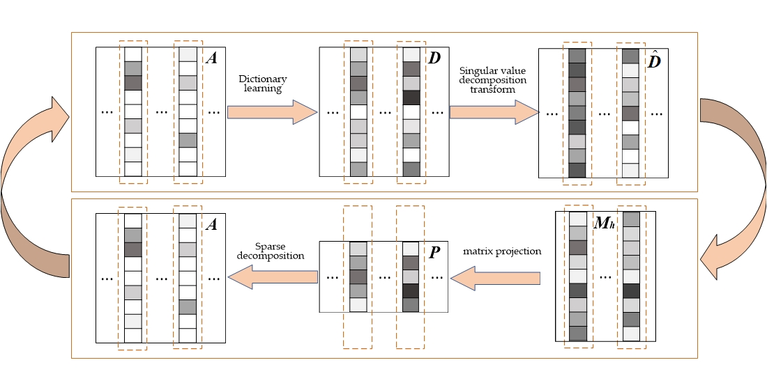
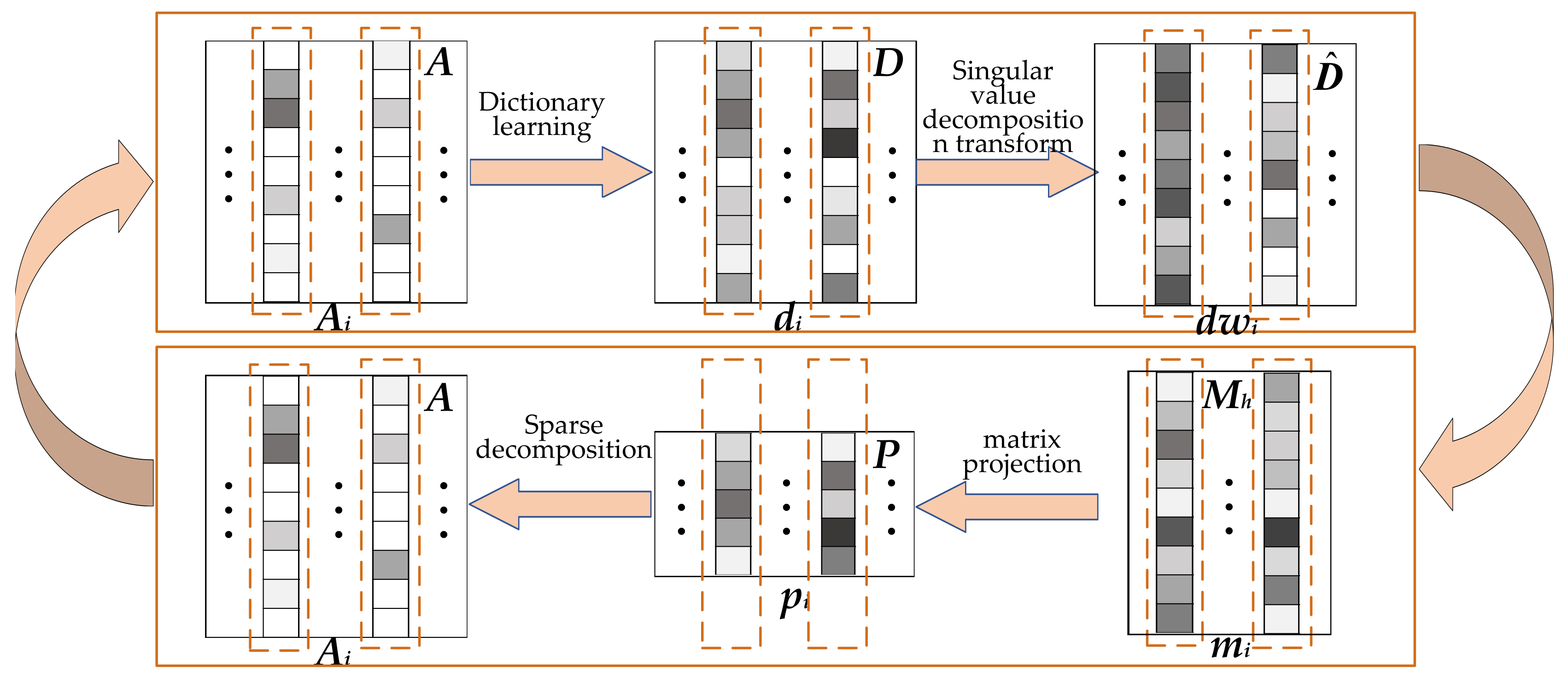
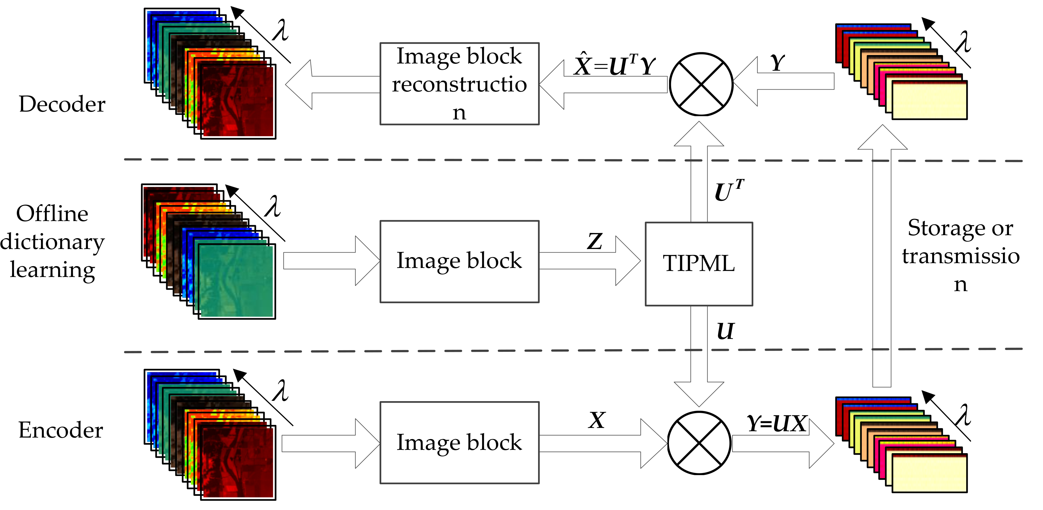
2.3. Task-Driven Invertible Projection Matrix Learning

In order to obtain a reversible projection transformation, we have to use prior knowledge to solve the invertible projection matrix. However, as we all know, it is very difficult to solve the low-dimensional invertible projection matrix U directly. Fortunately, it has been proven in Section 2.1 that the low-dimensional invertible projection matrix U can be solved indirectly by solving model (7). Model (7) is the problem of extracting principal components from dictionary D. Based on the theory in Section 2.2, a task-driven invertible projection matrix learning algorithm (TIPML) is proposed. In this algorithm, dictionary learning and singular value ʘ transformation are used as the core of the algorithm, and a dual-loop iterative training mechanism is established based on the core.
As shown in Figure 2, in order to ensure that more principal components of high-dimensional dictionary D are retained in the low-dimensional dictionary P. In TIPML, the singular value ʘ transformation is first used to make the energy of the dictionary D more concentrated. Next, the sparse representation coefficient A of the training data under the low-dimensional dictionary P is used to train the high-dimensional dictionary D. In this step, the low-dimensional dictionary P is used to train the high-dimensional dictionary D, which further increases the coupling between the two dictionaries and lets the principal components of the high-dimensional dictionary D be more retained in the low-dimensional dictionary P.
The specific implementation steps of the TIPML algorithm are shown in Algorithm 1.
Algorithm 1: TIPML
Input: Training data set X, number of iterations T, the singular value ʘ transformation parameter t,r, low-dimensional dictionary P dimension h, Signal sparsity K, and dimension of the data column N.
Output: Projection matrix U.
1: Initialization: Split the data set X into data columns xi (N × 1), I = 1,2,…, i is the index of the data column xi. Assuming X = [x1, x2,…, xn] (xiRN). The initial dictionary D is set as a DCT dictionary, D = [d1, d2,…,dn], (diRN).
2: Repeat
3:  Do singular value ʘ transformation to dictionary D: D = D Θ (t,r).
4:  Singular value decomposition: D = MΛVT.
5:  Calculate low-dimensional dictionary: P = MhTD.
6:  Based on the low-dimensional dictionary P, the OMP algorithm is used to sparse the data set X to obtain the sparse coefficient A = [a1, a2,…,an], update the index j = 1 of the dictionary atom.
7:  Repeat
8:   The error is calculated: E j = X l j d l a l T .
9:   The error is decomposed by SVD (rank-1 decomposition) into: E j u λ v T .
10:   Update dictionary: dj= u, Update sparsity coefficient: aj= λv.
11:   j = j + 1
12:  Until j > n
13: Until i Λ h i Λ is big enough, or reach the maximum number of iterations T.
14: Calculate the projection matrix: U = MhT.

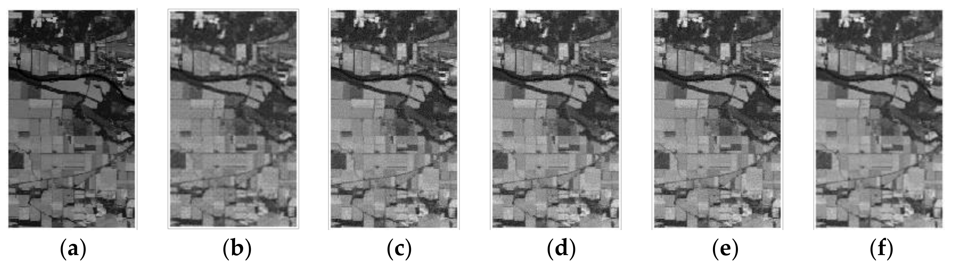
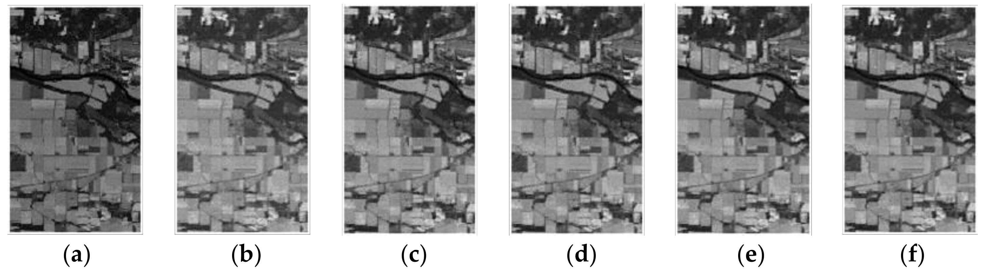
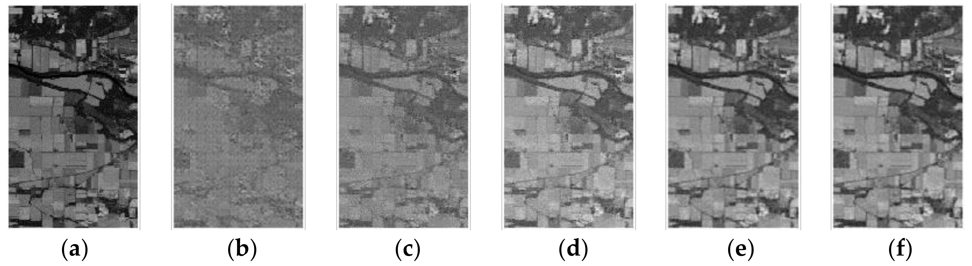
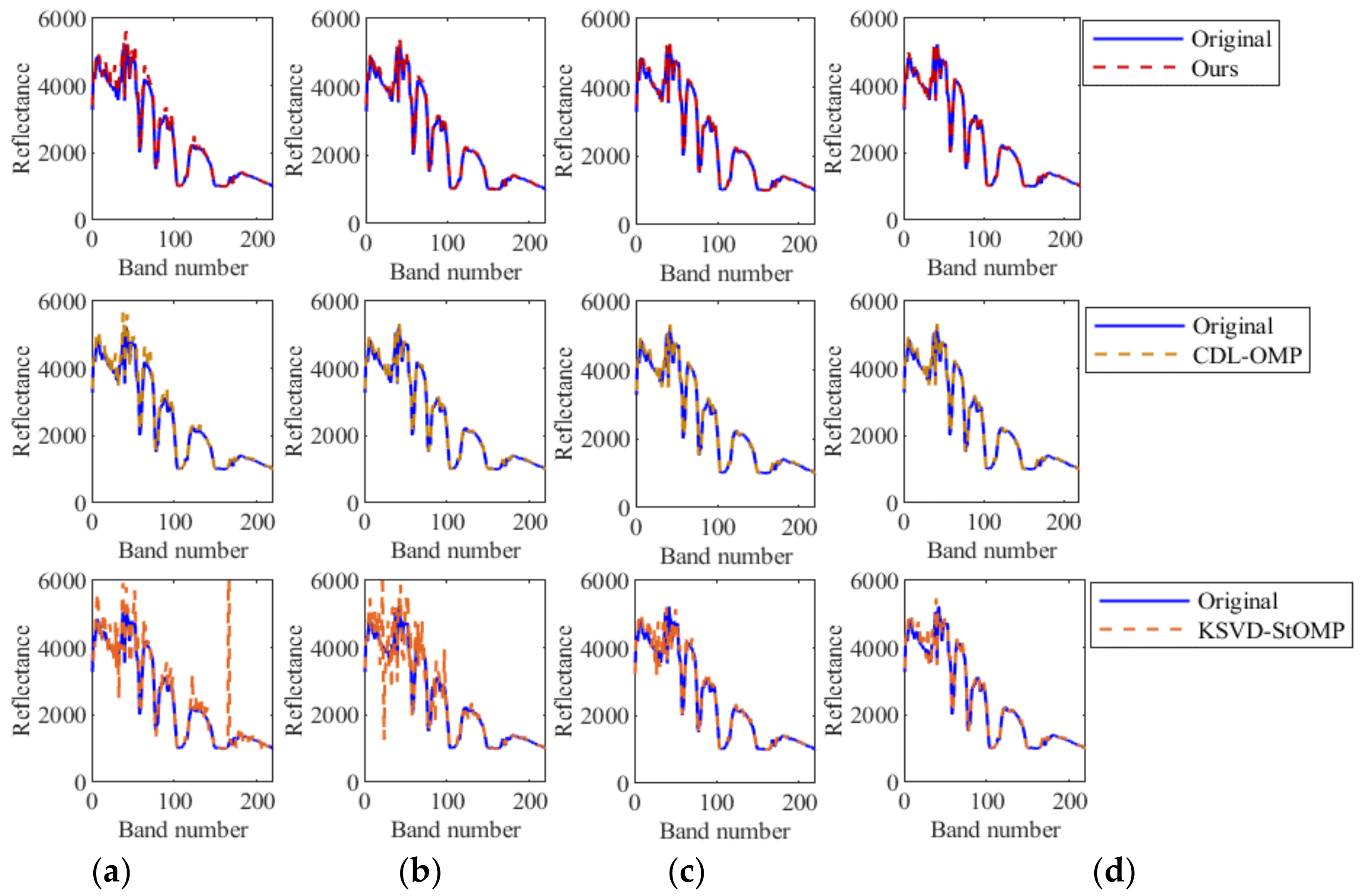
3. Simulation Experiment and Results

In order to verify the effectiveness of the algorithm proposed in this paper, the AVIRIS hyperspectral data image Indian Pine dataset [28] was selected as the experimental dataset. These hyperspectral data include 220 bands, and each pixel is stored in a 16-bit integer format. In the experiment, the most competitive sparse expression dictionary and reconstruction algorithm in compressed sensing were selected and compared with the algorithm proposed in this paper. Sparse expression dictionaries included DCT dictionary, KSVD dictionary, and CDL dictionary, and reconstruction algorithms included StOMP, OMP, GOMP, GROMP, CoSaMP, and SPL. Besides, the data compression algorithm PCA [29] has also been selected for comparison with the algorithm proposed in this paper. The average peak signal-to-noise ratio (PSNR), Spectral Angle Mapper (SAM), and reconstruction time T were selected as the evaluation indicators of the experiment, and the PSNR and reconstruction time T of the reconstructed image was obtained by setting different sampling rates (SR). The software and hardware environment of the test experiment are CPU: Intel(R) Core (TM) i7-9750H 2.6GHz, 8GB memory, and Windows 10 and MatLab 2019a.
The PSNR calculation formula is
P S N R = 10 l o g 10 M A X 2 1 m n i = 1 , j = 1 m , n x ( i , j ) x ( i , j ) 2
where x is the original image, is the reconstructed image, m and n respectively represent the length and width of the image, and MAX is the maximum value of image pixels.
The sampling rate calculation formula is
S R = M λ N λ
where Nλ is the dimension of the original data, and Mλ is the dimension of compressed sensing sampling.
The SAM calculation formula is
S A M = c o s 1 x T x ( x T x ) 1 2 ( x T x ) 1 2
where x is the original image, is the reconstructed image, xT and x’T are the transpose of matrix x and x’, respectively, and cos−1 is the arc cosine function.
As shown in Figure 3, the simulation experiment mainly included three stages, namely offline learning, data sampling (encoding), and data reconstruction (decoding). In the experiment, the data of the Indian Pine data set was divided into two parts: The training data set and the test data set. The transformation adjustment parameters of the TIPML algorithm were set to ‘t = 255′ and ‘r = 0.3′. In addition, the data set was processed in blocks with a block size of 16 × 16, and each small block was arranged into a column vector with a size of 256 × 1. First, the training set Z was used as the TIPML training sample to obtain the projection matrix U. Then, the projection matrix U was used as a reduced-dimensional sampling matrix of the test data X to obtain the observation data Y. Finally, the transposed UT of the projection matrix was used to back-project the low-dimensional sampling data Y to obtain the reconstructed data.
As shown in Figure 4, Figure 5 and Figure 6, the PSNR of the reconstructed image of the algorithm proposed in this paper, CDL-OMP algorithm, and KSVD-StOMP algorithm under different sampling rates (SR) are respectively given. By comparing the reconstructed images, it can be known that the KSVD-StOMP algorithm has the lowest image reconstruction accuracy at the same sampling rate. The reconstruction accuracy of the algorithm proposed in this paper is visually similar to that of the CDL-OMP algorithm. At low sampling rates (SR = 0.1), there is still a good reconstruction effect.
As shown in Figure 7, at different sampling rates, the original spectral line and the reconstructed spectral line at the (256, 1) pixel point, the experimental comparison methods are the algorithm proposed in this paper, CDL-OMP algorithm, and KSVD-StOMP algorithm. Comparing the experimental results, it can be seen that when the sampling rate SR = 0.2 in Figure 7b, the reconstructed spectrum line of the algorithm proposed in this paper almost coincides with the original spectrum line. When the sampling rate is low, the reconstructed spectrum of the proposed algorithm and the original spectrum have some errors, but the reconstruction effect is still slightly better than the CDL-OMP algorithm, and far better than the KSVD-StOMP algorithm. This is because when SR = 0.1 in Figure 7a, the dimension of the projection matrix Mλ = 26, which is much smaller than the original signal dimension Nλ = 256. When the original signal is projected into a low-dimensional space, too much information is lost, resulting in reduced reconstruction accuracy.
In order to further verify the superiority of the algorithm proposed in this paper, more compressed sensing algorithms and PCA algorithm were selected. As shown in Table 1, the PSNR under the same sampling rate in the table is the average of all PSNRs of 220-band images. The results in the comparison table show that the reconstructed image accuracy of the compressed sensing method based on the algorithm proposed in this paper is better than other algorithms, and it still has a higher reconstruction accuracy at low sampling rates.
As shown in Table 2, the SAM under the same sampling rate in the table is the average of all SAMs of 220-band images. For the convenience of comparison, the SAM data in the table is displayed in the form of scientific notation. The results in the comparison table show that the reconstructed image SAM still has a lower SAM at low sampling rates. In other words, the reconstructed spectrum is more similar to the original spectrum.
For compressed sensing algorithms, the running time T of the reconstruction algorithm is a very important evaluation index. As shown in Table 3, the running time T under the same sampling rate in the table is the mean value of the running time of 220-band image reconstruction, and the time unit recorded in the table is milliseconds. By comparing the experimental results, it can be seen that the running time T of the algorithm proposed in this paper is much lower than that of the traditional compressed sensing algorithm, and the running time is shortened by at least a hundred times. This is because the projection matrix U trained by the algorithm proposed in this paper is approximately invertible. In the reconstruction process, only the low-dimensional sampling matrix Y is left multiplied by UT. However, traditional compression sparse reconstruction algorithms require multiple matrix inversion and iterative operations. These operations are very time-consuming. Therefore, the real-time performance of the algorithm proposed in this paper is much higher than other algorithms. Besides, compared to data compression algorithm PCA, when we know the covariance matrix of the source in advance and find the eigenvalues, the time consumption of the TIPML algorithm is similar to that of the PCA algorithm. However, in practical applications, the covariance and eigenvalue of the source are unknown. We need to calculate the covariance and eigenvalue of the source, which will cause a lot of time to be consumed. Therefore, compared to traditional compressed sensing algorithms and traditional PCA data compression algorithms, the TIPML algorithm is more competitive.

4. Conclusions

HSI is the main tool for remote sensing and earth observation. The amount of valuable industrial and scientific data retrieved on the ground can be greatly increased by data compression technology. The resources of spaceborne equipment are very precious, and compression is placed on the sampling end by compressed sensing technology, which can save a lot of time and resources for hyperspectral imaging technology. Therefore, compressed sensing technology has huge application prospects in the field of hyperspectral compression. However, compressed sensing technology needs to solve underdetermined equations. In traditional algorithms, a lot of time and storage resources are spent in the sparse reconstruction process. Therefore, the high complexity of data reconstruction is also the biggest drawback of compressed sensing technology.
Aiming at the high computational complexity of compressed sensing technology and insufficient reconstruction accuracy, a task-driven invertible projection matrix learning algorithm was proposed by us. Our main contribution:
(1)
Derived the equivalent model of the invertible projection model theoretically, which converts the complex invertible projection training model into a coupled dictionary training model;
(2)
proposed a task-driven invertible projection matrix learning algorithm for invertible projection model training;
(3)
based on a task-driven reversible projection matrix learning algorithm, established a compressed sensing algorithm with strong real-time performance and high reconstruction accuracy.
Experimental verification has shown that the compressed sensing technology based on the algorithm proposed in this paper not only has higher reconstruction accuracy than traditional compressed sensing technology, but also has improved real-time performance by more than a hundred times. It is foreseeable that the algorithm proposed in this paper will have great application prospects in the field of hyperspectral image compression. In addition, the algorithm proposed in this paper can’t only be used in the fields of one-dimensional signal compression, two-dimensional image compression, and data denoising, but it will also have greater research value on hardware platforms such as FPGA and embedded devices due to its extremely low the complexity.

Author Contributions

Conceptualization, S.D.; methodology, S.D.; software, S.D.; validation, S.D.; formal analysis, S.D.; investigation, S.D.; resources, Z.W.; data curation, S.D.; writing—original draft preparation, S.D.; writing—review and editing, S.D.; visualization, S.D.; supervision, W.L and K.L.; project administration, W.L. and K.L.; funding acquisition, W.L. and K.L. All authors have read and agreed to the published version of the manuscript.

Funding

This research was funded by National Key Research and Development Program of China grant number 2018YFB2003304, National Natural Science Foundation of China grant number 61871218, Fundamental Research Funds for the Central Universities grant number NJ2019007 and NJ2020014, National Key Research and Development Program of China grant number 2017YFF0107304, 2017YFF0209700, 2016YFB1100205, and 2016YFF0103702.

Institutional Review Board Statement

Not applicable.

Informed Consent Statement

Not applicable.

Data Availability Statement

All data included in this study are available upon request by contact with the corresponding author.

Conflicts of Interest

The authors declare no conflict of interest.

References

  1. Parente, M.; Kerekes, J.; Heylen, R. A Special Issue on Hyperspectral Imaging [From the Guest Editors]. IEEE Geosci. Remote Sens. Mag. 2019, 7, 6–7. [Google Scholar] [CrossRef]
  2. Vohland, M.; Jung, A. Hyperspectral Imaging for Fine to Medium Scale Applications in Environmental Sciences. Remote Sens. 2020, 12, 2962. [Google Scholar] [CrossRef]
  3. Saari, H.; Aallos, V.-V.; Akujärvi, A.; Antila, T.; Holmlund, C.; Kantojärvi, U.; Mäkynen, J.; Ollila, J. Novel Miniaturized Hyperspectral Sensor for UAV and Space Applications. In Proceedings of the SPIE 7474, Sensors, Systems, and Next-Generation Satellites XIII, 74741M, SPIE Remote Sensing, Berlin, Germany, 31 August–3 September 2009. [Google Scholar] [CrossRef]
  4. Renhorn, I.G.E.; Axelsson, L. High spatial resolution hyperspectral camera based on exponentially variable filter. Opt. Eng. 2019, 58, 103106. [Google Scholar] [CrossRef]
  5. Pu, H.; Lin, L.; Sun, D.-W. Principles of Hyperspectral Microscope Imaging Techniques and Their Applications in Food Quality and Safety Detection: A Review. Compr. Rev. Food Sci. Food Saf. 2019, 18, 853–866. [Google Scholar] [CrossRef] [PubMed] [Green Version]
  6. Wang, L.; Lu, K.; Liu, P. Compressed Sensing of a Remote Sensing Image Based on the Priors of the Reference Image. IEEE Geosci. Remote Sens. Lett. 2015, 12, 736–740. [Google Scholar] [CrossRef]
  7. Donoho, D.L. Compressed sensing. IEEE Trans. Inf. Theory 2006, 52, 1289–1306. [Google Scholar] [CrossRef]
  8. Hsu, C.; Lin, C.; Kao, C.; Lin, Y. DCSN: Deep Compressed Sensing Network for Efficient Hyperspectral Data Transmission of Miniaturized Satellite. IEEE Trans. Geosci. Remote Sens. 2020. [Google Scholar] [CrossRef]
  9. Biondi, F. In Compressed Sensing Radar-New Concepts of Incoherent Continuous Wave Transmissions; IEEE: Piscataway, NJ, USA, 2015; pp. 204–208. [Google Scholar]
  10. Candes, E.J.; Romberg, J.; Tao, T. Robust uncertainty principles: Exact signal reconstruction from highly incomplete frequency information. IEEE Trans. Inf. Theory 2004, 52, 489–509. [Google Scholar] [CrossRef] [Green Version]
  11. Candes, E.J.; Tao, T. Near-Optimal Signal Recovery from Random Projections: Universal Encoding Strategies. Inf. Theory IEEE Trans. 2006, 52, 5406–5425. [Google Scholar] [CrossRef] [Green Version]
  12. Xue, H.; Sun, L.; Ou, G. Speech reconstruction based on compressed sensing theory using smoothed L0 algorithm. In Proceedings of the 2016 8th International Conference on Wireless Communications & Signal Processing (WCSP), Yangzhou, China, 13–15 October 2016; pp. 1–4. [Google Scholar] [CrossRef]
  13. Luo, H.; Zhang, N.; Wang, Y. Modified Smoothed Projected Landweber Algorithm for Adaptive Block Compressed Sensing Image Reconstruction. In Proceedings of the 2018 International Conference on Audio, Language and Image Processing (ICALIP), Shanghai, China, 16–17 July 2018; pp. 430–434. [Google Scholar] [CrossRef]
  14. Matin, A.; Dai, B.; Huang, Y.; Wang, X. Ultrafast Imaging with Optical Encoding and Compressive Sensing. J. Light. Technol. 2019, 761–768. [Google Scholar] [CrossRef]
  15. Dao, P.; Li, X.; Griffin, A. Quantitative Comparison of EEG Compressed Sensing using Gabor and K-SVD Dictionaries. In Proceedings of the 2018 IEEE 23rd International Conference on Digital Signal Processing (DSP), Shanghai, China, 19–21 November 2018; pp. 1–5. [Google Scholar] [CrossRef] [Green Version]
  16. Sana, F.; Katterbauer, K.; Al-Naffouri, T. Enhanced recovery of subsurface geological structures using compressed sensing and the Ensemble Kalman filter. In Proceedings of the 2015 IEEE International Geoscience and Remote Sensing Symposium (IGARSS), Milan, Italy, 26–31 July 2015; pp. 3107–3110. [Google Scholar] [CrossRef] [Green Version]
  17. Dehkordi, R.; Khosravi, H.; Ahmadyfard, A. Single image super-resolution based on sparse representation using dictionaries trained with input image patches. IET Image Process. 2020, 14, 1587–1593. [Google Scholar] [CrossRef]
  18. Silong, Z.; Yuanxiang, L.; Xian, W. Nonlinear dimensionality reduction method based on dictionary learning. Acta Autom. Sin. 2016, 42, 1065–1076. [Google Scholar]
  19. Vehkaperä, M.; Kabashima, Y.; Chatterjee, S. Analysis of Regularized LS Reconstruction and Random Matrix Ensembles in Compressed Sensing. IEEE Trans. Inf. Theory 2016, 62, 2100–2124. [Google Scholar] [CrossRef] [Green Version]
  20. Ziran, W.; Huachuang, W.; Jianlin, Z. Structural optimization of measurement matrix in image reconstruction based on compressed sensing. In Proceedings of the 2017 7th IEEE International Conference on Electronics Information and Emergency Communication (ICEIEC), Macau, China, 21–23 July 2017; pp. 223–227. [Google Scholar] [CrossRef]
  21. Zhang, W.; Tan, C.; Xu, Y. Electrical Resistance Tomography Image Reconstruction Based on Modified OMP Algorithm. IEEE Sens. J. 2019, 19, 5723–5731. [Google Scholar] [CrossRef]
  22. Qian, Y.; Zhu, D.; Yu, X. SAR high-resolution imaging from missing raw data using StOMP. J. Eng. 2019, 2019, 7347–7351. [Google Scholar] [CrossRef]
  23. Davenport, M.; Needell, D.; Wakin, M. Signal Space CoSaMP for Sparse Recovery with Redundant Dictionaries. IEEE Trans. Inf. Theory 2013, 59, 6820–6829. [Google Scholar] [CrossRef] [Green Version]
  24. Chen, S.; Feng, C.; Xu, X. Micro-motion feature extraction of narrow-band radar target based on ROMP. J. Eng. 2019, 2019, 7860–7863. [Google Scholar] [CrossRef]
  25. Trevisi, M.; Akbari, A.; Trocan, M. Compressive Imaging Using RIP-Compliant CMOS Imager Architecture and Landweber Reconstruction. IEEE Trans. Circuits Syst. Video Technol. 2020, 30, 387–399. [Google Scholar] [CrossRef] [Green Version]
  26. Wei, X. Reconstructible Nonlinear Dimensionality Reduction via Joint Dictionary Learning. IEEE Trans. Neural Netw. Learn. Syst. 2019, 30, 175–189. [Google Scholar] [CrossRef] [PubMed]
  27. Shufang, X. Theory and Method of Matrix Calculation; Peking University Press: Beijing, China, 1995; p. 7. [Google Scholar]
  28. Baumgardner, M.F.; Biehl, L.L.; Landgrebe, D.A. 220 Band AVIRIS Hyperspectral Image Data Set: 12 June 1992 Indian Pine Test Site 3. In Purdue University Research Repository; Purdue University: West Lafayette, IN, USA, 2015. [Google Scholar] [CrossRef]
  29. Lee, C.; Youn, S.; Jeong, T.; Lee, E.; Serra-Sagristà, J. Hybrid Compression of Hyperspectral Images Based on PCA with Pre-Encoding Discriminant Information. IEEE Geosci. Remote Sens. Lett. 2015, 12, 1491–1495. [Google Scholar] [CrossRef] [Green Version]
Figure 1. Block diagram of compressed sensing.
Remotesensing 13 00295 g001
Figure 2. Block diagram of TIPML (task-driven invertible projection matrix learning algorithm).
Remotesensing 13 00295 g002
Figure 3. Flow chart of simulation experiment.
Remotesensing 13 00295 g003
Figure 4. The original image and reconstructed image with band number 180, the compressed sensing algorithm is based on the TIPML algorithm, (a)The original images; (b) The sampling rate of the reconstructed image is SR = 0.1; (c) The sampling rate of the reconstructed image is SR = 0.2; (d) The sampling rate of the reconstructed image is SR = 0.3; (e) The sampling rate of the reconstructed image is SR = 0.4; (f) The sampling rate of the reconstructed image is SR = 0.5.
Remotesensing 13 00295 g004
Figure 5. The Original image and reconstructed image with band number 180, the compressed sensing algorithm is based on the CDL-OMP algorithm, (a) The original images; (b) The sampling rate of the reconstructed image is SR = 0.1; (c) The sampling rate of the reconstructed image is SR = 0.2; (d) The sampling rate of the reconstructed image is SR = 0.3; (e) The sampling rate of the reconstructed image is SR = 0.4; (f) The sampling rate of the reconstructed image is SR = 0.5.
Remotesensing 13 00295 g005
Figure 6. The Original image and reconstructed image with band number 180, the compressed sensing algorithm is based on KSVD-StOMP algorithm, (a) The original image; (b) The sampling rate of the reconstructed image is SR = 0.1; (c) The sampling rate of the reconstructed image is SR = 0.2; (d) The sampling rate of the reconstructed image is SR = 0.3; (e) The sampling rate of the reconstructed image is SR = 0.4; (f) The sampling rate of the reconstructed image is SR = 0.5.
Remotesensing 13 00295 g006
Figure 7. The original and reconstructed spectral lines of the pixel at coordinates (256, 1). From top to bottom, they are TIPML algorithm, CDL-OMP, and KSVD-StOMP. From the first column to the fourth column (a) The sampling rate SR = 0.1; (b) The sampling rate SR = 0.2;(c) The sampling rate SR = 0.3;(d) The sampling rate SR = 0.4.
Remotesensing 13 00295 g007
Table 1. The reconstructed average peak signal-to-noise ratio (PSNR) (dB) of hyperspectral images in all bands under different sampling rates.
MethodsSampling Rate
0.10.20.30.40.5
Ours61.2063.3964.1764.8665.63
PCA54.0956.1557.8459.4661.10
KSVD-StOMP51.0654.1059.2160.8761.51
KSVD-OMP31.3728.3026.9327.0827.20
KSVD-GOMP33.8530.3129.0228.6128.74
KSVD-GROMP34.3933.5933.5735.0435.72
KSVD-CoSaMP48.7049.6150.3050.1850.26
DCT-SPL38.2746.8354.1058.8160.70
DCT-StOMP30.4430.9731.5232.1732.96
CDL-StOMP60.6763.0663.3363.3363.33
CDL-OMP60.6763.0663.3363.3363.33
CDL-CoSaMP48.7949.9349.9449.9449.94
CDL-GROMP14.8322.9028.3933.2737.21
CDL-GOMP9.1913.7317.8521.6024.74
Table 2. The reconstructed average Spectral Angle Mapper (SAM) (Scientific notation) of hyperspectral images in all bands under different sampling rates.
MethodsSampling Rate
0.10.20.30.40.5
Ours1.17 × 10−81.16 × 10−81.18 × 10−81.18 × 10−81.14 × 10−8
PCA1.20 × 10−81.19 × 10−81.22 × 10−81.21 × 10−81.18 × 10−8
KSVD-StOMP8.39 × 10−41.16 × 10−81.19 × 10−81.18 × 10−81.15 × 10−8
KSVD-OMP1.45 × 10−16.06 × 10−35.03 × 10−41.18 × 10−81.32 × 10−3
KSVD-GOMP5.34 × 10−21.15 × 10−84.82 × 10−31.18 × 10−81.97 × 10−3
KSVD-GROMP1.22 × 10−31.16 × 10−83.19 × 10−21.17 × 10−81.07 × 10−2
KSVD-CoSaMP1.16 × 10−81.16 × 10−81.19 × 10−81.16 × 10−81.15 × 10−8
DCT-SPL1.14 × 10−81.18 × 10−81.15 × 10−81.17 × 10−81.15 × 10−8
CDL-StOMP1.17 × 10−81.16 × 10−81.19 × 10−81.17 × 10−81.15 × 10−8
CDL-OMP1.17 × 10−81.16 × 10−81.19 × 10−81.17 × 10−81.15 × 10−8
CDL-CoSaMP1.65 × 10−37.16 × 10−11.18 × 10−81.75 × 10−28.31 × 10−2
CDL-GROMP4.55 × 10−41.20 × 10−41.32 × 10−39.83 × 10−42.88 × 10−4
CDL-GOMP4.55 × 10−41.20 × 10−41.32 × 10−39.83 × 10−42.88 × 10−4
Table 3. The reconstructed average time (millisecond) of hyperspectral images in all bands under different sampling rates.
MethodsSampling Rate
0.10.20.30.40.5
Ours0.30.30.40.40.4
PCA0.30.40.40.40.4
KSVD-StOMP210.8443.7667.1934.61235.0
KSVD-OMP264.9401.8545.3594.0613.5
KSVD-GOMP101.7170.4206.2246.8252.3
KSVD-GROMP84.6131.7181.0186.7189.3
KSVD-CoSaMP302.7527.7597.3829.7877.4
DCT-SPL354.8355.1354.8357.0359.1
DCT-StOMP199.4437.6732.21085.21517.4
CDL-StOMP228.2503.3763.01054.01384.2
CDL-OMP209.5462.7696.1955.61261.4
CDL-CoSaMP341.3553.0635.0895.7943.9
CDL-GROMP75.5111.8150.4153.0157.3
CDL-GOMP167.7253.3317.4365.8375.5
Publisher’s Note: MDPI stays neutral with regard to jurisdictional claims in published maps and institutional affiliations.

