Matching Large Baseline Oblique Stereo Images Using an End-to-End Convolutional Neural Network

1. Introduction

Large baseline oblique stereo images play a crucial role in achieving realistic three-dimensional (3D) reconstruction [1], topographic mapping [2] and object extraction [3], owing to the advantages of stable image geometry, extensive coverage as well as abundant textures across the images. However, practitioners significantly change the viewpoints by increasing the baseline and oblique angle between the cameras, which lead to significant geometric deformation, radiometric distortion and local surface discontinuity across acquired images. Therefore, the large baseline oblique image matching still remains an open problem for practical use in both photogrammetry [4] and computer vision [5].

In the past few decades, researchers have proposed numerous feature matching algorithms invariant to certain transformations [6,7,8,9], most of which were targeting wide baseline stereo images. The popular feature matching methods, including but not limited to, scale invariant feature transform (SIFT) algorithm [6] and its modifications [7,8,9], mainly focus on extracting scale invariant features by constructing Gaussian pyramids while discarding the effects of geometric distortions such as affine distortion [10]. For addressing this shortcoming researchers have published affine invariant feature detectors [11,12,13,14], such as Harris-affine and Hessian-affine [11]. These more advanced algorithms exploit the auto-correlation matrix to iteratively estimate affine invariant regions. However, as the feature matching is relatively independent of feature detection, it was inevitable that the conjugate centers of affine invariant regions have more or less accidental errors. To improve the precision of conjugate points, Yao et al. [15] proposed a multi-level coarse to fine matching strategy where the errors of coordinates are compensated by least square matching (LSM). This process removed numerous controversial matches which were not beneficial to high quality 3D scene reconstruction. In [16], Mikolajczyk et al. designed a comprehensive evaluation that showed the maximally stable extremal regions (MSERs) [12] surpassed other algorithms in case of viewpoint changes, and further revealed that the SIFT descriptor performed best in most cases [17]. Despite these attempts in the literature and approaches to introduce affine invariant feature matching algorithms, the feature matching problem still exists for large baseline oblique stereo images with complex perspective distortions. Use of any aforementioned approaches on these images result in many false positives and few true positives, even some optimal integration strategies are adopted [15].

Over the past several years, deep learning has been shown to be capable of feature expression and generalization [18], which may provide novel references resulted in being used for large baseline oblique stereo image matching [19,20,21,22]. The area of CNN based detection learning is an active area of research. In [18], authors presented the first fully general formulation for learning local covariant feature detectors via a Siamese neural network. Based on this work, authors of [19] proposed to improve the detected features by enforcing known discriminability of pre-defined features. This treatment, however, has limited potency of the algorithm to these pre-defined features. In order to solve this problem, Doiphode et al. [20] introduced a modified scheme by incorporating triple covariant constraints which can learn to extract robust features without the need to define pre-defined features. A more effective feature detection approach is to detect the location of feature points by using a handcrafted algorithm and learn the direction or affine transformation of feature points by using a CNN [21]. Despite the fact that the estimated affine transformation using this method surpasses many handcrafted methods, it is not precise enough, compared to the MSERs [12]. Detone et al. [22] presented a SuperPoint network for feature point detection based on a self-supervised framework of homographic adaption. The final system performed well for geometric stereo correspondence.

Recently, CNN based descriptor learning has attracted great attention. By designing a CNN using L2Net, Tian et al. [23] proposed an approach to learn compact descriptors in the Euclidean space. This approach has shown performance improvements against existing handcrafted descriptors. Inspired by SIFT matching criterion, Mishchuk et al. [24] introduced HardNet based on L2Net to extract better descriptors with the same dimensionality as the SIFT descriptors. The HardNet structure, which was characterized by a triplet margin loss, was shown to maximize the distance between the closest positive and closest negative patches, and thus generated distinctive set of descriptors. Mishkin et al. [25] presented the AffNet architecture to learn affine invariant regions for wide baseline images. The AffNet architecture is modified from HardNet by reducing the number of dimensions by one half and final layer of 128 dimensions in HardNet was replaced with 3 dimensions representing the affine transformation parameters. Wan et al. [26] proposed a pyramid patch descriptor (PPD) based on a pyramid convolutional neural triplet network. This deep descriptor improved the matching performance for image pairs with both illumination and viewpoint variations. In a pioneering work, Han et al. [27] introduced a Siamese network architecture for descriptor learning. Later, In order to consider the impact of negative samples on network training, Hoffer et al. [28] proposed a triplet network architecture to generate the deep learning descriptors. Following this work, both SOSNet [29] and LogPolarDesc [30] focused on improving sampling schemes and loss functions. However, there are only a few algorithms that enhance descriptor performance via network improvements. Moreover, some studies combine additional information, such as geometry or global context, such as GeoDesc [31] and ContextDesc [32].

End-to-end matching approaches using CNN integrate the detector and descriptor of standard pipelines into a monolithic network, such as the LIFT method [33] that treats image matching as an end-to-end learning problem. To solve the multiple-view geometry problem, a self-supervised framework with homographic adaptation was used in [22] for training interest point detectors and descriptors. The more representative end-to-end matching networks, such as LFNet [34] and R2D2 [35], achieved joint learning of detectors and descriptors to improve the stability and repeatability of feature points in various cases. The extensive tests provided in [36] revealed that, in spite of the improved performance of end-to-end image matching networks, they cannot surpass handcrafted algorithms and multistep solutions.

The aforementioned approaches have several shortcomings when attempting to automatically produce accurate matches between large baseline oblique stereo images:

• complex geometric and radiometric distortions inhibit these algorithms to extract sufficient invariant features with a good repetition rate, and thus it would increase the probability of outliers;
• Universally repetitive textures in images may result in numerous non-matching descriptors with very similar Euclidean distances, due to the fact that the minimized loss functions only consider the matching descriptor and the closest non-matching descriptor;
• Because of the fact that feature detection and matching are carried out independently, the feature points to be matched using above methods can only achieve pixel-level accuracy.

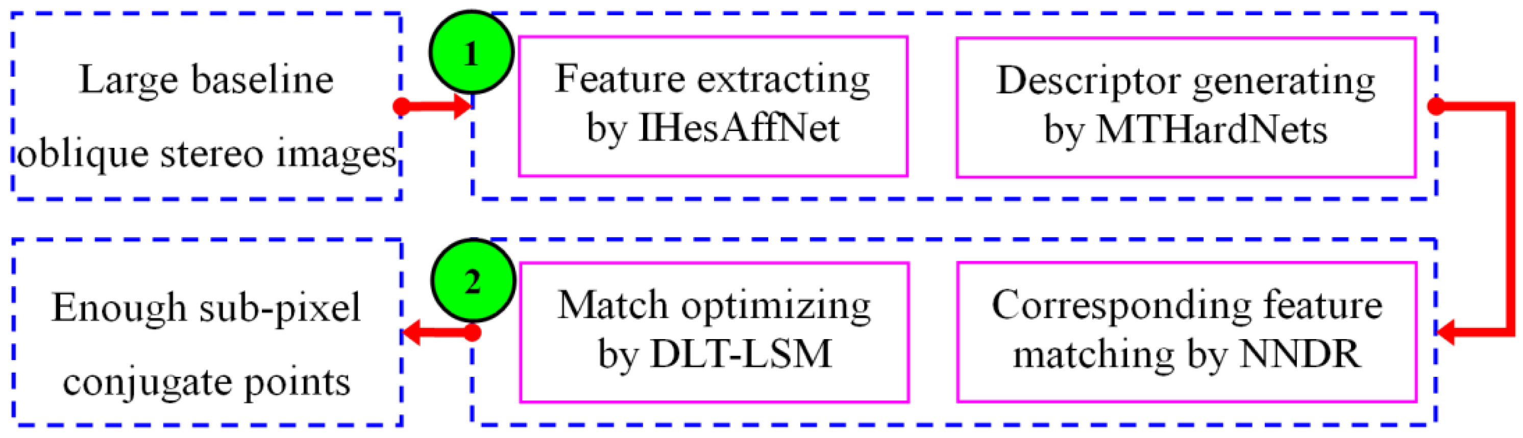
In order to address these problems, this article first generates affine invariant regions based on a modified version of the Hessian affine network (IHesAffNet). Following this step, we construct the MTHardNets and generate robust deep learning descriptors in 128 dimensions. Afterwards, identical regions are found using the nearest neighbor distance ratio (NNDR) metric. Furthermore, the positioning error of each match is effectively compensated by deep learning transform based least square matching (DLT-LSM), where the initial iterating parameters of DLT-LSM are provided based on the covariance matrix of deep learning regions. We conducted a comprehensive set of experiments on real large baseline oblique stereo image pairs to verify the effectiveness of our proposed end-to-end strategy, which outperforms the available state-of–the–art methods.

Our main contributions are summarized as follows. First, the improved IHesAffNet can obtain a sufficient number of affine regions with better repeatability and distribution. Second, the proposed MTHardNets can generate feasible descriptors with high discriminability. Third, the subpixel matching level can be achieved by DLT-LSM strategy for large baseline oblique images.

The remainder of this article is organized as follows. In Section 2, we present our approach in detail. In Section 3, we present the results. Discussion on the experimental results is given in Section 4. Section 5 concludes this article and presents future work.

2. Methodology

The purpose of this article is to automatically obtain a sufficient number of precise matches from large baseline oblique stereo images. Our proposed matching method is illustrated in Figure 1 and involves two main stages. In the first stage, the objective is to detect adequate affine invariant features with a uniform spatial distribution and generate distinctive descriptors. This stage is the basis and key for matching large baseline oblique images. In the second stage, the objective is to produce corresponding features and compensate for the position errors of the matches. This stage further verifies the matches achieved in first stage. We will detail the methodology in the following sections.

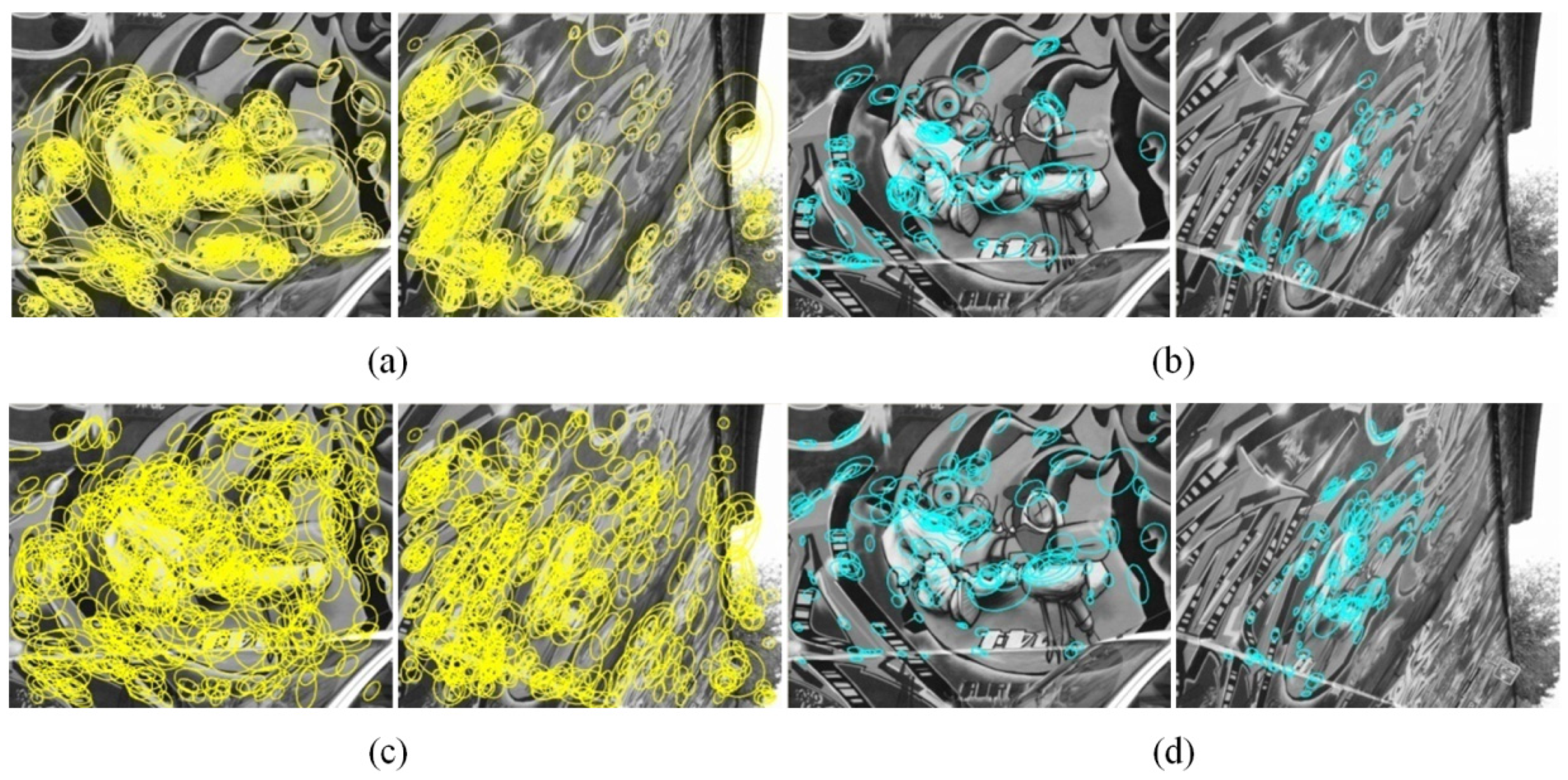
2.1. IHesAffNet for Feature Extraction

The quantity and quality of matches can be directly determined by feature detection. Many different deep learning structures for feature extraction were studied in [36] which concludes that it is difficult to select a learned detector network that can adapt to all images in all cases. However, the AffNet has shown to be more robust than other methods especially in wide baseline matching. Therefore, the AffNet is exploited to detect local invariant features in this article. There are seven convolutional layers in AffNet architecture, which was inherited from HardNet [24], but the number of dimensions in six former layers is reduced by one half and the final 128-D descriptor output layer is replaced by a 3-D output layer. For more details, please refer to [25].

Based on our tests, we verified that the original AffNet can cope with viewpoint and illumination variation across stereo images. Despite this, we also found that it invariably did not generate well-distributed and consistent results when both the baseline and oblique angle between the image pair are large. To overcome this problem, the optimization strategy, namely IHesAffNet, is proposed as follows.

First, a moderate number of Hessian features are respectively extracted from each image grid, and we only keep the Hessian points in each grid cell that satisfy the local information entropy threshold. More specifically, the average information entropy for arbitrary one grid cell is estimated by

$${{\rm Y}}_i=\frac{1}{a}{{\displaystyle \sum }}_{u=1}^a{\left(-{{\displaystyle \sum }}_{v=1}^b{\psi }_v{\log }_2{\psi }_v\right)}_u,$$

(1)

where a is the number of Hessian features in the grid cell, b is the number of different pixel value in feature region, and ${\psi }_v$ is the proportion of different pixel in feature region to the whole image pixels. Then, we set the threshold $T_i$ to be ${{\rm Y}}_i/2$ for each grid and adaptively remove the features with relatively low information entropy, thus we obtain local Hessians with global uniform distribution.

Second, we improve AffNet by constructing the optimal number of dimensions and obtain the affine invariant Hessian regions. Specifically, we search for best parameter set using multiple versions of AffNet with variations of dimensions (see

Table 1. Multiple versions of AffNet with different number of dimensions.

AffNet Version	Number of Dimensions in Each Layer
	1st Layer	2nd Layer	3rd Layer	4th Layer	5th Layer	6th Layer	7th Layer
AffNet1	32	32	64	64	128	128	3
AffNet2	28	28	56	56	112	112	3
AffNet3	24	24	48	48	96	96	3
AffNet4	20	20	40	40	80	80	3
AffNet5	16	16	32	32	64	64	3
AffNet6	12	12	24	24	48	48	3
AffNet7	8	8	16	16	32	32	3
AffNet8	4	4	8	8	16	16	3

) using the Graf1-6 stereo image dataset. The test results that represent these variations are plotted in Figure 2 which reveals that the AffNet5, namely the original AffNet, can reliably obtain a certain number of matches, but is slightly outperformed by AffNet6 in most epochs. Thus, in the remainder of the paper, we use AffNet6 as the improved version to extract affine invariant regions.

Third, the relatively stable region of each feature is selected by the following dual criteria: (i) the scale criterion is defined as $\left(W+H\right)/{\tau }_1\le \left(ϵ+\vartheta \right)/2\le \left(W+H\right)/{\tau }_2$, where $ϵ$ and $\vartheta$ respectively represent the major and minor axes of feature region, W and H are the width and height of image, respectively; (ii) the ratio criterion is defined as $ϵ/\vartheta \le e_{\mathrm{T}}$. Based on a large number of tests, the coefficients of scale criterion ${\tau }_1$ and ${\tau }_2$ are respectively set to be 160 and 20, and the ratio threshold $e_{\mathrm{T}}$ is set to be 6 in the article. The IHesAffNet for region extraction is concluded as Algorithm 1.

Algorithm 1. IHesAffNet Region Extraction.

Begin (1) Divide image into grids. (2) For one grid, extract Hessian points. Compute the average information entropy ${{\rm Y}}_i$ of the grid by Equation (1). (3) Set the threshold $T_i$ to be ${{\rm Y}}_i/2$, and remove all the Hessian points that lower than $T_i$. (4) Go to Step (2) and (3), until all the grids are processed. Then, save the Hessian points. (5) For one Hessian point, use AffNet6 to extract affine invariant region, until all the Hessian points are processed. Then, save the Hessian affine invariant regions. (6) Select the stable regions by dual criteria as $\left(W+H\right)/{\tau }_1\le \left(ϵ+\vartheta \right)/2\le \left(W+H\right)/{\tau }_2$ and $ϵ/\vartheta \le e_{\mathrm{T}}$. End

In order to verify the superiority of the IHesAffNet compared to the original AffNet, we have conducted comparison tests on numerous pairs of large baseline oblique stereo images. The first aim of this section is to improve the distribution quality of features in image space; and the second aim is to increase the repeatability score of the detection. Therefore, the first criterion is the distribution quality, which is detailed in [37,38], and can be calculated by

$$\{\begin{array}{ccc}\hfill \overline{E}& =& \frac{1}{m}{{\displaystyle \sum }}_{i=1}^m{E}_i\hfill \\ \hfill Z_i& =& 3\max \left({\theta }_i\right)/\pi \hfill \\ \hfill MDQ& =& \sqrt{{{\displaystyle \sum }}_{i=1}^m\left[\left(E_i/\overline{E}\right)-1\right]/\left(m-1\right)}\times \sqrt{{{\displaystyle \sum }}_{i=1}^m\left(Z_i-1\right)/\left(m-1\right)}\hfill \end{array},$$

(2)

where m denotes the total number of Delaunay triangles that are generated based on feature points and recursive strategy, $E_i$ and $\max \left({\theta }_i\right)$ respectively represent the area and the maximum angle (radians) of ith triangle, and the lower MDQ value indicates the better distribution of features. Normally, more matching features indicate higher repeatability score, thus we use the number of matched features as the second criterion. For a fair assessment, both AffNet and IHesAffNet employ SIFT descriptor and NNDR metric to generate matched features. Due to the limited space, we merely present the comparison results on Graf1-6 dataset in Figure 3 and

Table 2. Comparison of the AffNet and IHesAffNet in terms of feature distribution and repeatability on the Graf1-6 stereo image dataset.

Method	Left MDQ	Right MDQ	Matched Features
The HesAffNet	1.19	1.32	93
Our IHesAffNet	0.84	0.89	136

. The results show that our IHesAffNet can produce more well-distributed features and higher repeatability than the original AffNet.

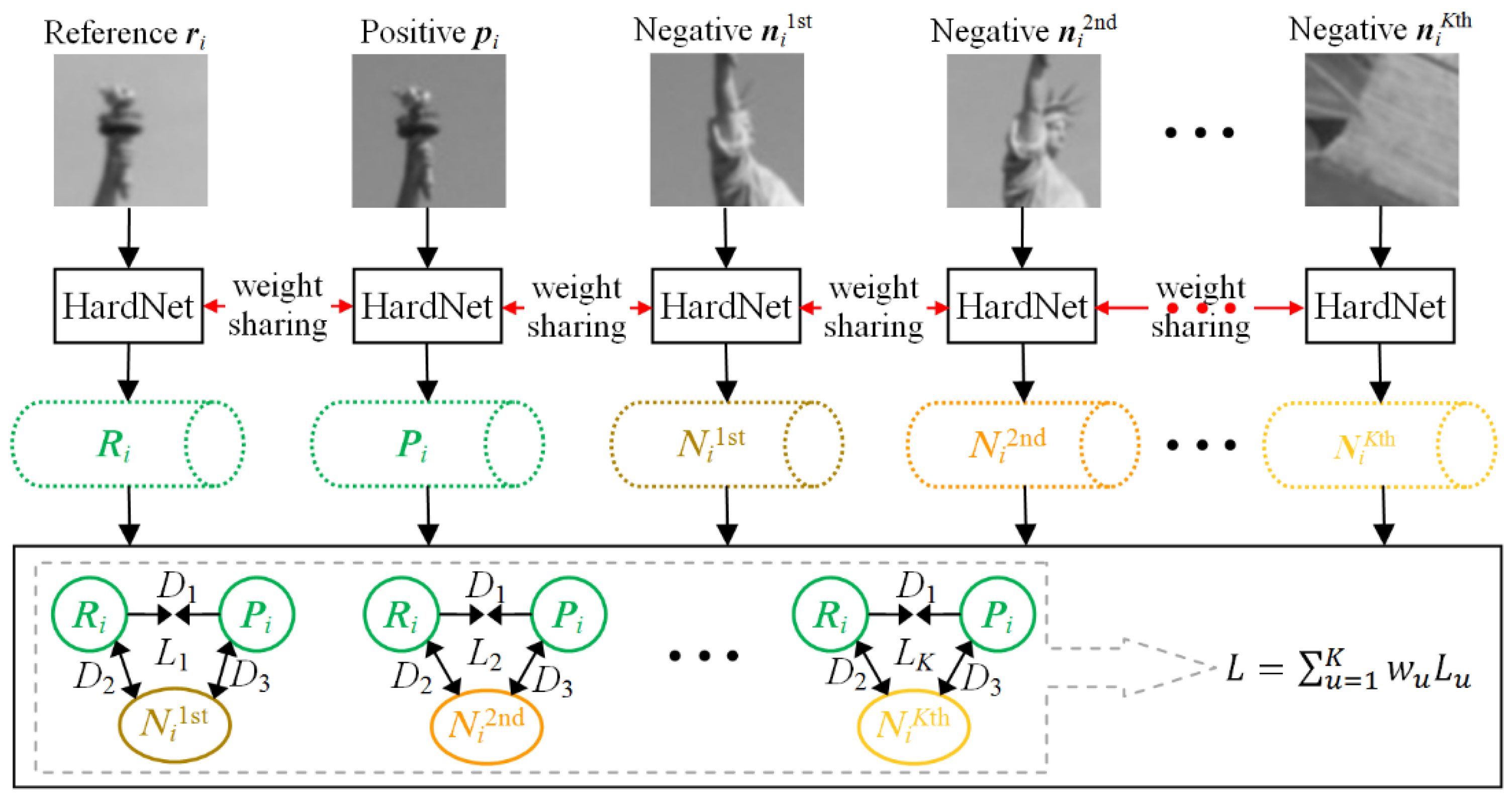
2.2. Descriptor Generating by MTHardNets

In addition to the feature detection discussed above, the descriptor extraction is another key factor for obtaining a sufficiently large number of correct matches from stereo images. The experiments demonstrated in [24] have shown that the HardNet possesses the most reasonable network architecture and outperforms existing deep learning-based descriptors. However, the sampling strategy adopted in HardNet only pulls the descriptor of one negative patch away from the reference or positive patches in the feature space, and it thus results in descriptors of negative patches with very close distances when there are extensive repetitive textures across stereo images. Therefore, to effectively avoid matching ambiguities, we design a schematic of multiple hard networks (MTHardNets) with K nearest negative samples using the empirical weighted loss function (EWLF), which is illustrated in Figure 4.

In the proposed network architecture, a batch of matching local patches $\mathit{\tau }={\left({\mathit{r}}_i,{\mathit{p}}_i\right)}_{i=1\dots m}$ is generated, where m is the number of samples in the batch, ${\mathit{r}}_i$ and ${\mathit{p}}_i$ stand for the reference and positive patches, respectively. A sequence of closest non-matching patches $\left({\mathit{n}}_i^{1\mathrm{st}},{\mathit{n}}_i^{2\mathrm{nd}},{\mathit{n}}_i^{K\mathrm{th}}\right)$ is selected for the current matching pair of $\left({\mathit{r}}_i,{\mathit{p}}_i\right)$, where the superscripts for $\mathit{n}$ 1st, 2nd and Kth respectively represent the first, second and Kth closest distances from $\left({\mathit{r}}_i,{\mathit{p}}_i\right)$. The current (K + 2) image patches are passed through HardNet and transformed into unit descriptors with 128-D. Moreover, the distance D₁ between matching descriptors R_i and P_i can be calculated by

$$D{\mathit{R}}_i,{\mathit{P}}_i=\sqrt{2-2{\mathit{R}}_i{\mathit{P}}_i},$$

(3)

Similarly, distances D₂ and D₃ between non-matching descriptors can also be computed. The purpose of the multiple networks is to push the distance D₁ as close as possible and simultaneously pull the distances D₂ and D₃ as far as possible to emphasize in class similarity and across class discrimination.

The proposed K nearest negative sampling strategy with EWLF proceeds by first estimating a distance matrix D from m pairs of corresponding descriptors $({\mathit{R}}_i, {\mathit{P}}_i)$ based on HardNet by using Equation (3):

$$\mathit{D}=\left[\begin{array}{ccccc}D\left({\mathit{R}}_1,{\mathit{P}}_1\right)& \cdots & D\left({\mathit{R}}_1,{\mathit{P}}_i\right)& \cdots & D\left({\mathit{R}}_1,{\mathit{P}}_m\right)\\ ⋮& \ddots & ⋮& ⋮& ⋮\\ D\left({\mathit{R}}_i,{\mathit{P}}_1\right)& \cdots & D\left({\mathit{R}}_i,{\mathit{P}}_i\right)& \cdots & D\left({\mathit{R}}_i,{\mathit{P}}_m\right)\\ ⋮& ⋮& ⋮& \ddots & ⋮\\ D\left({\mathit{R}}_m,{\mathit{P}}_1\right)& \cdots & D\left({\mathit{R}}_m,{\mathit{P}}_i\right)& \cdots & D\left({\mathit{R}}_m,{\mathit{P}}_m\right)\end{array}\right]=\left[\begin{array}{c}{\mathit{D}}_{R1P}\\ ⋮\\ {\mathit{D}}_{RiP}\\ ⋮\\ {\mathit{D}}_{RmP}\end{array}\right]={\left[\begin{array}{c}{\mathit{D}}_{RP1}\\ ⋮\\ {\mathit{D}}_{RPi}\\ ⋮\\ {\mathit{D}}_{RPm}\end{array}\right]}^{\mathrm{T}}.$$

(4)

This matrix provides the structure to select the K nearest negative descriptors. For one pair of corresponding descriptors $({\mathit{R}}_i, {\mathit{P}}_i)$, the respective distance arrays ${\mathit{D}}_{RiP}$ and ${\mathit{D}}_{RPi}$ are computed. The computed distances provide the K nearest negative descriptors $\left({\mathit{N}}_i^{1\mathrm{st}},\cdots ,{\mathit{N}}_i^{K\mathrm{th}}\right)$ according to values of $\left({\mathit{D}}_{RiP},{\mathit{D}}_{RPi}^{\mathrm{T}}\right)$. The selection is achieved by considering all K nearest negative descriptors and generate $\mathit{S}$ as:

$$\mathit{S}=\left[\begin{array}{c}\left({\mathit{R}}_1,{\mathit{P}}_1,\left({\mathit{N}}_1^{1\mathrm{st}},\cdots ,{\mathit{N}}_1^{K\mathrm{th}}\right)\right)\\ ⋮\\ \left({\mathit{R}}_i,{\mathit{P}}_i,\left({\mathit{N}}_i^{1\mathrm{st}},\cdots ,{\mathit{N}}_i^{K\mathrm{th}}\right)\right)\\ ⋮\\ \left({\mathit{R}}_m,{\mathit{P}}_m,\left({\mathit{N}}_m^{1\mathrm{st}},\cdots ,{\mathit{N}}_m^{K\mathrm{th}}\right)\right)\end{array}\right].$$

(5)

Based on K nearest negative descriptors, the empirical weighted loss function (EWLF) is generated using:

$$\{\begin{array}{c}{L}_1=\frac{1}{m}{{\displaystyle \sum }}_{i=1}^m\max \left(0,1+D\left({\mathit{R}}_i,{\mathit{P}}_i\right)-D\left(\left({\mathit{R}}_i,{\mathit{P}}_i\right),{\mathit{N}}_i^{1\mathrm{st}}\right)\right)\\ ⋮\\ L_K=\frac{1}{m}{{\displaystyle \sum }}_{i=1}^m\max \left(0,1+D\left({\mathit{R}}_i,{\mathit{P}}_i\right)-D\left(\left({\mathit{R}}_i,{\mathit{P}}_i\right),{\mathit{N}}_i^{K\mathrm{th}}\right)\right)\end{array},$$

(6)

where $D\left(\left({\mathit{R}}_i,{\mathit{P}}_i\right),{\mathit{N}}_i^{K\mathrm{th}}\right)$ is the distance between the non-matching and matching descriptors and can be computed by $D\left(\left({\mathit{R}}_i,{\mathit{P}}_i\right),{\mathit{N}}_i^{K\mathrm{th}}\right)=\min \left(\left({\mathit{R}}_i,{\mathit{N}}_i^{K\mathrm{th}}\right),\left({\mathit{P}}_i,{\mathit{N}}_i^{K\mathrm{th}}\right)\right)$. Finally, the EWLF model is established as:

$$L={{\displaystyle \sum }}_{u=1}^K{w}_u{L}_u,$$

(7)

where $w_u$ represents the empirical weight, and ${{\displaystyle \sum }}_{u=1}^K{w}_u=1$.

The key task of EWLF model is to enhance the discrimination of deep learning descriptors among repetitive patterns. In the following, we will empirically determine acceptable parameters for EWLF model based on the extensive tests. Both theory and experiments demonstrate that an increase in K improves discriminability of the descriptor for a large batch size. However, considering the limited GPU memory, we set K to 3 for EWLF calculations which simplifies the weight group set as $\mathit{W}=\left\{\left(w_1,w_2,w_3\right)|w_1\ge 0.50,w_1>w_2>w_3>0,w_1+w_2+w_3=1\right\}$.

Applying spatially uniform sampling, we obtain 564 groups of $\left(w_1,w_2,w_3\right)$ and the descriptor discrimination of each weight group can be computed using:

$$MDD=\frac{1}{m}{{\displaystyle \sum }}_{i=1}^m\overline{d}\left(\left({\mathit{R}}_i,{\mathit{P}}_i\right),{\mathit{N}}_i^{1\mathrm{st}},{\mathit{N}}_i^{2\mathrm{nd}},{\mathit{N}}_i^{3\mathrm{rd}}\right),$$

(8)

where $\overline{d}\left(\left({\mathit{R}}_i,{\mathit{P}}_i\right),{\mathit{N}}_i^{1\mathrm{st}},{\mathit{N}}_i^{2\mathrm{nd}},{\mathit{N}}_i^{3\mathrm{rd}}\right)$ represents the average distance of matching and non-matching descriptors. MDD is the metric of descriptor discrimination, such that the higher MDD value, the better the discrimination of the descriptor is. For each weight group, we train the MTHardNets based on the EWLF and compute the MDD. The statistical and comparative result for total weight groups is presented in Figure 5.

According to Figure 5, the serial number 366 of $\left(0.68, 0.22, 0.10\right)$ would achieve the highest MDD. Therefore, the Equation (7) can be specifically written as

$$L=0.68L_1+0.22L_2+0.10L_3.$$

(9)

In this article, the EWLF is obtained based on extensive tests, which is also the reason we refer to it as the empirical weighted loss function (EWLF). The pseudo-code of the MTHardNets descriptor is outlined in Algorithm 2.

Algorithm 2. MTHardNets Descriptor.

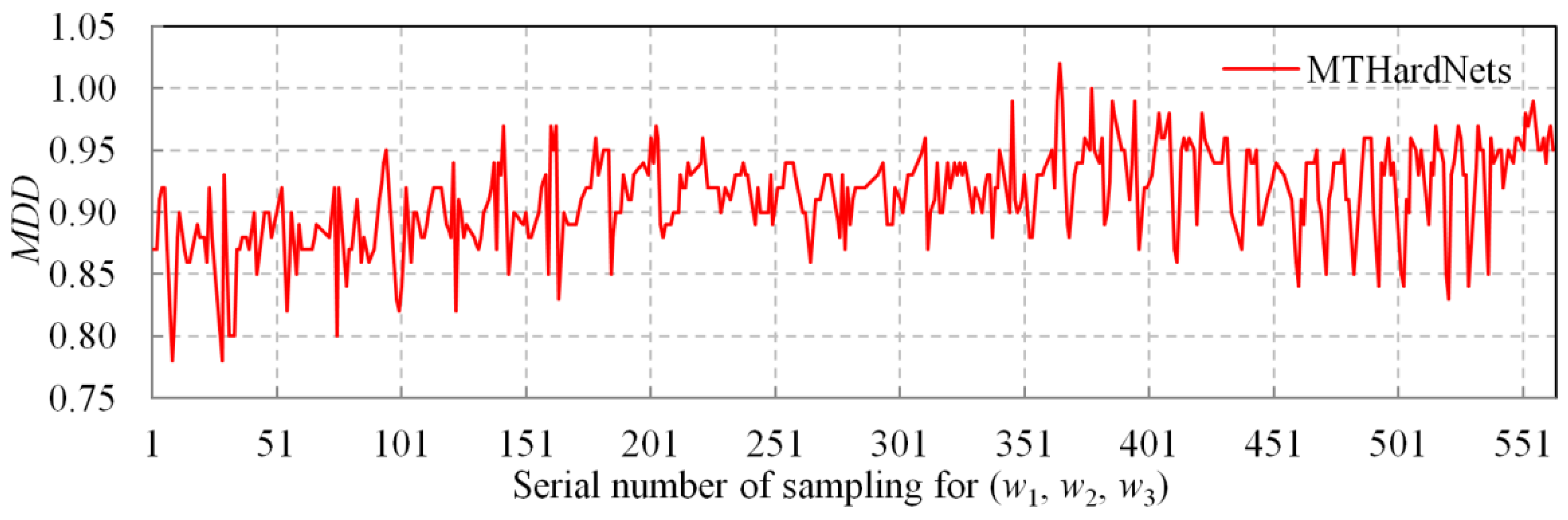
Begin (1) Given $\mathit{\tau }=\left({\mathit{r}}_i,{\mathit{p}}_i\right)$, then select $K$ closest non-matching patches $\left({\mathit{n}}_i^{1\mathrm{st}},{\mathit{n}}_i^{2\mathrm{nd}},{\mathit{n}}_i^{K\mathrm{th}}\right)$ for $\mathit{\tau }$. (2) Transform current $K+2$ patches into unit descriptors with 128-D, and compute distance D1 by Equation (3). Similarly, compute distances D2 and D3. (3) Estimate a distance matrix D by Equation (4), then generate $\mathit{S}$ by Equation (5). (4) Generate EWLF by using $S$ and Equation (6), and build EWLF model by Equation (7). (5) For each weight group, train the MTHardNets and compute MDD by Equation (8). (6) Use the highest MDD to simplify EWLF model as Equation (9). End

To further verify the superiority of our MTHardNets descriptor, we compare our approach with HardNet based on five pairs of matching points. The results of this experiment are shown in Figure 6 which reveals that proposed MTHardNets estimate smaller distance between the matching descriptors and larger distance between the non-matching descriptors. In other words, proposed MTHardNets descriptor has better discrimination when compared to HardNet.

In our pipeline, the IHesAffNet features are used as input to the MTHardNets which returns 128 dimensional descriptors. Following this step, the corresponding features are obtained using the NNDR metric and random sample consensus (RANSAC) is applied to remove outliers that does not satisfy underlying geometric relation between the images. Let $\mathit{\tau }=\left(\mathit{x},\mathit{A}\right)$ and ${\mathit{\tau }}^{\prime }=\left({\mathit{x}}^{\prime },{\mathit{A}}^{\prime }\right)$ represent an arbitrary pair of matching features, where $\mathit{x}$ and ${\mathit{x}}^{\prime }$ denote the centroids of two corresponding affine invariant regions $E\left(\mathit{x}\right)$ and $E^{\prime }\left({\mathit{x}}^{\prime }\right)$; $\mathit{A}$ and ${\mathit{A}}^{\prime }$ are the second moment affine matrices that can be learned by IHesAffNet, and the $\mathit{A}$ and ${\mathit{A}}^{\prime }$ respectively confirm $E\left(\mathit{x}\right)$ and $E^{\prime }\left({\mathit{x}}^{\prime }\right)$. Thus, the geometric transformation between $E\left(\mathit{x}\right)$ and $E^{\prime }\left({\mathit{x}}^{\prime }\right)$ can be expressed as:

$$E^{\prime }\left({\mathit{x}}^{\prime }\right)={\mathit{A}}^{\prime }{\mathit{A}}^{-1}E\left(\mathit{x}\right).$$

(10)

2.3. Match Optimizing by DLT-LSM

The feature points to be matched across images by using the above deep learning pipeline can only achieve pixel-level accuracy. The reason behind this is attributed to the fact that feature detection and matching are carried out independently. In order to mitigate this shortcoming, we employ a deep learning transform based least square matching (DLT-LSM) strategy. Let the neighborhood centered at a feature point $\mathit{x}$ contain $\left(2\lambda +1\right)\times \left(2\lambda +1\right)$ pixels, and suppose that the geometric deformation $H$ between the corresponding small neighborhoods of $x$ and $x^{\prime }$ can be well represented by:

$$\{\begin{array}{c}{u}^{\prime }=b_{1}u+b_{2}v+b_3\\ v^{\prime }=b_{4}u+b_{5}v+b_6\end{array},$$

(11)

Let $\mathit{H}=\left[\begin{array}{cc}\mathit{B}& \mathit{T}\end{array}\right]$, where $\mathit{B}=\left[\begin{array}{cc}{b}_1& b_2\\ b_4& b_5\end{array}\right]$ represents the affine deformation, $\mathit{T}=\left[\begin{array}{c}{b}_3\\ b_6\end{array}\right]$ is the translation deformation. If we write a pair of correlation windows $\mathit{\Omega }$ and ${\mathit{\Omega }}^{\prime }$, respectively centered at $\mathit{x}$ and ${\mathit{x}}^{\prime }$ as

$$\mathit{\Omega }=\mathit{I}\left(\mathit{x}+\mathit{u}\right), {\mathit{\Omega }}^{\prime }={\mathit{I}}^{\prime }\left({\mathit{x}}^{\prime }+\mathit{H}\mathit{u}\right),$$

(12)

where $\mathit{I}$ and ${\mathit{I}}^{\prime }$ are the intensity values respectively of the left and right images. Using these definitions, the correlation coefficient $\rho$ between $\mathit{\Omega }$ and ${\mathit{\Omega }}^{\prime }$ can be calculated by

$$\rho =\frac{{{\displaystyle \sum }}_{i=-\lambda }^{\lambda }{{\displaystyle \sum }}_{j=-\lambda }^{\lambda }\left({\mathit{\Omega }}_{ij}-\mu \left(\mathit{\Omega }\right)\right)\left({\mathit{\Omega }}_{ij}^{\prime }-\mu \left({\mathit{\Omega }}^{\prime }\right)\right)}{\sqrt{{{\displaystyle \sum }}_{i=-\lambda }^{\lambda }{{\displaystyle \sum }}_{j=-\lambda }^{\lambda }{\left({\mathit{\Omega }}_{ij}-\mu \left(\mathit{\Omega }\right)\right)}^2{{\displaystyle \sum }}_{i=-\lambda }^{\lambda }{{\displaystyle \sum }}_{j=-\lambda }^{\lambda }{\left({\mathit{\Omega }}_{ij}^{\prime }-\mu \left({\mathit{\Omega }}^{\prime }\right)\right)}^2}},$$

(13)

where $\mu \left(\mathit{\Omega }\right)$ and $\mu \left({\mathit{\Omega }}^{\prime }\right)$ are the mean pixel values of corresponding windows; the pixel value ${\mathit{\Omega }}_{ij}$ is directly obtained from the left image, and the pixel value ${\mathit{\Omega }}_{ij}^{\prime }$ is produced based on a local bilinear interpolation of right image, that is a good trade-off between efficiency and accuracy.

According to Equation (12) and introducing linear radiometric distortion parameters $h_0$ and $h_1$, we establish the affine transform model based LSM equation, which can be further linearized to be a LSM error equation as

$$V=\mathit{C}\mathit{X}-L,$$

(14)

where $\mathit{X}={\left[\begin{array}{ccccc}d{h}_0& d{h}_1& d{b}_1& \cdots & d{b}_6\end{array}\right]}^{\mathrm{T}}$, $\mathit{C}=\left[\begin{array}{cccccccc}1& g^{\prime }& g_u^{\prime }& u{g}_u^{\prime }& v{g}_u^{\prime }& g_v^{\prime }& u{g}_v^{\prime }& v{g}_v^{\prime }\end{array}\right]$, $L=h_0+h_1\mathit{\Omega }-{\mathit{\Omega }}^{\prime }$, $g^{\prime }$ is the pixel value of ${\mathit{x}}^{\prime }$, and $g_u^{\prime }$ and $g_v^{\prime }$ represent the gradients at horizontal and vertical directions, respectively. This LSM error equations are applied for all pixels within the neighborhoods of $\mathit{x}$ and ${\mathit{x}}^{\prime }$. By minimizing this cost, the error correction matrix $\mathit{X}$ that includes eight parameter correction values, can be iteratively estimated. Compared with the affine distortion, the radiometric distortion and translation deformation are small such that we may set their initial values to be: $h_0^0=0$, $h_1^0=1$ and $b_3^0=b_6^0=0$. Then, the initial parameters of affine deformation matrix $\mathit{B}$ can be set according to the deep learning transform (DLT) of Equation (10), namely $\mathit{B}={\mathit{A}}^{\prime }{\mathit{A}}^{-1}$. The algorithm of DLT-LSM is described as Algorithm 3.

Algorithm 3. DLT-LSM.

Begin (1) For one correspondence $\mathit{x}$ and ${\mathit{x}}^{\prime }$, determine the initial affine transform $\mathit{B}$ by Equation (10). Initialize $\mathit{H}$ using $\mathit{B}$. Set the threshold of maximum iterations to be $N_{\mathrm{T}}$. (2) Build correlation windows $\mathit{\Omega }$ and ${\mathit{\Omega }}^{\prime }$ by Equations (11) and (12), and then compute $\rho$ by Equation (13). (3) Build LSM error equation as Equation (14), then compute $\mathit{X}$ and update $\mathit{H}$. If the number of iterations $N$ is less than $N_{\mathrm{T}}$, then go to Step (2); otherwise, correct ${\mathit{x}}^{\prime }$ by Equation (15). End

Using this formulation, the matching regions around the feature points can be optimized by DLT-LSM, provided it is supplied with good initial values for distortion parameters. In this section, given one pair of corresponding features, the affine transform matrix $\mathit{H}$ is initialized by the DLT strategy and is then iteratively updated. Furthermore, the original matching point ${\mathit{x}}^{\prime }$ can be precisely compensated by

$${\widehat{\mathit{x}}}^{\prime }={\mathit{x}}^{\prime }+\mathit{H}\mathit{x}.$$

(15)

The parameter that specifies the neighborhood around $\mathit{x}$ to set to $\lambda =25$ pixels, and a maximum of ten iterations are used in our DLT-LSM optimization. We randomly selected two pairs of conjugate neighborhoods, whose affine parameters have been obtained by our deep learning method, are presented in

Table 3. Conjugate neighborhoods, affine transform error $\epsilon$ (pixels), and correlation coefficient $\rho$ are corrected by DLT-LSM iterations.

	Left Neighborhood	Initial Right Neighborhood	First Iteration	Second Iteration	Third Iteration	Fourth Iteration
Window border
		ε = 2.635	ε = 2.244	ε = 1.290	ε = 0.837	ε = 0.516
Correlation windows
		ρ = 0.569	ρ = 0.638	ρ = 0.805	ρ = 0.919	ρ = 0.957
Window border
		ε = 1.278	ε = 0.860	ε = 0.553	ε = 0.375	ε = 0.241
Correlation windows
		ρ = 0.832	ρ = 0.915	ρ = 0.949	ρ = 0.957	ρ = 0.965

. The table lists the affine transform error $\epsilon$ which is estimated based on the ground truth affine matrix ${\mathit{H}}_0$ and following Equation

$$\epsilon =\Vert {\widehat{\mathit{x}}}^{\prime }-{\mathit{H}}_0\mathit{x}\Vert .$$

(16)

Table 3 shows that the DLT-LSM iteration can converge very rapidly for two different image patches with significant geometric and radiometric deformations. It further indicates that our DLT strategy would provide good affine parameter values for DLT-LSM, and thus the corresponding feature points are optimized to be subpixel-level accuracy.

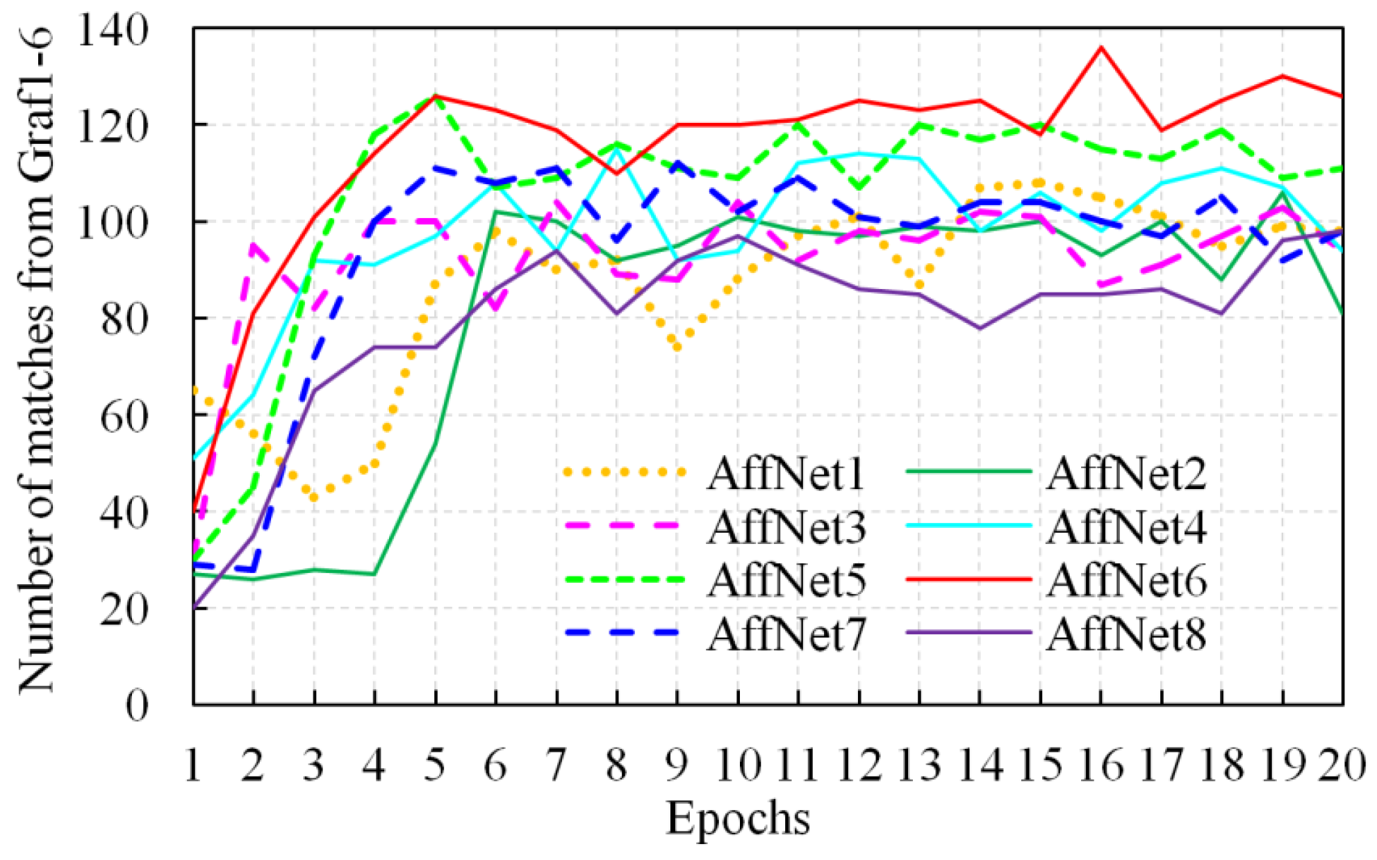
2.4. Training Dataset and Implementation Details

We used the open dataset, UBC Phototour [39] for training. It includes six subsets: Liberty, Liberty_harris, Notredame, Notredame_harris, Yosemite, Yosemite_harris, and there are 2 × 400 k normalized 64 × 64 patches in each dataset. All of the matching patches are verified by 3D reconstruction model. Both the IHesAffNet and the MTHardNets are trained with the models implemented using the Pytorch library [40]. In IHesAffNet training, there are 1024 triplet samples in a batch, and all image patches are resized to 32 × 32 pixels. Optimization is done by stochastic gradient descent strategy with learning rate 0.005, momentum 0.9, and weight decay 0.0001, and the model trained 20 epochs on RTX2080Ti GPU for every training data set. MTHardNets training is similar to IHesAffNet, but we use the proposed EWLF function to train the model with the learning rate of 10, and 1024 quintuple samples are prepared in a batch. Additionally, data augmentation is applied in both trainings to prevent over-fitting.

3. Results

3.1. Test Data and Evaluation Criteria

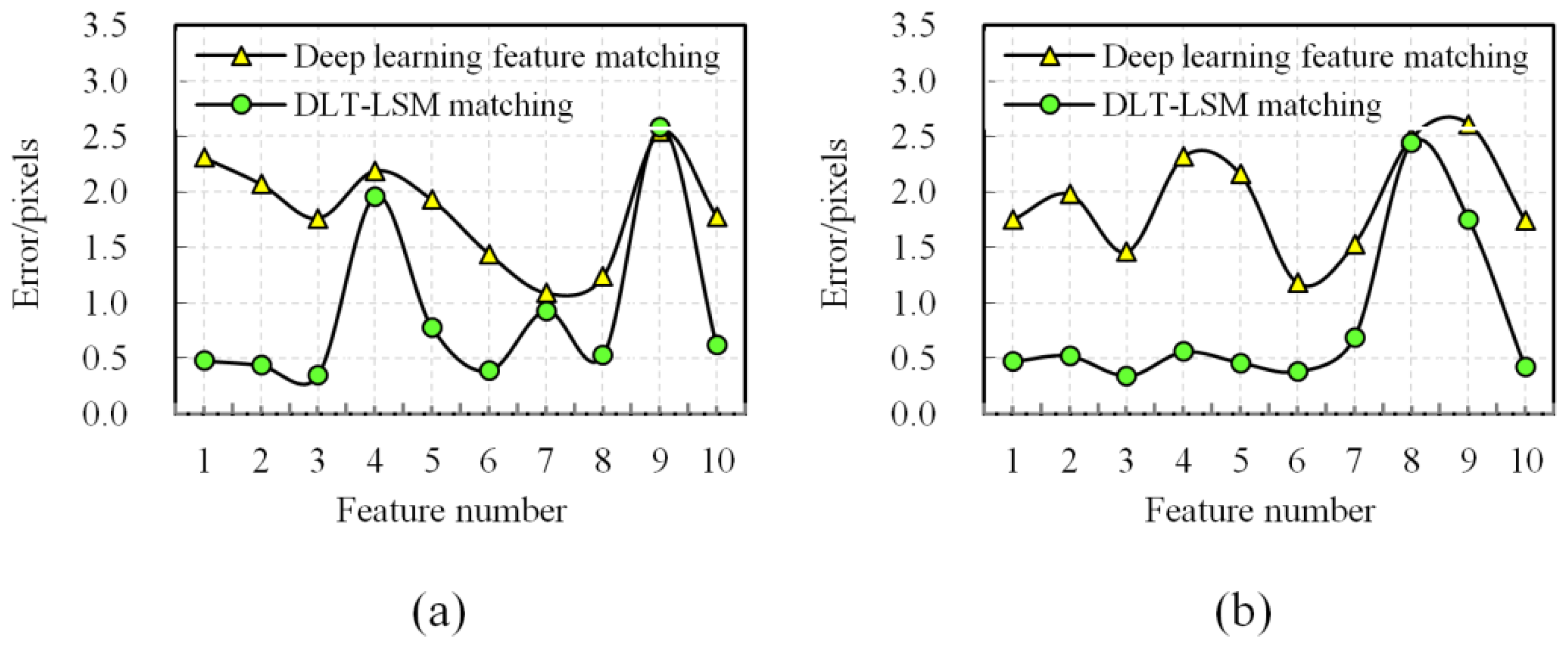
In order to test the performance of the proposed method, we selected six groups (A–F) of stereo images with large differences in viewpoints. The image pairs (A–C) are large baseline images acquired from the ground, and (D–F) were large baseline oblique images taken from an unmanned aerial vehicle (UAV). All groups of image data have severe geometric and radiometric distortions and cover various scenes with poor or repetitive textures. The image-to-image affine transform matrix ${\mathit{H}}_0$ was estimated by the strategy presented in [41] for each groups of stereo images and used as a ground truth. Additionally, five indexes were chosen to comprehensively estimate the effectiveness of method:

• Number of correct correspondences $n_{{\epsilon }_0}$ (the unit is pair): The matching error is calculated using ${\mathit{H}}_0$ and Equation (16). If the error of a corresponding point is less than the given threshold ${\epsilon }_0$ (1.5 pixels in our experiment), it was regarded as a inlier and used to compute $n_{{\epsilon }_0}$.
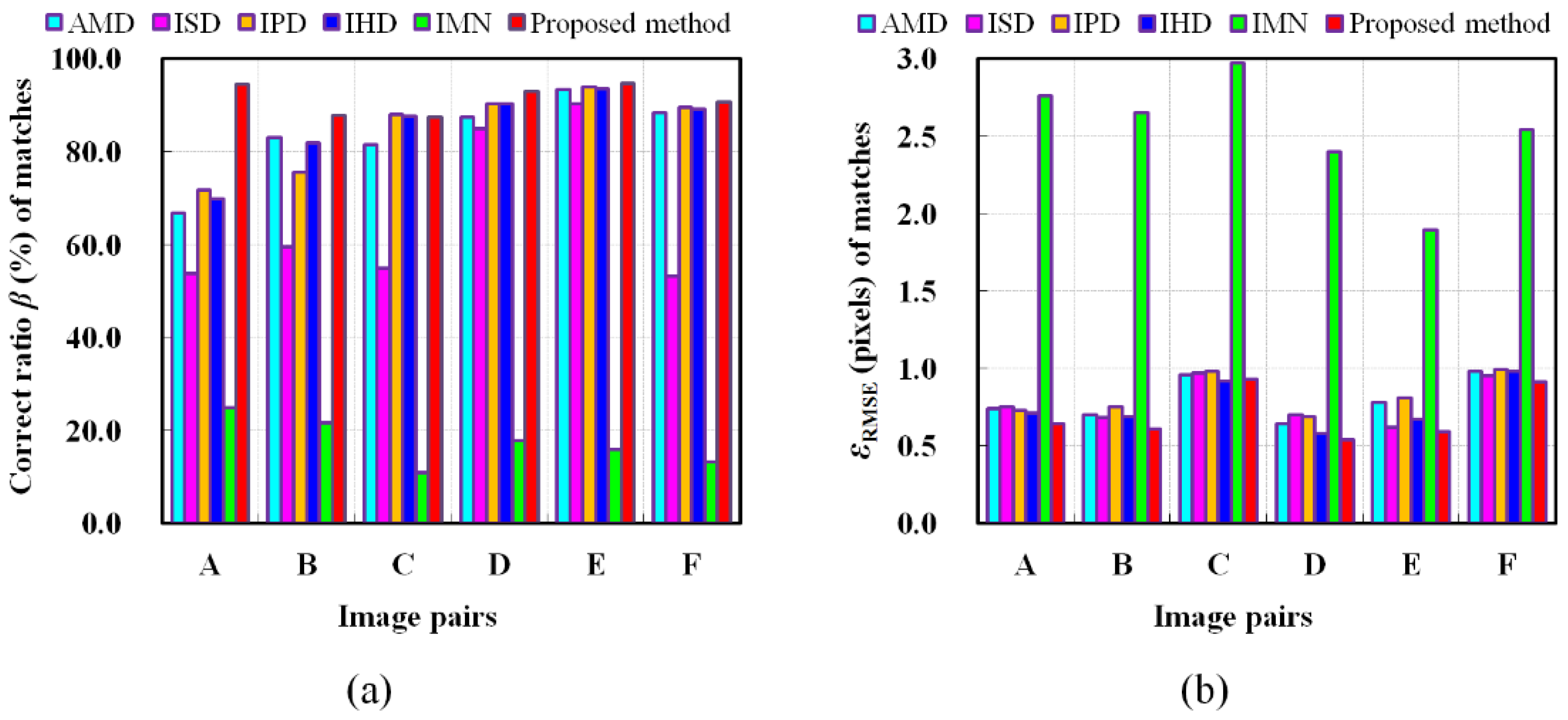
• Correct ratio β (in percentage, %) of matches: It is computed by $\beta =n_{{\epsilon }_0}/num$, where num (the unit is pair) is the number of total matches.
• Root mean square error ${\epsilon }_{\mathrm{RMSE}}$ (the unit is pixel) of matches: It is calculated by

  $${\epsilon }_{\mathrm{RMSE}}=\sqrt{\frac{1}{num}{{\displaystyle \sum }}_{i=1}^m{\mathit{y}}_i^{\prime }-{\mathit{H}}_0{\mathit{y}}_i{}^2},$$

  (17)
• Matching distribution quality MDQ: Lower MDQ value indicates the geometric homogeneity of the Delaunay triangles, which are generated based on matched points. Thus, the MDQ can be a uniform distribution metric of matches. This index is estimated by previous Equation (2).
• Matching efficiency η (the unit is second per pair of matching points): We compute the η according to average run time for one pair of corresponding points, namely $\eta =t/num$, where t (the unit is second) denotes the total test time of the algorithm.

3.2. Experimental Results of the Key Steps of the Proposed Method

Considering that the proposed approach includes three key steps, e.g., feature extraction, descriptor generation, and matching, we conduct comparison experiments based on six different matching algorithms to check the validity of each key step for six different methods: AMD, ISD, IPD, IHD, IMN, and the proposed method.

For intuitive understanding, we present each key step of six different methods in

Table 4. List of six different methods, namely, the AMD, the ISD, the IPD, the IHD, the IMN, and the proposed method.

Steps	AMD	ISD	IPD	IHD	IMN	Proposed Method
Feature extracting	AffNet [25]	IHesAffNet	IHesAffNet	IHesAffNet	IHesAffNet	IHesAffNet
Descriptor generating	MTHardNets	SIFT [6]	PPD [26]	HardNet [24]	MTHardNets	MTHardNets
Match optimizing	DLT-LSM	DLT-LSM	DLT-LSM	DLT-LSM	Null	DLT-LSM

, where “Null” denotes that the current step is not applicable. For a fair and objective evaluation, we exploit a unified strategy to reject inconsistent matches.

Table 5. Number of correct correspondences obtained by the AMD, ISD, IPD, IHD, IMN, and proposed method based on six groups of stereo images. Bold font denotes the best results.

Image Pair	AMD	ISD	IPD	IHD	IMN	Proposed Method
A	78	21	86	92	41	152
B	219	35	203	235	87	349
C	313	85	409	402	164	662
D	329	90	339	348	97	397
E	912	120	937	921	196	972
F	375	42	401	398	93	408

records the number of correct correspondences achieved by six different methods.

Table 6. The total test time (the unit is second) of the AMD, ISD, IPD, IHD, IMN, and proposed method based on six groups of stereo images. Bold font denotes the best results.

Image Pair	AMD	ISD	IPD	IHD	IMN	Proposed Method
A	29.02	24.09	29.36	30.45	29.14	31.49
B	32.79	27.49	33.45	34.58	33.20	36.55
C	39.60	36.52	43.10	42.70	39.05	45.73
D	40.14	35.60	42.08	41.83	40.57	44.61
E	47.05	41.65	48.74	49.06	43.74	52.32
F	40.33	35.94	40.16	41.63	40.92	43.80

denotes the total test time of six different methods. Comparative results of correct ratio (%) and root mean square error (pixels) of matches are displayed in Figure 7 to inspect the effectiveness and accuracy of these methods.

3.3. Experimental Results of Comparison Methods

We further verify the performance of the proposed method and contrast four methods on oblique image matching as follows. The four methods include the following:

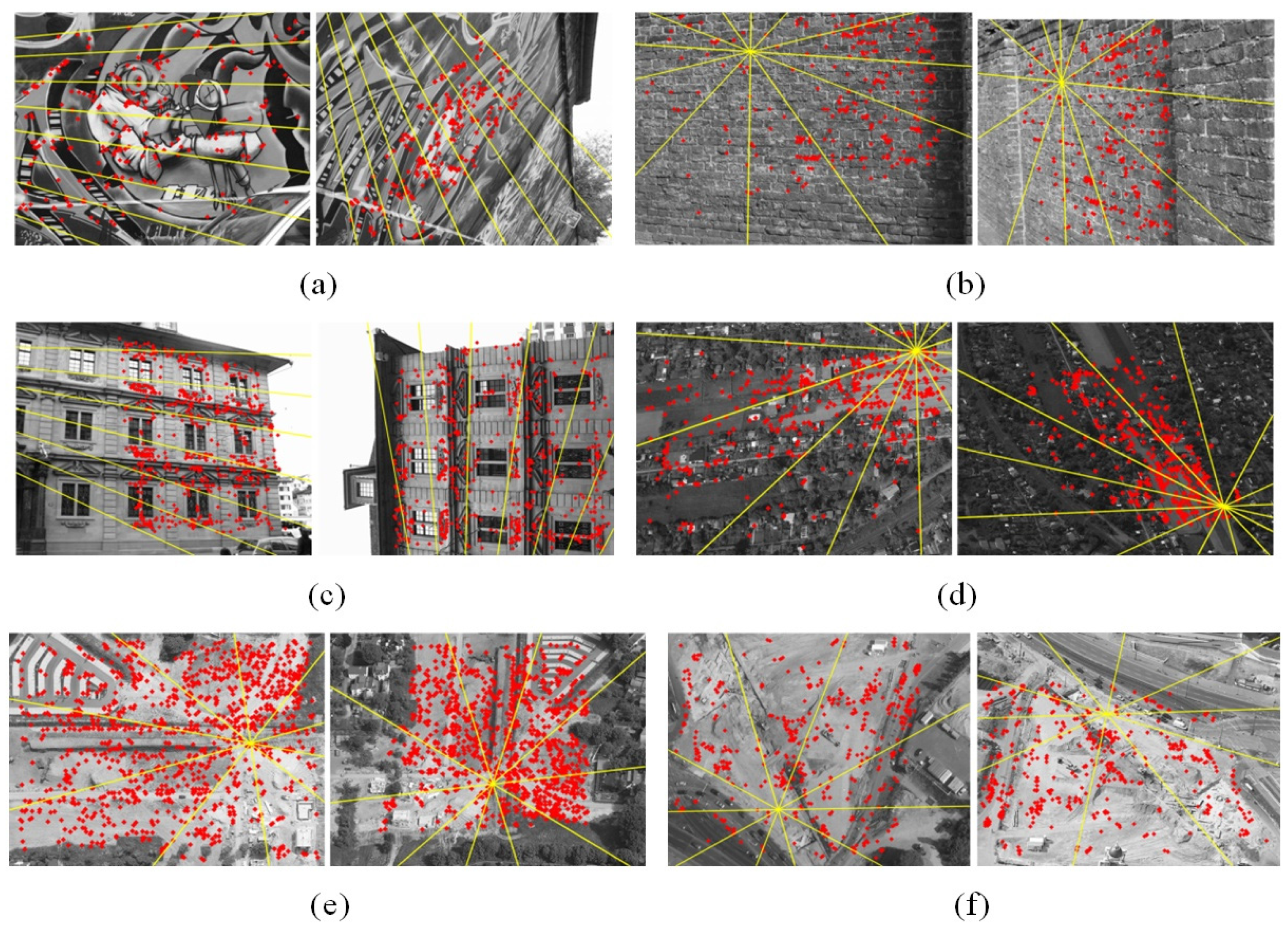
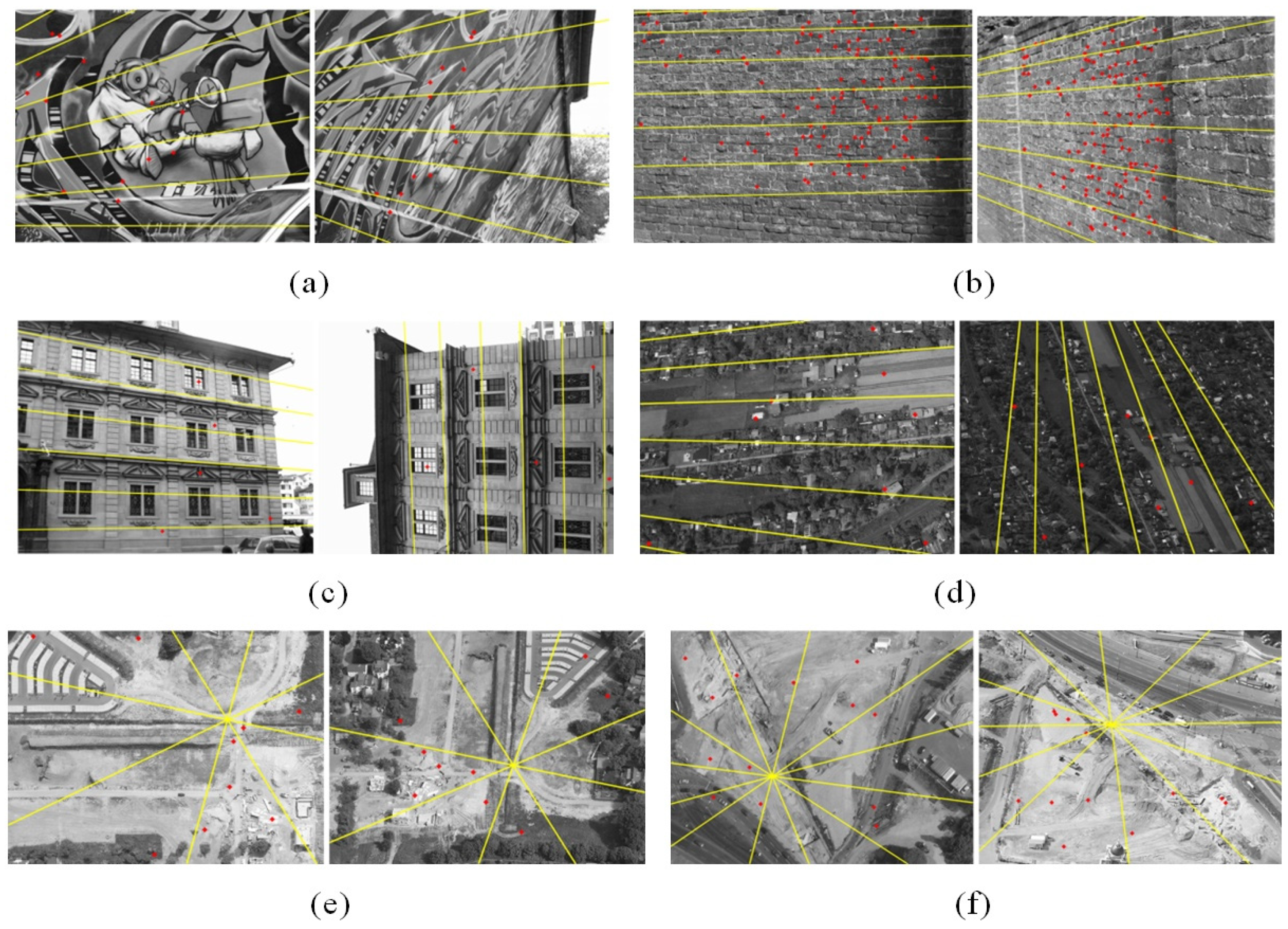
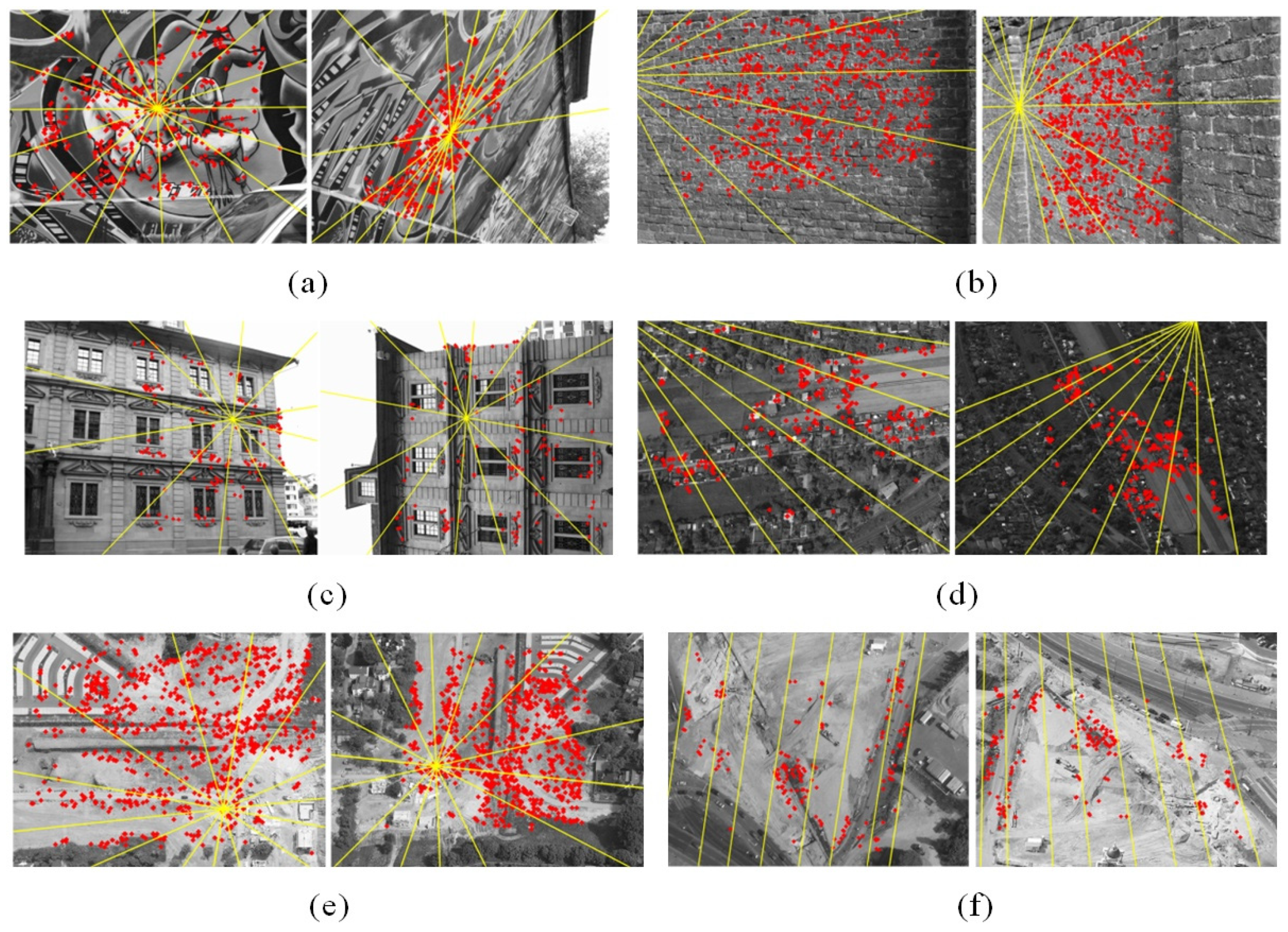
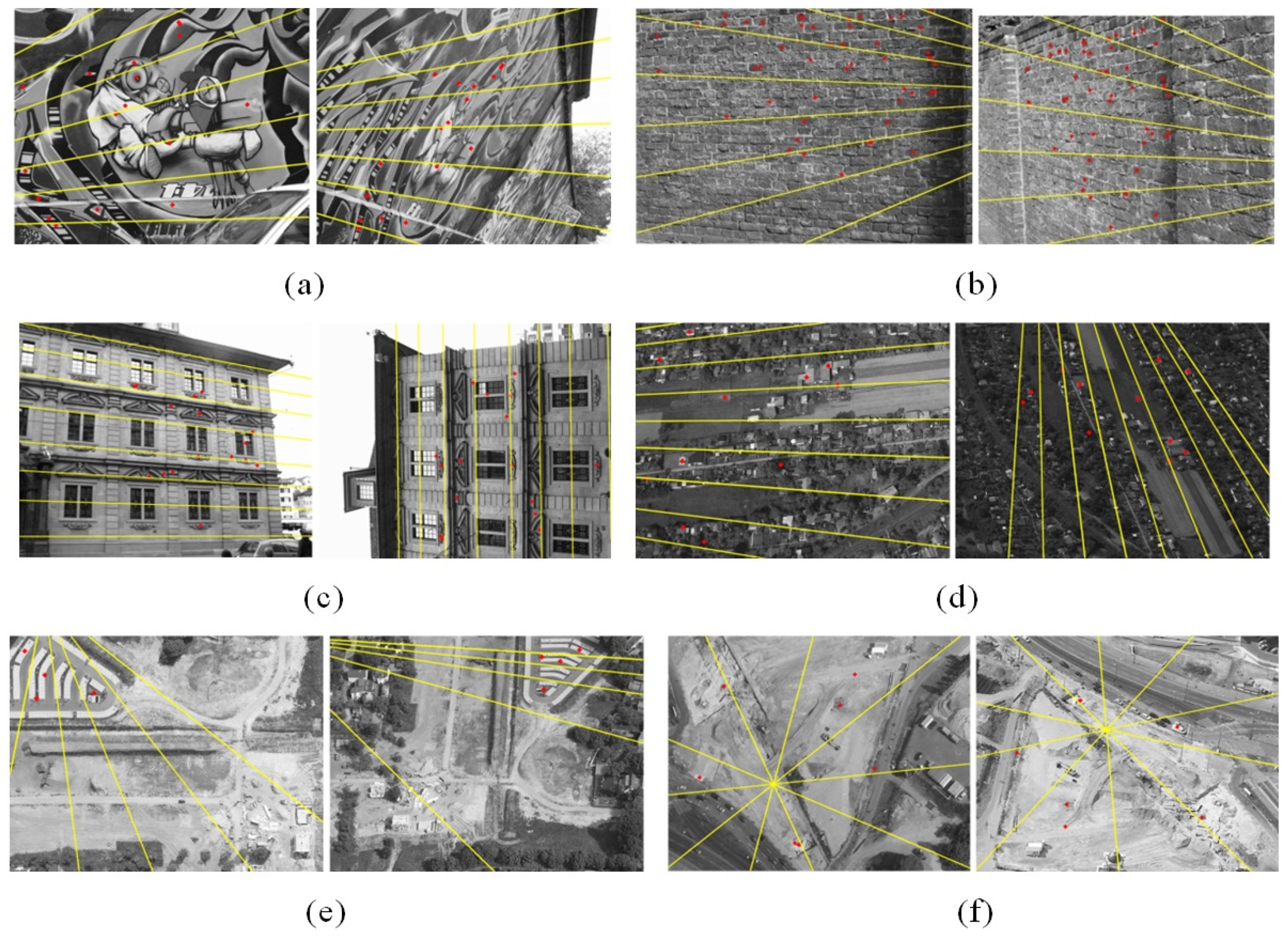
• The proposed method.
• Detone’s method [26]: This approach uses a fully convolutional neural network (MagicPoint) trained on an extensive synthetic dataset which poses a liability to real scenarios. The homographic adaptation (HA) strategy is employed to transform MagicPoint into SuperPoint, which boosts the performance of the detector and generate repeatable feature points. This method also combines SuperPoint with a descriptor subnetwork that generates 256 dimensional descriptors. Matching is achieved using NNDR metric. While the use of HA outperforms classical detectors, the random nature of the HA step limits the invariance of this technique to geometric deformations.
• Morel’s method [10]: This method samples stereo images by simulating discrete poses in the 3D affine space. It uses SIFT algorithm to simulated image pairs and transforms all matches to the original image pair. This method was shown to find correspondences from image pairs with large viewpoint changes. However, false positives often occur for repeating patterns.
• Matas’s method [12]: The approach extracts features using MSER and estimates SIFT descriptors after normalizing the feature points. It uses the NNDR metric to obtain matching features.

In our comparisons, for fair and objective evaluation, a unified strategy was employed for all four methods to eliminate the controversial mismatches. The results are organized as separate figures for each technique. In Figure 8, we provide additional visualization to demonstrate the feature matching results using our method, where the corresponding features and regions around them are denoted by cyan ellipses and lines. Figure 9, Figure 10, Figure 11 and Figure 12 show the final matching results respectively by the methods of proposed, Detone’s, Morel’s and Matas’s, where the red points are matches, and the yellow lines are the estimated epipolar lines. To visually check the matching accuracy for all four methods, we superimpose stereo images based on affine transform, and present the chessboard registration of image pair A using four methods in Figure 13. In Figure 14, we show the contrast of matching error before and after DLT-LSM. Based on the four methods,

Table 7. Quantitative comparison of four methods based on six groups of image pairs. In this table, $n_{{\epsilon }_0}$ is the number of correct matches (pair), β is the correct ratio (%) of matches, ${\epsilon }_{\mathrm{RMSE}}$ is the matching error (pixels), MDQ is the matching distribution quality, t is the total test time (second), and η is the matching efficiency (the unit is second per pair of matching points). The best score of each index is displayed in a bold number.

Method	Indexes	A	B	C	D	E	F
Proposed	$n_{{\epsilon }_0}$	152	349	662	397	972	408
	β	94.43	87.70	87.45	92.98	94.71	90.66
	${\epsilon }_{\mathrm{RMSE}}$	0.64	0.61	0.93	0.54	0.59	0.91
	MDQ	0.893	1.021	1.130	0.988	0.764	1.104
	t	31.49	36.55	45.73	44.61	52.32	43.80
	η	0.196	0.092	0.060	0.105	0.051	0.097
Detone’s	$n_{{\epsilon }_0}$	6	56	0	0	0	0
	β	46.15	43.75	0	0	0	0
	${\epsilon }_{\mathrm{RMSE}}$	3.32	2.28	221.83	53.62	50.25	247.41
	MDQ	1.706	1.290	3.379	2.561	3.027	2.643
	t	16.84	20.33	27.89	24.30	30.95	25.19
	η	1.295	0.159	3.984	3.038	3.095	1.679
Morel’s	$n_{{\epsilon }_0}$	257	408	86	66	532	31
	β	36.25	41.17	23.50	21.71	38.89	13.78
	${\epsilon }_{\mathrm{RMSE}}$	0.91	0.92	1.80	0.96	0.88	0.98
	MDQ	0.974	1.083	1.384	1.920	1.005	1.766
	t	31.38	33.20	33.90	29.13	32.07	33.85
	η	0.044	0.034	0.093	0.096	0.023	0.150
Matas’s	$n_{{\epsilon }_0}$	10	48	7	6	4	0
	β	34.48	78.69	41.18	42.86	66.67	0
	${\epsilon }_{\mathrm{RMSE}}$	2.74	1.39	3.61	8.35	1.93	25.26
	MDQ	1.562	1.495	2.279	1.981	1.596	2.885
	t	2.78	3.82	5.99	6.72	6.37	6.38
	η	0.095	0.063	0.352	0.480	1.062	0.798

presents the quantitative contrast results, including the number of correct matches, correct ratio of matches, matching error, matching distribution quality, matching runtime, and matching efficiency. Considering the training and testing are independent of each other on deep learning, we thus only count the runtime of testing for our and Detone’s method in Table 7.

4. Discussion

4.1. Discussion on Experimental Results of the Key Steps of the Proposed Method

Our overall goal is to automatically produce adequate matches at a subpixel-level from large baseline oblique stereo images. The proposed method reaches the goal by three key steps. First, the proposed IHesAffNet can extract abundant and well-distributed affine invariant regions, laying the good foundation not only for the feature description but also for the DLT-LSM. Second, we design the MTHardNets descriptor based on HardNet, but our improved has better discrimination when compared to HardNet. Third, each correspondence is further optimized based on the DLT-LSM iteration, which is the key to achieving subpixle matching. As can be observed from Table 5, the proposed method outperforms all other methods including AMD and IHD. This is due to the fact that we apply the IHesAffNet in the feature detection stage, instead of using the AffNet. The quality of the feature descriptor also significantly affects the matching performance. The Table 5 also shows that the ISD produces the fewest correct correspondences among the compared six methods. This is attributed to the fact that ISD adopts the SIFT method to extract descriptors, while others generate deep learning-based descriptors; we can use this observation to conjecture that the deep learning strategy generally provides better descriptors when compared to the handcrafted SIFT method. According to the comparison between IHD and the proposed in Table 5, it reveals that our MTHardNets can outperform the HardNet in the process of generating correct matches. Table 6 reveals that the ISD takes the least time among the six methods. This is because the deep leaning-based descriptor would cost more time than handcrafted SIFT descriptor. Figure 7 verifies that the IMN without DLT-LSM step achieves more than 1.5 pixels accuracy and has the lowest correct ratio of matches. That means our DLT-LSM effectively decreases the matching error of deep learning from pixel-level to subpixel-level. In short, according to the contrasting results of the key steps, our proposed method can obtain the most number of correct matches and the highest correct ratio, and synchronously gain the best matching accuracy, which can be attributed to the fact that we have adopted the relatively effective strategy in each stage of the proposed pipeline.

4.2. Discussion on Experimental Results of Comparison Methods

A large number of correct corresponding features with better spatial distribution can be achieved by the proposed deep learning affine invariant feature matching. In the six groups of Large baseline oblique stereo images with repetitive patterns, the numbers of correct corresponding deep learning features are computed as 165, 404, 1504, 545, 1233, and 710, respectively, (see Figure 8). Therefore, these matches would lay a good foundation for estimating the geometry transform between the two images. However, the positional errors of these correspondences before applying DLT-LSM operation are generally more than one pixel (see Figure 14), so it is difficult to produce subpixel matches only by deep learning pipeline.

Table 7 shows that our matching accuracy of six groups of image pairs is at a subpixel-level. As a result, the subpixel accuracy provides better registration between matching features (see Figure 13a). Figure 14 depicts that the feature matching error can be effectively compensated by our DLT-LSM iteration in spite of severe distortion between corresponding neighborhoods. This is because our deep learning feature correspondences would provide good initial transform for the DLT-LSM step. However, there are still a few feature-point matches that DLT-LSM does not work (see Figure 14). We investigate the main reason that these outliers are often located in image regions with poor texture.

The proposed method can obtain sufficient number of conjugate points with the best spatial distribution among the four methods. By the visual inspection of Figure 9, our method gains the most evenly distributed results than the other three methods. According to the quantitative comparison given in Table 7, we can see that our method has advantage in term of matching distribution quality. This is because we have integrated IHesAffNet with MTHardNets, which may contribute to a better matching distribution. The loss function used in Detone’s method only considers the distance between positive samples, which limits the discrimination of the deep learning descriptors, and results in a not well-distributed feature matches (see Figure 10).

Table 7 shows the proposed method has superiority in term of matching correct ratio. Moreover, the detailed view in Figure 13 reveals that our registration is more precise than the other three approaches. Table 7 shows Detone’s method fails to obtain correct matches from image pairs C, D, E and F. The main reason may be that the homographic adaptation of SuperPoint is randomly, which limits its invariance to diverse geometric deformations.

Observing the matching efficiency in Table 7, our proposed is more efficient than the Detone’s. The main reason is that our method would stably gain a large number of matches, while the Detone’s method almost fails to obtain matches from large oblique stereo images. However, the matching efficiency of our proposed and Detone’s are not as good as the handcrafted methods of Morel’s and Matas’s. This is because the deep leaning methods involve numerous convolution operations in the process of feature detection and description.

According to the aforementioned qualitative and quantitative results, the proposed approach is superior in terms of number of correct matches, correct ratio of matches, matching accuracy, and distribution quality. The contribution of our method includes three aspects. The first is the proposed IHesAffNet can detect more well-distributed features with higher repeatability than the original AffNet. The second is the proposed MTHardNets can generate higher discrimination descriptor when compared to HardNet especially for the poor texture image regions. The third is the advanced DLT-LSM can significantly improve the accuracy of corresponding points. In summary, our method is effective and stable for large baseline oblique stereo image matching.

5. Conclusions

In this paper, we presented a novel and effective end-to-end feature matching pipeline for large baseline oblique stereo images with complex geometric and radiometric distortions as well as repetitive patterns. The proposed introduces the IHesAffNet that can extract affine invariant features with well distribution and good repeatability. The output of this network inputs to the proposed MTHardNets that generates highly discriminatory descriptors providing increased accuracy for stereo feature matching. Furthermore, the proposed approach features a DLT-LSM based iterative step that compensates for the position errors of feature points. As a result, it can obtain a sufficient number of subpixel-level matches with uniform spatial distribution. The qualitative and quantitative comparisons on different large baseline oblique images verify that our method can outperforms the state-of-the-art methods for oblique image matching. Future research can include developing deep learning strategies for multiple image primitives, such as corner, edges, and regions. Moreover, the affine invariant matching approach can be extended from planar scenes to large baseline oblique 3D scenes. Meanwhile, the proposed end-to-end CNN can be extended from grayscale images to color images for application.

References

1. Qin, R. A critical analysis of satellite stereo pairs for digital surface model generation and a matching quality prediction model. ISPRS J. Photogramm. Remote Sens. 2019, 154, 139–150. [Google Scholar] [CrossRef]
2. Liu, W.; Wu, B. An integrated photogrammetric and photoclinometric approach for illumination-invariant pixel-resolution 3D mapping of the lunar surface. ISPRS J. Photogramm. Remote Sens. 2020, 159, 153–168. [Google Scholar] [CrossRef]
3. Zhang, H.; Ni, W.; Yan, W.; Xiang, D.; Bian, H. Registration of multimodal remote sensing image based on deep fully convolutional neural network. IEEE J. Stars 2019, 12, 3028–3042. [Google Scholar] [CrossRef]
4. Gruen, A. Development and status of image matching in photogrammetry. Photogramm. Rec. 2012, 27, 36–57. [Google Scholar] [CrossRef]
5. Song, W.; Jung, H.; Gwak, I.; Lee, S. Oblique aerial image matching based on iterative simulation and homography evaluation. Pattern Recognit. 2019, 87, 317–331. [Google Scholar] [CrossRef]
6. Lowe, D.G. Distinctive image features from scale-invariant keypoints. Int. J. Comput. Vis. 2004, 60, 91–110. [Google Scholar] [CrossRef]
7. Bay, H.; Ess, A.; Tuytelaars, T.; Gool, L. Speeded-Up robust features (SURF). Comput. Vis. Image Underst. 2008, 110, 346–359. [Google Scholar] [CrossRef]
8. Murartal, R.; Montiel, J.; Tardos, J. ORB-SLAM: A versatile and accurate monocular SLAM system. IEEE Trans. Robot. 2015, 31, 1147–1163. [Google Scholar] [CrossRef] [Green Version]
9. Ma, W.; Wen, Z.; Wu, Y.; Jiao, L.; Gong, M.; Zheng, Y.; Liu, L. Remote sensing image registration with modified SIFT and enhanced feature matching. IEEE Geosci. Remote Sens. Lett. 2017, 14, 3–7. [Google Scholar] [CrossRef]
10. Morel, J.M.; Yu, G.S. ASIFT: A new framework for fully affine invariant image comparison. SIAM J. Imaging Sci. 2009, 2, 438–469. [Google Scholar] [CrossRef]
11. Mikolajczyk, K.; Schmid, C. Scale & affine invariant interest point detectors. Int. J. Comput. Vis. 2004, 60, 63–86. [Google Scholar] [CrossRef]
12. Matas, J.; Chum, O.; Urban, M.; Pajdla, T. Robust wide-baseline stereo from maximally stable extremal regions. Image Vis. Comput. 2004, 22, 761–767. [Google Scholar] [CrossRef]
13. Liu, X.; Samarabandu, J. Multiscale Edge-Based Text Extraction from Complex Images. In Proceedings of the IEEE International Conference on Multimedia and Expo, Toronto, ON, Canada, 9–12 July 2006; pp. 1721–1724. [Google Scholar] [CrossRef] [Green Version]
14. Tuytelaars, T.; Gool, L. Matching widely separated views based on affine invariant regions. Int. J. Comput. Vis. 2004, 59, 61–85. [Google Scholar] [CrossRef]
15. Yao, G.; Man, X.; Zhang, L.; Deng, K.; Zheng, G. Registrating oblique SAR images based on complementary integrated filtering and multilevel matching. IEEE J. Stars. 2019, 12, 3445–3457. [Google Scholar] [CrossRef]
16. Mikolajczyk, K.; Tuytelaars, T.; Schmid, C.; Zisserman, A.; Matas, J.; Schaffalitzky, F.; Kadir, T.; Gool, L. A comparison of affine region detectors. Int. J. Comput. Vis. 2005, 65, 43–72. [Google Scholar] [CrossRef] [Green Version]
17. Mikolajczyk, K.; Schmid, C. A performance evaluation of local descriptors. IEEE Trans. Pattern Anal. 2005, 27, 1615–1630. [Google Scholar] [CrossRef] [PubMed] [Green Version]
18. Lenc, K.; Vedaldi, A. Learning covariant feature detectors. In Proceedings of the ECCV Workshop on Geometry Meets Deep Learning, Amsterdam, The Netherlands, 31 August–1 September 2016; pp. 100–117. [Google Scholar] [CrossRef] [Green Version]
19. Zhang, X.; Yu, F.X.; Karaman, S. Learning discriminative and transformation covariant local feature detectors. In Proceedings of the IEEE Conference on Computer Vision and Pattern Recognition (CVPR), Honolulu, HI, USA, 21–26 July 2017; pp. 4923–4931. [Google Scholar] [CrossRef]
20. Doiphode, N.; Mitra, R.; Ahmed, S. An improved learning framework for covariant local feature detection. In Proceedings of the Asian Conference on Computer Vision (ACCV), Perth, Australia, 2–6 December 2018; pp. 262–276. [Google Scholar] [CrossRef] [Green Version]
21. Yi, K.M.; Verdie, Y.; Fua, P.; Lepetit, V. Learning to assign orientations to feature points. In Proceedings of the IEEE Conference on Computer Vision and Pattern Recognition (CVPR), Las Vegas, NV, USA, 26 June–1 July 2016. [Google Scholar] [CrossRef] [Green Version]
22. Detone, D.; Malisiewicz, T.; Rabinovich, A. Superpoint: Self-supervised interest point detection and description. In Proceedings of the IEEE Conference on Computer Vision and Pattern Recognition Workshops, Salt Lake City, UT, USA, 18–22 June 2018; pp. 224–236. [Google Scholar] [CrossRef] [Green Version]
23. Tian, Y.; Fan, B.; Wu, F. L2-Net: Deep Learning of Discriminative Patch Descriptor in Euclidean Space. In Proceedings of the IEEE Conference on Computer Vision and Pattern Recognition (CVPR), Honolulu, HI, USA, 21–26 July 2017; pp. 6128–6136. [Google Scholar] [CrossRef]
24. Mishchuk, A.; Mishkin, D.; Radenovic, F. Working hard to know your neighbor’s margins: Local descriptor learning loss. In Proceedings of the Neural Information Processing Systems, Long Beach, CA, USA, 4–9 December 2017; pp. 4826–4837. [Google Scholar]
25. Mishkin, D.; Radenovic, F.; Matas, J. Repeatability is not Enough: Learning Affine Regions via Discriminability. In European Conference on Computer Vision (ECCV); Springer: Cham, Switzerland, 2018; pp. 287–304. [Google Scholar] [CrossRef] [Green Version]
26. Wan, J.; Yilmaz, A.; Yan, L. PPD: Pyramid patch descriptor via convolutional neural network. Photogramm. Eng. Remote Sens. 2019, 85, 673–686. [Google Scholar] [CrossRef]
27. Han, X.; Leung, T.; Jia, Y.; Sukthankar, R. MatchNet: Unifying feature and metric learning for patch-based matching. In Proceedings of the IEEE Conference on Computer Vision and Pattern Recognition (CVPR), Boston, MA, USA, 7–12 June 2015; pp. 3279–3286. [Google Scholar] [CrossRef] [Green Version]
28. Hoffer, E.; Ailon, N. Deep metric learning using triplet network. In Proceedings of the International Conference on Learning Representations, San Diego, CA, USA, 7–9 May 2015; pp. 84–92. [Google Scholar] [CrossRef] [Green Version]
29. Tian, Y.; Yu, X.; Fan, B. SOSNet: Second order similarity regularization for local descriptor learning. In Proceedings of the Computer Vision and Pattern Recognition, Long Beach, CA, USA, 16–20 June 2019; pp. 11016–11025. [Google Scholar] [CrossRef] [Green Version]
30. Ebel, P.; Trulls, E.; Yi, K.M.; Fua, P.; Mishchuk, A. Beyond Cartesian Representations for Local Descriptors. In Proceedings of the International Conference on Computer Vision (ICCV), Seoul, Korea, 27 October–2 November 2019; pp. 253–262. [Google Scholar] [CrossRef] [Green Version]
31. Luo, Z.; Shen, T.; Zhou, L.; Zhu, S.; Zhang, R.; Yao, Y.; Fang, T.; Quan, L. GeoDesc: Learning local descriptors by integrating geometry constraints. In Proceedings of the European Conference on Computer Vision (ECCV), Munich, Germany, 8–14 September 2018; pp. 170–185. [Google Scholar] [CrossRef] [Green Version]
32. Luo, Z.; Shen, T.; Zhou, L.; Zhu, S.; Zhang, R.; Yao, Y.; Fang, T.; Quan, L. ContextDesc: Local descriptor augmentation with cross-modality context. In Proceedings of the IEEE Conference on Computer Vision and Pattern Recognition (CVPR), Long Beach, CA, USA, 16–20 June 2019; pp. 2527–2536. [Google Scholar] [CrossRef] [Green Version]
33. Yi, K.; Trulls, E.; Lepetit, V.; Fua, P. LIFT: Learned invariant feature transform. In Proceedings of the European Conference on Computer Vision (ECCV), Amsterdam, The Netherlands, 11–14 October 2016; pp. 467–483. [Google Scholar] [CrossRef] [Green Version]
34. Ono, Y.; Trulls, E.; Fua, P. LF-Net: Learning local features from images. In Proceedings of the Neural Information Processing Systems, Montreal, QC, Canada, 3–8 December 2018; pp. 6234–6244. [Google Scholar]
35. Revaud, J.; Weinzaepfel, P.; De, S. R2D2: Repeatable and reliable detector and descriptor. arXiv 2019, arXiv:1906.06195. [Google Scholar]
36. Jin, Y.; Mishkin, D.; Mishchuk, A.; Matas, J.; Fua, P.; Yi, F.; Trulls, E. Image matching across wide baselines: From paper to practice. Int. J. Comput. Vis. 2020, 1–31. [Google Scholar] [CrossRef]
37. Sedaghat, A.; Mokhtarzade, M.; Ebadi, H. Uniform robust scale-invariant feature matching for optical remote sensing images. IEEE Trans. Geosci. Remote Sens. 2011, 49, 4516–4527. [Google Scholar] [CrossRef]
38. Zhu, Q.; Wu, B.; Xu, Z.X. Seed point selection method for triangle constrained image matching propagation. IEEE Geosci. Remote Sens. Lett. 2006, 3, 207–211. [Google Scholar] [CrossRef]
39. Brown, M.; Lowe, D.G. Automatic panoramic image stitching using invariant features. Int. J. Comput. Vis. 2007, 74, 59–73. [Google Scholar] [CrossRef] [Green Version]
40. Paszke, A.; Gross, S.S.; Chintala, G.; Chanan, E.; Yang, Z.; DeVito, Z.; Lin, A.; Desmaison, L.; Lerer, A. Automatic differentiation in pytorch. In Proceedings of the Advances in Neural Information Processing Systems Workshop, Long Beach, CA, USA, 4–9 December 2017. [Google Scholar]
41. Podbreznik, P.; Potočnik, B. A self-adaptive ASIFT-SH method. Adv. Eng. Inform. 2013, 27, 120–130. [Google Scholar] [CrossRef]
Figure 1. Flow chart of the proposed approach.
Remotesensing 13 00274 g001
Figure 2. Matching performances of multiple versions of AffNet with different configurations, where AffNet6 provides the best result.
Remotesensing 13 00274 g002
Figure 3. Comparison between the AffNet and IHesAffNet on the Graf1-6 stereo image dataset. (a,c) are the detecting results by the AffNet and IHesAffNet, respectively; (b,d) are the verifiable tests based on the detection of (a,c), respectively. The yellow and cyan ellipses respectively denote the detected and matched features. Note that the bottom row that corresponds to our approach is better.
Remotesensing 13 00274 g003
Figure 4. Schematic of the MTHardNets with K nearest negative samples using the EWLF, where (K + 2) image patches are parallelly fed into the same HardNet, then the matching descriptors ( R i ,   P i ) and non-matching descriptors ( N i 1 st , , N i K th ) are respectively outputted. The Lu and wu represent the loss and weight, respectively, and the EWLF can be expressed by L given in Equations (6) and (7).
Remotesensing 13 00274 g004
Figure 5. The MDD comparison among 564 groups of (w1, w2, w3) with uniform sampling.
Remotesensing 13 00274 g005
Figure 6. The discrimination comparison between proposed MTHardNets and HardNet descriptors by using five pairs of matching points. The PDD is the abbreviation for positive descriptor distance and NDD for negative descriptor distance.
Remotesensing 13 00274 g006
Figure 7. Comparison of different matching method in terms of the (a) correct ratio β (%) of matches (higher values are better) and (b) root mean square error ε RMSE (pixels) of matches (lower values are better).
Remotesensing 13 00274 g007
Figure 8. (af) Matching results of our approach on a group of stereo pairs. The ellipses represent the regions matching around each feature point. Lines represent the matches.
Remotesensing 13 00274 g008
Figure 9. (af) Red points show the matching results of the proposed method with groups of stereo images. The yellow lines represent the epipolar lines estimated from matching points.
Remotesensing 13 00274 g009
Figure 10. (af) Red points show the matching results of the Detone’s method with groups of stereo images. The yellow lines represent the epipolar lines estimated from matching points.
Remotesensing 13 00274 g010
Figure 11. (af) Red points show the matching results of the Morel’s method with groups of stereo images. The yellow lines represent the epipolar lines estimated from matching points.
Remotesensing 13 00274 g011
Figure 12. (af) Red points show the matching results of the Mata’s method with groups of stereo images. The yellow lines represent the epipolar lines estimated from matching points.
Remotesensing 13 00274 g012
Figure 13. The chessboard registration results of four comparison approaches for image pair A. (a) Registration image of proposed, (b) registration image of Detone’s, (c) registration image of Morel’s, and (d) registration image of Matas’s. Subregions I and II display the detailed view.
Remotesensing 13 00274 g013
Figure 14. Contrast of the affine transform error before and after DLT-LSM for the proposed approach. For intuition, both (a) and (b) present 10 random sample features of the matching, which are respectively extracted from image pairs A and D.
Remotesensing 13 00274 g014