Article

Fusion and Correction of Multi-Source Land Cover Products Based on Spatial Detection and Uncertainty Reasoning Methods in Central Asia

1
College of Geoscience and Surveying Engineering, China University of Mining and Technology, Beijing 100083, China
2
Key Laboratory of Land Surface Pattern and Simulation, Institute of Geographic Sciences and Natural Resources Research, Chinese Academy of Sciences, Beijing 100101, China
*
Author to whom correspondence should be addressed.
Remote Sens. 2021, 13(2), 244; https://doi.org/10.3390/rs13020244
Submission received: 15 December 2020 / Revised: 9 January 2021 / Accepted: 10 January 2021 / Published: 12 January 2021

Abstract

:
Land cover products are an indispensable data source in land surface process research, and their accuracy directly affects the reliability of related research. Due to the differences in factors such as satellite sensors, the temporal–spatial resolution of remote sensing images, and landcover interpretation technologies, various recently released land cover products are inconsistent, and their accuracy is usually insufficient to meet application requirements. This study, therefore, established a fusion and correction method for multi-source landcover products by combining them with landcover statistics from the Food and Agriculture Organization of the United Nations (FAO), introducing a spatial consistency discrimination technique, and applying an improved Dempster-Shafer evidence fusion method. The five countries in Central Asia were used for a method application and verification assessment. The nine products selected (CCI-LC, CGLS, FROM-GLC, GLCNMO, MCD12Q, GFSAD30, PALSAR, GSWD, and GHS-BUILT) were consistent in time and covered the study area. Based on the interpretation of 1437 high-definition image verification areas, the overall accuracy of the fusion landcover result was 85.32%, and the kappa coefficient was 0.80, which was better than that of the existing comprehensive products. The spatial consistency fusion method had the advantage of an improved statistical fitting, with an overall similarity statistic of 0.999. The improved Dempster-Shafer evidence theory fusion method had an accuracy that was 4.86% higher than the spatial consistency method, and the kappa coefficient increased by 0.07. Combining these two methods improved the consistency of the multi-source data fusion and correction method established in this paper and will also provide more reliable basic data for future research in Central Asia.

Graphical Abstract

1. Introduction

Landcover (use) changes affect the structure and function of ecosystems and other land surface processes and are indispensable basic data for studies of ecosystem evaluation [1], landscape pattern simulation [2], vegetation phenology monitoring [3], and carbon sink simulation research [4]. With the rapid development of satellite remote sensing technology, the use of remote sensing images has become the most popular method for large-scale landcover mapping. Since the land-use and landcover change project was proposed by the International Geosphere and Biosphere Plan in 1995, major geoscience research institutions around the world have successively developed a variety of landcover products with different scales and resolutions based on satellite remote sensing images [5]. There are now more than 20 sets of global scale and 40 sets of intercontinental or national scale landcover mapping products [6,7]. Landcover products can be divided into composite and single types, such as the International Geosphere-Biosphere Program Data and Information System Cover (IGBP-DISCover) developed by the United States Geological Survey (USGS), Global Land Cover 2000 (GLC2000) developed by the European Commission Joint (ECJRC), Global Land Cover Map (GlobCover) and Climate Change Initiative Land Cover (CCI-LC) developed by the European Space Agency (ESA), Finer Resolution Observation and Monitoring—Global Land Cover (FROM-GLC) developed by Tsinghua University in China, and GlobeLand30 developed by the National Basic Geographic Information Center of China [8]. In addition to the comprehensive landcover products, research institutions have also produced single-type landcover products, such as the cropland product Global Food Security—support analysis data 30 m (GFSAD30) developed by USGS [9] and the forest landcover product Advanced Land Observing Satellite Phased Array L-band SAR (PALSAR) developed by the Japan Aerospace Exploration Agency (JAXA) [10]. However, the differences among satellite operation, sensor types, classification methods, and verification methods have resulted in a large inconsistency among the landcover products from different data sources. Consequently, the accuracy cannot always meet application requirements [11]. Low precision landcover data will result in greater errors in applications, leading to greater uncertainty in the research results. Therefore, it is of great significance to integrate existing multi-source landcover data and improve data accuracy [12,13].
A variety of methods have been proposed for the fusion and correction of multi-source landcover data. Based on the principle of evidence convergence, Jung et al. used affinity scores and fuzzy consistency methods to fuse Global Land Cover Characterization (GLCC), GLC2000, and Moderate Resolution Imaging Spectroradiometer (MODIS) data to generate comprehensive landcover products with improved characteristics [14]. Bai et al. fused the MODIS Vegetation Continuous Fields (VCF), MODIS Cropland Probability, and Advanced Very-High-Resolution Radiometer (AVHRR) Continuous Fields of Tree Cover (CFTC) datasets based on fuzzy logic to obtain global 1 km landcover fusion data [15]. These studies applied the method of assigning definition rules for multi-source data fusion, in addition to quantitative methods based on statistics. Fritz et al. used statistics to calibrate on the basis of determining the type of product sorting possibilities, and fused GLC-2000, MODIS land cover, GlobCover, MODIS crop likelihood, and AfriCover dataset from the Food and Agriculture Organization (AfriCover) to obtain a 1 km resolution cropland map of Africa [16]. According to the consistency between different remote sensing data and statistics, Dmitry et al. merged GLC2000, VCF, Vegetation Fraction (VF), and Geographic Information System (GIS) data to generate 1 km resolution landcover data for Russia [17]. Based on the best consistency level and product combination, Lu et al. used statistics as constraints to integrate GlobeLand 30, CCI-LC, GlobCover2009, MODIS Collection 5 (MODIS C5), and MODIS cropland to generate 500 m resolution arable landcover data for China [18]. These studies showed that the fusion of multi-source landcover data could improve data accuracy. However, fusion based solely on fuzzy theory is highly subjective, while fusion based only on a consistency analysis produces greater uncertainty in regions with low consistency. In addition, with advances in technology, many high-precision single landcover products have emerged. Therefore, how to develop the advantages of these two techniques and also effectively integrate comprehensive and single-type landcover products are the keys to improve the fusion accuracy of multi-source landcover products.
The Dempster-Shafer evidence theory is an evidence-based fusion method proposed by Dempster and improved by Shafer [19,20]. It can deal with the uncertainties caused by randomness and ambiguity. Unlike Bayesian probability theory, it does not require a prior probability density and is therefore widely utilized in artificial intelligence and multi-source information fusion [21]. Ran et al. merged GIS data with Moderate Resolution Imaging Spectroradiometer Land Cover Map in 2001 (MOD12Q1) based on evidence theory to obtain 1 km resolution landcover data for China in 2000 [22]. Based on this theoretical framework, Song et al. integrated products such as GlobCover, MODIS, GLC2000, and Global Land Cover by National Mapping Organizations (GLCNMO) covering China and produced landcover data for use in China’s land cover classification system (LCCS) in 2005 [23]. When there is a high degree of conflict between the available evidence, the regularization process during the synthesis of evidence theory may lead to the “Zedeh” paradox. This states that even if most of the evidence supports proposition A, the result is that the synthesized proposition A is also negated as long as one piece of evidence denies proposition A, which leads to the evidence being affirmed by the proposition that was negated by the majority of evidence; thus, forming a paradox [24]. Researchers worldwide are committed to improving the Dempster-Shafer evidence theory algorithm [25,26], but few studies have applied the results to the integration of landcover products.
In this study, a spatial consistency analysis was introduced with an improved Dempster-Shafer evidence fusion theory and then a landcover fusion and correction method was established for comprehensive and single type products combined with the Food and Agriculture Organization of the United Nations (FAO) statistics. First, we performed a spatial consistency discriminant analysis on nine landcover products to extract regions with high spatial consistency. Then we used the improved Dempster-Shafer theory for data fusion and filled in the results for regions with lower spatial consistency. This method can effectively avoid the uncertainty that occurs when the spatial consistency is low. Central Asia was selected as the research area to apply and verify the proposed method.

2. Data and Methods

2.1. Study Area

The five Central Asian countries (Kazakhstan, Kyrgyzstan, Tajikistan, Turkmenistan, and Uzbekistan) in this study are located in the middle of the Eurasian continent (35°N~55°N, 46°E~85°E), which has a temperate continental drought and semi-arid climate, with little precipitation and strong evaporation (Figure 1) [27]. The total area is about 4 × 10⁶ km2. The western and central parts of the region are low-lying, and plateaus and mountains occupy the southeast and northwest. Central Asian landscapes are dominated by deserts and grasslands. The main water resources are snow meltwater from mountains and inland lakes, and the area and volume of inland lakes have been greatly reduced due to the dual effects of climate change and human activities [28]. As the Silk Road passes through these countries, which are member states of the Belt and Road region, the study of the ecological environment and surface processes in Central Asia has become an important research topic [29]. However, due to the huge changes in landcover in Central Asia since the disintegration of the Soviet Union, the different time phases of various products, and rough spatial resolution, the uncertainty of remote sensing interpretation has increased, with a lack of clarity among the landcover types in the fragmented landscape [30,31]. Moreover, the landcover data sets currently used in studies of Central Asia are relatively old [32,33]. A number of landcover data sets for the period around 2015 have been released internationally, and these can be used to study the relatively recent landcover distribution characteristics of Central Asia.

2.2. Data Sources and Preprocessing

We used nine landcover products in 2015, namely CCI-LC [34], Copernicus Global Land Service (CGLS) [35,36], FROM-GLC [37,38], GLCNMO [39,40,41,42], Moderate Resolution Imaging Spectroradiometer Land Cover Type Product (MCD12Q) [41,42,43], GFSAD30 [10,44], PALSAR [45,46], Global Surface Water Data (GSWD) [9], and Global Human Settlement Layer Built-up area (GHS-BUILT) [47,48]. There were differences between these products in terms of their spatial resolution, sensors, classification methods, overall accuracy, and classification systems (Table 1). The overall accuracy of the combined landcover products was roughly 60–80%, while the accuracy of a single landcover product could exceed 90%.
Because the resolution of each landcover product was inconsistent, it was necessary to project and resample the data to ensure the area was not deformed when merging. Using the world_cylindrical_equal_area as the benchmark, the nine landcover products were unified into the same geographic coordinate system and projection. Taking into account the inconsistency of the spatial resolution of the above products, which ranged from 25 to 500 m, the mode aggregation method was adopted to upscale the fine resolution products, and the nearest neighbor pixel interpolation approach was applied to downscale the coarse resolution products according to previous studies [49]. The increase of the scale would omit information about the data while decreasing the scale would introduce more uncertainty into the data. The resolutions ranged from 25 to 500 m, but only MCD12Q had a resolution of 500 m, while most products had a resolution of less than 100 m. Therefore, after careful consideration, 300 m was selected as the resolution of the multi-source products after resampling, which can ensure that high-resolution products do not lose much information when merging pixels and can also prevent low-resolution products from generating wrong information when downscaling. This ensured that high-resolution products did not lose much information when merging pixels but also prevented the low-resolution products from generating incorrect information when downscaling.

2.3. Multi-Source Land Cover Data Fusion and Correction Method

We developed a method based on the combination of a spatial consistency analysis and the improved Dempster-Shafer evidence theory (Figure 2). The main steps were as follows. (1) The existing multi-source landcover products were subjected to a unified classification system, spatial referencing, and resolution. (2) Following the collection of FAO statistics, a spatial consistency analysis method was used for data fusion and regions with a higher consistency were extracted. (3) The fusion results from the application of the improved Dempster-Shafer evidence theory were employed to fill the area of low consistency in the spatial consistency method. (4) High-definition image interpretation samples from Google Earth were applied to evaluate the accuracy of the fusion result. A spatial consistency analysis has the advantage of drawing homogeneous areas of large landscapes, and the improved Dempster-Shafer evidence theory fusion method can effectively deal with the uncertainty of low-consistency areas. Therefore, we established a multi-source landcover product fusion and correction method combining the two methods.

2.3.1. Unified Classification System for Multi-Source Land Cover Products

Due to the different production units and sensors, the classification systems and definitions of landcover types were also different for each landcover product. We defined the fusion result as nine classes, and the landcover types of each product were also grouped into nine classes according to the classification system used for the comprehensive landcover products (Table 2). The specific definitions of each single-type product were as follows: GFSAD30 is a single product for cultivated land, in which cultivated land was defined as planted crops and fallow land. Fallow land referred to farmland that had not been cultivated in a season or a year and included planting equipment and plantations (such as orchards, tea gardens, etc.). PALSAR is a single-type product for forest land, which included forest coverage areas with a canopy density ≥10%. GSWD is a single-type product for permanent and seasonal water bodies. If there was water throughout the whole observation period (which was the thawing period), the lake was regarded as a permanent water body. If the area of the lake shrank during the thawing period, the pixels around the lakeside no longer represented water, and the feature was regarded as a seasonal water body. GHS-BUILT is a single-type product for artificial surfaces, namely built-up areas. Built-up areas referred to closed buildings on the ground that were used to shelter humans, animals, and goods or for the production of economic commodities. This category also includes refugee settlements, slums, and other temporary settlements.

2.3.2. Spatial Consistency Analysis

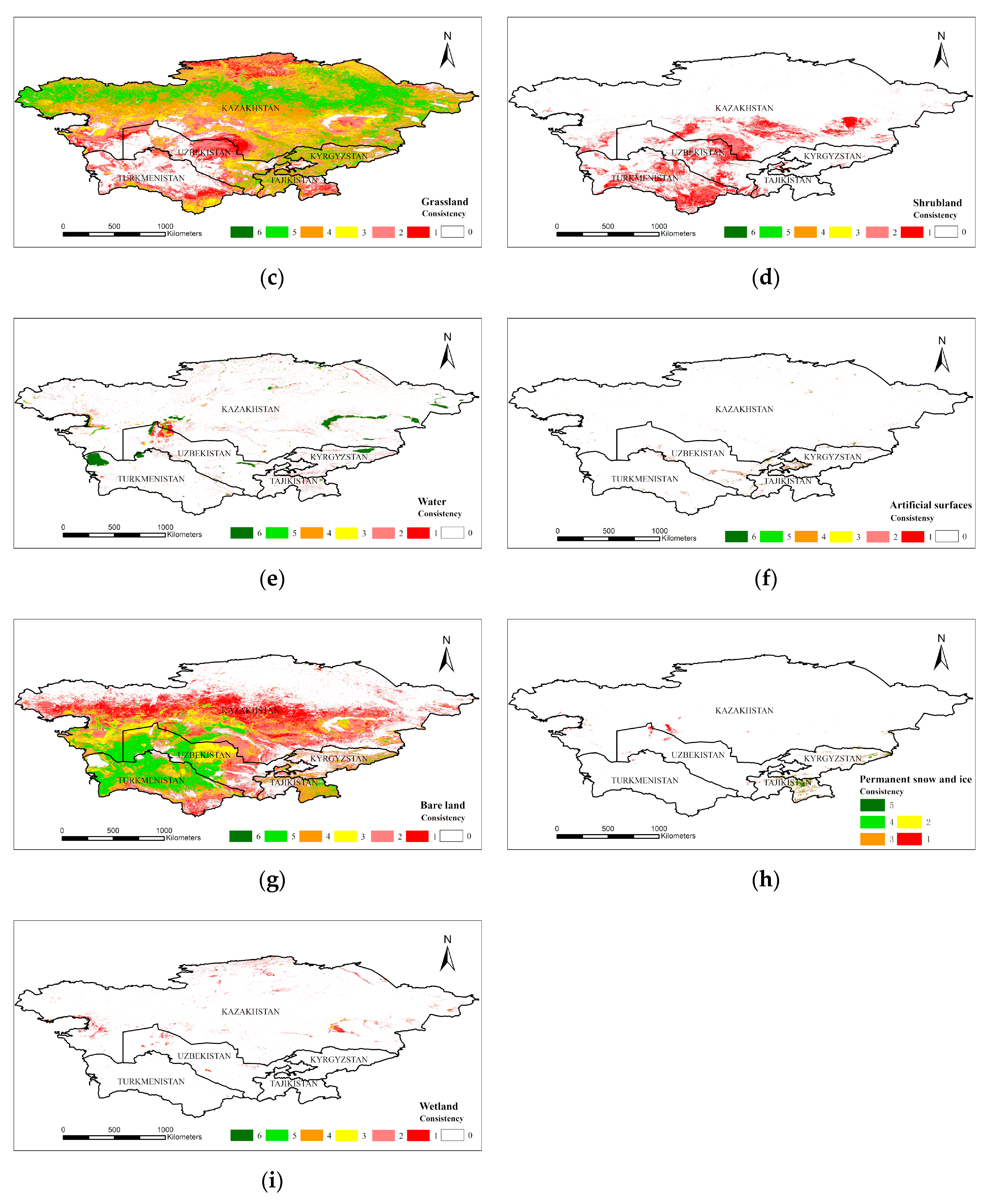
A spatial consistency analysis can accurately express the spatial differentiation of various landcover products [6,18]. We used the spatial analysis tools in ESRI ArcGIS 10.5 Desktop software (CA, USA) to overlay landcover products and counted the number and distribution of pixels for the consistency of each class. The classes which had single-type products were cropland, forest, water bodies, and artificial surfaces, and the number of products was 6. Therefore, the highest consistency of these land types was 6, and the highest consistency of the other land types was 5. The higher the confidence, the higher the probability that the pixel was considered to be the land type, and vice versa. Taking cropland as an example, if all the cropland products represented cropland at the same time, the consistency of cropland in the pixel was 6, which was completely spatially consistent in space, and the likelihood that the pixel was actually cropland was extremely high. If there was no product for which the pixel was cultivated land (i.e., consistency = 0), the possibility that the pixel was cropland was extremely low (Figure 3). Statistics for the area of cropland, forest, grassland, and water in various countries were obtained from the FAO, and the results of each level of integration were compared using statistics. Because statistics were based on the country as a statistical unit, the integration of each country based on the statistics generated more accurate results at the national scale. The area data for various types of landcover were obtained from FAO statistics, solely including cropland, forest, grassland, water bodies, and other areas of each country. Thus, the land types used for comparison with the statistical area in this study were cropland, forest, grassland, and water. Due to the lack of statistics for other landcover types, they are not constrained by statistical area when merging and are superimposed step-by-step according to the level of consistency until all pixels are assigned a category.
The specific operation undertaken when using spatial consistency analysis for data fusion was to overlap each product spatially and then use the raster calculator in ArcGIS software to analyze the consistency of each landcover type. Following this procedure, a class assignment for each grid was performed to obtain a sequence from high to low consistency. For grids with a high degree of confidence (consistency ≥4), each grid was assigned to the class with the highest confidence level, and then the fusion result of the land type was compared with the landcover statistics. If the aggregated area then exceeded the statistically reported value, landcover type areas of lower consistency were not added. If the aggregated area was less than the statistically reported value, landcover type areas of lower consistency were added until the area was equal to or slightly larger than the statistically reported area. In the low-confidence (consistency ≤3) grids, there could be several types of landcover with the highest confidence level at the same time. For example, there were grids with a confidence level of 3 for both cropland and grassland. In this case, a restriction was attached, with the use of a certain single-type product restricted in each level of the consistency analysis. The fusion results of land types were continuously compared with the statistically reported data, with the comparison method being the same as that described above. If the remained grid could not be determined by the aforementioned rules, it would be merged according to the nearest neighbor rule, but the merged area was too small to have an impact on the overall result.

2.3.3. Improved Dempster-Shafer Evidence Theory

The Dempster-Shafer evidence theory can transform propositional uncertainty into a set uncertainty, thus clearly express the ignorance of propositions caused by the uncertainty and incompleteness of the information itself, and is suitable for solving the uncertainty in the fusion of multi-source information. However, it also has shortcomings, such as the ease of paradox formation and exponential explosion, meaning that when the rules of evidence synthesis are calculated, the results grow exponentially in the form of an exponential function. We, therefore, made appropriate improvements to the synthesis method during evidence synthesis to avoid paradoxes and used the ArcGIS raster calculator and model builder to gradually implement each process and so avoid an exponential explosion.

Construction of the Basic Probability Function

The basic probability assignment (BPA) can convert the input data into evidence. To obtain the BPA, the process had to define the discrimination framework and calculate the affinity and accuracy of each class. The discrimination frame was the set of target feature types. Because the landcover data did not allow mixed pixels, the discrimination framework was isolated sets of the nine landcover types in Table 2, namely Θ = {cropland, forest, grassland, shrubland, water, artificial surfaces, bare land, permanent snow and ice, wetland}. The class accuracy was determined by the producer accuracy of each product, which was calculated by the validation samples. The Dempster-Shafer theory requires that the sum of the basic probabilities of each proposition is equal to 1, and therefore the basic probability function needs to be regularized. The calculation formula is:
M i j ( k ) = E i j A i j ( k ) i = 1 n E i j A i j ( k ) M i j ( k ) = E i j A i j ( k ) i = 1 n E i j A i j ( k )
where Mij(k) represents the basic probability that the attribute of the jth pixel in the ith row is k class; Eij is the class accuracy of the land product at the location of the pixel; Aij(k) is the affinity of the jth pixel in the ith row to the class k, which is based on the nine classes of the defined target type, and the affinity score is calculated according to the attribute characteristics. The affinity score is a quantitative expression method to establish the fuzzy membership relationship between various types and target types in multi-source landcover data sets. Based on Table 3, the target landcover type was compared with the input data. If the values for vegetation/non-vegetation, land/water, and artificial/natural attributes were the same, the value of the attribute was 1. For life form attributes, if the values were the same, the value was 1. Otherwise, the following formula was used to calculate the value [23]:
A = a i b j ( i j ) , ( i , j = 0 , 1 , 2 , 3 )
where A is the affinity of the corresponding attribute; ai represents the value of the target class i, and bj represents the value of the input data class j. After calculating the consistency value of all the attributes of the target classes and the input data types, Formula (3) was used to comprehensively calculate the class affinity:
A i j = n = 1 4 ω n A n
where Aij is the affinity index, which is to comprehensively process the affinity scores of the attributes of each classification index; ωn is the weight of the nth attribute (it was assumed that the four category attributes had the same weight value, and ωn, therefore, took the value ¼), and An is the affinity score of the nth attribute of the category pair.

Evidence Synthesis

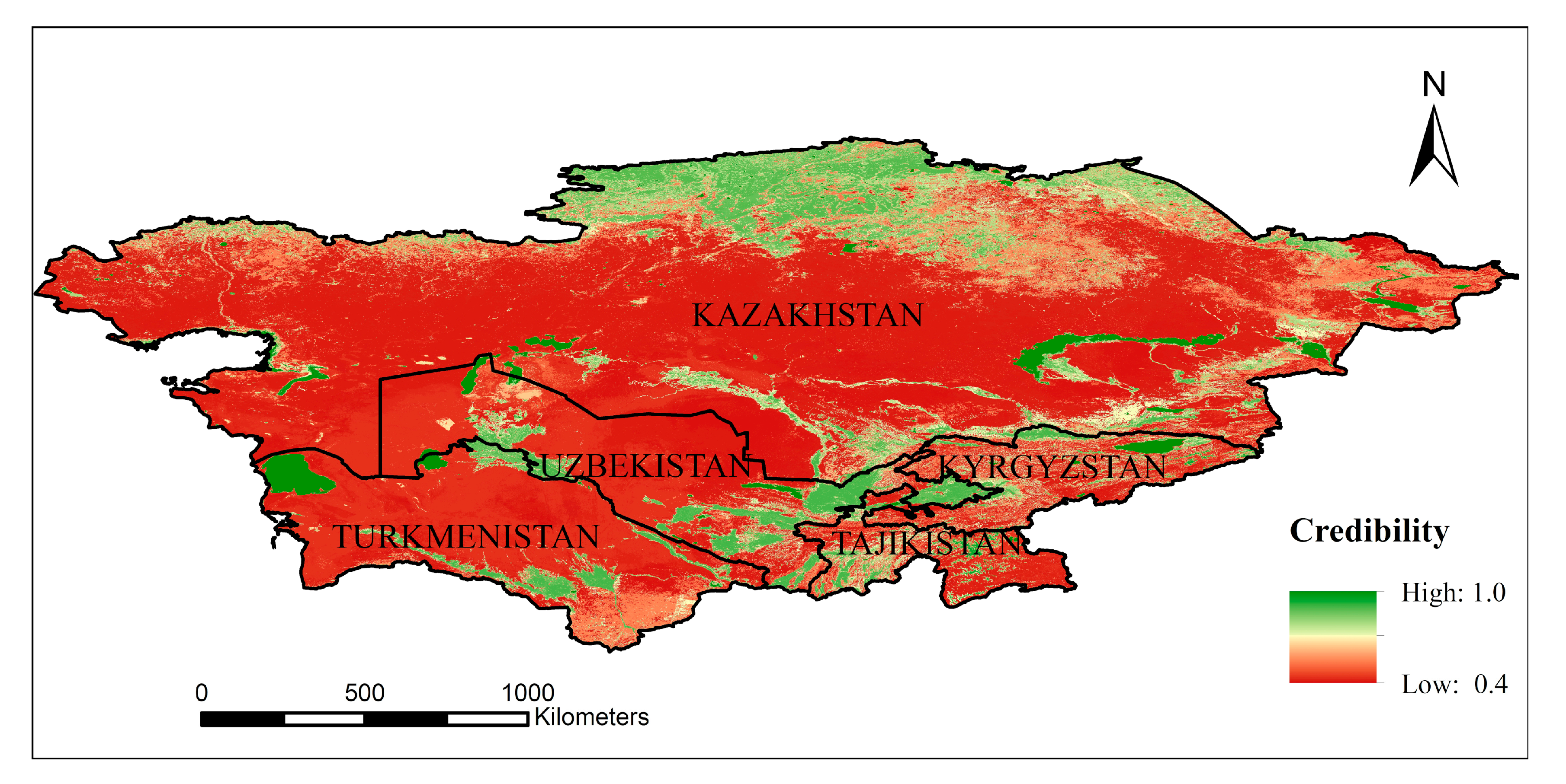
We considered the credibility of evidence, which refers to the degree of support for each target category and improved it on the basis of the Dempster-Shafer evidence synthesis rule (Figure 4). Assuming that the basic probability functions corresponding to n products were m1, m2, …, mn, and the subsets in each function were A1, A2, …, An, the evidence synthesis could be conducted by the following formula [50]:
m ( A ) = ( 1 K ) A 1 A 2 A n = A m 1 ( A 1 ) m 2 ( A 2 ) m n ( A n ) 1 K + K ε 1 n i = 1 n m i ( A )
K = A i B j = m 1 ( A i ) m 2 ( B j )
ε = e k
k = 1 n ( n 1 ) / 2 i < j A i B j = m i ( A i ) m j ( B j )
where m(A) is the composite probability of category A; K reflects the degree of conflict of the overall evidence; ε represents the credibility of the evidence, and k is the mean value of the sum of the conflicts of each pair of evidence items in n pieces of evidence. Finally, the fusion result was obtained according to the principle of maximum trust.

2.3.4. Data Comparison and Accuracy Verification

Accuracy Verification

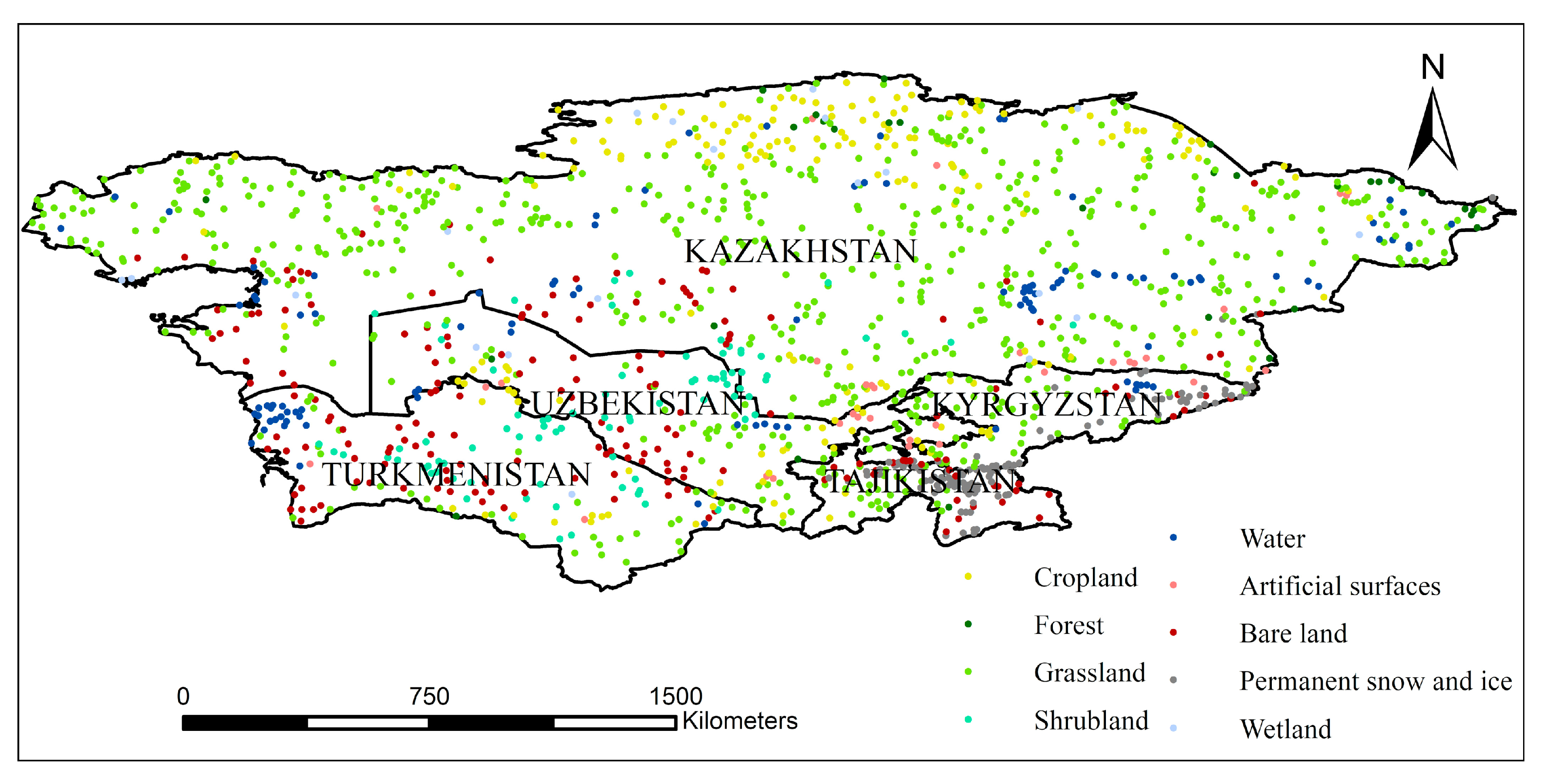
A set of verification plots was produced for the accuracy evaluation and comparison of multi-source landcover products and fusion correction results. A random sampling method was adopted, and supplementary sampling was conducted for landcovers that accounted for a small proportion of the total area. According to the data resolution of the landcover products, a sample area of 300 × 300 m was randomly arranged in the study area (Figure 5). We used the high-resolution images in Google Earth for 2015 to determine the type of features in the plot. The high-resolution remote sensing images in Google earth are mostly high-definition images from Worldview satellites, with a spatial resolution of 0.3~0.5 m. If high-resolution images for 2015 were not available, a high-resolution image of the time phase closest to 2015 was selected. There were 1437 plots in total, including 187 cropland plots, 30 forest plots, 675 grassland plots, 84 shrubland plots, 107 water plots, 33 plots containing artificial surfaces, 183 plots containing bare land, 118 plots containing permanent snow and ice, and 20 wetland plots.
We adopted an accuracy verification method derived from a confusion matrix. The overall accuracy (OA), producer accuracy (PA), user accuracy (UA), and kappa coefficient were used to measure the accuracy and consistency of the fusion results. The calculation formula was as follows [1,6,12]:
OA = i = 1 9 n i i N × 100 %
PA = n i i n + i × 100 %
UA = n i i n i + × 100 %
Kappa = OA P e 1 P e
P e = i = 1 n n + i n i + N 2
where N is the total number of verification samples; i is the ith landcover type; nii is the number of correctly classified samples; n+i is the plot number of type i in the reference data, and ni+ is the number of plots of type i in the verification data; Pe is the proportion of misinterpretation caused by accidental factors.

Similarity Analysis of Land Cover Type Area

A landcover type area similarity analysis was applied to compare the differences between products, fusion results, and landcover statistics. This cannot only quantitatively analyze the degree of similarity between the two types of landcover data but also quantitatively describe the difference between landcover data and statistics for a certain landcover type. The coefficient of determination R2 can reflect the degree of fit between the land area of each country calculated by the landcover products and the statistical landcover area. The greater the value, the higher the degree of fit [18]. The root-mean-square error (RMSE) can reflect the difference between the estimated landcover area from the products and the statistics [18]. For the analysis of the similarity between landcover products and statistics for a certain landcover type, the correlation coefficient R was used for evaluation. The larger the R, the more significant the correlation [18].
R = k = 1 n ( x k i x ¯ ) ( y k i y ¯ ) k = 1 n ( x k i x ¯ ) 2 k = 1 n ( y k i y ¯ ) 2
RMSE = k = 1 N ( x k i y k i ) 2 N
where xk is the area of ith landcover type in the kth country determined by a landcover product, yk is the area of ith landcover type in the kth country determined by landcover statistics; x ¯ and y ¯ are the average areas of various landcover types in each country (km2) determined by the landcover product and statistics, and n is the number of items involved in the calculation.

2.3.5. Confusion Analysis

Confusion analysis is to observe whether there is a mixture of other landcover types for the specific landcover type and analyze the degree of confusion. It used the verification sample to verify the classification accuracy of the fusion result, recorded the landcover types of the fusion result corresponding to each verification sample, and calculate the degree of consistency between each category and the verification sample by category. Then, we can record and calculate the ratio of misclassified land type number to the total number. The degree of confusion can indicate the accuracy of the classification of each area and its confusion with other landcover types in order to conduct a more detailed accuracy analysis of the fused landcover product.

3. Results and Analysis

3.1. Accuracy Verification Based on High-Resolution Image Plots

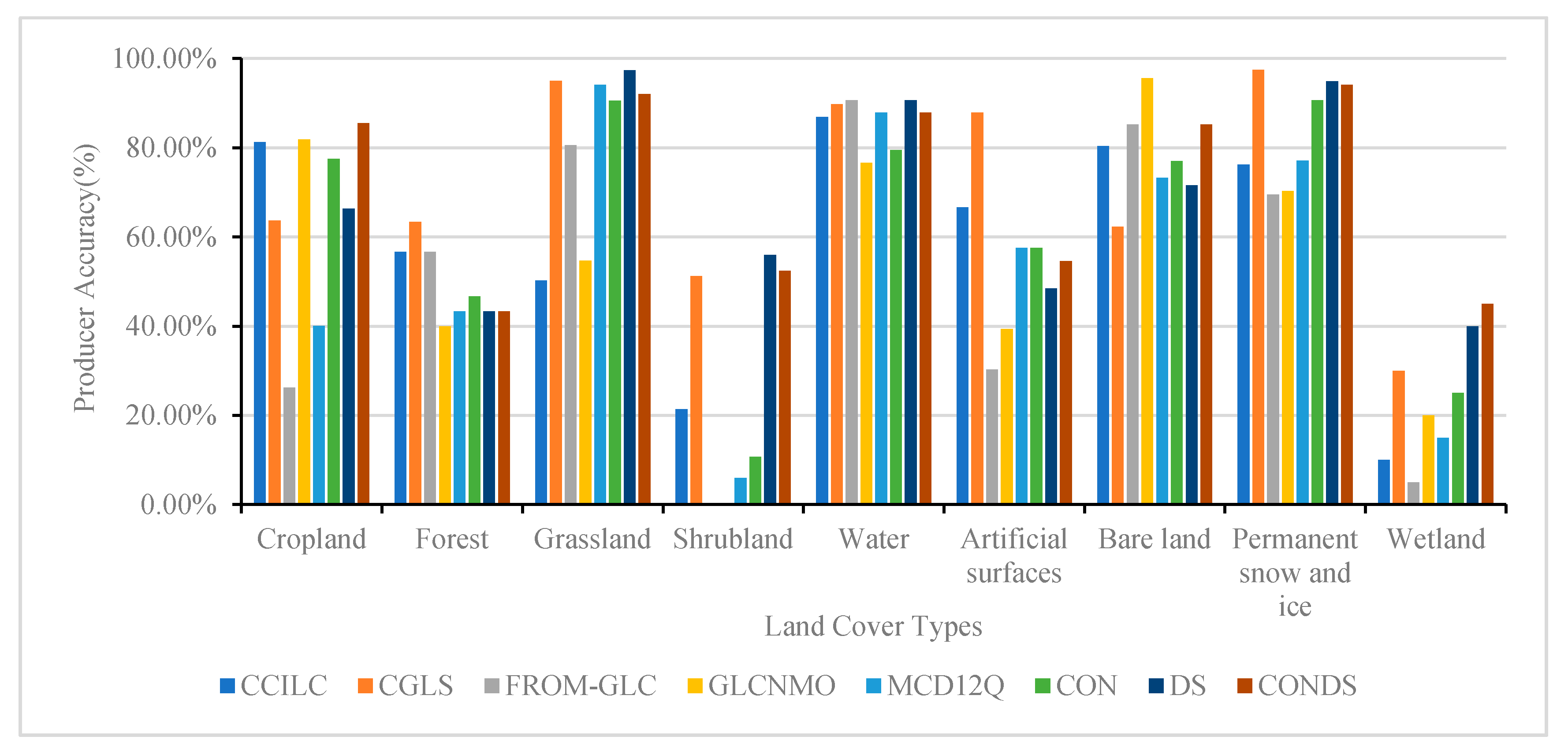
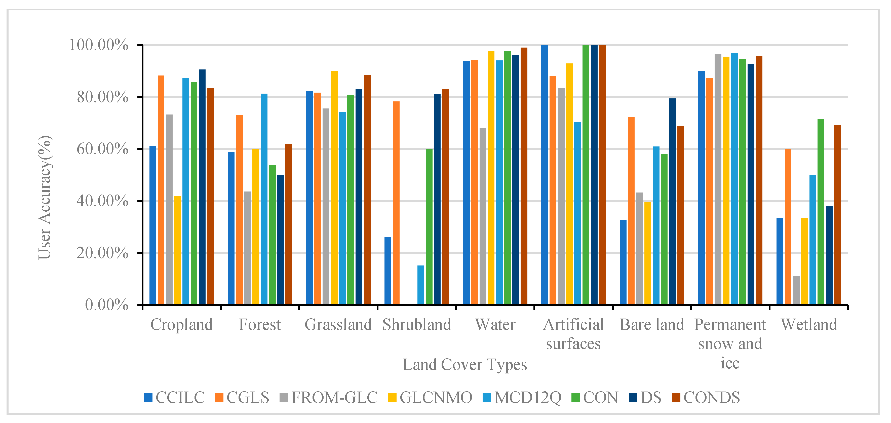
The accuracy of the five existing landcover comprehensive products and the three fusion products generated in this study (we define: the fusion result using only spatial consistency analysis is CON, the fusion result using only Dempster-Shafer evidence theory is DS, and the fusion result using the combination of the two methods is CONDS.) was verified, and the OA, PA, and UA of each product and the fusion results were obtained. Among the various products, the OA was highest for CGLS, reaching 76.27%, and the OA of the fusion result was higher than that of each product (Table 4). There was an obvious improvement in accuracy following the fusion based on spatial consistency and Dempster-Shafer evidence theory, and the consistency with the real surface was higher than for any product, with an overall accuracy of 85.32%. In the PA verification, shrubland and wetland had the lowest values, and the fusion result increased the PA of these two landcovers by 36.67–40.24% and 9–29%, respectively (Figure 6). The UA of each product and the fusion result were generally high, although the values for bare land and wetland were low, with average accuracies of 49.67% and 37.56%, respectively. The fusion result indicated an increase in accuracy by 8.35–29.72% and 0.54–33.87%, respectively. Except for artificial surfaces and forest, the PA values following the fusion were significantly lower than the results obtained for CGLS, while the accuracy was improved to varying degrees for the other landcover types (Figure 7). The accuracy of the various landcover products for forest land was not high, except for CGLS. When performing a spatial consistency analysis, it is easy to overlook the presence of forests using the various products, and therefore, the accuracy for forest land was low.

3.2. Accuracy Verification Based on Land Cover Statistics

We calculated and compared the RMSE, R2, and correlation coefficient R of the landcover areas obtained from the five comprehensive products and the fusion results obtained using the landcover statistics. The relationship between the land area of each product, the fusion results, and the landcover statistics is shown in Figure 8. It can be seen that the fusion result based on spatial consistency discrimination had the highest consistency with the landcover statistics, with an R2 value of 0.99 and the lowest RMSE. The results based on the fusion of the two methods were consistent with the 1:1 line. Among the five products, CGLS and FROM-GLC had the best-fitting relationship with the 1:1 line, which may be due to their higher spatial resolution. The CCI-LC results deviated greatly from the 1:1 line, which was related to the existence of mixtures of landcover types in its definition system, and indicated that the product significantly underestimated the area of certain landcover types. When the similarities among areas of certain landcover types were calculated, each product was found to have a high similarity for cropland, forest, and grassland but a low similarity for water. The fusion process could effectively improve the categorization of water (Table 5).

3.3. Analysis of Land Cover Characteristics in Central Asia

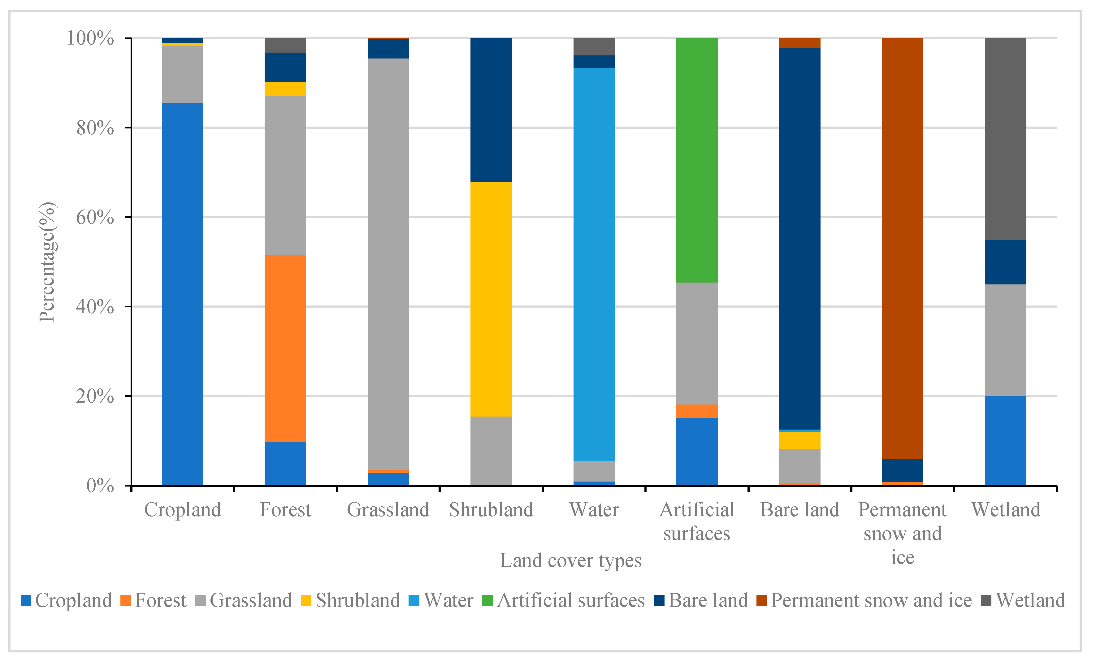
The analysis method based on the combination of spatial consistency discrimination and the improved Dempster-Shafer evidence theory combines the advantages of each method and takes into account the expression of spatial consistency and statistical consistency, and therefore the results produced were selected as the final fusion results. A confusion analysis of the landcover types revealed that each category had different degrees of confusion with other categories. Forest and grassland, and shrubland and bare land had the highest degrees of confusion, reaching 36.67% and 32.14%, respectively. Wetland had the next highest degree of confusion, which was mainly manifested through the wrong classification of cropland, grassland, and bare land. The appearance of artificial surfaces was confused with cropland, forest, and grassland, with the reason for the confusion being a misclassification due to the abundant green landscape in the city. Permanent snow and ice can be confused with bare land, and it may be considered to be bare ground when the snow melts to expose the surface (Figure 9).
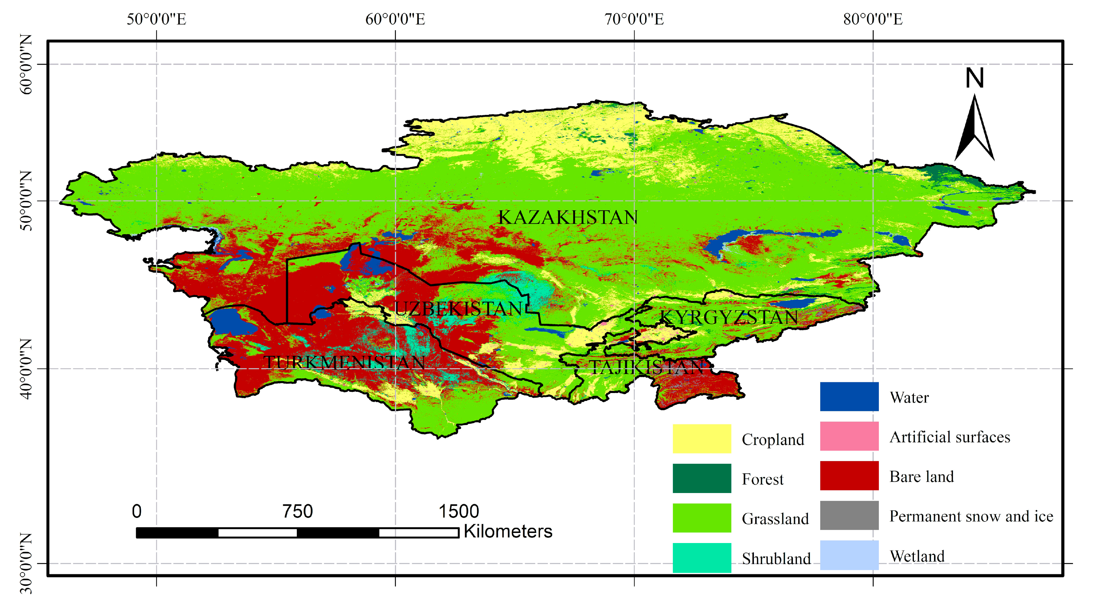
The main landcover types of the five Central Asian countries were grassland (58.17%) and bare land (22.31%), followed by cropland (12.08%), water (2.74%), shrubland (2.68%), forest (1.05%), permanent snow and ice (0.41%), and wetland (0.37%), while artificial surfaces accounted for the lowest proportion of landcover (Figure 10). Grassland was mainly distributed in central and southeastern Kazakhstan, which accounted for about 80% of the total grassland area. The remaining 20% of grassland was more evenly distributed in eastern Uzbekistan, western Kyrgyzstan, western Tajikistan, and northern Turkmenistan. About 90% of the bare land was distributed in the southwestern part of the region, namely southwestern Kazakhstan, western Uzbekistan, and northern Turkmenistan. The bare land was mainly desert, with the Karakum Desert in Turkmenistan being the largest desert in the region. Shrublands were often distributed around bare land, with most shrubs growing in desert areas along river basins and other locations. Cropland was mainly distributed at higher latitudes in the northern plains of Kazakhstan, which accounted for 75.39% of the total cropland area. Other countries had lesser amounts of loosely distributed cropland. The water bodies of the five Central Asian countries were mainly inland lakes, including Karabogazgor Bay in Turkmenistan, Sarygamysh Lake on the border of Turkmenistan and Uzbekistan, the Aral Sea on the border of Uzbekistan and Kazakhstan, Balkhash Lake in Kazakhstan, and Issyk-Kul Lake in Kyrgyzstan. The area of permanent snow and ice was mostly distributed in the Pamirs and Tianshan Mountains on the border between central Tajikistan and the eastern part of Kyrgyzstan, which is an area of high altitude. Around 80% of the forest land was concentrated in the Altai Mountains on the eastern border of Kazakhstan.

4. Discussion

Based on an analysis of spatial consistency and the improved Dempster-Shafer evidence theory, we integrated the results obtained from various landcover products for the five countries in Central Asia. The results proved that a data fusion could improve the data accuracy to varying degrees. An accuracy evaluation of the landcover data revealed that the accuracy improvement (from large to small) of the various methods followed the order of the combination of two methods > improved Dempster-Shafer evidence theory > spatial consistency discrimination. Compared with the other two methods, the accuracy of the combined method increased by 1.46% and 6.32%, respectively, and the similarity between the area of each category and landcover statistics was improved when compared with the use of the improved Dempster-Shafer evidence theory. According to previous studies, the results obtained using spatial consistency discrimination can be compared with FAO statistics during the fusion process, resulting in an improvement in the accuracy of landcover type determination. However, due to the varying qualities of the different landcover products, their accuracy was significantly affected in areas with a low consistency of multi-source products, i.e., the method was not sensitive to areas with high spatial location uncertainty [16,18]. The improved Dempster-Shafer evidence theory could better manage this spatial position uncertainty. For regions with low spatial consistency, the fusion result was more consistent with the real surface, and the accuracy was improved [22,23]. The combination of the two methods could comprehensively consider landcover statistics and spatial information, and therefore the fusion results not only improved the accuracy of plot evaluation but also matched the landcover statistics.
The method proposed in this study based on the combination of spatial consistency discrimination and Dempster-Shafer evidence theory could effectively integrate and modify the existing multi-source landcover products to produce high-precision landcover data. Taking the FAO landcover statistics as a baseline, regions with a higher spatial consistency were extracted, which ensured that the extracted regions had high spatial accuracy and statistical consistency [17,18]. The improved Dempster-Shafer evidence theory could effectively deal with the uncertainty of low-consistency areas. The Dempster-Shafer evidence theory has been used to integrate landcover products in previous studies, but in studies where there was a high degree of conflict in the evidence, paradoxes were prone to appear [24,50]. Considering that the landcover in Central Asia is dominated by grassland, of which desert grassland is the main component [51], the difficulty of distinguishing between bare land and grassland may lead to such conflicts of evidence. Therefore, we introduced the concept of credibility and improved the Dempster-Shafer evidence theory to avoid abnormal results caused by these conflicts of evidence.
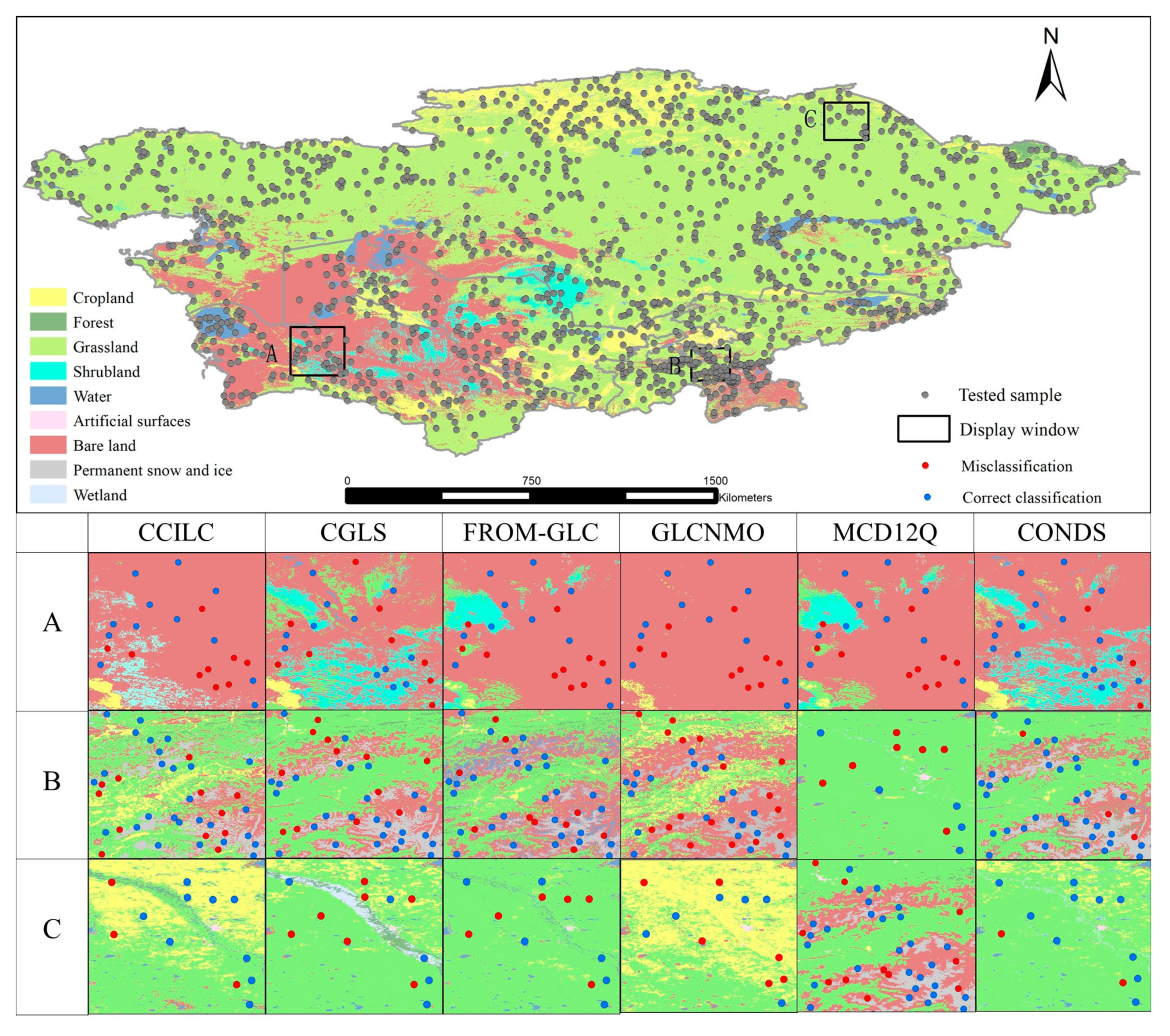
The accuracy assessment based on high-resolution plots showed that the OA of the existing landcover products in the five Central Asian countries was 60% to 80%. The accuracy of the products used in the study is generally not high [32], with only CGLS reaching more than 75%. Accurate unification and redefinition of classification systems before fusion can reduce the impact of any differences in classification systems on data consistency [12,15,22]. The accuracy of the input data is also one of the factors that affect the fusion of multi-source landcover data [52,53]. If there is a certain type of landcover and only one of the input products has high accuracy, the high-precision products will be ignored, resulting in low accuracy of the fusion results. This issue needs to be considered in future research, single-type landcover products have higher accuracy, and the differences in the accuracy of each product category in a comprehensive product can complement each other in the integration process. Although CCI-LC and GLCNMO had the lowest OA, they had the highest PA for cropland. CGLS had the highest OA, while the PA for cropland and bare land were lower than the values of the other products. The forest category accuracy for most products was low, although the accuracy of the PALSAR product was high. The difference between PA and UA reflects the accuracy of the product’s estimation of landcover type [54]. The PA of cropland in FROM-GLC is very low (26.2%), while its UA is very high (73.13%), which shows that this product over-underestimates the area of cropland. Because the interpretation of shrubland, wetland and artificial surfaces are easy to be confused with other categories, their PA and UA are also quite different. Among them, the PA-UA difference of shrubland is 27%, the PA-UA difference of wetland is 30%~35%, and the difference in PA-UA of artificial surfaces is 53%. It shows that each product also has a relatively obvious underestimation of shrubland, wetland and artificial surfaces. At the same time, in the accurate evaluation of each category, the importance of user accuracy should also be emphasized. Both CCI-LC and GLCNMO had a low user accuracy for cropland, indicating that they overestimated the cropland area to a certain extent, while CGLS underestimated the cropland area. The results of this study integrated the high-precision categories of landcover products, and compared the results with the input data, improving the accuracy in areas with high landscape heterogeneity (Figure 11). Wetland is the most difficult landcover type to map worldwide, but the ecosystem services provided to human society by wetlands have the greatest monetary value [55,56]. The accuracy of the fusion result for wetland was significantly improved, and the ability to map wetland has therefore been improved. Compared with the input data, the PA and UA of each category of the fusion result were more consistent, which effectively compensated for the overestimation of the input data.
The degree of confusion between forest, bare land, and grassland is relatively high. This may be because landcover changes in Central Asia have accelerated since the disintegration of the Soviet Union and have mainly been manifested in the transfer of forest to grassland, grassland to cropland, and bare land to forest and grassland [29,57]. The accuracy of the shrubland area in terms of the input data and fusion result was very low, which could be due to the fact that shrubs are easily confused with bare land and grass. Shrubland is a landcover type that transitions from grassland to bare land (land desertification) or from bare land to grassland (desert shrub). To a certain extent, the spectral characteristics and phenological characteristics of shrubland, grassland, and bare land are very similar [58]. There was also a certain degree of confusion between wetland, cropland, and grassland. Therefore, the ability to distinguish shrublands and wetlands as well as the ability to distinguish between shrublands and bare lands, wetlands and croplands, grasslands needs to be improved in future landcover products.
Compared with ground surveys, the use of high-resolution images stored in Google Earth as reference data to evaluate the accuracy of products and datasets is not limited to the current time period, and it takes much less time to conduct. Thus, these images have become widely used in studies, and their scientific validity can be guaranteed. There are limitations in comparing input data and fusion results with statistics. First, the statistics obtained from the FAO statistical database are national-level statistical data, while sub-national data are difficult to obtain. Second, the quality of statistical data is affected by human factors and may be insufficient for use. These are factors that could affect the comparison of data sets with statistics [59,60]. Liu et al. proposed the use of planetary boundary theory and net primary productivity (NPP) data to correct statistics, improving the calculation method of human appropriation of net primary production (HANPP), and combined MODIS NPP products with observations and models of physical factors that restrict crop growth to explore the prevalence of data misreporting, which may provide a method for the accuracy of statistical data [61].
Although the spatial resolution of landcover products is constantly improving, data fusion is still recognized as an effective method to improve the quality of landcover information. Considering the problems of existing fusion methods, improvements should be made in several areas in the future. First, when unifying the spatial resolution, attention should be given to the matching of plot size and product resolution, and appropriate upscaling and downscaling methods should be adopted to reduce information loss. Second, statistical data can be corrected in certain areas using data such as NPP and night light remote sensing to avoid false positives during a census. Finally, each fusion method has its own advantages and disadvantages, and the combined use of multiple methods is, therefore, the development direction of multi-source land data fusion. The spatial consistency discrimination technology and the improved Dempster-Shafer theory used in this paper also have some limitations. The application of this method is limited to existing data sets with similar release time. For other applications such as the production of landcover products, the method remains to be improved.

5. Conclusions

In this study, we selected the five countries in Central Asia as the research area, integrated multi-source landcover products, introduced spatial consistency discrimination and the improved Dempster-Shafer evidence theory, set landcover statistical data as the baseline conditions, and designed landcover product amendment rules and technical processes to establish a multi-source landcover fusion and correction method. This was based on the integration of CCI-LC, CGLS, FROM-GLC, GLCNMO, MCD12Q, GFSAD30, PALSAR, GSWD, and GHS-BUILT to obtain 300 m resolution landcover data and verify the accuracy and landcover statistics. The method of spatial consistency discrimination had the best agreement with statistical data, with an R2 value of 0.99. The improved Dempster-Shafer evidence theory fusion method had several advantages in location determination and accuracy improvement, with the accuracy, increased by 4.86% compared to the method of spatial consistency discrimination. The kappa coefficient increased by 0.07. The fusion method proposed in this study used Dempster-Shafer evidence theory to resolve the uncertainty of low consistency areas based on spatial consistency discrimination technology and also resolved the paradox problem that exists in the Dempster-Shafer evidence theory. The OA of the fusion result was 85.32%, which was higher than that of the individual products used in Central Asia, with an average increase of 16.04, and kappa coefficient of 0.80, The consistency with the real surface was better than that of the individual products, and the consistency of the statistical data and spatial consistency were taken into account. The fusion process was, therefore, shown to be effective. Cropland, grassland, water, bare land, and permanent snow and ice all had a high PA of above 80%. Except for forest, bare land, and wetland, the UA also reached 80% for the different landcover categories. The fusion method developed in this study can be used for the fusion of multi-source data. The combination of multiple methods is the development direction of multi-source landcover data fusion.

Author Contributions

Conceptualization, K.L. and E.X.; methodology, K.L. and E.X.; validation, K.L.; formal analysis, K.L.; resources, E.X.; writing—original draft preparation, K.L.; writing—review and editing, E.X.; supervision, E.X.; project administration, E.X.; funding acquisition, E.X. All authors have read and agreed to the published version of the manuscript.

Funding

This research was funded by the Strategic Priority Research Program of the Chinese Academy of Sciences (XDA20040201) and the National Natural Science Foundation of China (41671097).

Institutional Review Board Statement

Not applicable.

Informed Consent Statement

Not applicable.

Data Availability Statement

This study was performed based on public-access data. The data that support the findings of this study are available from the corresponding author upon reasonable request.

Conflicts of Interest

The authors declare no conflict of interest.

References

  1. Yang, Y.; Xiao, P.; Feng, X.; Li, H.; Chang, X.; Feng, W. Comparison and assessment of large-scale land cover datasets in China and adjacent regions. J. Remote Sens. 2014, 18, 453–475. (In Chinese) [Google Scholar] [CrossRef]
  2. Zubaida, M.; Xia, J.; Polat, M.; Zhang, R. Land use and landscape pattern changes in the middle reaches of the Keriya River. Acta Ecol. Sin. 2019, 39, 2322–2330. (In Chinese) [Google Scholar]
  3. Suess, S.; Linden, S.; Okujeni, A.; Griffiths, P.; Schwieder, M.; Hostert, P. Characterizing 32 years of shrub cover dynamics in southern Portugal using annual Landsat composites and machine learning regression modeling. Remote Sens. Environ. 2018, 219, 353–364. [Google Scholar] [CrossRef]
  4. Lees, K.J.; Quaife, T.; Artz, R.R.E.; Khomik, M.; Clark, J.M. Potential for using remote sensing to estimate carbon fluxes across northern peatlands—A review. Sci. Total Environ. 2018, 615, 857–874. [Google Scholar] [CrossRef] [PubMed]
  5. Hu, Y.; Zhang, Q.; Dai, Z.; Huang, M.; Yan, H. Agreement analysis of multi-sensor satellite remote sensing derived land cover products in the Europe Continent. Geogr. Res. 2015, 34, 1839–1852. (In Chinese) [Google Scholar]
  6. Grekousis, G.; Mountrakis, G.; Kavouras, M. An overview of 21 global and 43 regional land-cover mapping products. Int. J. Remote Sens. 2015, 36, 5309–5335. [Google Scholar] [CrossRef]
  7. Lai, C.; Yan, M.; Du, W.; Hu, Y. The Variations and Causes of Grassland Distribution in Kazakhstan from the Global Land Cover Datasets. J. Geo-Inf. Sci. 2019, 21, 372–383. (In Chinese) [Google Scholar]
  8. Hou, W.; Hou, X. Data Fusion and Accuracy Analysis of Multi-Source Land Use/Land Cover Datasets along Coastal Areas of the Maritime Silk Road. Int. J. Geo-Inf. 2019, 8, 557. [Google Scholar] [CrossRef] [Green Version]
  9. Yadav, K.; Congaltion, R.G. Accuracy Assessment of Global Food Security-Support Analysis Data (GFSAD) Cropland Extent Maps Produced at Three Different Spatial Resolutions. Remote Sens. 2018, 10, 1800. [Google Scholar] [CrossRef] [Green Version]
  10. Lapini, A.; Pettinato, S.; Santi, E.; Paloscia, S.; Fontanelli, G.; Garzelli, A. Comparison of Machine Learning Methods Applied to SAR Images for Forest Classification in Mediterranean Areas. Remote Sens. 2020, 12, 369. [Google Scholar] [CrossRef] [Green Version]
  11. Xu, Z.; Luo, Q.; Xu, Z. Consistency of Land Cover Data Derived from Remote Sensing in Xinjiang. J. Geo-Inf. Sc. 2019, 21, 427–436. (In Chinese) [Google Scholar]
  12. Dai, Z.; Hu, Y.; Zhang, Q. Agreement Analysis of Multi-source Land Cover Products Derived from Remote Sensing in South America. Remote Sens. Inf. 2017, 32, 137–148. (In Chinese) [Google Scholar]
  13. Kuenzer, C.; Leinenkugel, P.; Vollmuth, M.; Dech, S. Comparing global land-cover products—Implications for geoscience applications: An investigation for the trans-boundary Mekong Basin. Int. J. Remote Sens. 2014, 35, 2752–2779. [Google Scholar] [CrossRef] [Green Version]
  14. Jung, M.; Henkel, K.; Herold, M.; Churkina, G. Exploiting synergies of global land cover products for carbon cycle modeling. Remote Sens. Environ. 2006, 101, 534–553. [Google Scholar] [CrossRef]
  15. Bai, Y.; Feng, M. Data fusion and accuracy evaluation of multi-source global land cover datasets. Acta Geogr. Sin. 2018, 73, 2223–2235. (In Chinese) [Google Scholar]
  16. Fritz, S.; You, L.; Bun, A.; See, L.; McCallum, I.; Schill, C.; Perger, C.; Liu, J.; Hansen, M.; Obersteiner, M. Cropland for sub-Saharan Africa: A synergistic approach using five land cover data sets. Geophys. Res. Lett. 2011, 38, 155–170. [Google Scholar] [CrossRef] [Green Version]
  17. Dmitry, S.; Ian, M.; Anatoly, S.; Steffen, F.; Florian, K.; Michael, O. A new hybrid land cover dataset for Russia: A methodology for integrating statistics, remote sensing and in situ information. J. Land Use Sci. 2011, 6, 245–259. [Google Scholar]
  18. Lu, M.; Wu, W.; You, L.; Chen, D.; Zhang, L.; Yang, P.; Tang, H. A Synergy Cropland of China by Fusing Multiple Existing Maps and Statistics. Sensors 2017, 17, 1613. [Google Scholar] [CrossRef] [Green Version]
  19. Dempster, A.P. Upper and Lower Probabilities Induced by a Multivalued Mapping. Ann. Math. Stat. 1967, 38, 325–339. [Google Scholar] [CrossRef]
  20. Shafer, G.A. A Mathematical Theory of Evidence. Technometrics 1978, 20, 106. [Google Scholar]
  21. Luo, Z.; Deng, Y. A Matrix Method of Basic Belief Assignment’s Negation in Dempster-Shafer Theory. IEEE Trans. Fuzzy Syst. 2020, 28, 2270–2276. [Google Scholar] [CrossRef]
  22. Ran, Y.; Li, X.; Lu, L. China Land Cover Classification at 1 km Spatial Resolution Based on a Multi-source Data Fusion Approach. Adv. Earth Sci. 2009, 24, 192–203. (In Chinese) [Google Scholar]
  23. Song, H.; Zhang, X. Precision analysis and validation of multi-sources landcover products derived from remote sensing in China. Trans. Chin. Soc. Agric. Eng. 2012, 28, 207–214. (In Chinese) [Google Scholar]
  24. Zadeh, L.A. Fuzzy Sets and Their Application to Pattern Classification and Clustering Analysis. Classif. Clust. 1977, 251–299. [Google Scholar]
  25. Luo, H.; Liu, C.; Wu, C.; Guo, X. Urban Change Detection Based on Dempster-Shafer Theory for Multitemporal Very High-Resolution Imagery. Remote Sens. 2018, 10, 980. [Google Scholar] [CrossRef] [Green Version]
  26. Koksalmis, E.; Kabak, Ö. Sensor fusion based on Dempster-Shafer theory of evidence using a large scale group decision making approach. Int. J. Intell. Syst. 2020, 35, 1126–1162. [Google Scholar] [CrossRef]
  27. Chen, X.; Bai, J.; Li, X.; Luo, G.; Li, J.; Li, B. Changes in land use/land cover and ecosystem services in Central Asia during 1990-2009. Curr. Opin. Environ. Sustain. 2013, 5, 116–127. [Google Scholar] [CrossRef]
  28. Lioubimtseva, E.; Cole, R.; Adams, J.M.; Kapustin, G. Impacts of climate and land-cover changes in arid lands of Central Asia. J. Arid Environ. 2005, 62, 300–308. [Google Scholar] [CrossRef]
  29. Fan, Z.; Li, S. Change pattern of land cover and its driving force since 2001 in the New Eurasian Continental Bridge Economic Corridor. Acta Ecol. Sin. 2019, 39, 5015–5027. (In Chinese) [Google Scholar]
  30. Li, J.; Chen, H.; Zhang, C.; Pan, T. Variations in ecosystem service value in response to land use/land cover changes in Central Asia from 1995–2035. Peerj 2019, 7, 7665–7686. [Google Scholar] [CrossRef]
  31. De Beurs, K.M.; Henebry, G.M.; Owsley, B.C.; Sokolik, I. Using multiple remote sensing perspectives to identify and attribute land surface dynamics in Central Asia 2001–2013. Remote Sens. Environ. 2015, 170, 48–61. [Google Scholar] [CrossRef]
  32. Sun, B.; Chen, X.; Zhou, Q. Uncertainty Assessment of GLOBELAND30 Land Cover Data Set over Central Asia. Int. Arch. Photogramm. Remote Sens. Spat. Inf. Sci. 2016, XLI-B8, 1313–1317. [Google Scholar] [CrossRef]
  33. Han, Q.; Luo, G.; Bai, J.; Li, J.; Li, C.; Fan, B.; Wang, Y. Characteristics of land use and cover change in Central Asia in recent 30 years. Arid Land Geogr. 2012, 35, 909–918. (In Chinese) [Google Scholar]
  34. Perez-Hoyos, A.; Rembold, F.; Kerdiles, H.; Gallego, J. Comparison of Global Land Cover Datasets for Cropland Monitoring. Remote Sens. 2017, 9, 1118. [Google Scholar] [CrossRef] [Green Version]
  35. Song, R.; Muller, J.; Kharbouche, S.; Woodgate, W. Intercomparison of Surface Albedo Retrievals from MISR, MODIS, CGLS Using Tower and Upscaled Tower Measurements. Remote Sens. 2019, 11, 644. [Google Scholar] [CrossRef] [Green Version]
  36. Xu, Y.; Yu, L.; Feng, D.; Peng, D.; Li, C.; Huang, X.; Lu, H.; Gong, P. Comparisons of three recent moderate resolution African land cover datasets: CGLS-LC100, ESA-S2-LC20, and FROM-GLC-Africa30. Int. J. Remote Sens. 2019, 40, 6185–6202. [Google Scholar] [CrossRef]
  37. Jean-Francois, P.; Andrew, C.; Noel, G.; Alan, S. High-resolution mapping of global surface water and its long-term changes. Nature 2016, 540, 418–422. [Google Scholar]
  38. Corbane, C.; Pesaresi, M.; Politis, P.; Syrris, V.; Florczyk, A.J.; Soille, P.; Maffenini, L.; Burger, A.; Vasilev, V.; Rodriguez, D.; et al. Big earth data analytics on Sentinel-1 and Landsat imagery in support to global human settlements mapping. Big Earth Data 2017, 1, 118–144. [Google Scholar] [CrossRef] [Green Version]
  39. Corbane, C.; Pesaresi, M.; Kemper, T.; Politis, P.; Florczyk, A.J.; Syrris, V.; Melchiorri, M.; Sabo, F.; Soille, P. Automated global delineation of human settlements from 40 years of Landsat satellite data archives. Big Earth Data 2019, 3, 140–169. [Google Scholar] [CrossRef]
  40. Gong, P.; Wang, J.; Yu, L.; Zhao, Y.; Zhao, Y.; Liang, L.; Niu, Z.; Huang, X.; Fu, H.; Liu, S.; et al. Finer resolution observation and monitoring of global land cover: First mapping results with Landsat TM and ETM+ data. Int. J. Remote Sens. 2013, 34, 2607–2654. [Google Scholar] [CrossRef] [Green Version]
  41. Yu, L.; Liu, X.; Zhao, Y.; Yu, C.; Gong, P. Difficult to map regions in 30 m global land cover mapping determined with a common validation dataset. Int. J. Remote Sens. 2018, 39, 4077–4087. [Google Scholar] [CrossRef]
  42. Tateishi, R.; Uriyangqai, B.; Al-bilbisi, H.; Ghar, M.A.; Tsend-Ayush, J.; Kobayashi, T.; Kasimu, A.; Hoan, N.T.; Shalaby, A.; Alsaaideh, B.; et al. Production of global land cover data—GLCNMO. Int. J. Digit. Earth 2011, 4, 22–49. [Google Scholar] [CrossRef]
  43. Alimujiang, K.; Tateishi, R. GLCNMO global urban mapping, validation and comparison with existing global urban maps. J. Remote Sens. Soc. Jpn. 2008, 28, 427–440. [Google Scholar]
  44. Hua, T.; Zhao, W.; Liu, Y.; Wang, S.; Yang, S. Spatial Consistency Assessments for Global Land-Cover Datasets: A Comparison among GLC2000, CCI LC, MCD12, GLOBCOVER and GLCNMO. Remote Sens. 2018, 10, 1846. [Google Scholar] [CrossRef] [Green Version]
  45. Liu, Q.; Zhang, Y.; Liu, L.; Li, L.; Qi, W. The spatial local accuracy of land cover datasets over the Qiangtang Plateau, High Asia. J. Geogr. Sci. 2019, 29, 1841–1858. [Google Scholar] [CrossRef] [Green Version]
  46. Sulla-Menashe, D.; Gray, J.M.; Abercrombie, S.P.; Friedl, M.A. Hierarchical mapping of annual global land cover 2001 to present: The MODIS Collection 6 Land Cover product. Remote Sens. Environ. 2019, 222, 183–194. [Google Scholar] [CrossRef]
  47. Shimada, M.; Itoh, T.; Motooka, T.; Watanabe, M.; Shiraishi, T.; Thapa, R.; Lucas, R. New global forest/non-forest maps from ALOS PALSAR data (2007–2010). Remote Sens. Environ. 2014, 155, 13–31. [Google Scholar] [CrossRef]
  48. Raucoules, D.; De Michele, M.; Aunay, B. Landslide displacement mapping based on ALOS-2/PALSAR-2 data using image correlation techniques and SAR interferometry. Application to Salazie Circle landslides (La Réunion Island). Geocarto Int. 2020, 35, 113–127. [Google Scholar] [CrossRef]
  49. Yu, L.; Wang, J.; Li, X.; Li, C.; Zhao, Y.; Gong, P. A multi-resolution global land cover dataset through multisource data aggregation. Sci. China Earth Sci. 2014, 57, 2317–2329. (In Chinese) [Google Scholar] [CrossRef]
  50. Sun, Q.; Ye, X.; Gu, W. A new combination rules of evidence theory. Acta Electron. Sin. 2000, 8, 117–119. (In Chinese) [Google Scholar]
  51. Zhang, X. Evaluation of Ecological Carrying Capacity in Central Asia and Mongolia Based on MODIS Satellite Data. Master’s Thesis, Beijing Jiaotong University, Beijing, China, 2018. [Google Scholar]
  52. Louise, L.; Audrey, J.; Bégué, A.; Danny, L.S.; Bernardin, Z. How Reliable is the MODIS Land Cover Product for Crop Mapping Sub-Saharan Agricultural Landscapes? Remote Sens. 2014, 6, 8541–8564. [Google Scholar] [CrossRef] [Green Version]
  53. Pérez-Hoyos, A.; García-Haro, F.J.; San-Miguel-Ayanz, J. A methodology to generate a synergetic land-cover map by fusion of different land-cover products. Int. J. Appl. Earth Obs. Geoinf. 2012, 19, 72–87. [Google Scholar] [CrossRef]
  54. Li, K.; Xu, E. Cropland data fusion and correction using spatial analysis techniques and the Google Earth Engine. GISci. Remote Sens. 2020, 57, 1026–1045. [Google Scholar] [CrossRef]
  55. Song, X.; Huang, C.; Townshend, J. Improving global land cover characterization through data fusion. Geo-Spat. Inf. Sci. 2017, 20, 141–150. [Google Scholar] [CrossRef] [Green Version]
  56. Costanza, R.; De Groot, R.; Sutton, P.; Van der Ploeg, S.; Anderson, S.J.; Kubiszewski, I.; Farber, S.; Turner, R.K. Changes in the Global Value of Ecosystem Services. Glob. Environ. Chang. 2014, 26, 152–158. [Google Scholar] [CrossRef]
  57. Ruan, H.; Yu, J. Changes in land cover and evapotranspiration in the five Central Asian countries from 1992 to 2015. Acta Geogr. Sin. 2019, 74, 1292–1304. [Google Scholar]
  58. Hu, Y.; Hu, Y. Land Cover Changes and Their Driving Mechanisms in Central Asia from 2001 to 2017 Supported by Google Earth Engine. Remote Sens. 2019, 11, 554. [Google Scholar] [CrossRef] [Green Version]
  59. Perez-Hoyos, A.; Udias, A.; Rembold, F. Integrating multiple land cover maps through a multi-criteria analysis to improve agricultural monitoring in Africa. Int. J. Appl. Earth Obs. Geoinf. 2020, 88, 102064. [Google Scholar] [CrossRef]
  60. Vancutsem, C.; Marinho, E.; Kayitakire, F.; See, L.; Fritz, S. Harmonizing and combining existing land cover/land use datasets for cropland area monitoring at the African continental scale. Remote Sens. 2013, 5, 19–41. [Google Scholar] [CrossRef] [Green Version]
  61. Liu, G.; Wang, X.; Baiocchi, G.; Casazza, M.; Meng, F.; Cai, Y.; Hao, Y.; Wu, F.; Yang, Z. On the accuracy of official Chinese crop production data: Evidence from biophysical indexes of net primary production. Proc. Natl. Acad. Sci. USA 2020, 117, 25434–25444. [Google Scholar] [CrossRef]
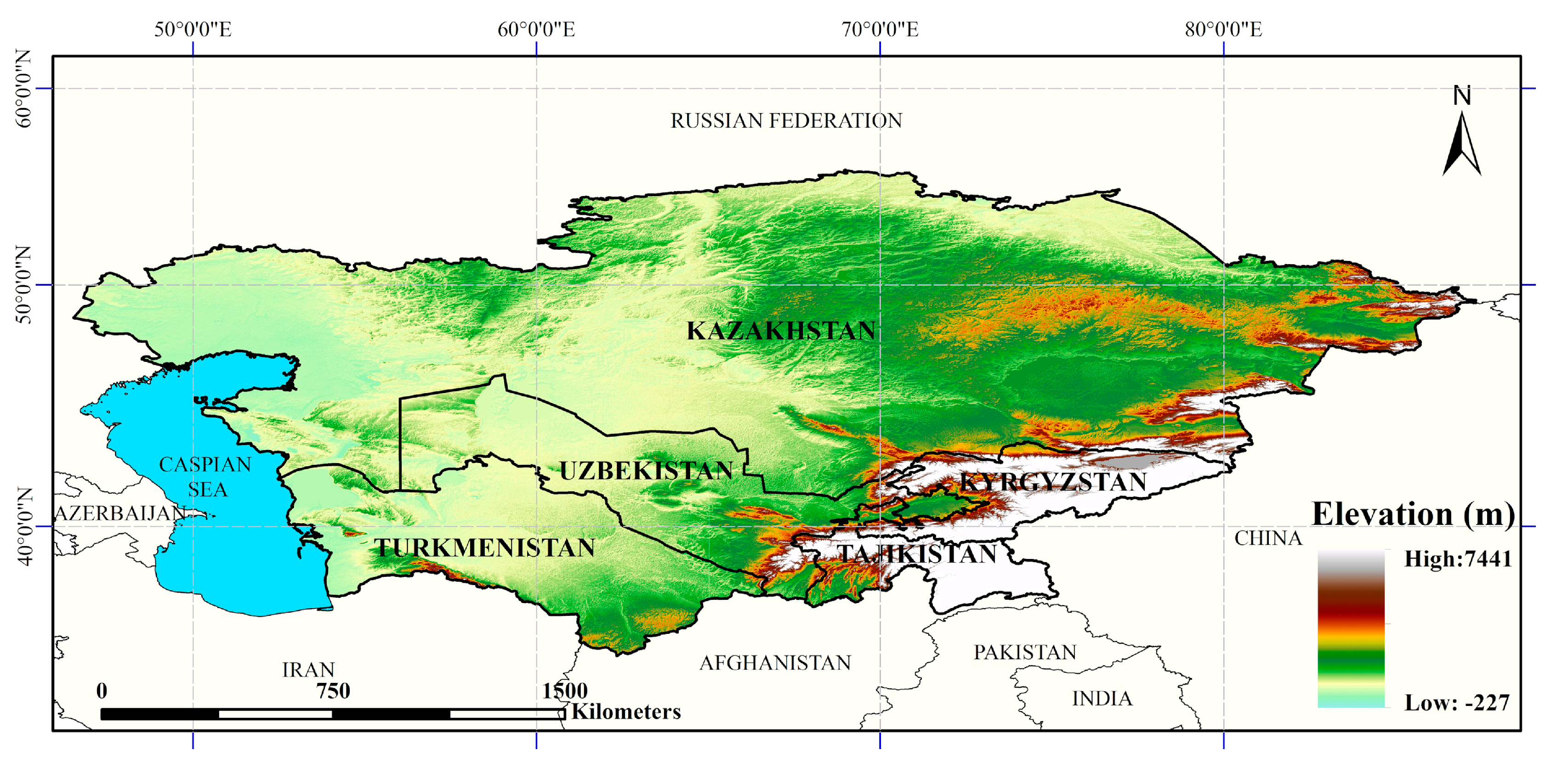
Figure 1. Overview map of the study area.
Remotesensing 13 00244 g001
Figure 2. Flow chart of multi-source landcover product integration and modification.
Remotesensing 13 00244 g002
Figure 3. Consistent spatial distribution of multiple landcover products: (a) cropland; (b) forest; (c) grassland; (d) shrubland; (e) water; (f) artificial surfaces; (g) bare land; (h) permanent snow and ice; (i) wetland.
Remotesensing 13 00244 g003aRemotesensing 13 00244 g003b
Figure 4. Improved Dempster-Shafer evidence theory: the distribution of credibility ε.
Remotesensing 13 00244 g004
Figure 5. The distribution map of validation samples for landcover/use data accuracy test.
Remotesensing 13 00244 g005
Figure 6. Producer accuracy of landcover products and fusion results.
Remotesensing 13 00244 g006
Figure 7. User accuracy of landcover products and fusion results.
Remotesensing 13 00244 g007
Figure 8. Correlation analysis and statistics of landcover products and fusion results and statistical data: (a) CCI-LC; (b) CGLS; (c) FROM-GLC; (d) GLCNMO; (e) MCD12Q; (f) CON; (g) DS; (h) CONDS.
Remotesensing 13 00244 g008
Figure 9. Multi-source landcover data fusion results in confusion of landcover types.
Remotesensing 13 00244 g009
Figure 10. Results of integration of multi-source landcover products in Central Asian study area.
Remotesensing 13 00244 g010
Figure 11. Spatial distribution of accuracy test for multiple landcover products and fusion results. (A) Karakum Desert; (B) Pamirs Plateau; (C) Turan Plain.
Remotesensing 13 00244 g011
Table 1. Basic information on nine landcover products.
ProductSourceSensorsClassification MethodResolution RatioOverall AccuracyClassification System
CCI-LCESAMERIS FR/RR SPOT-VGT AVHRR PROBA-VNeural networks300 m71.70%CCI-LC(37)
CGLSECJRCPROBA-VRandom forest100 m80.10%UN-LCCS(22)
FROM-GLCTsinghua University, ChinaTM ETM+Support vector machine, random forest30 m64.92%FROM-GLC(28)
GLCNMOISCGMMODISDecision tree500 m74.80%FAO-LCCS(20)
MCD12QBoston UniversityMODISDecision tree, neural network500 m71.60%IGBP(17)
GFSAD30USGSMODISMachine learning30 m94.80%
PALSARJAXAPALSARSupervised classification25 m94.81%
GSWDECJRCTM ETM+ OLISupervised classification30 m97.45%
GHS-BUILTECJRCTM ETM+ OLIMachine learning30 m83%
Table 2. Definition of landcover type in different landcover products.
CCI-LC [32]UN-LCCS [33,34]FAO-LCCS [40,41,42,43]IGBP [42,43,44]FROM-GLC [38,39]
Cropland10 Cropland, rainfed 20 Cropland, irrigated or post-flooding 30 Mosaic cropland (>50%)/natural vegetation (tree, shrub, herbaceous cover) (<50%)40 Cultivated and managed vegetation/agriculture (cropland)10 Cropland and paddy field 12 Cropland/other vegetation mosaic10 Croplands 13 Cropland/natural vegetation mosaics11 Rice paddy 12 Greenhouse 13 Other cropland 14 Orchard 15 Bare farmland
Forest50 Tree cover, broadleaved, evergreen, closed to open (>15%) 60 Tree cover, broadleaved, deciduous, closed to open (>15%) 70 Tree cover, needle-leaved, evergreen, closed to open (>15%) 80 Tree cover, needle-leaved, deciduous, closed to open (>15%) 90 Tree cover, mixed leaf type (broadleaved and needle-leaved) 100 Mosaic tree and shrub (>50%)/herbaceous cover (<50%)111 Closed (>70%) evergreen needle leaf 112 Closed to open (>70%) evergreen, broadleaf 113 Closed (>70%) deciduous needle leaf 114 Closed (>70%) deciduous broadleaf 115 Closed forest, mixed 116 Closed forest, unknown 121 Open (15–70%) evergreen needle leaf 122 Open (15–70%) evergreen broadleaf 123 Open (15–70%) deciduous needle-leaf 124 Open (15–70%) deciduous broadleaf 125 Open forest, mixed 126 Open forest, unknown20 Open (40–(20–10)%) trees (Woodland) 21 Broadleaved evergreen closed to open (>40%) trees 22 Broadleaved deciduous closed to open (>40%) trees 23 Needle-leaved evergreen closed to open (>40%) trees 24 Needle leaved deciduous closed to open (>40%) trees 25 Broadleaved/ needle-leaved closed to open trees20 Woody savannas 21 Evergreen broadleaf forests 22 Deciduous broadleaf forests 23 Evergreen needle-leaf forests 24 Deciduous needle-leaf forests 25 Mixed forests21 Broadleaf, leaf-on 22 Broadleaf, leaf-off 23 Needle-leaf, leaf-on 24 Needle-leaf, leaf-off 25 Mixed leaf, leaf-on 26 Mixed leaf, leaf-off
Grassland110 Mosaic herbaceous cover (>50%)/tree and shrub (<50%) 130 Grassland30 Herbaceous vegetation (tree and shrub coverage <10%)30 Closed to open herbaceous vegetation, single layer30 Grasslands31 Pasture 32 Natural grassland 33 Grassland, leaf-off
Shrubland120 Shrubland20 Shrubs (perennial woody plant without clear main stem, height <5 m)40 Closed to open shrubland (thicket)40 Closed/open shrublands, savannas41 Shrubland, leaf-on 42 Shrubland, leaf-off
Water210 Water bodies80 Permanent water bodies 200 Open sea50 Artificial/ natural waterbodies50 Water bodies60 Water
Artificial surfaces190 Urban areas50 Urban/built up60 Artificial surfaces and associated area(s)60 Urban and built-up lands80 Impervious surface
Bare land200 Bare areas 150 Sparse vegetation (tree, shrub, herbaceous cover) (<15%)60 Bare/sparse vegetation (tree coverage <10%)70 Herbaceous with sparse tree/shrub, sparse vegetation70 Barren sparse vegetation90 Bareland
Permanent snow and ice220 Permanent snow and ice70 Snow and ice19Perennial snow/ice80 Permanent snow and ice101 Snow 102 Ice
Wetland160 Tree cover, flooded, fresh or brackish water 170 Tree cover, flooded, saline water 180 Shrub or herbaceous cover, flooded, fresh/saline/ brackish water90 Herbaceous wetland100 Mangrove, Wetland100 Permanent wetlands51 Marshland 52 Mudflat 53 Marshland, leaf-off
Note: The CCI-LC category in table is global classes including its regional categories, i.e., 10 Cropland, rainfed including 11 Cropland, rainfed, Herbaceous cover, 12 Cropland, rainfed, Tree or shrub cover; 60 Tree cover, broadleaved, deciduous, closed to open (>15%) including 61 Tree cover, broadleaved, deciduous, closed (>40%), 62 Tree cover, broadleaved, deciduous, open (15–40%); 70 Tree cover, needle-leaved, evergreen, closed to open (>15%) including 71 Tree cover, needle-leaved, evergreen, closed (>40%), 72 Tree cover, needle-leaved, evergreen, open (15–40%); 80 Tree cover, needle-leaved, deciduous, closed to open (>15%) including 81 Tree cover, needle-leaved, deciduous, closed (>40%), 82 Tree cover, needle-leaved, deciduous, open (15–40%); 120 Shrubland including 121 Evergreen shrubland, 122 Deciduous shrubland; 200 Bare areas including 201 Consolidated bare areas; 202 Unconsolidated bare areas; 150 Sparse vegetation (tree, shrub, herbaceous cover) (<15%) including 151 Sparse tree (<15%); 152 Sparse shrub (<15%); 153 Sparse herbaceous cover (<15%).
Table 3. The assigned values of the category attributes.
Vegetation/Non-VegetationLand/WaterArtificial/NaturalLife Forms
VegetationNon-vegetationLandWaterArtificialNaturalBare land, glacial snow, waters, construction landForestShrubGrass
1010100123
Table 4. The overall accuracy and kappa coefficient of multi-source landcover products and fusion results in Central Asia.
DataCCI-LCCGLSFROM-GLCGLCNMOMCD12QCONDSCONDS
Overall accuracy61.24%76.27%66.53%62.01%74.39%79.00%83.86%85.32%
kappa coefficient0.510.670.530.520.620.700.770.80
Table 5. Similarity test between landcover products and fusion results with statistical data.
CCI-LCCGLSFROM-GLCGLCNMOMCD12QCONDSCONDS
Cropland1.000 **0.994 **0.8950.997 **0.980 **1.000 **0.990 **1.000 **
Forest0.994 **1.000 **0.999 **0.992 **0.997 **0.997 **0.973 **1.000 **
Grassland0.978 **0.993 **0.990 **0.986 **0.990 **0.998 **0.992 **0.992 **
Water0.7380.7650.7540.7820.8450.995 **0.8210.859
Note: ** means significant correlation at the 0.01 level.
Publisher’s Note: MDPI stays neutral with regard to jurisdictional claims in published maps and institutional affiliations.