1. Introduction
Mobile mapping technology has proven itself as part of an efficient and modern city administration [
1,
2], and the acquired data are an informative carrier of information at the street level. A large-scale digitization of public space with car-mounted sensors, capturing the surrounding environment, can be carried out within a short amount of time. The processed data, published in a web-based viewing system, can be used to gain digital information with respect to administrative tasks within the public space. Examples for such tasks are simple 3D distance measurements, a visual inspection of the local situation or digitization of urban furniture such as street signs, advertisement boards, and park benches. Panorama images, as also found in Google Street View [
3], have been shown to allow easy navigation within the scene [
4].
To realize the above potential for urban administration, mobile mapping needs to fulfill requirements on data quality [
5]. Data quality is often related to ‘fitness for purpose’ (e.g., [
6]), but this concept allows the verification of data quality only in retrospect, i.e., after executing the application, and assessing if—based on the data—the correct conclusions were drawn and correct measures were taken. An approach for assessing the quality of data in advance is, instead, based on data properties. These properties include up-to-dateness, geolocation and geometric accuracy, radiometric quality, possibility to reconstruct details, etc. Many of these aspects are dependent on each other, and efficient tests are therefore not straight forward.
Several performance parameters can be found in specifications of mobile mapping systems, but due to the lack of standards it may render difficult to compare two specifications. Looking at specifications of well-established system and data providers [
7,
8,
9], it becomes obvious that ‘accuracy’ may refer to the sensor unit itself (e.g., a laser scanner or a camera), to the result of acquisition (e.g., 3D points), or the process of making measurements in a data base, which is the result of mobile mapping. It has to be acknowledged, that the quantity to specify accuracy is stated well in many cases (Examples: “One sigma @ 30 m range under RIEGL test conditions” or “Open sky, no GCP correction, horizontal accuracy of laser point cloud, base line approximately 3km (rms)”, see [
7,
8]). However, referring again to the lack of a standard, the assessments depend on analyses performed under different conditions. It should also be noted that vendor specifications are often incomplete. While number and layout of pixels in the image plane, together with focal length may suggest a certain quality that can be reached (e.g., a GSD), specifications on lens quality and image quality are hardly found. The quality of the complete system is depending in a complex way on the quality of individual components and on the quality of its sub-systems. What is finally of interest is not the size a pixel covers on the object, but if objects of a certain (small) size can still be identified. In case of laser scanning systems, e.g., the direction of the sensor mounting, the chosen driving speed and the inclination of the laser beam against the object affect the quality of the resulting point cloud, but these effects are hardly covered in vendor specifications.
The standard data provided by mobile mapping are georeferenced images and point clouds. Users of mobile mapping data are interested in these products not from a technical perspective (e.g., pixel size of the camera or focal length), but in the application context (e.g., reading street signs). In this article, the focus is set on those products and a test method is suggested to determine their quality in the application context. The method is independent of the mobile mapping system manufacturer and meant to be performed by institutions that are interested in the current state of the art, e.g., To commission mobile mapping campaigns. With this test, the assessment is independent of vendor specifications.
In tendering procedures the suitability of suppliers must be checked as transparently as possible, to ensure the minimum requirements for product quality. Generally it is desirable to compare what can be expected from different mobile mapping systems or providers and thus the quality of the expected “delivered product” is of interest. Also after data acquisition, the quality of the eventually “delivered product” should be assessed, in the interest of both parties. This clearly advocates for an assessment of the quality based on data using a benchmark, rather than on system specifications.
There are many benchmarks to compare algorithms based on a specific set of data, some of which are permanently available, e.g., [
10,
11,
12,
13,
14,
15] (
http://www.cvlibs.net/datasets/kitti/;
https://www2.isprs.org/commissions/comm2/wg4/benchmark/detection-and-reconstruction/). The value of such benchmarks lies in steering method oriented research in a certain direction, e.g., better stereo reconstruction or classification performance. By providing the same evaluation method, i.e., comparison against ground truth that was obtained with methods of much higher accuracy, results are made comparable. However, in our case, systems for data acquisition shall be evaluated. To provide a fair comparison, test conditions should be as similar as possible. Obviously, this means performing the “same” test. For a single consumer camera, this can be performed with acquiring an image under defined conditions of a standardized test chart and processing the image with a standardized program to extract quality metrics. However, for large multi sensor systems (photogrammetric cameras, mobile mapping systems, etc.) tests need to be performed outdoors, and are thus harder to control. Both sensor system and environmental conditions have an influence: camera (sensor in the focal plane and lens system, etc.), laser scanner (ranging and scanning performance), quality of direct georeferencing components, mounting, its stability and vibration damping, but also satellite visibility, illumination (sun angle) and atmospheric conditions, platform speed and motion blur have impact on the acquired data. For mobile mapping systems, visibility to the objects of interest (e.g., street signs) needs to be given, too, and occlusion by other traffic participants should be avoided. Thus, a fixed site is commonly used to allow a fair, comparable assessment of different sensor systems. The number of benchmarks to compare different sensor systems using a fixed site is comparatively lower than the number of algorithm benchmarks. Even smaller is the number of organized campaigns for data acquisition within a short time frame, which is typically a few weeks. Such campaigns can evaluate or compare different systems available at one point in time. Examples include the benchmark on mobile mapping with LiDAR [
16], which concentrated on geometric accuracy. In [
17] mobile LiDAR mapping systems are compared for street maintenance. Long lasting test fields, however, require additional efforts because of their maintenance [
18,
19]. These approaches may be carried further to suggest or define (e.g., ISO) norms for evaluation [
20].
The evaluated quantity in those benchmarks are geometric performance (precision and bias), classification performance (label errors) and radiometric performance. For mobile mapping, as it is mentioned in [
16], the quality of the trajectory is a primary matter of concern, especially absolute accuracy and reliability. Furthermore, for mobile mapping, the quality beyond geometric parameters is not studied in benchmarks yet. A first city wide campaign in Vienna demonstrated that image quality and street sign legibility are not in all cases satisfactory (
Figure 1). Analyzing mobile mapping data under realistic and controlled conditions should allow a better judgement of the provided data than what would be possible from sensor specifications alone.
The contribution of this article is to propose a procedure which closes this gap, the missing benchmark, and measures the quality of mobile mapping in the following domain. It
evaluates the practically reached distribution of points within the point cloud,
evaluates the possibility to interpret street signs in a certain distance, and
determines the spatial resolution of the images provided,
using a standardized and easily implemented testing procedure, that is
based on mobile test charts.
This selection of parameters is motivated below (
Section 3.1).
Such a test should be fast to evaluate and give conclusive results. Furthermore, our contribution provides
an assessment of three current mobile mapping systems, regarding
image resolution, perceived image quality, point cloud density and distribution, and point cloud precision.
We present the proposed method in the following section and report of its application in the experimental section, followed by the conclusions.
2. Related Work
In the introduction, approaches to benchmarking are described. In this subsection we present the related and well established work for quantifying the variables of interest.
Georeferenced point clouds [
21] are established as immediate product of 3D acquisition, independent of the capturing method (e.g., laser scanning, dense image matching). The importance of high point density for various applications of mobile mapping is stressed in [
22]. Point density is commonly measured as number of points per unit area. This definition is followed by several software tools (e.g., ArcGIS, Terrasolid, OPALS), which range from computing overall density (i.e., all points divided by the entire area covered) to interpreting density as a feature of each point (
https://desktop.arcgis.com/en/arcmap/10.3/tools/spatial-analyst-toolbox/how-point-density-works.htm;
http://www.terrasolid.com/guides/tscan/index.html?toolmeasurepointdensity.php;
https://opals.geo.tuwien.ac.at/html/stable/ModuleCell.html). In [
23] a similar concept is followed, but in 3D, thus not per area but per volume. The inhomogeneity of point clouds is considered problematic (e.g., for classification) and [
24] therefore suggest a sampling scheme to reach a more homogeneous distribution. However, none of these methods has the aim to characterize local anisotropy of point clouds.
Measures of linearity vs. planarity, based on the eigenvalues of the structure tensor [
21,
23], do measure local point cloud inhomogeneity. However, these measures provide one value only describing the inhomogenity. This is not sufficient to answer the question, if a certain feature can be reconstructed well along all of its dimensions. For a reconstruction of a desired quality, a sufficiently high density of measurements in independent parameterization directions is necessary. An oversampling in one direction and a sufficient sampling in an orthogonal direction would allow a successful reconstruction. The neighborhood definitions [
23,
25] used for computing linearity and similar measures are, however, affected by such an oversampling in one direction.
In the mobile mapping LiDAR simulator of [
26] the inhomogeneity of point density not only due to distance and angle of incidence is discussed, but point density is also separated in ‘profile spacing’ and ‘point spacing’. This concept relates to specific acquisition methods, which are performed profile-wise. However, using multiple laser scanners or point clouds from dense image matching, these measures are less suitable, because the resulting points are not organized in parallel lines alone. Correspondingly, tests for overall point density are suggested, too [
27].
The standard to assess image quality is to measure the modulation transfer function [
28]. For practical reasons often a black white pattern (instead of a harmonic pattern) is used, leading to the contrast transfer function (CTF). For low spatial frequency (large width of the black white line pair) the CTF is high (close to 1). It drops for higher frequencies, as the contrast between the black and the white bar in the image becomes smaller. The resolution is the limit where the CTF reaches zero. The resolution is measured in line pairs per millimieter (LP/mm), i.e., the number of line pairs that can still be clearly identified as a separated black white pattern. It is defined in the image plane and typical values for high quality aerial cameras are beyond 100 [
28]. Test charts are used to assess the quality of the entire camera system, e.g., during overflights with aerial cameras [
29,
30]. Using the image scale, i.e., for a certain distance, the resolution can be transferred to object space.
It shall be noted that the theory for image resolution is well developed in comparison to point cloud resolution. For point clouds density in different directions was discussed, but for computing resolution—in the sense of smallest detail—that can be reconstructed—a parametrization is required first (see, e.g., [
31]).
Visibility and readability of street signs, is an important topic in transportation safety [
32]. Readability and legibility are similar terms, and readability may be understood as the ability to understand a written text, whereas legibility is defined as the ability to decode symbols. Within this definition, legibility is to be investigated. In the study [
32], the influence of dirt on the legibility of signs was assessed, by labelling those signs, “wherein legibility was influenced by dirt”. We interpret this as a manual process. In [
33] a large number of subjects were used to assess legibility and reading time of signs. It is a standard method to test the legibility of signs by presenting images of signs to individuals (test persons), ask them to perform the interpretation task, and record the success of failure in doing so. With other words, not the test persons are brought to the signs in the field, but images of the signs are brought to the test persons. We note that this approach is all the more appropriate in the context of mobile mapping, because it corresponds exactly to the intended usage of the acquired imagery.
3. Methods
3.1. Design of Testing Procedure
The requirements on mobile mapping data depend on the application. There is a multitude of parameters which decide on the usability, and which are therefore of interest. They can be grouped into
parameters of positional quality: e.g., precision and reliability, double points from multiple routs along the same object, etc.
parameters related to resolution: contrast transfer function, modulation transfer function (point spread function), point density, legibility of text, color fidelity, etc.
behavior of the mapping sensors at special surfaces: wires, mirror-like surfaces (glossy street signs, water surfaces), transparent surfaces (glass), semi-transparent surfaces (e.g. vegetation), ghost points, etc.
influence of environmental conditions, e.g., light rain, strong sun illumination, strong wind, etc.
There are several publications on positional quality of mobile mapping data and even benchmarks for parameters of the first group (see above, [
16,
18,
19,
20]). However, there are no benchmarks for the second group, despite their importance for exploiting mobile mapping data. The third group is related to properties of the imaging sensors (cameras, laser scanners) and largely known (e.g., [
34], although these publications typically describe differences between different sensors in the context of a specific application). However, most surfaces found in the urban space, feature diffuse reflectance and are therefore less problematic. Finally, environmental conditions have an impact on the usability of data, but their study in not the aim of our approach, which is to study the data under “normal” acquisition conditions. Therefore, the test we are suggesting is concentrating on parameters of the second group only.
The testing procedure shall allow and prescribe, that data is acquired in the ordinary operating mode of mobile mapping. The platform is driven along a prescribed route, e.g., a short line, and acquires raw data (photos, LiDAR measurements, …) as in a normal campaign. Within the viewing area of the imaging sensor test charts are mounted. The entire evaluation procedure therefore consists of
test charts, i.e., elements that provide reference,
the test configuration, which describes how data is acquired, and
a method to evaluate the mobile mapping data of the test charts.
A test chart design is required that allows assessment of the following characteristics at the object, i.e., at the test chart.
Pixel size and image resolution
Point density and homogeneous distribution of the point cloud
Precision of the point cloud
Legibility of street signs
All but the last assessment lead to a result that is a continuous quantity (e.g., pixel size in cm or degree of inhomogeneity), whereas the legibility is a binary decision. We note that methods to assess precision have been presented in the literature before, but as this quantity can easily be determined it is included here. Furthermore, absolute geo-referencing can be test as described in [
16].
The material of the test chart as well as contents on the test chart to assess the legibility should be typical for the application scenario. Thus, typical street sign font sizes and coatings should be used, if this is a motivation for the mobile mapping campaign. For example, not every LiDAR system is suitable for street signs with retro-reflective coating. The test charts should allow assessment of quality parameters in a wide range of values (e.g., pixel size on the object between 1 mm and 5 cm).
The test configuration describes how the test charts are located relative to the route the vehicle drives. Several such test charts can be placed in a scene to perform tests on forward, side-way, and backward looking direction regarding the driving direction. Furthermore, the route is fixed relative to those test charts, prescribing, e.g., a certain distance from the vehicle axis, a driving direction, or a speed (which may have effect on motion blur). The test configuration is closely related to comparing mobile mapping systems for a certain application and environment, e.g., minimum required resolution for a city-wide campaign. Thus, the specific test configuration applied is described in the experimental section.
In the interest of transparency, the methods for the evaluation need to describe, which data is being assessed and how the evaluation is performed. This is the description of an algorithm, including type of input and output for each individual test.
Two test charts are designed, one for imaging quality and one for point density and distribution. Both charts have an extent of 1 m × 1 m. For each test chart we will describe the design rationale, their actual appearance, and the method for evaluation.
3.2. Image Quality: Test Chart and Evaluation Method
For determining resolution, black-white line pairs of decreasing width are printed. The span of line pair width shall have an envelope beyond the expected or admissible values to allow determining the limit of resolution, and not only, whether a certain system meets some minimum requirements. Line pairs should feature different directions to assess the influence of motion blur. Line pairs of equal width are repeated eight times. Initial test suggested that this number is sufficient but also not higher than necessary. The spatial frequency, or equivalently the width of the line pair, should be noted on the test chart, too. For determining pixel size at object, bars of defined length (written on the chart) are placed on the board. To reduce the impact of measurement errors, those bars should be as long as possible.
To assess the legibility of text and symbols the range of typical text sizes should be used. Consideration should be given to include text which is typically difficult to read (e.g., the double-l affluently fulfils this). Likewise, the colors should correspond to those found in the public space. Finally, the ideal situation with high contrast is not always met, and therefore text with reduced contrast should be placed on the chart as well.
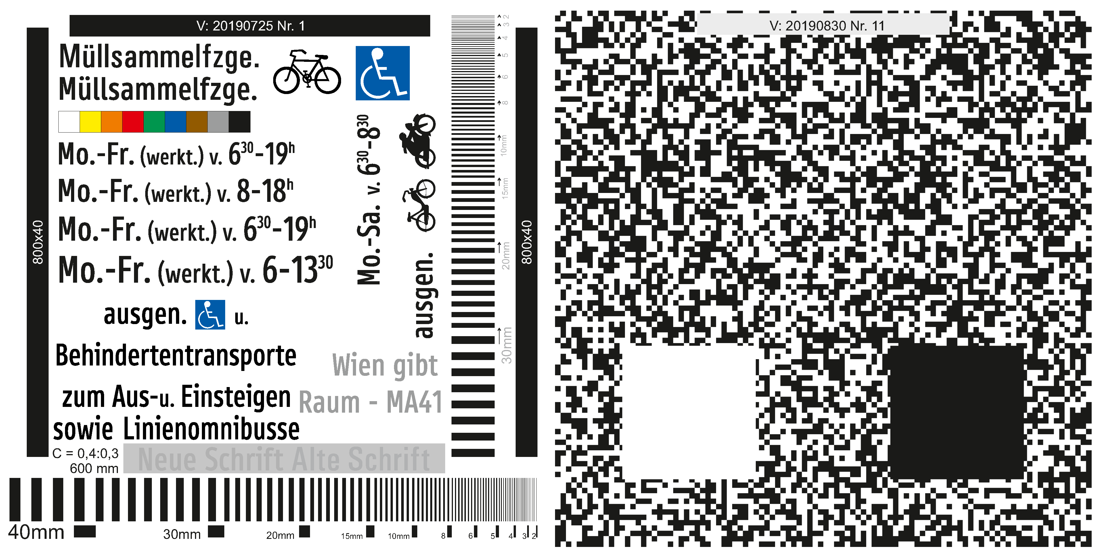
These considerations led to the test chart shown in
Figure 2 (left). There are continuous bars of 800 mm length (vertical) and a gray bar of 600 mm length (horizontal). The font sizes match the ones found on street signs (of the City of Vienna), as do the font shapes, the colors, and the symbols. The smallest font height is 40 mm, but the next bigger fonts (heights of 42 mm, 45 mm, and 50 mm) are placed on the board, too. The line pairs range from a width of 40 mm down to 2 mm. This corresponds to a black and a white line with a width of 1 mm each. The height of the line pair pattern is 80 mm. The vertical line pair pattern starts from a width of 30 mm, also because motion blur is to be expected for the horizontal direction, i.e., parallel to the driving direction, but not in the vertical direction. The text was chosen from experience and includes superscript elements (e.g., 6
30-19
h, meaning the time span from 6:30 to 19:00), individually downsized letters (e.g., Aus-u. Einsteigen, which refers to entering and exiting public transport, but ‘and’ (in German ‘und’) is abbreviated to a small ‘u.’, etc.).
The method for the evaluation selects images according to the test configuration. Since the image positions will not correspond exactly to the required distance (depending on the trigger rate of the system), the closest image must be selected, which has at least the required distance from the test chart. For each selected image, the evaluation method processes one chart element after the other. First the continuous vertical and horizontal bars are used to compute pixel size at the object. A large number of image viewing or processing programs can be used for this, as long as the program is capable of showing the pixel coordinates. From the measurement of two corners along the same long edge the distance in image space is computed and used to divide the object space distance (800 mm in
Figure 2). This leads to the pixel size at the object Δ. These values should well correspond to the nominal quantities computed from distance, focal length and pixel size in the image plane. However, there is not necessarily an orthogonal viewing direction onto the chart, thus these values may differ.
Next, the line pair patterns are analysed and the smallest line pair width w, for which the black and the white bar can definitely be discriminated is used to define the resolution limit at the distance from test chart to driving axis. The measures for vertical and horizontal resolution, and shall be noted as different values, because motion blur will rather decrease the resolution of the standing bars than of the lying bars.
Following, legibility of text and symbols is determined. To diminish possible effects of personal bias, it is determined by a jury of three people. A check list of which elements are recognizable or not, needs to be generated in advance and processed in that order. Concentration is put on difficult cases (e.g., text “Mo.-Fr.”, “(werkt.) v.”, superscript “h” and superscript of minute specification for a certain text size). For longer words we suggest to firstly concentrate on particularly difficult letter combinations and secondly on the words in their entirety (double-l, and then “Müllsammelfzge.”, garbage trucks). If foreseen, this is followed by assessing text legibility at reduced contrast, larger fonts, and finally by recognizing details of symbols or symbols in their entirety.
3.3. Point Distribution: Test Chart and Evaluation Method
A second test chart is suggested for assessing the point density and point distribution. It is known that certain measurement technologies have drawbacks at certain surface types or with certain texture (e.g., surfaces with special reflection behavior, geometrically not well defined surfaces, etc., see e.g., [
34]). A test of point density should not be influenced by these reflectance issues but rather allow to assess the point density in typical situations. Furthermore, in urban areas there are mainly diffusely reflecting surfaces, although man-made surfaces may feature more “problematic” surfaces than found in natural areas (retro-reflective surfaces, strongly absorbing surfaces, smooth surfaces leading to mirror-like reflection, surfaces without texture, porous surfaces, wires), but also water surfaces can pose problems (e.g., multi-path due to mirror-like reflection). Thus, a random binary black-white pattern is suggested. The spatial frequency of the pattern should be well beyond expected or required values for point density. One larger square in black and one in white is included in the lower part of the chart to understand the point cloud behavior at very bright and very dark surfaces without texture (e.g., biased measurement of range, no points, etc.).
These considerations lead to the test chart shown in
Figure 2 (right). It consists of a random black-white-pattern with 100 pixels over an edge length of 1 m. This may not be sufficient for applications such as street surface inspection, as tasks such as crack detection may require higher resolution, e.g., with road GSD (ground sampling distance) in the order of 1 mm [
35].
Point density is measured in number of points per unit area. This does not consider the distribution of points within the area. A high density of points along a single line could still lead to a very high point density, without the ability to properly reconstruct the surface from a sparse set of densely sampled lines. Thus, also measures of point homogeneity are necessary to assess the quality of the point cloud distribution. However, an inhomogeneous distribution per se is also not bad, as long as the density in different (orthogonal) directions is sufficiently high. In such a case the number of points along one direction may be much higher than necessary whereas in another direction it just fulfills requirements. Therefore, the proposed method does not only determine point density as number of points per unit area, but also measures local point distribution per point and analyzes the distribution of those values.
The specification of point distribution therefore consists of a global point density (number of points per unit area), and of a local inhomogeneity measure, described by a factor. The density
is determined by manually selecting a large area within the point cloud over the test chart. This area should only include the random black white pattern and neither the border nor the large white or black square shown in
Figure 2 (right). This area would typically be 0.5 m
2. For the selected points the orthogonal regression plane is determined and the area of the selection polygon is determined by the projection of the polygon vertices onto that plane. A robust fitting procedure is a possible alternative, but because of the manual selection not deemed necessary. The density
is then the number of points in the polygon divided by its area. This can be tested against a threshold
. The linear point distance is computed as
and
, respectively.
The homogeneity is determined by projecting the points selected in the previous step onto the adjusting plane. A coordinate system is chosen arbitrarily. For each point the distance to the nearest neighbor per quadrant is computed, and those 4 distances are sorted ascending. From the distribution of 1st-, 2nd-, 3rd-, and 4th-nearest neighbor distances the median is taken, named
. The inhomogeneity factor is defined as:
This could be tested against a threshold, e.g., . Obviously, if and the inhomogeneity does not matter, because both distances are smaller than what would result from a regular square distribution of points with threshold distance .
The precision, finally, is determined by a measure of the dispersion of the residuals from the regression plane estimation. Two options are the standard deviation of the residuals and a robust measure based on the median of the absolute deviations from the median (
). We suggest to use the latter one. Code for computing these values is given in the
Appendix A.
4. Experimental Evaluation
The test charts and evaluation methods described above can be used to evaluate the performance of mobile mapping systems. A specific test configuration mimics the application scenario and requirements originating in the intended applications (e.g., digitizing street sign text at a certain distance). It therefore defines which quality parameters have to be reached at which distance between vehicle and object, under which viewing directions, and at a prescribed vehicle speed. The trajectory of the mobile mapping vehicle (position and angular attitude as function of time) allows verifying these conditions. A test configuration therefore consists of location and orientation of test charts, the route the vehicles has to drive relative to the test charts and setting of thresholds for the criteria on imaging and point cloud quality. Not only the time frame for a test, but also the test configuration should be communicated to test participants in advance.
Note that the test configuration also prescribes a certain configuration of the mobile mapping system itself, e.g., that images are acquired in forward, side-ward and backward looking directions. In the case of the City of Vienna, panorama images were explicitly required.
4.1. Test Configuration
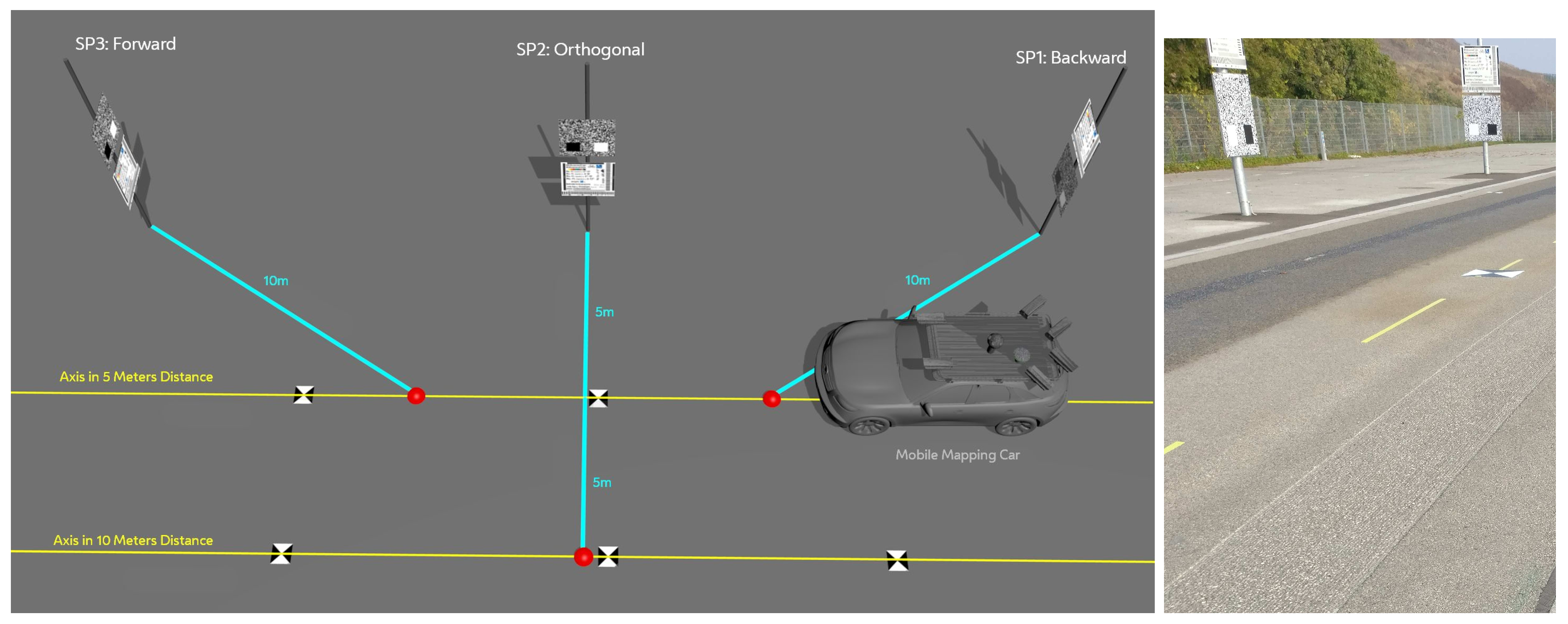
One test configuration is shown in
Figure 3. Three pairs of test charts, see
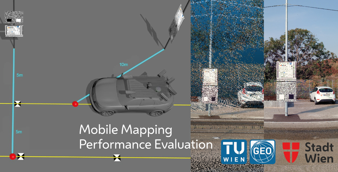
Figure 2 left and right, are placed along a line. The chart pairs are oriented once parallel to the line and twice orthogonal to it. With a speed of at least 40 km/h the mobile mapping vehicle drives once along two straight lines, which are in distances of 5 m and 10 m, respectively, of the test charts. This allows an oblique forward and backward view on the charts, which corresponds to the typical view of drivers on street signs, but it is also comparable to a view into a side street and pedestrian viewing directions. Speed and distance are chosen rather high to allow fast acquisition. Traffic shall not be disturbed by the measurements, and also over longer distances signs should be legible, i.e., across driving and parking lanes and side walk. The speed of 40 km/h was reached in a first campaign for the street network of the City of Vienna.
To keep the distance while driving as exactly as possible, it is recommended to mark the axes on the ground. In addition, clearly visible control points should be provided for accurate georeferencing. For the later evaluation of the data it is important to survey the test configuration (e.g., corner points of the charts, control points on the ground, driving lanes).
A small number of mobile mapping images of test charts are analysed. An image consists of the image matrix in a standard format, e.g., TIFF and JPG, and its exterior and interior orientation, as well as meta data comprising pixel size, aperture opening, acquisition date and time, etc. For the specific test presented below, three images are analysed. The fist image comes from the drive by at a distance of 10 m. It is used for the orthogonal view onto the test chart. Depending on the location of the camera on the car, this may correspond to a distance between camera and test chart of a bit more or less than 10 m. Additionally, one forward looking and one backward looking image are analysed, both have a distance of not less than 10 m from the corresponding chart. The point clouds from the 5 m and 10 m drive are provided as las- or laz-file (
https://www.asprs.org/divisions-committees/lidar-division/laser-las-file-format-exchange-activities) and analysed independently.
4.2. Test of Mobile Mapping Systems
In an experimental evaluation different mobile mapping data providers participated in a test. The configuration is as described above. The following criteria were evaluated. The threshold values given are indicative and not necessarily identical to the requirements of the City of Vienna.
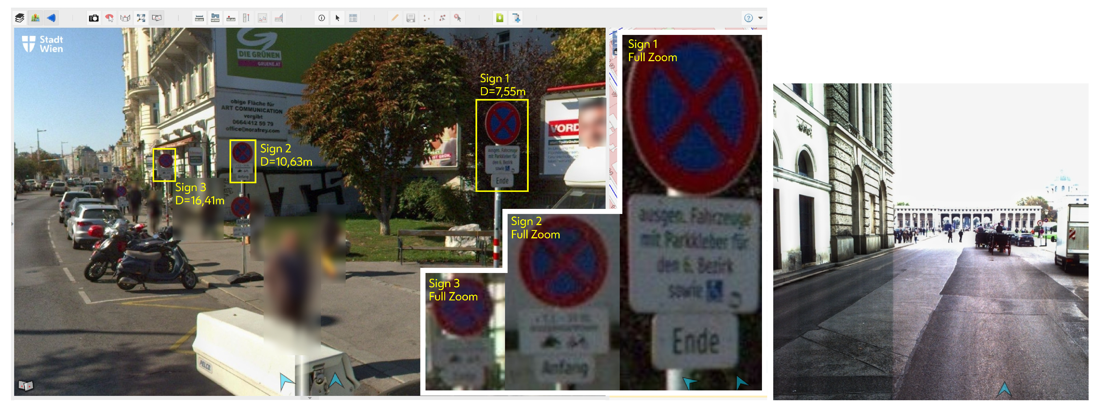
Legibility of the signs at a certain distance in certain viewing directions (e.g., 5 m or 10 m distance, in forward, backward and side-wards view): This is evaluated for the text size of 4 cm, which is the smallest text size found at traffic signs in the City of Vienna. Legibility is evaluated for the text line “Mo.-Fr. (werkt). v. 630-19h”, for “Müllsammelfzge.” in two different fonts, for the text block “ausgen. […] Linienomnibusse”, including one symbol, and the vertical text block “Mo.-Sa. v. 630-1830 ausgen.” augmented by two symbols. Each symbol is treated like a letter. Marks are given, a if each letter alone can definitely be read, b if the text is legible, and c if the text is not readable. This evaluation is executed by a jury of three persons with experience in quantitative retrieval of geometric information from images.
Pixel size at the object at 10 m distance, in forward, backward and side-ward view, smaller than (e.g.,) 5 mm: This is evaluated with the vertical 800 mm bars (average of two) and the grey horizontal 600 mm bar.
Resolution at the object at 10 m distance, in forward, backward and side-wards view, allows at least identification of the 20 mm wide black white line pairs: This is evaluated independently for the vertical and horizontal pattern of black-white line pairs of varying width.
Point density at least (e.g.,) 3000 points per m2 at 5 m distance in side-wards view: This is evaluated with the second test chart using a large polygon within the random pattern part. The points inside this polygon are also used for the subsequent two tests.
Precision of the point cloud better than (e.g.,) 15 mm at 5 m distance. This is evaluated with the of the deviations of the selected point cloud set from the orthogonal regression plane.
Point distribution homogeneity better (i.e., lower) than 2.0: This is evaluated with the factor
f (Equation (
1)) determined for the selected point cloud set.
Other elements of the test charts were not evaluated (e.g., legibility at reduced contrast, representation of color).
4.3. Results
Three mobile mapping systems were evaluated using the procedure described in
Section 4.2. These three mobile mapping systems collect images. Point clouds are either provided by laser scanning or by dense image matching.
Panoramic camera images were evaluated, as these were intended for the later use. The systems were specified by the service providers. It is noted that some of the systems also provide standard frame camera images which may feature a higher resolution than the panorama camera at a reduced opening angle. Depending on the intended use, frame camera images with a certain viewing directions or panorama images may be preferred. One system has the panoramic image of a Leica Pegasus: Two Ultimate (24 Megapixel), and provides point clouds from a LiSAR, the Zoller+Fröhlich Profiler 9012 (measurement rate of 1MHz with a rotation speed of 200 Hz). A second system uses a large panoramic camera system with a total of 250 Megapixel and a Velodyne HDL-32E LiDAR for the point clouds (measurement rate of 0.7 MHz). A third system uses a panoramic camera system with a total of 30 Megapixel and the point cloud is provided by dense image matching.
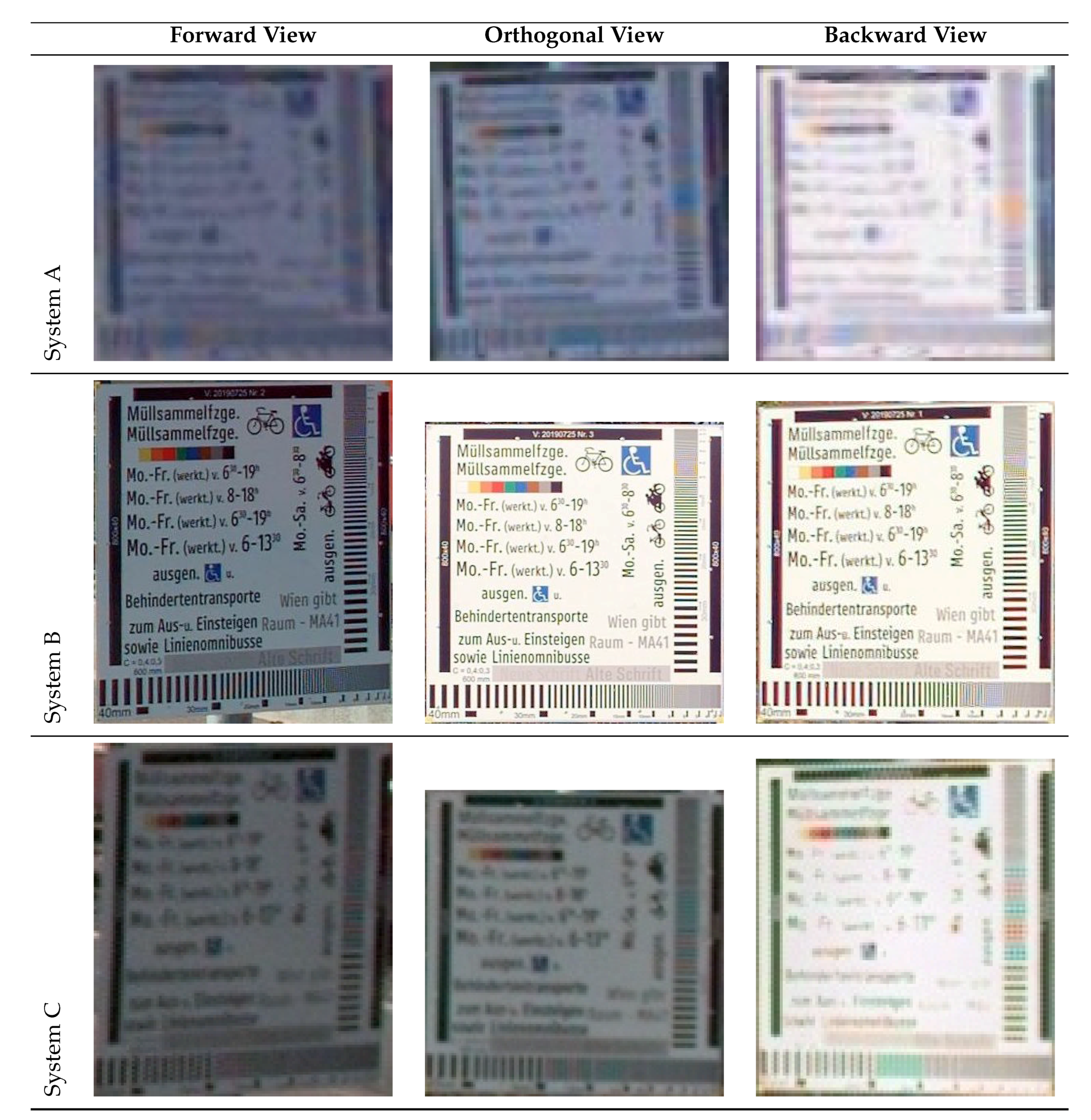
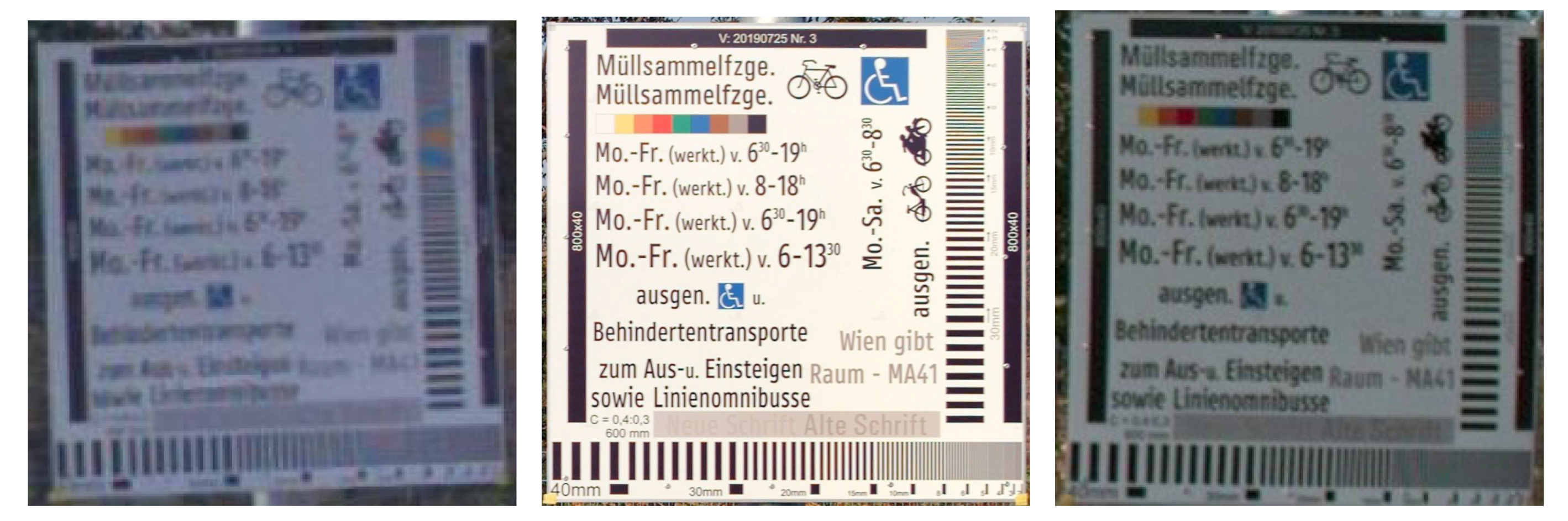
In the results presented here, it is not checked, if the criteria are met, i.e., not a binary decision is reported, but rather the respective quality parameter is given. More quality measures than feasible in a tendering procedure are evaluated. The photos at 10 m distance of the test charts for imaging quality are shown in
Figure 4, photos at 5 m distance are shown in
Figure 5. The point clouds at distance of 5 m of the test chart parallel to the driving direction is shown in
Figure 6. The results are given in
Table 1 for image quality. In
Table 2 the point cloud parameters are given for the orthogonal chart from a distance of 10 m and 5 m. The point clouds of the middle test charts are visualized in
Figure 6.
4.4. Analysis
The measurements performed in the test charts were successful. Independent thereof, several observations were made.
The jury of three people could come to a unanimous decision within short time (less than a minute per case), and the situation was always obvious. For the 10 m charts this is visible in having only decisions a and c.
Repeated measurements of bar lengths were used to compute the precision of the estimated pixel size. For all assessed lengths a standard deviation below 1 pixel is reached and the maximum difference between shortest and longest length reached 4 pixel during the repeated measurements. As it was to be expected, images with higher quality featured better precision.
Repeated determination of the line pair width that can still be identified, gave different values from different individuals. However, in the (absolute) majority of cases the same width was identified. In all other cases the decision was to be made between two neighboring widths. The 8-fold repetition of the black-white pattern was helpful for determining, if the pattern can be uniquely identified or not. We also note that severe color distortions become visible in the bar patterns at the resolution limit and beyond it.
The design of the test chart was following the requirements of the City of Vienna. However, some of the evaluated systems could not reach the minimum given at the test chart. This suggests a redesign of the charts to offer quantitative results for a wider range of systems.
Measurements of the grey horizontal bar clearly demonstrated, that lower imaging resolution and low contrast at the object can lead to barely legible signs. For improving the accuracy of pixel size assessment, a black bar should be used instead of a gray one. However, it must also be stressed, that the image quality achieved in the test is applicable to mobile mapping street space acquisition only under good conditions for photography (sufficient light) and at clean objects.
Repeated assessments of the point cloud, using different selections of the point cloud, lead to a variation of the density and precision measures. For the lowest density example (B @ 10 m) five repetitions lead to a variation in point density below 1% and the range of precision values was below 1 mm. Medians of the neighborhood distances showed no variation.
The numbers given in the above tables correspond to the emphasis the different vendors put on the mobile mapping systems. Although the first aim of the research was to develop and test an evaluation method, the results for the three mobile mapping systems allows characterizing those three specific systems.
System A has, according to vendor specifications, better cameras for forward and backward view, e.g., for reading overhead signs for drivers. The quality of those images was not assessed (the images were not available), as this was not part of the test for city-wide data acquisition of street space. The panorama image provides lower quality. The laser scanner is mounted to scan one plane inclined against the driving direction, which is appropriate for assessing the surface of individual street lanes. Also the laser scanning accuracy fits to such an application. Likewise, depends on the distance between sensor and object, whereas depends on driving speed.
System B is the best among the investigated systems for assessing the entire streets space visually, providing hemispheric images of the highest quality. It provides the best images for reading street signs. The Velodyne laser scanner provides better resolution in both directions when scanning at shorter distance. However, the precision is notably lower. Point clouds appear not to be the primary product from this mobile mapping system.
Finally, System C is in the middle of the previous two systems, providing imaging quality between Systems A and B. As the point clouds originates from dense matching, the precision notably decreases with distance from the target. Also ghost points appear next to edges whereas wires are not reconstructed. While the capability of the mobile mapping systems to acquire point clouds of wires was not part of the test,
Figure 6 strongly suggest to include such an assessment, should it be in the scope of the applications.
It is noted here, that quantitative performance indicators are provided by the test, which allows comparing each system to predefined requirements.
To demonstrate the usage of these quantitative performance metrics assume that a city-wide acquisition should be performed with a system that provides images where street signs with 4 cm text height at 10m distance in various directions can be read and that delivers point clouds with a density of 4000 points/m2 with a precision of 5 mm. In that case, non of the investigated systems can be chosen. In a second example, requirements are lower and images parallel to the street at a distance of 5 m with text height of 6 cm need to be legible and point clouds with a precision of 10 mm and a density of 2000 points/m2 at 5 m distance need to be provided. In this scenario two systems could be chosen, and the price may become decisive.
This test configuration is compatible with mobile mapping systems taking standard frame camera images or spherical images, i.e., area images with individual projection centers. For line camera images the test charts may still be useful. The test configuration is applicable to systems providing point clouds from laser scanning or from image matching. The test configuration also allows evaluation of the absolute georeferencing accuracy if the test charts (and other elements in the scene) are surveyed accordingly. However, a longer track should be used for such a test.
From a methodological point of view, a new measure for assessing point distribution was suggested. Two values are suggested to characterize it, and , which ‘fits’ to surfaces, which are bivariate functions. The suggested measure has the underlying assumption, that local inhomogeneity does not change drastically within the investigated area (e.g., holes of data, or large differences in inhomogeneity at very different scales). For the very regular point distribution of system A, the values correspond well to direct measurement in the point cloud. Systems B and C provide an irregular point distribution, which cannot be formalized.
The total effort for executing the test was low. The cost for generation of each board was EUR 1 000 (3 mm aluminum plate, including retro-reflecting coating for boards with text and diffusely reflecting coating for point distribution boards and corresponding mounting clamps). Mounting the boards, marking lines to drive along, surveying the test area with a total station etc., was two days for two persons. This effort needs to be made once. For each test, data selection and analysis (selection of images, cutting point cloud, identification of resolvable line pair width, computation of pixel size, etc.) took approximately half a day per test for one person. Obviously, it would be possible to automate parts of this evaluation further. As all the data is georeferenced, preselection of data could be implemented. To become independent of georeferencing errors, coded targets are an alternative.
5. Conclusions
We presented test charts for mobile mapping images and point clouds. The test charts are portable because of their dimensions (1 m by 1 m), but the test was performed with a fixed installation. Two test charts were suggested, one for assessing imaging quality containing line patterns of different width and text as typically found on street signs. The other chart contained a random black white pattern to assess point cloud properties. A complete testing procedure consists of a route the mobile mapping vehicle drives along with a defined speed, the placement of the test charts along this route, and a set of parameters to be extracted from the point clouds and images showing the test charts.
The tests could be executed as planned in a ‘real world’ environment. We conclude from this, that the charts and the testing procedure are—at least for the investigated systems—suitable. The effort for testing additional systems is moderate and mostly lies on the data providers, because a (small) project has to be executed. The evaluation itself uses simple means (image viewer) and standardized processing (see
Appendix A). Our aim is to extend this investigation by testing more mobile mapping systems. An important extension of the test to characterize the urban space more comprehensively would be to quantify the performance of different systems on wires. As for the current criteria, this should be driven by application requirements. We furthermore think that such a test can also be very interesting for system vendors, system integrators, and service providers. Independent of tendering procedures or specific projects, it allows quantifying system quality independently.
The investigated mobile mapping systems show diverse characteristics. This is interpreted as a specialization of these mobile mapping systems for different tasks: acquisition of the entire street space (in the sense of the public space used by pedestrians, cars, etc.) vs. acquisition of the driving space (lanes, signs for car drivers). The concentration on panorama images and point clouds in the presented test, as well as the selection of tested parameters, gives relevant insight into characteristics of the investigated mobile mapping data sets, but is not an assessment of the mobile mapping sensor systems.


