Abstract
As an important component of the urban ecosystem, street trees have made an outstanding contribution to alleviating urban environmental pollution. Accurately extracting tree characteristics and species information can facilitate the monitoring and management of street trees, as well as aiding landscaping and studies of urban ecology. In this study, we selected the suburban areas of Beijing and Zhangjiakou and investigated six representative street tree species using unmanned aerial vehicle (UAV) tilt photogrammetry. We extracted five tree attributes and four combined attribute parameters and used four types of commonly-used machine learning classification algorithms as classifiers for tree species classification. The results show that random forest (RF), support vector machine (SVM), and back propagation (BP) neural network provide better classification results when using combined parameters for tree species classification, compared with those using individual tree attributes alone; however, the K-nearest neighbor (KNN) algorithm produced the opposite results. The best combination for classification is the BP neural network using combined attributes, with a classification precision of 89.1% and F-measure of 0.872, and we conclude that this approach best meets the requirements of street tree surveys. The results also demonstrate that optical UAV tilt photogrammetry combined with a machine learning classification algorithm is a low-cost, high-efficiency, and high-precision method for tree species classification.
1. Introduction
The rapid urbanization of China over the past three decades has resulted in major environmental challenges, among which air pollution, the urban heat island effect, and noise pollution are the most prominent [1,2]. The inhabitants of urban environments are increasingly exposed to severe environmental pollution, which may critically affect their health and daily activities [3]. As interest in environmental and health issues has grown, urban environmental health and living comfort are attracting increasing attention. In this context, the urban vegetation system is important for urban environmental protection and for improving the urban climate [4,5]. As a component of the urban vegetation system, street trees play an important role in urban greening and in urban environmental improvement [6]. Tree species identification is an important aspect of street tree research [7,8], and accurate and rapid tree species information is necessary for various aspects of street tree management.
In traditional forest management, tree species classification is mainly conducted via manual visual interpretation, and its classification accuracy depends on the professional knowledge of the operator; moreover, the method is time-consuming, laborious, and inefficient. However, with the development of remote sensing, many cutting-edge remote sensing technologies have been applied to tree species classification, greatly improving its efficiency and accuracy [9,10,11,12]. High-resolution remote sensing data were first applied to large-scale tree species identification, demonstrating its potential for classifying tree species based on various forest characteristics [11,13]. However, urban tree species differ from those in planted and natural forests, and in addition, the urban background is complex and the biodiversity is high. As a result, the classification accuracy of urban tree species based on pixel-based high-resolution remote sensing data is relatively low [14]. Hyperspectral remote sensing data contain rich spectral information and, combined with airborne lidar, they can distinguish tree species with similar spectral information; this approach is also highly accurate and, for these reasons, it is often used to classify forest tree species [15,16]. However, because of the complexity of the urban environment, this method does not provide detailed information about the understory. Because of its high positional resolution, rapid scanning speed, and simple source of error, Lidar is used for tree species identification [17,18,19]. Lidar data and hyperspectral data complement each other well, and their combined use can provide spectral information on trees, as well as high-precision morphological information, which enable the identification of individual tree species with high accuracy [20,21,22]. Although this approach has a high recognition accuracy, it is difficult to apply it widely because of its high cost and complex operation.
Because of the increasing need for classification accuracy, more algorithms are being applied to tree species classification. Among them, K-nearest neighbor (KNN), random forest (RF), support vector machine (SVM), and neural networks in machine learning are widely used in tree species classification [23,24]. The machine learning classifier uses the spectral information between different tree species, or the difference in the point cloud structure model, to classify tree species, and it has been shown to provide better practical results than other algorithms [25,26,27]. In order to provide higher-precision classification results, deep learning is increasingly being applied to tree species classification, and deep learning algorithms can achieve end-to-end feature extraction, which can minimize feature loss. Among them, the classification accuracy of 3D-CNN, ResNet, and other convolutional neural networks in hyperspectral, multispectral, and optical data can reach an accuracy of more than 90% [28,29]. PointNet++ for point cloud data classification has also been applied to tree species classification with very promising results [30,31]. However, compared with the more convenient and efficient machine learning, deep learning is difficult to apply widely in forestry investigation because of its large training sample size, slow speed, and the high degree of difficulty in model training.
In recent years, unmanned aerial vehicle (UAV) photogrammetry technology has emerged and is being widely used in surface modelling, determination of coastline, geological survey [32,33,34], and so on. Tilt photography technology is a relatively recent high-tech development in the field of international surveying, mapping, and remote sensing. The technique of tilt photogrammetry is an automated method for constructing 3D models that greatly improves the efficiency of 3D modeling [35,36]. Tilt photogrammetry is capable of collecting image data from multiple angles such as vertical and tilt for the same drone, in order to provide complete and accurate texture data and positioning information. The resulting rich and colorful image information provides more realistic visual effects compared with the 3D model, and it eliminates the cost of 3D modeling [37]. Thanks to its advantages of mobility, flexibility, low cost, and high safety, it has been widely used in forestry investigations [35,38,39,40]. Tilt photogrammetry can rapidly and efficiently generate high-precision three-dimensional models of trees from different angles, accurately reflecting their three-dimensional structure. Compared with Lidar, photogrammetry has greater requirements for light, and because the optical sensor has low penetration, the accuracy of Lidar is lower when it is required to reflect the internal structure of trees, compared with high-precision three-dimensional modeling [41]. However, compared with hyperspectral and lidar data, UAV tilt photogrammetry has the advantages of simplicity of operation, high efficiency, and low cost [42]. In forestry investigations, the requirements for work efficiency and cost are often greater than the requirements for accuracy; therefore, photogrammetry is likely to be the most popular method in future forestry surveys.
In the present study, we have developed a tree species classification method based on UAV tilt photogrammetry. The approach uses drone tilt photogrammetry to generate a three-dimensional point cloud model of trees, enabling tree attributes to be extracted. Combined with the classification algorithm method of machine learning, it can provide effective tree species identification with high efficiency in terms of time and cost.
2. Study Area and Data
2.1. Study Area and Data Acquisition
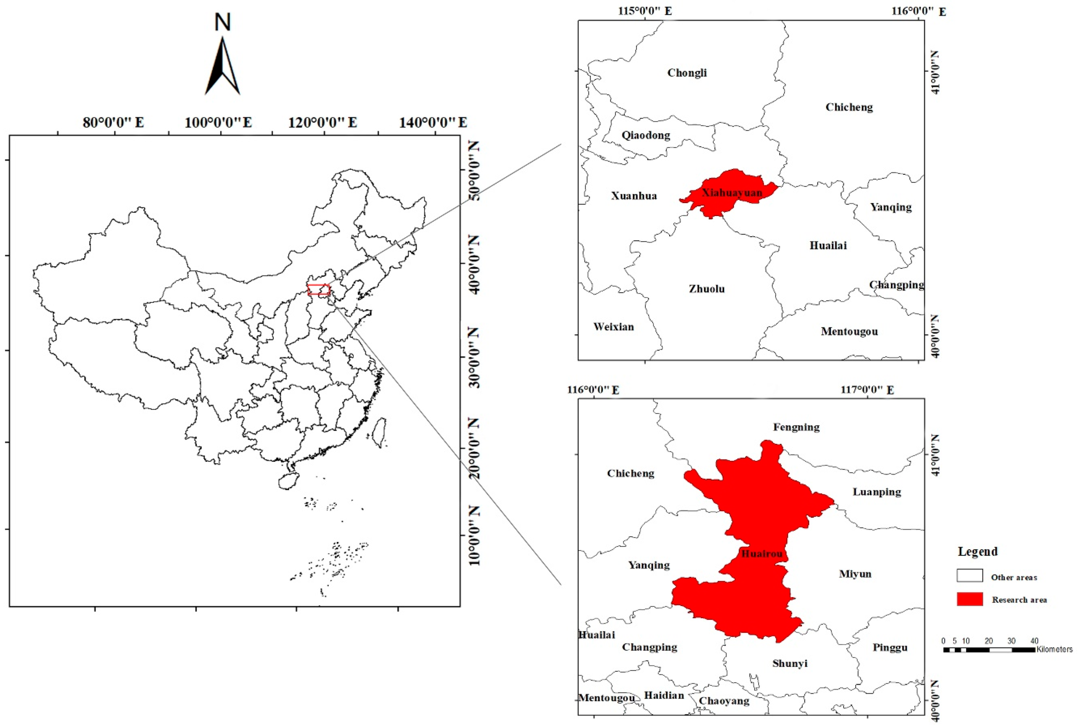
The selection of the study areas was based on three criteria: (a) the street trees should be representative of similar areas elsewhere; (b) they should be far from tall buildings and be free from interference by strong magnetic fields; and (c) they should not be no-fly zones for drones. After several on-site inspections before deploying a drone, and after comprehensively considering the above factors, we selected the Huairou District of Beijing (116°37′E, 40°20′N) and the Xiahuayuan District of Zhangjiakou City in Hebei Province (115°16′E, 40°29′N) (Figure 1) as study areas. A total of seven roads were selected in the two areas, and for the roads, an experimental plot of 50 m in length was selected. The morphological attributes of trees change as they mature; therefore, the street tree species selected in this study were mature. Mature trees grow relatively slowly and the species selected would not have changed significantly over 2–3 years. The main species of street trees in the experimental areas are Fraxinus pennsylvanica, Ginkgo biloba, Robinia pseudoacacia, Acer negundo, Populus tomentosa, and Koelreuteria paniculate.
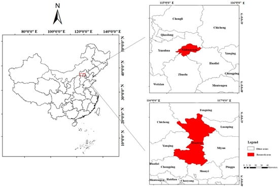
Figure 1.
The study areas and their location in China.
An unmanned aerial vehicle (UAV) was deployed in October 2019 and August 2020, when the weather was fine and the wind speeds were low. In order to avoid the influence of light conditions on the results, daily flight times of 10:00 and 14:00 were selected for optimal light conditions. To ensure the accuracy of the UAV survey, the flying height was set to 30 m, the heading overlap was 80%, and the side overlap was 80%. The data acquisition platform was the DJI (Da-Jiang Innovations, Shenzhen, Guangdong, China) Phantom 4 RTK (Real Time Kinematic) consumer multi-rotor UAV (Figure 2a). The specific parameters of the UAV are listed in Table 1, and the flight route diagram is shown in Figure 2b.
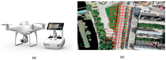
Figure 2.
Unmanned aerial vehicle (UAV) and flight route map. (a) DJI (Da-Jiang Innovations, Shenzhen, Guangdong, China) Phantom 4 RTK (Real Time Kinematic) used in the study. (b) Schematic diagram of the flight path, taking sample plot 4 as an example.

Table 1.
Basic parameters of the unmanned aerial vehicle (UAV).
2.2. Data Preprocessing
Pix4Dmapper (Pix4D, Lausanne, Switzerland) was chosen for aerial image processing; it is fully automated and can rapidly process thousands of images into professional and accurate 2D maps and 3D models. The software uses the principles of photogrammetry and multi-eye reconstruction from aerial photos to rapidly build a three-dimensional model to obtain point cloud data and perform post-processing.
The DJI Phantom 4 RTK provides real-time centimeter-level positioning data. Taddia et al. tested the root mean square error (RMSE) of DJI Phantom 4 RTK tilt photogrammetry data with and without image control points, and the results showed that the difference in RMSE between the two was only 0.003 m [43]. The measurement results of the UAV with and without ground control points used under RTK GNSS (Global Navigation Satellite System) are very similar, and the error between the two is small. In order to reduce the error caused by the lack of ground control points, the flying height was set to 30 m. The present study was intended as a pilot study before conducing a large-scale experiment. An important goal was to find high-efficiency and low-cost methods of tree species identification; therefore, in order to improve work efficiency, we rejected the use of ground control points. After importing the image data obtained by tilt photogrammetry into Pix4Dmapper, the software automatically reads the image pos information, and then the tilt photogrammetry modeling method and the coordinate system and projection are set; the default used is the WGS 84/UTM zone 50N projection coordinate system. The software automatically performs initialization and three air three encryption operations to generate a three-dimensional model; the generated 3D model of the plot is then converted to a 3D point cloud form. In the point cloud mode of the Pix4D-mapper software, the point cloud editing tool was used to manually separate single trees and split the single tree, and only the tree point cloud part of the plot was retained; a voxel-based outlier filter was then applied to remove the discrete points [44].
3. Methods
The single tree attributes of different tree species are quite different, and those of the same tree species are similar; therefore, tree species are classified according to the differences in attributes between different species. The experimental steps for achieving this were as follows: (i) extraction of single tree attributes and accuracy verification; and (ii) selection of different machine learning classifiers for tree species classification, and comparison and analysis of the classification results to select the best classifier. The complete workflow is illustrated in Figure 3.
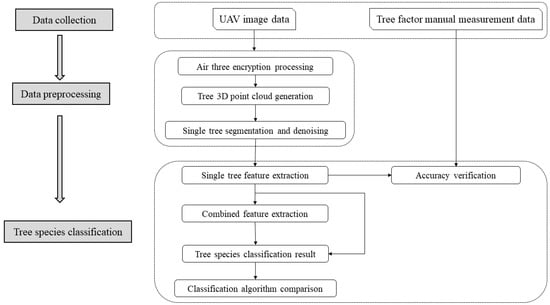
Figure 3.
Complete workflow from field data collection to tree species classification.
3.1. Extraction of Indivual Tree Attributes
According to the individual tree point cloud characteristics, individual tree attributes (tree height, crown height, crown, width and crown volume) were extracted from the single tree point cloud data obtained by tilt photogrammetry; these attributes were then used for tree species identification [45,46].
3.1.1. Tree Height Extraction
Tree height refers to the distance or height of the tree, from the roots on the ground to the top of the crown [47]. A rectangular coordinate system was established based on the tree point cloud. In the complete standing tree point cloud data, the top of the standing tree is its maximum value in the Z-axis direction, and the base is the minimum value in the Z-axis direction; therefore, the tree height is the difference between the two in meters (m):
3.1.2. Crown Width Extraction
In forestry management, the crown width is generally divided into the east–west width and the north–south width, according to the direction of the crown width. Because the point cloud data generated by the PIX4D software is in WGS84 coordinates, the X-axis and Y-axis directions of the point cloud data in the three-dimensional coordinate system correspond exactly to the east–west and north–south directions in geographic coordinates. When using the point cloud data to calculate the crown width, the crown point cloud is projected onto a two-dimensional plane, and the maximum distance in the X-axis direction of the projection surface is calculated as the east–west crown width, and the maximum distance in the Y-axis direction as the north–south crown width:
Here, , , , and are the maximum and minimum values of the canopy projection plane in the X-axis and Y-axis directions, respectively, in meters (m).
3.1.3. Crown Height Extraction
In traditional measurements, the problem in measuring crown height is how to distinguish the lowest part of the crown. If the base of the canopy is relatively complex, determining the lowest part requires careful observation. In this study, we used the principle of threshold segmentation to segment the tree crown and trunk three-dimensional point cloud. The threshold segmentation used in point cloud segmentation is commonly used to determine the maximum between-class variance. Assuming that the threshold is between the maximum point and the minimum point , the threshold t divides the point cloud into two parts: the canopy point cloud (C) and the trunk point cloud (T). Therefore, the inter-class variance of the two types of point cloud height divided by the threshold is calculated as follows:
Here, is the proportion of the point cloud of the canopy in all point clouds, is the proportion of the point cloud of the trunk in all of the point clouds, is the average height of the tree point cloud, is the average heights of the canopy point cloud, and is the mean value of the point cloud of the trunk. According to the optimal threshold selection principle, when is at a maximum, the value of t is the optimal threshold; in this case, the crown height is calculated as follows:
3.1.4. Canopy Volume Extraction
The use of tree point clouds to calculate the crown volume requires the use of the threshold segmentation method to extract the individual tree crown, followed by the voxel method to calculate the crown volume [48]. The basic principle of the voxel method to calculate the crown volume is to divide the crown into numerous small cubes. Choosing a suitable voxel can reliably simulate the crown shape and internal structure. The tree canopy is layered first; then, the line connecting the highest and lowest points of the canopy is taken as the Z-axis, and the canopy is divided into n layers at intervals of k. The point cloud of each layer is projected onto the XY plane perpendicular to the Z-axis, along the X-axis and the Y-axis divide voxels at intervals of k. In calculating the canopy volume, it is necessary to assess whether it contains a point cloud by voxel on each cross section. The voxel containing the point cloud is the effective voxel and is recorded as 1, and the pixel without the point cloud is recorded as 0. Counting the number of effective pixels V in each layer, the crown volume is calculated as follows:
Here, is the canopy volume in m3; is the side length of the pixel, m; is the number of canopy layers; and is the number of effective voxels in the i-th layer.
3.2. Extracting a Combination of Tree Attributes
When training a classifier, the more attribute parameters that are used, the more often the various attributes of the classification sample can be taken into account. Therefore, in this study, we obtained multiple tree parameters via a pairwise combination based on individual tree attribute factors. The combination of parameters used can be divided into two complete tree attributes and two crown attribute parameters (see Table 2 for details), where the crown length is the average of the crown width in the east–west direction and in the north–south direction.

Table 2.
Combined attribute parameters.
3.3. Verification of Tree Attribute Extraction Accuracy
In order to verify the accuracy of the extraction of tree attributes, we compared the individual tree attributes extracted using drone tilt photogrammetry with the results obtained by traditional measurement methods. Data on tree height, crown height, and crown width were obtained by field measurement. The traditional method of calculating crown volume is to regard the crown as a regular geometric body, and then to use the field measurement of crown width and crown height as parameters to calculate the crown volume using the geometric volume formula [49]. The approximate geometry and volume calculation formulas of the crown of each tree species are listed in Table 3.

Table 3.
Approximate geometry and volume calculation formulas for different tree species.
3.4. Tree Species Classification
In order to study the effect of different classification algorithms on the experimental results, we selected four common machine learning classification algorithms for tree species classification: K-nearest neighbor (KNN), random forest (RF), support vector machine (SVM), and BP (back propagation) neural network.
In order to avoid the possibility of the verification sample affecting the accuracy of the model, we used a 10-fold cross-validation method to select the verification sample. Ten-fold cross-validation means that the original data are divided into 10 groups (usually divided equally, but sometimes a layered sampling method is used for unbalanced data), and each data subset is tested separately. The unselected nine data subsets are used as the training dataset, so that 10 models are obtained. The average of the classification accuracy of the 10 model validation datasets is taken as the accuracy evaluation performance index of the validated classifier under the 10-fold cross-validation. In order to further improve the accuracy of verification, it is often necessary to perform multiple 10-fold cross-validations, and to take the average of each verification result as the estimate of algorithm accuracy. Notably, in each individual folding cross-validation, all steps of the model training process will be executed independently; that is, each folding validation in a 10-fold cross-validation is independent of the others. In order to avoid experimental errors caused by difference in data dimensions, the data are normalized before classification.
In order to evaluate the classification accuracy of several classification models, we used three common evaluation indicators of classification accuracy: precision, recall, and the F-measure. The precision is the proportion of the samples that are paired in all samples, and the recall rate is the proportion of all positive samples that are judged to be positive samples and are indeed positive samples. The F-measure is the weighted harmonic precision of the precision and the recall value. It can be used to comprehensively consider the precision and the recall value, and it is often used to evaluate the quality of the classification model. F is calculated as follows:
where is the parameter, is the accuracy, and is the recall value.
4. Results
4.1. Accuracy of Tree Attribute Extraction
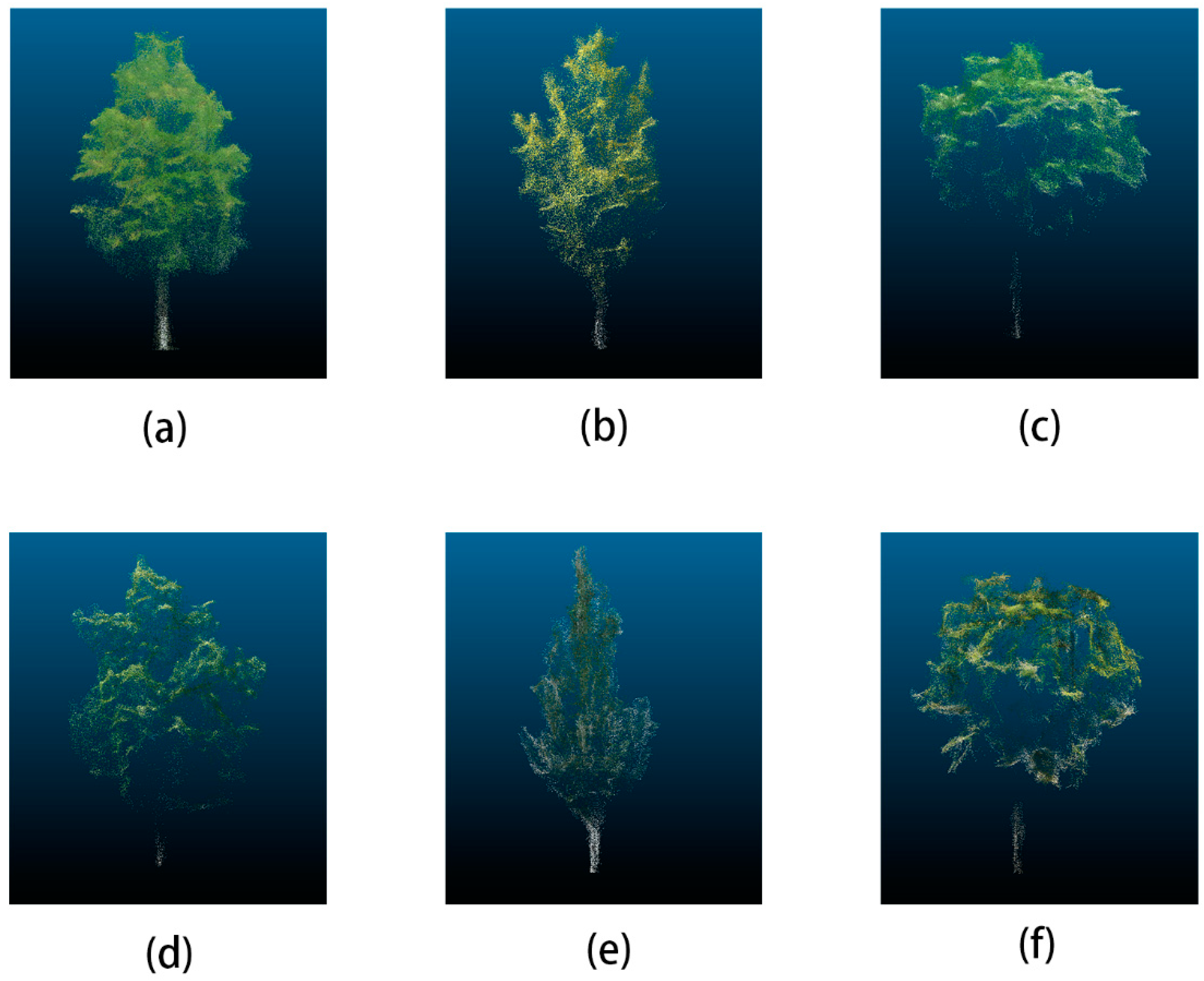
Three-dimensional modeling was performed on tilt photogrammetric images of seven sample plots obtained by field experiments; data preprocessing was performed after the modeling data points were clouded, and a total of 94 street trees comprising 6 species was obtained. The individual tree point cloud results for each tree species after point cloud data preprocessing are illustrated in Figure 4.
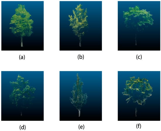
Figure 4.
Point cloud results for each tree species. (a) Fraxinus pennsylvanica; (b) Ginkgo biloba; (c) Robinia pseudoacacia; (d) Acer negundo; (e) Populus tomentosa; and (f) Koelreuteria paniculate.
Tree height, crown width, and crown height measured in the field were compared and analyzed as the true value; the results were automatically extracted by tilt photogrammetric modeling, and the absolute error and relative error between the extracted result and the true value were calculated. Because of the limitation of the measurement methods, it was impossible to measure the true value of the crown volume; therefore, here, we do not consider the extraction accuracy of the crown volume. The calculated results are listed in Table 4, from which it can be seen that the relative errors between the extraction results of the four tree attributes and the true values are all less than 20%, with the largest relative error of 16.32% for tree height. The relative error of the tree height and crown height is slightly greater than that for crown width. The maximum absolute error and the maximum average value of the four tree attributes are also for tree height, which are 4.99 m and 1.30 m, respectively. The average absolute error of crown width and crown height is less than 1 m.

Table 4.
Tree attribute extraction results.
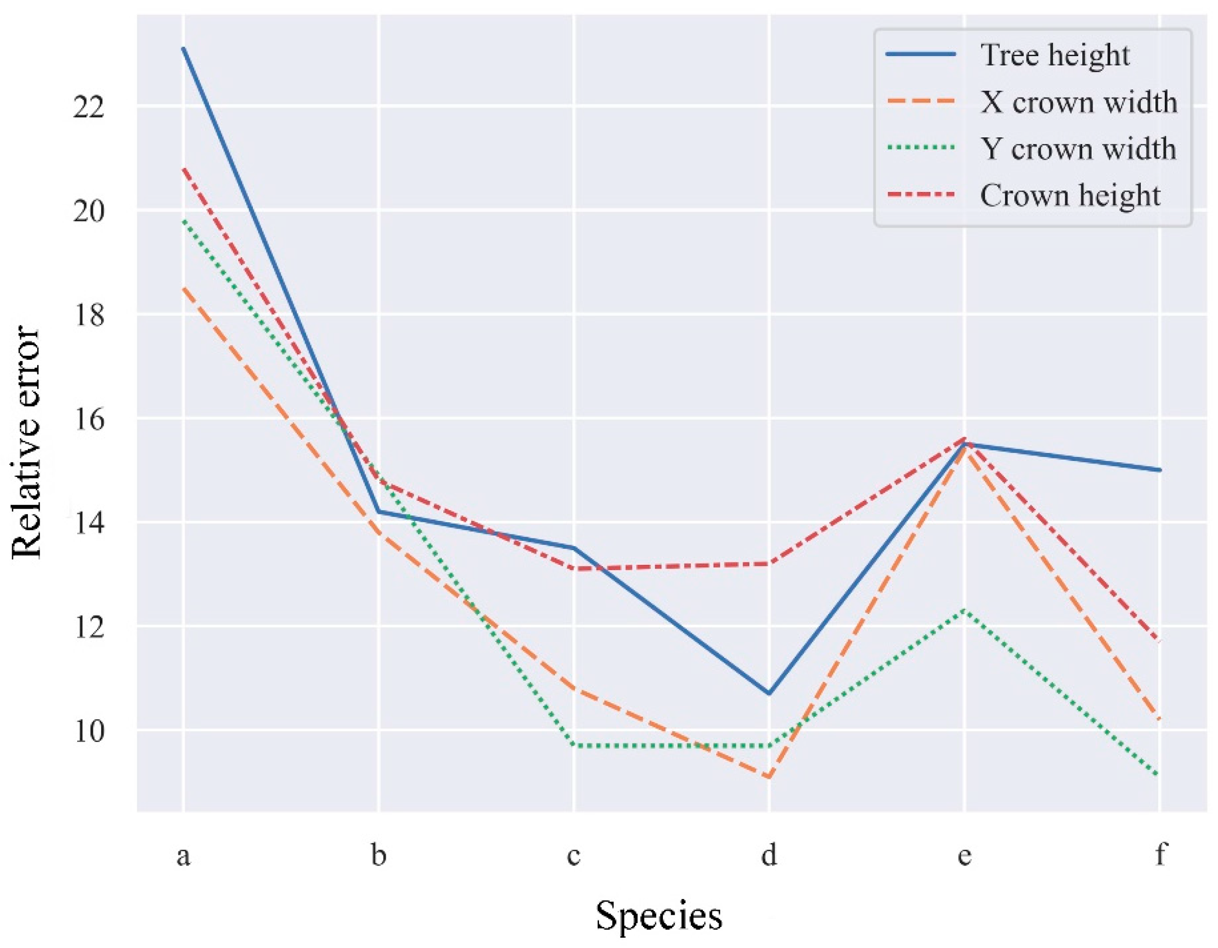
The relative errors between the tree attribute extraction results for different tree species and the true values are illustrated in Figure 5. The trend of the extraction accuracy for the four tree attributes among the different tree species is roughly the same. The species with the worst extraction accuracy of tree attributes is Fraxinus pennsylvanica, and the values are all significantly higher than for the other species. The extraction accuracy for Koelreuteria paniculate, Robinia pseudoacacia, and Acer negundo is better, with the error for each attribute being less than 14%. Therefore, combined with the calculation results listed in Table 3, we conclude that the extraction results of the tree features meet the requirements of the study.
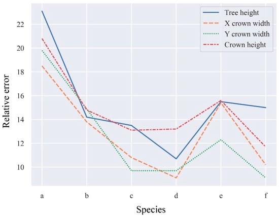
Figure 5.
Differences in tree attribute extraction results for different tree species. a, b, c, d, e, and f represent Fraxinus pennsylvanica, Ginkgo biloba, Robinia pseudoacacia, Acer negundo, Populus tomentosa, and Koelreuteria paniculate, respectively.
In order to verify whether the extraction results of tree attributes could reliably represent the structure of the trees, the correlation between each attribute and the true value was analyzed; the crown volume calculated by the geometric method was used as an optimal value of the crown volume, and the correlation between the voxel method and the ideal value was determined. It can be seen from the results (Figure 6) that the crown volume calculated by the voxel method has the highest correlation with the optimal value, with the correlation coefficient of 0.8417; this demonstrates that the crown volume calculated by the voxel method reliably reflects the shape of the crown and can be used as a key parameter for tree species classification. The individual tree attribute that is poorly correlated with the true value is tree height, with a correlation coefficient of 0.6079, and the correlation coefficient between crown height and crown width is ~0.7. The correlation coefficient between each individual tree attribute and the true value is greater than 0.6, indicating an overall good correlation and that the attributes reliably reflect the true characteristics of the trees.
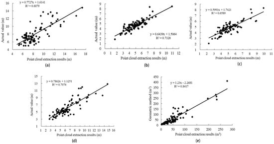
Figure 6.
Scatter plots of the relationship between extracted tree attributes and the true values. (a) Tree height vs. the true value; (b) X crown width vs. the true value; (c) Y crown width vs. the true value; (d) crown height vs. the true value; and (e) crown volume calculated using the voxel method vs. the optimal value.
4.2. Accuracy of Tree Species Classification
The five tree attributes calculated as described in Section 4.1 (tree height, crown height, east–west crown width, north–south crown width, and crown volume) were selected as training parameters for the sample trees, in order to determine whether they could provide a comprehensive representation of the characteristics of individual tree species. Four machine learning classification methods (KNN, RF, SVM, and BP neural network) were used to classify the tree species, with 10-fold cross-validation used to verify the classification. The results are listed in Table 5, from which it can be seen that, in terms of accuracy, recall, and F-value of the four classification methods, the best classification result is achieved by the BP neural network, with a precision of 85.7%, recall of 84.0%, and F-measure of 0.843. This is followed by random forest and KNN, with a precision of ~77.4% and F-measure of ~0.76. The worst classification result was provided by SVM, with a precision of only 46.3% and F-measure of 0.464. The classification accuracy for different tree species is quite different. The four classification methods achieved good results for Populus tomentosa and Ginkgo biloba, with precision rates above 80%. However, the classification results for Acer negundo and Koelreuteria paniculate are poor, and the accuracy of the four classification methods is less than 80%, with the accuracy of SVM for these two tree species being especially low (0%).

Table 5.
Classification results of different algorithms. RF, random forest; BP, back propagation; SVM, support vector machine; KNN, K-nearest neighbor.
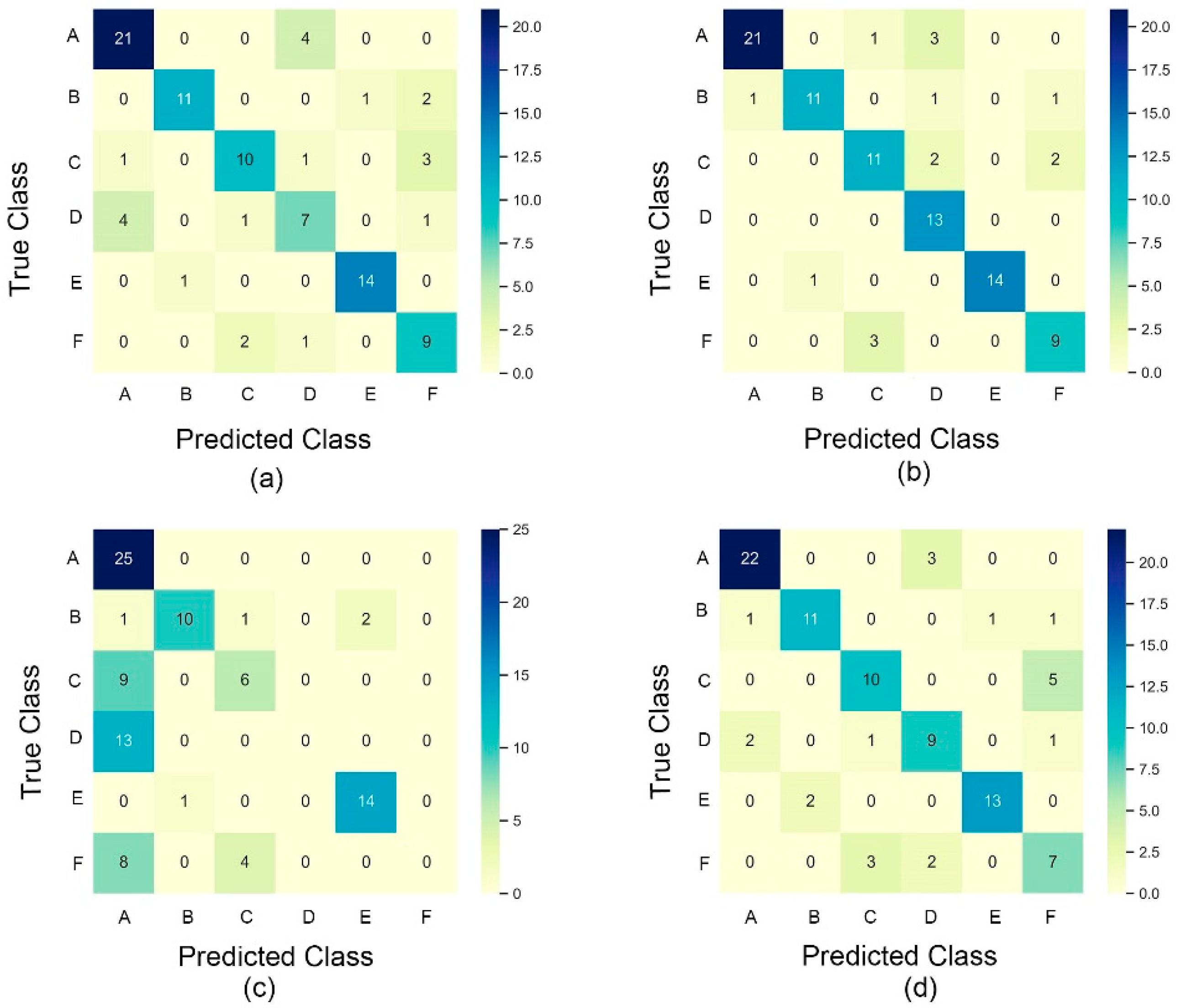
The results of the classification of each tree species are shown in Figure 7. It can be seen that the best overall classification result is provided by the BP neural network. SVM also achieved good classification results for some tree species, but the results for Acer negundo and Koelreuteria paniculate are poor. The SVM divided all 13 cases of Acer negundo into Fraxinus pennsylvanica and 12 cases of Koelreuteria paniculate into Fraxinus pennsylvanica and Robinia pseudoacacia.

Figure 7.
Classification results for different tree species using tree attributes. A, B, C, D, E, and F represent Fraxinus pennsylvanica, Ginkgo biloba, Robinia pseudoacacia, Acer negundo, Populus tomentosa, and Koelreuteria paniculate, respectively. (a) Random forest; (b) back propagation (BP) neural network; (c) support vector machine; and (d) K-nearest neighbor.
4.3. Results of the Classifciation Using Combined Attributes
The results of the four machine learning classification methods presented in Section 4.2 were used to classify the combined attributes of the trees, and the results are listed in Table 6. It can be seen that that the tree species classification precision for RF, BP neural network, and SVM using combined attributes is improved compared with that with classification based on a single tree attribute. The largest improvement is for SVM, with an improvement of 7.7%. However, the classification accuracy of KNN is 13.3% lower than when using a single tree attribute. The highest classification accuracy among the four methods is still provided by BP neural network, with a classification accuracy of 89.1%. Although the classification accuracy of SVM was increased, it is still the lowest among the four methods. From the perspective of different tree species, the best classification result is for Populus tomentosa, for which three classification methods had an accuracy of 100%, followed in order of decreasing accuracy by Ginkgo biloba, Fraxinus pennsylvanica, and Robinia pseudoacacia. The worst classification results are for Koelreuteria paniculate and Acer negundo, with a classification precision generally less than 80%. After combining the tree attributes, the classification precision for SVM for Koelreuteria paniculate and Acer negundo is still 0%, thus we conclude that the SVM method is not suitable for use as a tree species classifier based on the measured attributes.

Table 6.
Classification results using combined attributes.
The classification results for different tree species using each classification method with the combined attributes are illustrated in Figure 8. It can be seen that, compared with Figure 7, the classification results for all algorithms except for KNN have improved, and that the misclassification of each tree species is essentially the same as before.
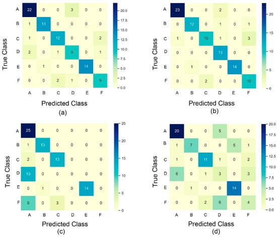
Figure 8.
Classification results for each tree species using combined attributes. A, B, C, D, E, and F represent Fraxinus pennsylvanica, Ginkgo biloba, Robinia pseudoacacia, Acer negundo, Populus tomentosa, and Koelreuteria paniculate, respectively. (a) Random forest; (b) BP neural network; (c) support vector machine; and (d) K-nearest neighbor.
5. Discussion
5.1. Analysis of the Acuarcy of Tree Attributes Extraction
We used image data obtained by optical drone tilt photogrammetry to establish a three-dimensional point cloud model of street trees using PIX4D software, and then automatically extracted individual tree attributes. From the perspective of the extraction accuracy of individual tree attributes, that for crown width is the highest, with an extraction accuracy close to 90% in both directions. The attribute with the worst extraction accuracy is tree height, with an accuracy of ~83%; this is because the measurement of tree height is easily affected by external environmental factors such as wind speed and human operator errors during field measurement. Another reason for the low accuracy of tree height estimation is that the tree point cloud model obtained by drone tilt photogrammetry modeling is blocked by branches and leaves, resulting in a sparse point cloud for the lower part of the tree, and the lowest point of the trunk cannot be accurately obtained when automatically calculating the tree height [47,50].
The results for tree attribute extraction reveal pronounced accuracy differences for different tree species, with the error of each extracted attribute for Fraxinus pennsylvanica being significantly larger than for the other species. There are several possible reasons for this, including the irregular crown shape, complex sample site environment, and numerous noise points. The extraction accuracies for tree height, crown height, and crown width all exceed 80%, and there is a good correlation between the calculated results and the true values. Although the results are lower than the extraction accuracy obtained using Lidar [50,51], we conclude that the attributes used in tree species classification in this study fulfill our requirements.
Canopy volume is also an important tree attribute and is being increasingly used to represent the three-dimensional greenness of urban trees [52,53]. The traditional method of calculating canopy volume only addresses the external crown shape and does not consider the space within the canopy [49,54]. The voxel method not only reflects the outer contour of the canopy, but also considers the voids within [48], and it is a good choice for accurately calculating the crown volume. However, because of the limitations of the experimental method, the true value cannot be measured; therefore, we did not consider the extraction accuracy of crown volume and we only analyzed the correlation between crown volume and the crown shape, with the correlation coefficient between the two canopy volume calculation methods being high (0.8417). Therefore, the crown volume calculated using the voxel method in this study reliably reflects the shape of the crown, which is an important attribute for the classification of tree species.
5.2. Analysis of the Accuracy of Tree Species Classification
In order to study the applicability of different methods of tree species classification, and to select appropriate classification methods based on tree attributes, four widely-used machine learning algorithms were selected. We found that the BP neural network classification algorithm had the best classification precision among the four classification methods. For individual tree attributes, the classification precision of the BP neural network algorithm reached 85.7%, and when combined attributes were used, the precision increased to 89.1%. The classification accuracy was higher than that obtained in other machine learning tree species classification studies [55,56], and the level attained met the requirements of the study. Among the four classification algorithms, the worst classification result was provided by SVM, with a classification precision using tree attributes of only 46.3%.
BP neural network is currently the most popular neural network model. It is a multi-layer feedforward neural network based on error back propagation, and it has strong nonlinear mapping capabilities and generalization capabilities [57]. Therefore, in its application to tree species classification, BP neural network has provided superior performance in nonlinear multi-classification problems compared with other machine learning algorithms. RF has a high prediction accuracy, has a good tolerance for outliers and noise, and is not prone to overfitting [58,59]. It is a widely used multi-class classifier and its performance in tree species classification is second only to the BP neural network. SVM is a linear classification method that can classify multi-dimensional data after adding a kernel function [60]. When the feature regions overlap significantly, the support vector machine is no longer applicable. Both KNN and SVM are simple machine learning classification algorithms [61]. Unlike SVM, KNN is more suitable for classification using large sample sizes, while the use of small sample sizes is more prone to misclassification. Different from other classification algorithms, after adding the combined features, the classification precision is lower than that using tree attributes. Overall, KNN is only suitable for simple classification, and the greater the number of classification attributes, the lower the classification precision.
From the perspective of the classification results of the SVM for different tree species, the results for Ginkgo biloba, Robinia pseudoacacia, and Populus tomentosa were of high quality; however, the classification precision for Koelreuteria paniculate and Acer negundo was 0%, which reduces its overall classification precision. The results of a principal component analysis (PCA) of individual tree attributes and combined attributes are illustrated in Figure 9; it can be seen that, for individual tree attributes, the distance between the attribute areas of each tree species is relatively low, and that the distance between the attribute areas increases after adding the combined attributes. This demonstrates that adding combined attributes can improve the classification precision of tree species. It can also be seen that the characteristic areas of Koelreuteria paniculate and Acer negundo mostly overlap, indicating that the characteristics of these two tree species are similar, and thus the precision of their classification.
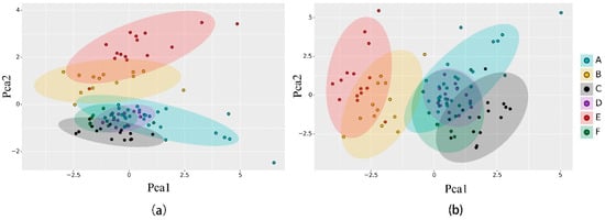
Figure 9.
Biplots of the results of principal components analysis of tree attributes. A, B, C, D, E, and F represent Fraxinus pennsylvanica, Ginkgo biloba, Robinia pseudoacacia, Acer negundo, Populus tomentosa, and Koelreuteria paniculate, respectively. (a) PCA (principal component analysis) results using individual attributes; (b) PCA results using combined attributes.
5.3. Limitations of the Study
Because of resource limitations, we only selected six representative tree species for study, and as the number of tree species increases, the classification results may change. Nevertheless, our results can serve as a pilot study for a large-scale urban street tree classification study in the future. In future research, the number of samples will be increased, and different seasons and different tree ages will be considered. Although multiple tree species were generally classified successfully, the classification results were less reliable for species such as Koelreuteria paniculate and Acer negundo, which have similar attributes. Moreover, the accuracy of tree species classification achieved in this study is still lower than for existing classification methods [28,29,30]; therefore, improving the classification precision for individual tree species will be the focus of future research. Finally, the superiority of the BP neural network for tree species classification and in other applications [62,63,64] points to a promising research direction of tree species classification algorithms in the future.
6. Conclusions
Our results demonstrate the feasibility of using tree attributes extracted by optical drone tilt photogrammetry to classify tree species. Compared with traditional methods, this approach has the advantages of automation, efficiency, and economy in terms of manpower and cost. The extraction results of tree attributes revealed that the relative error for tree height was the largest compared with the true value, followed by crown height and crown width. From the perspective of different tree species, the relative error of each attribute for Fraxinus pennsylvanica was the largest, and those for Koelreuteria paniculate, Acer negundo, and Robinia pseudoacacia were small. In terms of the strength of correlation between tree attributes and their optimal values, that for crown volume was the highest and that for tree height was the lowest.
In the automated extraction of tree attributes, different tree species can be accurately identified based on both individual attributes and combined attributes, with the results based on combined attributes being superior. In addition, the use of combined attributes for tree species classification was more accurate than the use of individual attributes. Among the four classification algorithms, the best classification result was provided by BP neural network, followed by RF, while the classification results using SVM and KNN were poor. The best classification results were provided by BP neural network using combined attributes.
Author Contributions
Conceptualization, Y.W. and J.W.; methodology, Y.W.; software, Y.W. and L.A.; validation, Y.W., L.A., Y.C., and J.X.; formal analysis, Y.W., S.C., and L.S.; investigation, Y.W., L.A., Y.C., J.X., S.C., and L.S.; resources, J.W.; data curation, Y.W.; writing—original draft preparation, Y.W.; writing—review and editing, Y.W. and J.W.; visualization, Y.W.; supervision, J.W.; project administration, Y.W.; funding acquisition, J.W. All authors have read and agreed to the published version of the manuscript.
Funding
This research was funded by the Fundamental Research Funds for the Natural Science Foundation of China (42071342, 31870713), the Beijing Natural Science Foundation Program (8182038), and the Fundamental Research Funds for the Central Universities (2015ZCQ-LX-01,2018ZY06).
Institutional Review Board Statement
Not applicable.
Informed Consent Statement
Not applicable.
Data Availability Statement
The data presented in this study are available in the supplementary material.
Acknowledgments
We are grateful to the undergraduate students and staff of the Laboratory of Forest Management and “3S” technology, Beijing Forestry University.
Conflicts of Interest
The authors declare no conflict of interest.
References
- Vennemo, H.; Aunan, K.; Lindhjem, H.; Seip, H.M. Environmental Pollution in China: Status and Trends; Oxford University Press: Oxford, UK, 2009. [Google Scholar]
- Gong, P.; Liang, S.; Carlton, E.J.; Jiang, Q.; Wu, J.; Wang, L.; Remais, J.V. Urbanisation and health in China. Lancet 2012, 379, 843–852. [Google Scholar] [CrossRef]
- Shrestha, R.; Flacke, J.; Martinez, J.; Van Maarseveen, M. Environmental health related socio-spatial inequalities: Identifying “hotspots” of environmental burdens and social vulnerability. Int. J. Environ. Res. Public Health 2016, 13, 691. [Google Scholar] [CrossRef]
- Wang, Y.; Akbari, H. The effects of street tree planting on Urban Heat Island mitigation in Montreal. Sustain. Cities Soc. 2016, 27, 122–128. [Google Scholar] [CrossRef]
- Sanders, R.A. Urban vegetation impacts on the hydrology of Dayton, Ohio. Urban Ecol. 1986, 9, 361–376. [Google Scholar] [CrossRef]
- Seamans, G.S. Mainstreaming the environmental benefits of street trees. Urban For. Urban Green. 2013, 12, 2–11. [Google Scholar] [CrossRef]
- Zhang, K.; Hu, B. Individual urban tree species classification using very high spatial resolution airborne multi-spectral imagery using longitudinal profiles. Remote Sens. 2012, 4, 1741–1757. [Google Scholar] [CrossRef]
- Thaiutsa, B.; Puangchit, L.; Kjelgren, R.; Arunpraparut, W. Urban green space, street tree and heritage large tree assessment in Bangkok, Thailand. Urban For. Urban Green. 2008, 7, 219–229. [Google Scholar] [CrossRef]
- Dinuls, R.; Erins, G.; Lorencs, A.; Mednieks, I.; Sinica-Sinavskis, J. Tree species identification in mixed Baltic forest using LiDAR and multispectral data. IEEE J. Sel. Top. Appl. Earth Obs. Remote Sens. 2012, 5, 594–603. [Google Scholar] [CrossRef]
- Yahiaoui, I.; Mzoughi, O.; Boujemaa, N. Leaf shape descriptor for tree species identification. In Proceedings of the 2012 IEEE International Conference on Multimedia and Expo, Melbourne, VIC, Australia, 9–13 July 2012; pp. 254–259. [Google Scholar]
- Meyera, P.; Staenzb, K.; Ittena, K. Semi-automated procedures for tree species identification in high spatial resolution data from digitized colour infrared-aerial photography. ISPRS J. Photogramm. Remote Sens. 1996, 51, 5–16. [Google Scholar] [CrossRef]
- Kim, S.; Schreuder, G.; McGaughey, R.J.; Andersen, H.-E. Individual tree species identification using LIDAR intensity data. In Proceedings of the ASPRS 2008 Annual Conference, Portland, OR, USA, 28 April–2 May 2008. [Google Scholar]
- Korpela, I.; Mehtätalo, L.; Markelin, L.; Seppänen, A.; Kangas, A. Tree species identification in aerial image data using directional reflectance signatures. Silva Fenn. 2014, 48, 1087. [Google Scholar] [CrossRef]
- Agarwal, S.; Vailshery, L.S.; Jaganmohan, M.; Nagendra, H. Mapping urban tree species using very high resolution satellite imagery: Comparing pixel-based and object-based approaches. ISPRS Int. J. Geo-Inf. 2013, 2, 220–236. [Google Scholar] [CrossRef]
- Effiom, A.E.; van Leeuwen, L.M.; Nyktas, P.; Okojie, J.A.; Erdbrügger, J. Combining unmanned aerial vehicle and multispectral Pleiades data for tree species identification, a prerequisite for accurate carbon estimation. J. Appl. Remote Sens. 2019, 13, 034530. [Google Scholar] [CrossRef]
- Maschler, J.; Atzberger, C.; Immitzer, M. Individual tree crown segmentation and classification of 13 tree species using airborne hyperspectral data. Remote Sens. 2018, 10, 1218. [Google Scholar] [CrossRef]
- Korpela, I.; Tokola, T.; Ørka, H.; Koskinen, M. Small-footprint discrete-return LiDAR in tree species recognition. In Proceedings of the ISPRS Hannover Workshop 2009, Hannover, Germany, 2–5 June 2009; pp. 1–6. [Google Scholar]
- Korpela, I.; Dahlin, B.; Schäfer, H.; Bruun, E.; Haapaniemi, F.; Honkasalo, J.; Ilvesniemi, S.; Kuutti, V.; Linkosalmi, M.; Mustonen, J. Single-tree forest inventory using lidar and aerial images for 3D treetop positioning, species recognition, height and crown width estimation. In Proceedings of the ISPRS Workshop on Laser Scanning, Espoo, Finland, 12–14 September 2007; pp. 227–233. [Google Scholar]
- Haala, N.; Reulke, R.; Thies, M.; Aschoff, T. Combination of terrestrial laser scanning with high resolution panoramic images for investigations in forest applications and tree species recognition. In Proceedings of the ISPRS Working Group V/1, Dresden, Germany, 19–22 February 2004. [Google Scholar]
- Zhang, C.; Qiu, F. Mapping individual tree species in an urban forest using airborne lidar data and hyperspectral imagery. Photogramm. Eng. Remote Sens. 2012, 78, 1079–1087. [Google Scholar] [CrossRef]
- Liu, L.; Coops, N.C.; Aven, N.W.; Pang, Y. Mapping urban tree species using integrated airborne hyperspectral and LiDAR remote sensing data. Remote Sens. Environ. 2017, 200, 170–182. [Google Scholar] [CrossRef]
- Shi, Y.; Skidmore, A.K.; Wang, T.; Holzwarth, S.; Heiden, U.; Pinnel, N.; Zhu, X.; Heurich, M. Tree species classification using plant functional traits from LiDAR and hyperspectral data. Int. J. Appl. Earth Obs. Geoinf. 2018, 73, 207–219. [Google Scholar] [CrossRef]
- Åkerblom, M.; Raumonen, P.; Mäkipää, R.; Kaasalainen, M. Automatic tree species recognition with quantitative structure models. Remote Sens. Environ. 2017, 191, 1–12. [Google Scholar] [CrossRef]
- Raczko, E.; Zagajewski, B. Comparison of support vector machine, random forest and neural network classifiers for tree species classification on airborne hyperspectral APEX images. Eur. J. Remote Sens. 2017, 50, 144–154. [Google Scholar] [CrossRef]
- Franklin, S.E.; Ahmed, O.S. Deciduous tree species classification using object-based analysis and machine learning with unmanned aerial vehicle multispectral data. Int. J. Remote Sens. 2018, 39, 5236–5245. [Google Scholar] [CrossRef]
- Vauhkonen, J.; Ørka, H.O.; Holmgren, J.; Dalponte, M.; Heinzel, J.; Koch, B. Tree species recognition based on airborne laser scanning and complementary data sources. In Forestry Applications of Airborne Laser Scanning; Springer: Berlin/Heidelberg, Germany, 2014; pp. 135–156. [Google Scholar]
- Othmani, A.; Voon, L.F.L.Y.; Stolz, C.; Piboule, A. Single tree species classification from terrestrial laser scanning data for forest inventory. Pattern Recognit. Lett. 2013, 34, 2144–2150. [Google Scholar] [CrossRef]
- Zhang, B.; Zhao, L.; Zhang, X. Three-dimensional convolutional neural network model for tree species classification using airborne hyperspectral images. Remote Sens. Environ. 2020, 247, 111938. [Google Scholar] [CrossRef]
- Zhang, H.; He, G.; Peng, J.; Kuang, Z.; Fan, J. Deep learning of path-based tree classifiers for large-scale plant species identification. In Proceedings of the 2018 IEEE Conference on Multimedia Information Processing and Retrieval (MIPR), Miami, FL, USA, 10–12 April 2018; pp. 25–30. [Google Scholar]
- Xi, Z.; Hopkinson, C.; Rood, S.B.; Peddle, D.R. See the forest and the trees: Effective machine and deep learning algorithms for wood filtering and tree species classification from terrestrial laser scanning. ISPRS J. Photogramm. Remote Sens. 2020, 168, 1–16. [Google Scholar] [CrossRef]
- Qi, C.R.; Yi, L.; Su, H.; Guibas, L.J. Pointnet++: Deep hierarchical feature learning on point sets in a metric space. In Proceedings of the Advances in Neural Information Processing Systems 30 Confernce(NIPS 2017), Long Beach, CA, USA, 4–6 December 2017; pp. 5099–5108. [Google Scholar]
- Berteška, T.; Gečyte, S.; Jakubauskienė, E.; Aksamitauskas, V.Č. The surface modelling based on UAV Photogrammetry and qualitative estimation. Measurement 2015, 73, 619–627. [Google Scholar]
- Huang, C.; Zhang, H.; Zhao, J. High-Efficiency Determination of Coastline by Combination of Tidal Level and Coastal Zone DEM from UAV Tilt Photogrammetry. Remote Sens. 2020, 12, 2189. [Google Scholar] [CrossRef]
- Ren, J.; Chen, X.; Zheng, Z. Future Prospects of UAV Tilt Photogrammetry Technology. IOP Conf. Ser. Mater. Sci. Eng. 2019, 612, 032023. [Google Scholar] [CrossRef]
- Olli, N.; Eija, H.; Sakari, T.; Niko, V.; Teemu, H.; Xiaowei, Y.; Juha, H.; Heikki, S.; Ilkka, P.L.N.; Nilton, I. Individual Tree Detection and Classification with UAV-Based Photogrammetric Point Clouds and Hyperspectral Imaging. Remote Sens. 2017, 9, 185. [Google Scholar]
- Berteška, T.; Ruzgien, B. Photogrammetric mapping based on UAV imagery. Geod. Cartogr. 2013, 39, 158–163. [Google Scholar] [CrossRef]
- Yang, B.; Luhe, W.; University, H.N. Model of Building 3D Model Based on UAV Incline Photogrammetry. Nat. Ence J. Harbin Norm. Univ. 2017, 33, 81–86. [Google Scholar]
- Torresan, C.; Berton, A.; Carotenuto, F.; Di Gennaro, S.F.; Gioli, B.; Matese, A.; Miglietta, F.; Vagnoli, C.; Zaldei, A.; Wallace, L. Forestry applications of UAVs in Europe: A review. Int. J. Remote Sens. 2017, 38, 2427–2447. [Google Scholar] [CrossRef]
- Park, S.; Yun, S.; Kim, H.; Kwon, R.; Ganser, J.; Anthony, S. Forestry monitoring system using lora and drone. In Proceedings of the 8th International Conference on Web Intelligence, Mining and Semantics, Novi Sad, Serbia, 25–27 June 2018; pp. 1–8. [Google Scholar]
- Tang, L.; Shao, G. Drone remote sensing for forestry research and practices. J. For. Res. 2015, 26, 791–797. [Google Scholar] [CrossRef]
- Cao, L.; Liu, H.; Fu, X.; Zhang, Z.; Shen, X.; Ruan, H. Comparison of UAV LiDAR and digital aerial photogrammetry point clouds for estimating forest structural attributes in subtropical planted forests. Forests 2019, 10, 145. [Google Scholar] [CrossRef]
- Qiu, Z.; Feng, Z.-K.; Wang, M.; Li, Z.; Lu, C. Application of UAV photogrammetric system for monitoring ancient tree communities in Beijing. Forests 2018, 9, 735. [Google Scholar] [CrossRef]
- Taddia, Y.; Stecchi, F.; Pellegrinelli, A. Coastal Mapping using DJI Phantom 4 RTK in Post-Processing Kinematic Mode. Drones 2020, 4, 9. [Google Scholar] [CrossRef]
- Rusu, R.B.; Marton, Z.C.; Blodow, N.; Dolha, M.; Beetz, M. Towards 3D point cloud based object maps for household environments. Robot. Auton. Syst. 2008, 56, 927–941. [Google Scholar] [CrossRef]
- Tao, S.; Guo, Q.; Xu, S.; Su, Y.; Li, Y.; Wu, F. A geometric method for wood-leaf separation using terrestrial and simulated lidar data. Photogramm. Eng. Remote Sens. 2015, 81, 767–776. [Google Scholar] [CrossRef]
- Moskal, L.M.; Zheng, G. Retrieving forest inventory variables with terrestrial laser scanning (TLS) in urban heterogeneous forest. Remote Sens. 2012, 4, 1–20. [Google Scholar] [CrossRef]
- Tian, J.; Dai, T.; Li, H.; Liao, C.; Teng, W.; Hu, Q.; Ma, W.; Xu, Y. A novel tree height extraction approach for individual trees by combining TLS and UAV image-based point cloud integration. Forests 2019, 10, 537. [Google Scholar] [CrossRef]
- Kükenbrink, D.; Schneider, F.D.; Leiterer, R.; Schaepman, M.E.; Morsdorf, F. Quantification of hidden canopy volume of airborne laser scanning data using a voxel traversal algorithm. Remote Sens. Environ. 2017, 194, 424–436. [Google Scholar] [CrossRef]
- Nelson, R. Modeling forest canopy heights: The effects of canopy shape. Remote Sens. Environ. 1997, 60, 327–334. [Google Scholar] [CrossRef]
- Andersen, H.-E.; Reutebuch, S.E.; McGaughey, R.J. A rigorous assessment of tree height measurements obtained using airborne lidar and conventional field methods. Can. J. Remote Sens. 2006, 32, 355–366. [Google Scholar] [CrossRef]
- Liu, H.; Wu, C. Tree Crown width estimation, using discrete airborne LiDAR data. Can. J. Remote Sens. 2016, 42, 610–618. [Google Scholar] [CrossRef]
- LaRue, E.A.; Atkins, J.W.; Dahlin, K.; Fahey, R.; Fei, S.; Gough, C.; Hardiman, B.S. Linking Landsat to terrestrial LiDAR: Vegetation metrics of forest greenness are correlated with canopy structural complexity. Int. J. Appl. Earth Obs. Geoinf. 2018, 73, 420–427. [Google Scholar] [CrossRef]
- Van Leeuwen, M.; Coops, N.C.; Wulder, M.A. Canopy surface reconstruction from a LiDAR point cloud using Hough transform. Remote Sens. Lett. 2010, 1, 125–132. [Google Scholar] [CrossRef]
- Thorne, M.S.; Skinner, Q.D.; Smith, M.A.; Rodgers, J.D.; Laycock, W.A.; Cerekci, S.A. Evaluation of a technique for measuring canopy volume of shrubs. Rangel. Ecol. Manag./J. Range Manag. Arch. 2002, 55, 235–241. [Google Scholar] [CrossRef]
- Ko, C.; Sohn, G.; Remmel, T.K. Tree genera classification with geometric features from high-density airborne LiDAR. Can. J. Remote Sens. 2013, 39, S73–S85. [Google Scholar] [CrossRef]
- Li, J.; Hu, B.; Noland, T.L. Classification of tree species based on structural features derived from high density LiDAR data. Agric. For. Meteorol. 2013, 171, 104–114. [Google Scholar] [CrossRef]
- Li, J.; Cheng, J.-H.; Shi, J.-Y.; Huang, F. Brief introduction of back propagation (BP) neural network algorithm and its improvement. In Advances in Computer Science and Information Engineering; Springer: Berlin/Heidelberg, Germany, 2012; pp. 553–558. [Google Scholar]
- Qi, Y. Random forest for bioinformatics. In Ensemble Machine Learning; Springer: Berlin/Heidelberg, Germany, 2012; pp. 307–323. [Google Scholar]
- Rodriguez-Galiano, V.F.; Ghimire, B.; Rogan, J.; Chica-Olmo, M.; Rigol-Sanchez, J.P. An assessment of the effectiveness of a random forest classifier for land-cover classification. ISPRS J. Photogramm. Remote Sens. 2012, 67, 93–104. [Google Scholar] [CrossRef]
- Hearst, M.A.; Dumais, S.T.; Osuna, E.; Platt, J.; Scholkopf, B. Support vector machines. IEEE Intell. Syst. Their Appl. 1998, 13, 18–28. [Google Scholar] [CrossRef]
- Zhang, H.; Berg, A.C.; Maire, M.; Malik, J. SVM-KNN: Discriminative nearest neighbor classification for visual category recognition. In Proceedings of the 2006 IEEE Computer Society Conference on Computer Vision and Pattern Recognition (CVPR’06), New York, NY, USA, 17–22 June 2006; pp. 2126–2136. [Google Scholar]
- Wang, B.; Gu, X.; Ma, L.; Yan, S. Temperature error correction based on BP neural network in meteorological wireless sensor network. Int. J. Sens. Netw. 2017, 23, 265–278. [Google Scholar] [CrossRef]
- Li, D.-J.; Li, Y.-Y.; Li, J.-X.; Fu, Y. Gesture recognition based on BP neural network improved by chaotic genetic algorithm. Int. J. Autom. Comput. 2018, 15, 267–276. [Google Scholar] [CrossRef]
- Ma, D.; Zhou, T.; Chen, J.; Qi, S.; Shahzad, M.A.; Xiao, Z. Supercritical water heat transfer coefficient prediction analysis based on BP neural network. Nucl. Eng. Des. 2017, 320, 400–408. [Google Scholar] [CrossRef]
Publisher’s Note: MDPI stays neutral with regard to jurisdictional claims in published maps and institutional affiliations. |
© 2021 by the authors. Licensee MDPI, Basel, Switzerland. This article is an open access article distributed under the terms and conditions of the Creative Commons Attribution (CC BY) license (http://creativecommons.org/licenses/by/4.0/).

