A Novel Method for Automated Supraglacial Lake Mapping in Antarctica Using Sentinel-1 SAR Imagery and Deep Learning


Abstract
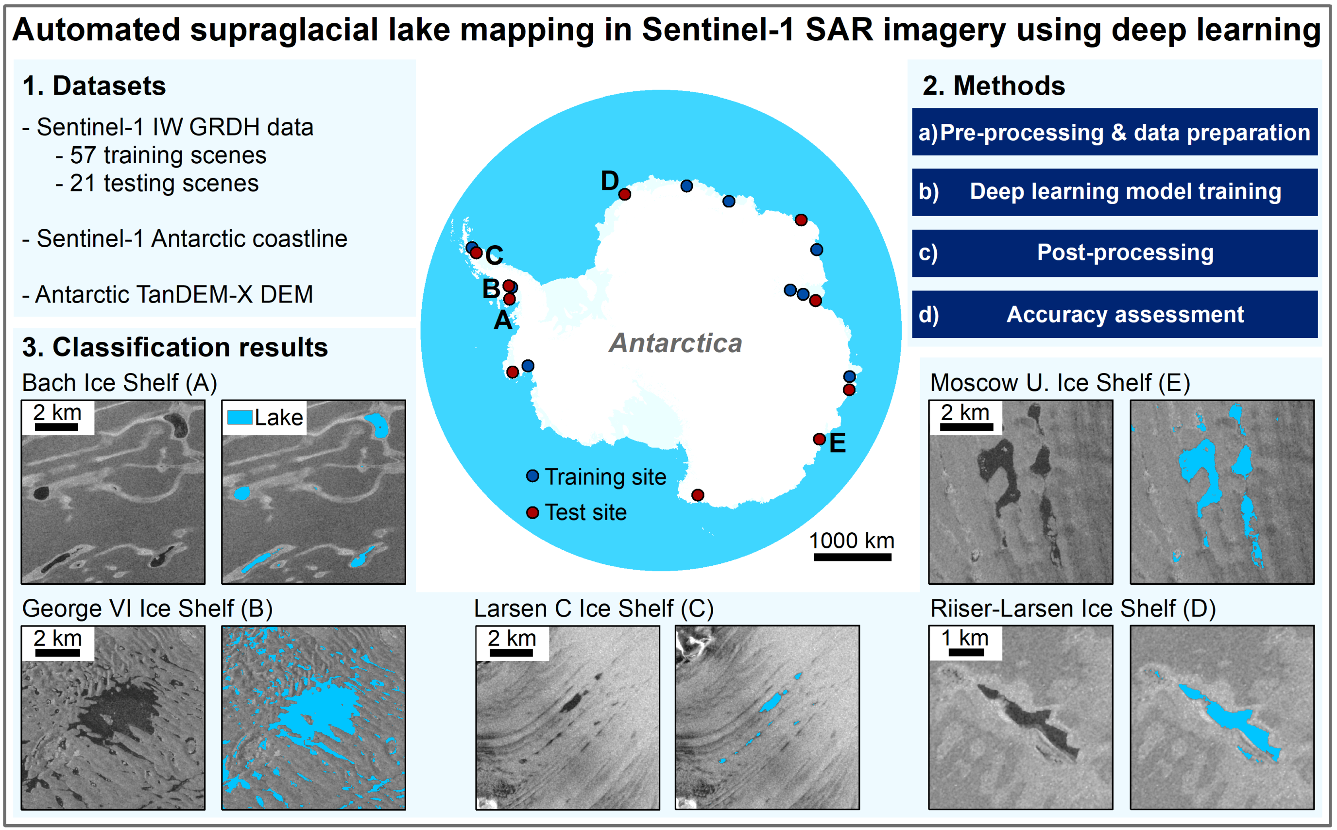
1. Introduction
2. Materials and Methods
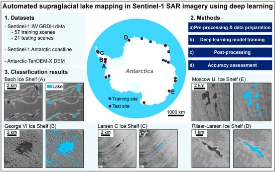
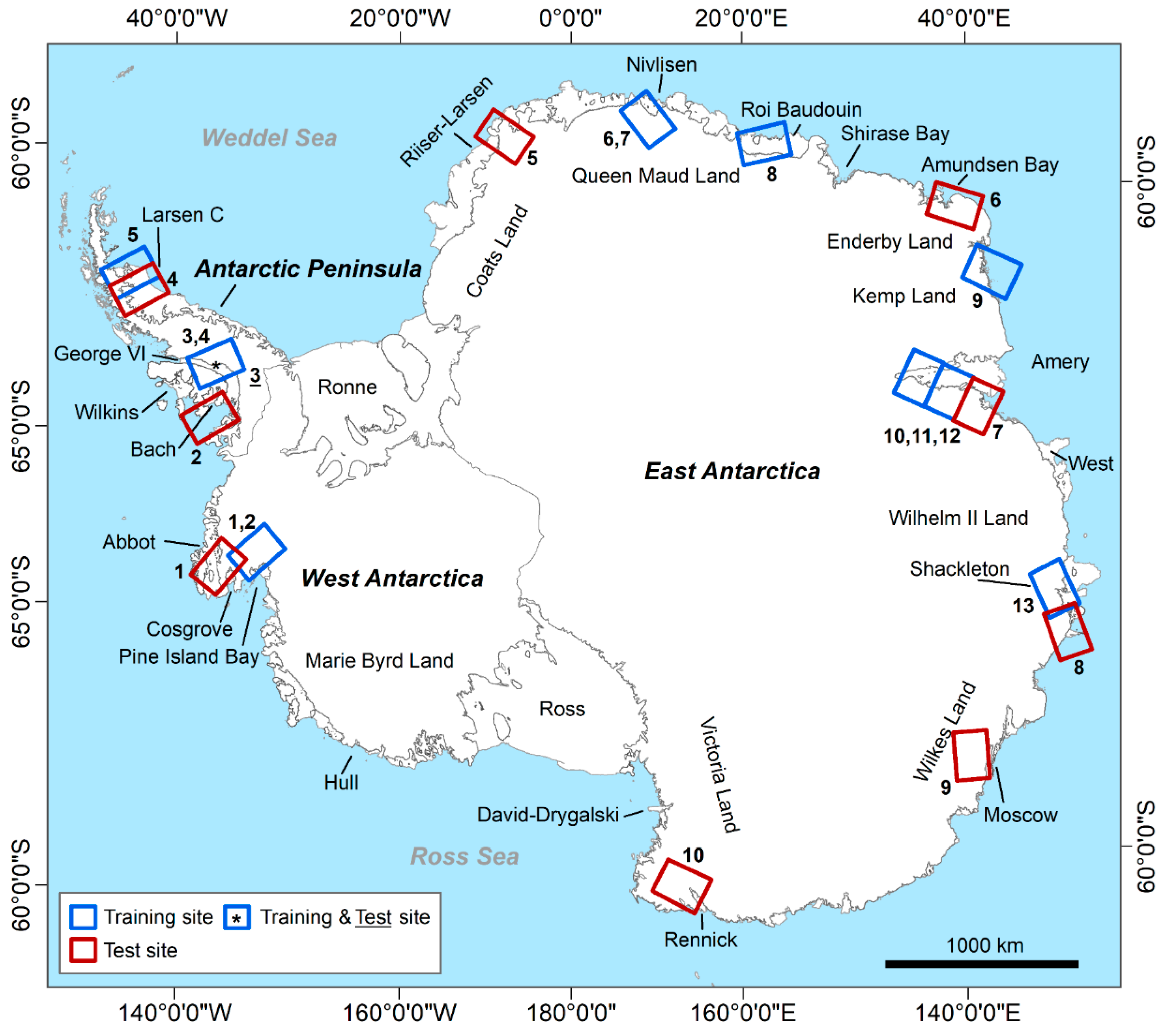
2.1. Study Sites
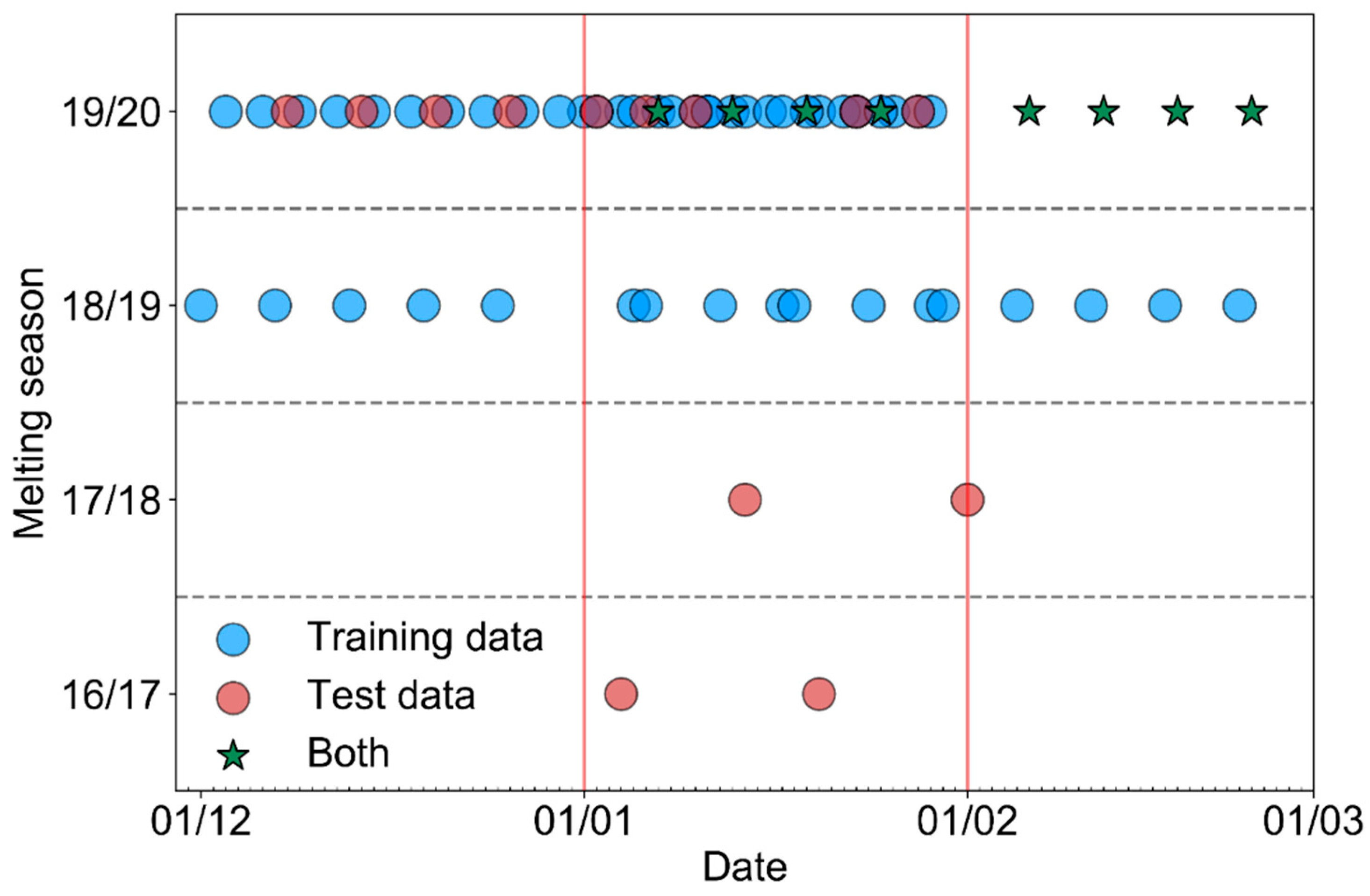
2.2. Datasets
2.2.1. Sentinel-1 Data
2.2.2. Topographic Data
2.2.3. Coastline Data
2.3. Methods
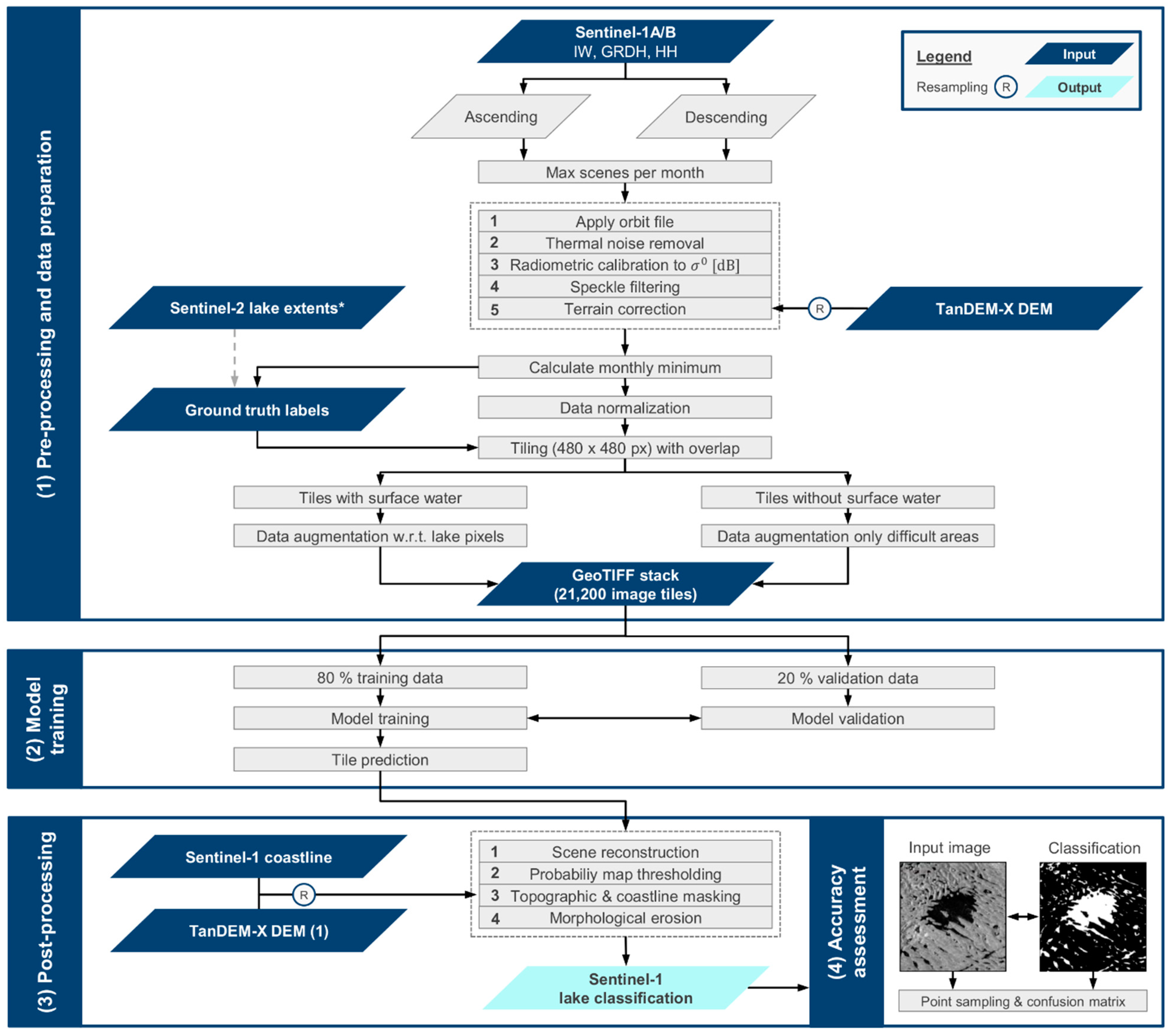
2.3.1. Pre-Processing and Data Preparation
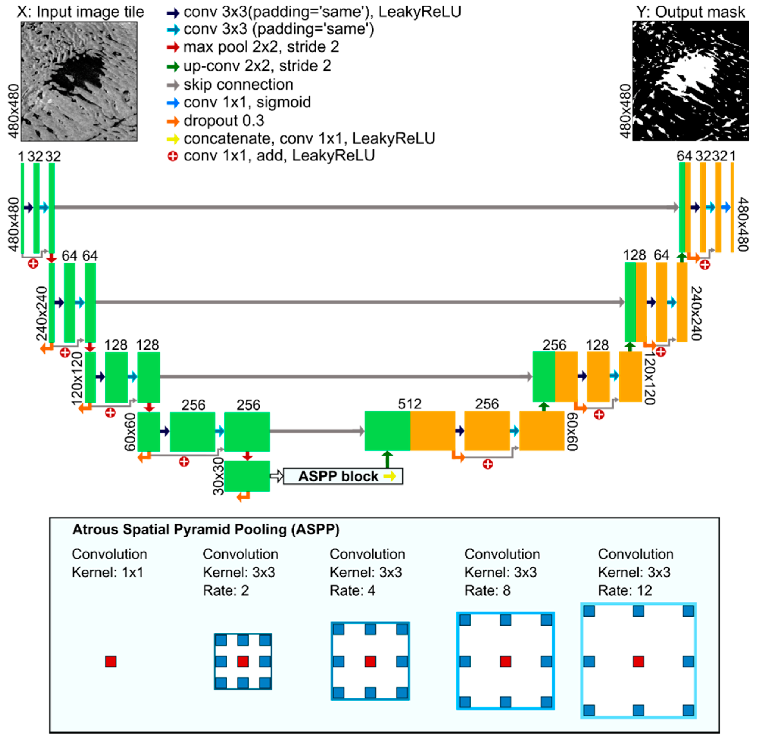
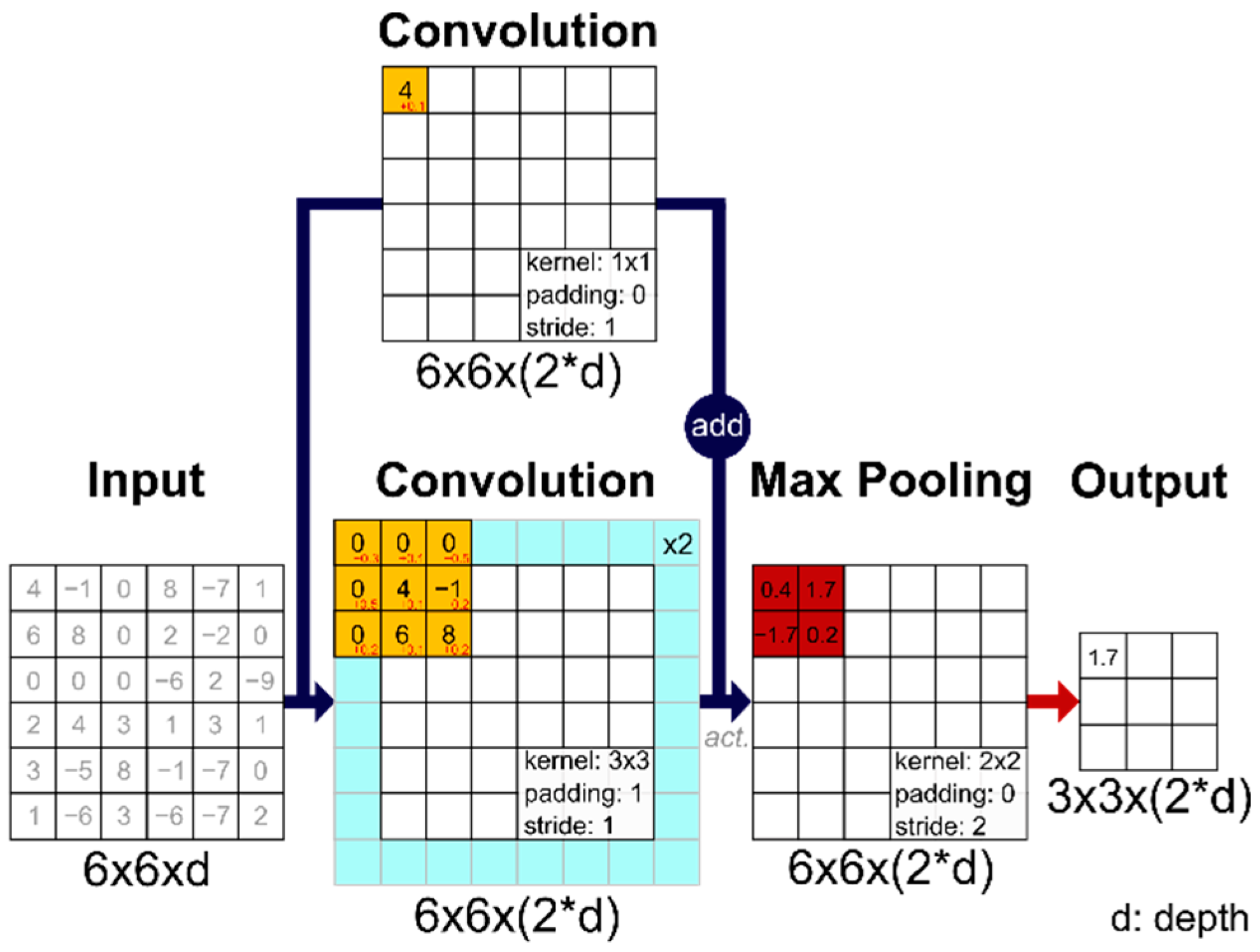
2.3.2. Deep Learning Model Training
2.3.3. Post-Processing
2.3.4. Accuracy Assessment
3. Results
3.1. Classification Results
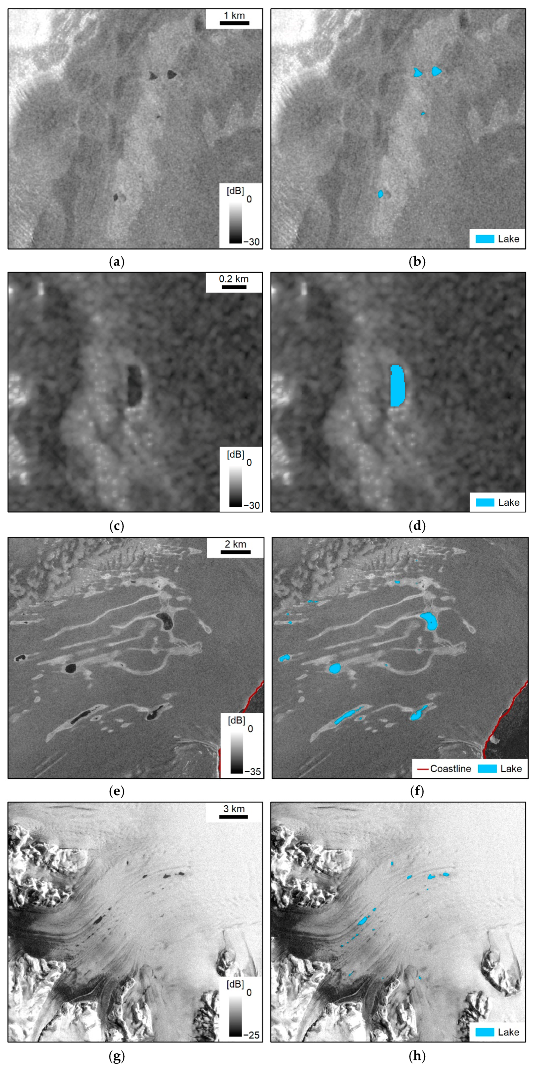
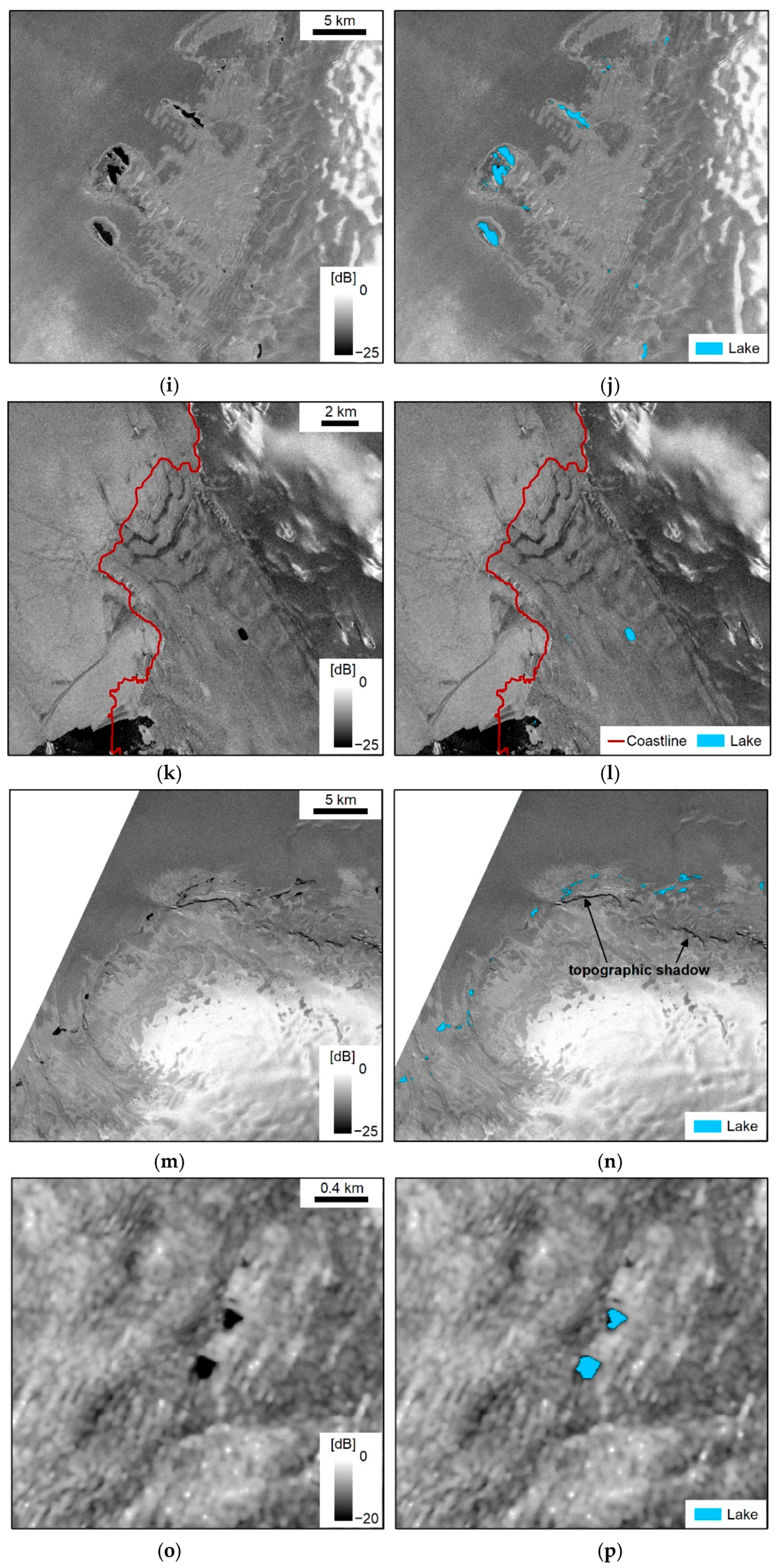
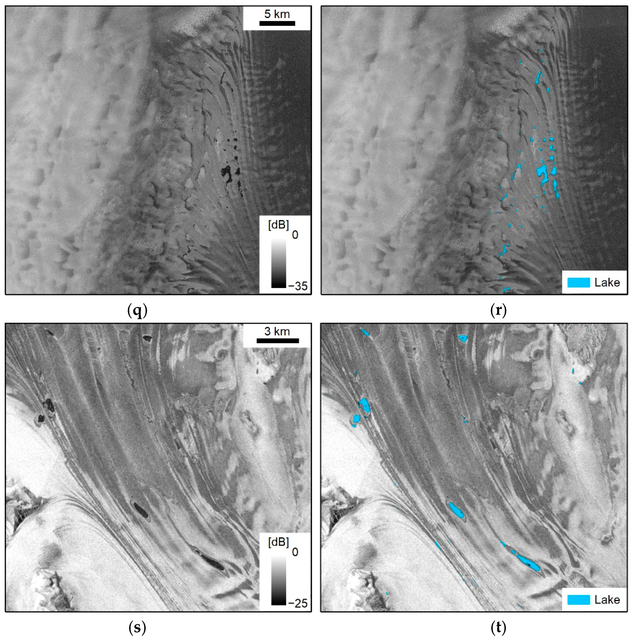
3.1.1. Test Regions
3.1.2. Spatio-Temporal Lake Dynamics on George VI Ice Shelf
3.2. Accuracy Assessment
4. Discussion
4.1. Classification Results
4.2. Accuracy Assessment
4.3. Future Requirements
5. Conclusions
Supplementary Materials
Author Contributions
Funding
Institutional Review Board Statement
Informed Consent Statement
Data Availability Statement
Acknowledgments
Conflicts of Interest
References
- Shepherd, A.; Ivins, E.; Rignot, E.; Smith, B.; van Den Broeke, M.; Velicogna, I.; Whitehouse, P.; Briggs, K.; Joughin, I.; Krinner, G.; et al. Mass Balance of the Greenland Ice Sheet from 1992 to 2018. Nature 2020, 579, 233–239. [Google Scholar] [CrossRef]
- Shepherd, A.; Ivins, E.; Rignot, E.; Smith, B.; Van den Broeke, M.; Velicogna, I.; Whitehouse, P.; Briggs, K.; Joughin, I.; Krinner, G.; et al. Mass Balance of the Antarctic Ice Sheet from 1992 to 2017. Nature 2018, 558, 219–222. [Google Scholar] [CrossRef]
- Enderlin, E.M.; Howat, I.M.; Jeong, S.; Noh, M.-J.; van Angelen, J.H.; van den Broeke, M.R. An Improved Mass Budget for the Greenland Ice Sheet. Geophys. Res. Lett. 2014, 41, 866–872. [Google Scholar] [CrossRef]
- Mouginot, J.; Rignot, E.; Bjørk, A.A.; van den Broeke, M.; Millan, R.; Morlighem, M.; Noël, B.; Scheuchl, B.; Wood, M. Forty-Six Years of Greenland Ice Sheet Mass Balance from 1972 to 2018. Proc. Natl. Acad. Sci. USA 2019, 116, 9239–9244. [Google Scholar] [CrossRef] [PubMed]
- Bell, R.E.; Banwell, A.F.; Trusel, L.D.; Kingslake, J. Antarctic Surface Hydrology and Impacts on Ice-Sheet Mass Balance. Nat. Clim. Chang. 2018, 8, 1044. [Google Scholar] [CrossRef]
- Das, S.B.; Joughin, I.; Behn, M.D.; Howat, I.M.; King, M.A.; Lizarralde, D.; Bhatia, M.P. Fracture Propagation to the Base of the Greenland Ice Sheet During Supraglacial Lake Drainage. Science 2008, 320, 778–781. [Google Scholar] [CrossRef]
- Shepherd, A.; Hubbard, A.; Nienow, P.; King, M.; McMillan, M.; Joughin, I. Greenland Ice Sheet Motion Coupled with Daily Melting in Late Summer. Geophys. Res. Lett. 2009, 36. [Google Scholar] [CrossRef]
- Tedesco, M.; Willis, I.C.; Hoffman, M.J.; Banwell, A.F.; Alexander, P.; Arnold, N.S. Ice Dynamic Response to Two Modes of Surface Lake Drainage on the Greenland Ice Sheet. Environ. Res. Lett. 2013, 8, 034007. [Google Scholar] [CrossRef]
- Zwally, H.J.; Abdalati, W.; Herring, T.; Larson, K.; Saba, J.; Steffen, K. Surface Melt-Induced Acceleration of Greenland Ice-Sheet Flow. Science 2002, 297, 218–222. [Google Scholar] [CrossRef]
- Bartholomew, I.; Nienow, P.; Mair, D.; Hubbard, A.; King, M.A.; Sole, A. Seasonal Evolution of Subglacial Drainage and Acceleration in a Greenland Outlet Glacier. Nat. Geosci. 2010, 3, 408–411. [Google Scholar] [CrossRef]
- Banwell, A.F.; Macayeal, D.R. Ice-Shelf Fracture Due to Viscoelastic Flexure Stress Induced by Fill/Drain Cycles of Supraglacial Lakes. Antarct. Sci. 2015, 27, 587–597. [Google Scholar] [CrossRef]
- Banwell, A.F.; MacAyeal, D.R.; Sergienko, O.V. Breakup of the Larsen B Ice Shelf Triggered by Chain Reaction Drainage of Supraglacial Lakes. Geophys. Res. Lett. 2013, 40, 5872–5876. [Google Scholar] [CrossRef]
- Rignot, E.; Casassa, G.; Gogineni, P.; Krabill, W.; Rivera, A.; Thomas, R. Accelerated Ice Discharge from the Antarctic Peninsula Following the Collapse of Larsen B Ice Shelf. Geophys. Res. Lett. 2004, 31. [Google Scholar] [CrossRef]
- Rott, H.; Abdel Jaber, W.; Wuite, J.; Scheiblauer, S.; Floricioiu, D.; Van Wessem, J.M.; Nagler, T.; Miranda, N.; Van den Broeke, M.R. Changing Pattern of Ice Flow and Mass Balance for Glaciers Discharging into the Larsen A and B Embayments, Antarctic Peninsula, 2011 to 2016. Cryosphere 2018, 12, 1273–1291. [Google Scholar] [CrossRef]
- Scambos, T.A.; Bohlander, J.A.; Shuman, C.A.; Skvarca, P. Glacier Acceleration and Thinning after Ice Shelf Collapse in the Larsen B Embayment, Antarctica. Geophys. Res. Lett. 2004, 31. [Google Scholar] [CrossRef]
- Tedesco, M.; Lüthje, M.; Steffen, K.; Steiner, N.; Fettweis, X.; Willis, I.; Bayou, N.; Banwell, A. Measurement and Modeling of Ablation of the Bottom of Supraglacial Lakes in Western Greenland. Geophys. Res. Lett. 2012, 39. [Google Scholar] [CrossRef]
- Lüthje, M.; Pedersen, L.T.; Reeh, N.; Greuell, W. Modelling the Evolution of Supraglacial Lakes on the West Greenland Ice-Sheet Margin. J. Glaciol. 2006, 52, 608–618. [Google Scholar] [CrossRef]
- Stokes, C.R.; Sanderson, J.E.; Miles, B.W.J.; Jamieson, S.S.R.; Leeson, A.A. Widespread Distribution of Supraglacial Lakes around the Margin of the East Antarctic Ice Sheet. Sci. Rep. 2019, 9, 13823. [Google Scholar] [CrossRef]
- Kingslake, J.; Ely, J.C.; Das, I.; Bell, R.E. Widespread Movement of Meltwater onto and across Antarctic Ice Shelves. Nature 2017, 544, 349–352. [Google Scholar] [CrossRef]
- Tuckett, P.A.; Ely, J.C.; Sole, A.J.; Livingstone, S.J.; Davison, B.J.; van Wessem, J.M.; Howard, J. Rapid Accelerations of Antarctic Peninsula Outlet Glaciers Driven by Surface Melt. Nat. Commun. 2019, 10, 1–8. [Google Scholar] [CrossRef]
- Langley, E.S.; Leeson, A.A.; Stokes, C.R.; Jamieson, S.S.R. Seasonal Evolution of Supraglacial Lakes on an East Antarctic Outlet Glacier. Geophys. Res. Lett. 2016, 43, 8563–8571. [Google Scholar] [CrossRef]
- Leeson, A.A.; Forster, E.; Rice, A.; Gourmelen, N.; Van Wessem, J.M. Evolution of Supraglacial Lakes on the Larsen B Ice Shelf in the Decades before It Collapsed. Geophys. Res. Lett. 2020, 47. [Google Scholar] [CrossRef]
- Arthur, J.F.; Stokes, C.R.; Jamieson, S.S.R.; Carr, J.R.; Leeson, A.A. Distribution and Seasonal Evolution of Supraglacial Lakes on Shackleton Ice Shelf, East Antarctica. Cryosphere Discuss. 2020, 1–36. [Google Scholar] [CrossRef]
- Dell, R.; Arnold, N.; Willis, I.; Banwell, A.; Williamson, A.; Pritchard, H.; Orr, A. Lateral Meltwater Transfer across an Antarctic Ice Shelf. Cryosphere 2020, 14, 2313–2330. [Google Scholar] [CrossRef]
- Moussavi, M.; Pope, A.; Halberstadt, A.R.W.; Trusel, L.D.; Cioffi, L.; Abdalati, W. Antarctic Supraglacial Lake Detection Using Landsat 8 and Sentinel-2 Imagery: Towards Continental Generation of Lake Volumes. Remote Sens. 2020, 12, 134. [Google Scholar] [CrossRef]
- Halberstadt, A.R.W.; Gleason, C.J.; Moussavi, M.S.; Pope, A.; Trusel, L.D.; DeConto, R.M. Antarctic Supraglacial Lake Identification Using Landsat-8 Image Classification. Remote Sens. 2020, 12, 1327. [Google Scholar] [CrossRef]
- Williamson, A.G.; Arnold, N.S.; Banwell, A.F.; Willis, I.C. A Fully Automated Supraglacial Lake Area and Volume Tracking (“FAST”) Algorithm: Development and Application Using MODIS Imagery of West Greenland. Remote Sens. Environ. 2017, 196, 113–133. [Google Scholar] [CrossRef]
- Dirscherl, M.; Dietz, A.J.; Kneisel, C.; Kuenzer, C. Automated Mapping of Antarctic Supraglacial Lakes Using a Machine Learning Approach. Remote Sens. 2020, 12, 1203. [Google Scholar] [CrossRef]
- Munneke, P.K.; Luckman, A.J.; Bevan, S.L.; Smeets, C.J.P.P.; Gilbert, E.; van den Broeke, M.R.; Wang, W.; Zender, C.; Hubbard, B.; Ashmore, D.; et al. Intense Winter Surface Melt on an Antarctic Ice Shelf. Available online: https://agupubs.onlinelibrary.wiley.com/doi/abs/10.1029/2018GL077899 (accessed on 12 July 2019).
- ESA Sentinel Online. Sentinel-1 SAR User Guide Introduction. Available online: https://sentinel.esa.int/web/sentinel/user-guides/sentinel-1-sar/ (accessed on 26 October 2020).
- Hoeser, T.; Bachofer, F.; Kuenzer, C. Object Detection and Image Segmentation with Deep Learning on Earth Observation Data: A Review—Part II: Applications. Remote Sens. 2020, 12, 3053. [Google Scholar] [CrossRef]
- Hoeser, T.; Kuenzer, C. Object Detection and Image Segmentation with Deep Learning on Earth Observation Data: A Review—Part I: Evolution and Recent Trends. Remote Sens. 2020, 12, 1667. [Google Scholar] [CrossRef]
- Mohajerani, Y.; Wood, M.; Velicogna, I.; Rignot, E. Detection of Glacier Calving Margins with Convolutional Neural Networks: A Case Study. Remote Sens. 2019, 11, 74. [Google Scholar] [CrossRef]
- Baumhoer, C.A.; Dietz, A.J.; Kneisel, C.; Kuenzer, C. Automated Extraction of Antarctic Glacier and Ice Shelf Fronts from Sentinel-1 Imagery Using Deep Learning. Remote Sens. 2019, 11, 2529. [Google Scholar] [CrossRef]
- Zhang, E.; Liu, L.; Huang, L. Automatically Delineating the Calving Front of Jakobshavn Isbræ from Multitemporal TerraSAR-X Images: A Deep Learning Approach. Cryosphere 2019, 13, 1729–1741. [Google Scholar] [CrossRef]
- Li, R.; Liu, W.; Yang, L.; Sun, S.; Hu, W.; Zhang, F.; Li, W. DeepUNet: A Deep Fully Convolutional Network for Pixel-Level Sea-Land Segmentation. IEEE J. Sel. Top. Appl. Earth Obs. Remote Sens. 2018, 11, 3954–3962. [Google Scholar] [CrossRef]
- Zhong, L.; Hu, L.; Zhou, H. Deep Learning Based Multi-Temporal Crop Classification. Remote Sens. Environ. 2019, 221, 430–443. [Google Scholar] [CrossRef]
- Wang, L.; Scott, K.A.; Xu, L.; Clausi, D.A. Sea Ice Concentration Estimation During Melt From Dual-Pol SAR Scenes Using Deep Convolutional Neural Networks: A Case Study. IEEE Trans. Geosci. Remote Sens. 2016, 54, 4524–4533. [Google Scholar] [CrossRef]
- Bhuiyan, M.A.E.; Witharana, C.; Liljedahl, A.K. Use of Very High Spatial Resolution Commercial Satellite Imagery and Deep Learning to Automatically Map Ice-Wedge Polygons across Tundra Vegetation Types. J. Imaging 2020, 6, 137. [Google Scholar] [CrossRef]
- Zhang, W.; Liljedahl, A.K.; Kanevskiy, M.; Epstein, H.E.; Jones, B.M.; Jorgenson, M.T.; Kent, K. Transferability of the Deep Learning Mask R-CNN Model for Automated Mapping of Ice-Wedge Polygons in High-Resolution Satellite and UAV Images. Remote Sens. 2020, 12, 1085. [Google Scholar] [CrossRef]
- Ji, S.; Wei, S.; Lu, M. Fully Convolutional Networks for Multisource Building Extraction From an Open Aerial and Satellite Imagery Data Set. IEEE Trans. Geosci. Remote Sens. 2019, 57, 574–586. [Google Scholar] [CrossRef]
- Zhang, Z.; Liu, Q.; Wang, Y. Road Extraction by Deep Residual U-Net. IEEE Geosci. Remote Sens. Lett. 2018, 15, 749–753. [Google Scholar] [CrossRef]
- Ronneberger, O.; Fischer, P.; Brox, T. U-Net: Convolutional Networks for Biomedical Image Segmentation. In Medical Image Computing and Computer-Assisted Intervention—MICCAI 2015; Navab, N., Hornegger, J., Wells, W.M., Frangi, A.F., Eds.; Springer International Publishing: Cham, Switzerland, 2015; Volume 9351, pp. 234–241. ISBN 978-3-319-24573-7. [Google Scholar]
- Kingslake, J.; Martín, C.; Arthern, R.J.; Corr, H.F.J.; King, E.C. Ice-Flow Reorganization in West Antarctica 2.5 Kyr Ago Dated Using Radar-Derived Englacial Flow Velocities. Geophys. Res. Lett. 2016, 43, 9103–9112. [Google Scholar] [CrossRef]
- Lenaerts, J.T.M.; Lhermitte, S.; Drews, R.; Ligtenberg, S.R.M.; Berger, S.; Helm, V.; Smeets, C.J.P.P.; van den Broeke, M.R.; van de Berg, W.J.; van Meijgaard, E.; et al. Meltwater Produced by Wind–Albedo Interaction Stored in an East Antarctic Ice Shelf. Nat. Clim. Chang. 2017, 7, 58–62. [Google Scholar] [CrossRef]
- Zheng, L.; Zhou, C. Comparisons of Snowmelt Detected by Microwave Sensors on the Shackleton Ice Shelf, East Antarctica. Int. J. Remote Sens. 2019, 41, 1338–1348. [Google Scholar] [CrossRef]
- SCAR. SCAR Antarctic Digital Database (ADD). Available online: https://www.add.scar.org/ (accessed on 13 November 2020).
- ESA. Sentinel-1 Product Definition. 2016. Available online: https://sentinel.esa.int/web/sentinel/user-guides/sentinel-1-sar/document-library (accessed on 15 September 2020).
- Baumhoer, C.A.; Dietz, A.J.; Kneisel, C.; Paeth, H.; Kuenzer, C. Driving Forces of Circum-Antarctic Glacier and Ice Shelf Front Retreat over the Last Two Decades. Cryosphere Discuss. 2020, 1–30. [Google Scholar] [CrossRef]
- Long, J.; Shelhamer, E.; Darrell, T. Fully Convolutional Networks for Semantic Segmentation. In Proceedings of the 2015 IEEE Conference on Computer Vision and Pattern Recognition (CVPR), Boston, MA, USA, 7–12 June 2015; pp. 3431–3440. [Google Scholar]
- He, K.; Zhang, X.; Ren, S.; Sun, J. Deep Residual Learning for Image Recognition. In Proceedings of the 2016 IEEE Conference on Computer Vision and Pattern Recognition (CVPR), Las Vegas, NV, USA, 27–30 June 2016; pp. 770–778. [Google Scholar]
- Diakogiannis, F.I.; Waldner, F.; Caccetta, P.; Wu, C. ResUNet-a: A Deep Learning Framework for Semantic Segmentation of Remotely Sensed Data. ISPRS J. Photogramm. Remote Sens. 2020, 162, 94–114. [Google Scholar] [CrossRef]
- Zhang, P.; Ke, Y.; Zhang, Z.; Wang, M.; Li, P.; Zhang, S. Urban Land Use and Land Cover Classification Using Novel Deep Learning Models Based on High Spatial Resolution Satellite Imagery. Sensors 2018, 18, 3717. [Google Scholar] [CrossRef]
- Chu, Z.; Tian, T.; Feng, R.; Wang, L. Sea-Land Segmentation With Res-UNet And Fully Connected CRF. In Proceedings of the IGARSS 2019—2019 IEEE International Geoscience and Remote Sensing Symposium, Yokohama, Japan, 28 July–2 August 2019; pp. 3840–3843. [Google Scholar]
- Miao, Z.; Fu, K.; Sun, H.; Sun, X.; Yan, M. Automatic Water-Body Segmentation From High-Resolution Satellite Images via Deep Networks. IEEE Geosci. Remote Sens. Lett. 2018, 15, 602–606. [Google Scholar] [CrossRef]
- Cao, K.; Zhang, X. An Improved Res-UNet Model for Tree Species Classification Using Airborne High-Resolution Images. Remote Sens. 2020, 12, 1128. [Google Scholar] [CrossRef]
- Sun, S.; Lu, Z.; Liu, W.; Hu, W.; Li, R. Shipnet for Semantic Segmentation on VHR Maritime Imagery. In Proceedings of the IGARSS 2018—2018 IEEE International Geoscience and Remote Sensing Symposium, Valencia, Spain, 22–27 July 2018; pp. 6911–6914. [Google Scholar]
- Khanna, A.; Londhe, N.D.; Gupta, S.; Semwal, A. A Deep Residual U-Net Convolutional Neural Network for Automated Lung Segmentation in Computed Tomography Images. Biocybern. Biomed. Eng. 2020, 40, 1314–1327. [Google Scholar] [CrossRef]
- Chen, L.-C.; Papandreou, G.; Kokkinos, I.; Murphy, K.; Yuille, A.L. Semantic Image Segmentation with Deep Convolutional Nets and Fully Connected CRFs. arXiv 2016, arXiv:1412.7062. [Google Scholar]
- Chen, L.-C.; Papandreou, G.; Schroff, F.; Adam, H. Rethinking Atrous Convolution for Semantic Image Segmentation. arXiv 2017, arXiv:1706.05587. [Google Scholar]
- Chen, L.; Papandreou, G.; Kokkinos, I.; Murphy, K.; Yuille, A.L. DeepLab: Semantic Image Segmentation with Deep Convolutional Nets, Atrous Convolution, and Fully Connected CRFs. IEEE Trans. Pattern Anal. Mach. Intell. 2018, 40, 834–848. [Google Scholar] [CrossRef] [PubMed]
- He, H.; Yang, D.; Wang, S.; Wang, S.; Li, Y. Road Extraction by Using Atrous Spatial Pyramid Pooling Integrated Encoder-Decoder Network and Structural Similarity Loss. Remote Sens. 2019, 11, 1015. [Google Scholar] [CrossRef]
- Liu, Y.; Gross, L.; Li, Z.; Li, X.; Fan, X.; Qi, W. Automatic Building Extraction on High-Resolution Remote Sens. Imagery Using Deep Convolutional Encoder-Decoder With Spatial Pyramid Pooling. IEEE Access 2019, 7, 128774–128786. [Google Scholar] [CrossRef]
- Baheti, B.; Innani, S.; Gajre, S.; Talbar, S. Semantic Scene Segmentation in Unstructured Environment with Modified DeepLabV3+. Pattern Recognit. Lett. 2020, 138, 223–229. [Google Scholar] [CrossRef]
- Chen, L.-C.; Zhu, Y.; Papandreou, G.; Schroff, F.; Adam, H. Encoder-Decoder with Atrous Separable Convolution for Semantic Image Segmentation. arXiv 2018, arXiv:1802.02611. [Google Scholar]
- Jolly, K. Machine Learning with Scikit-Learn. Quick Start Guide; Packt Publishing Ltd.: Birmingham, UK, 2018; ISBN 978-1-78934-370-0. [Google Scholar]
- Müller, C.; Guido, S. Introduction to Machine Learning with Python: A Guide for Data Scientists; O’Reilly Media Inc.: Sebastopol, CA, USA, 2016; Volume 1, ISBN 978-1-4493-6990-3. [Google Scholar]
- Cohen, J. A Coefficient of Agreement for Nominal Scales. Educat. Psychol. Meas. 1960, 20, 37–46. [Google Scholar] [CrossRef]
- Landis, J.R.; Koch, G.G. The Measurement of Observer Agreement for Categorical Data. Biometrics 1977, 33, 159. [Google Scholar] [CrossRef]
- Lu, X.; Zhong, Y.; Zheng, Z.; Liu, Y.; Zhao, J.; Ma, A.; Yang, J. Multi-Scale and Multi-Task Deep Learning Framework for Automatic Road Extraction. IEEE Trans. Geosci. Remote Sens. 2019, 57, 9362–9377. [Google Scholar] [CrossRef]
- Howat, I.M.; Porter, C.; Smith, B.E.; Noh, M.-J.; Morin, P. The Reference Elevation Model of Antarctica. Cryosphere 2019, 13, 665–674. [Google Scholar] [CrossRef]
- Van Wessem, J.M.; van de Berg, W.J.; Noël, B.P.Y.; van Meijgaard, E.; Amory, C.; Birnbaum, G.; Jakobs, C.L.; Krüger, K.; Lenaerts, J.T.M.; Lhermitte, S.; et al. Modelling the Climate and Surface Mass Balance of Polar Ice Sheets Using RACMO2—Part 2: Antarctica (1979–2016). Cryosphere 2018, 12, 1479–1498. [Google Scholar] [CrossRef]
- Trusel, L.D.; Frey, K.E.; Das, S.B.; Karnauskas, K.B.; Kuipers Munneke, P.; van Meijgaard, E.; van den Broeke, M.R. Divergent Trajectories of Antarctic Surface Melt under Two Twenty-First-Century Climate Scenarios. Nat. Geosci. 2015, 8, 927–932. [Google Scholar] [CrossRef]
- Fürst, J.J.; Durand, G.; Gillet-Chaulet, F.; Tavard, L.; Rankl, M.; Braun, M.; Gagliardini, O. The Safety Band of Antarctic Ice Shelves. Nat. Clim. Chang. 2016, 6, 479–482. [Google Scholar] [CrossRef]


| ID | Time Period/Date | Relative Orbit | Study Area | Study Region | Orbit Direction |
|---|---|---|---|---|---|
| Training Regions | |||||
| 1 | December 2019 | 53 | Pine Island Bay | WAIS | Descending |
| 2 | January 2020 | 53 | Pine Island Bay | WAIS | Descending |
| 3 | January 2020 | 169 | George VI Ice Shelf | API | Descending |
| 4 | February 2020 | 169 | George VI Ice Shelf | API | Descending |
| 5 | January 2020 | 38 | Larsen Ice Shelf | API | Descending |
| 6 | December 2019 | 93 | Nivlisen Ice Shelf | EAIS | Descending |
| 7 | January 2020 | 93 | Nivlisen Ice Shelf | EAIS | Descending |
| 8 | January 2020 | 59 | Roi Baudouin Ice Shelf | EAIS | Ascending |
| 9 | January 2019 | 72 | Mawson Coast | EAIS | Ascending |
| 10 | December 2018 | 3 | Amery Ice Shelf | EAIS | Descending |
| 11 | January 2019 | 3 | Amery Ice Shelf | EAIS | Descending |
| 12 | February 2019 | 3 | Amery Ice Shelf | EAIS | Descending |
| 13 | January 2020 | 85 | Shackleton Ice Shelf | EAIS | Ascending |
| Test regions | |||||
| 1 | 6 January 2020 | 68 | Abbot and Cosgrove Ice Shelf | WAIS | Descending |
| 2 | 28 January 2020 | 38 | Bach Ice Shelf | API | Descending |
| 3 | December/January/February 2019/2020 1 | 169 | George VI Ice Shelf | API | Descending |
| 4 | 14 January 2018 | 38 | Larsen C Ice Shelf | API | Descending |
| 5 | 20 January 2017 | 50 | Riiser-Larsen Ice Shelf | EAIS | Descending |
| 6 | 2 January 2020 | 14 | Enderby Land | EAIS | Ascending |
| 7 | 4 January 2017 | 3 | Amery Ice Shelf | EAIS | Descending |
| 8 | 1 February 2018 | 41 | Shackleton Ice Shelf East | EAIS | Ascending |
| 9 | 23 January 2020 | 55 | Moscow University Ice Shelf | EAIS | Ascending |
| 10 | 10 January 2020 | 43 | Rennick Ice Shelf | EAIS | Descending |
| Metrics | ||||||
|---|---|---|---|---|---|---|
| Class | EO (%) | EC (%) | R (%) | P (%) | K | |
| Water | 1.17 | 11.1 | 98.83 | 88.90 | 93.0 | 0.925 |
| Non-water | 0.83 | 0.14 | 99.17 | 99.86 | 99.51 | 0.925 |
Publisher’s Note: MDPI stays neutral with regard to jurisdictional claims in published maps and institutional affiliations. |
© 2021 by the authors. Licensee MDPI, Basel, Switzerland. This article is an open access article distributed under the terms and conditions of the Creative Commons Attribution (CC BY) license (http://creativecommons.org/licenses/by/4.0/).
Share and Cite
Dirscherl, M.; Dietz, A.J.; Kneisel, C.; Kuenzer, C. A Novel Method for Automated Supraglacial Lake Mapping in Antarctica Using Sentinel-1 SAR Imagery and Deep Learning. Remote Sens. 2021, 13, 197. https://doi.org/10.3390/rs13020197
Dirscherl M, Dietz AJ, Kneisel C, Kuenzer C. A Novel Method for Automated Supraglacial Lake Mapping in Antarctica Using Sentinel-1 SAR Imagery and Deep Learning. Remote Sensing. 2021; 13(2):197. https://doi.org/10.3390/rs13020197
Chicago/Turabian StyleDirscherl, Mariel, Andreas J. Dietz, Christof Kneisel, and Claudia Kuenzer. 2021. "A Novel Method for Automated Supraglacial Lake Mapping in Antarctica Using Sentinel-1 SAR Imagery and Deep Learning" Remote Sensing 13, no. 2: 197. https://doi.org/10.3390/rs13020197
APA StyleDirscherl, M., Dietz, A. J., Kneisel, C., & Kuenzer, C. (2021). A Novel Method for Automated Supraglacial Lake Mapping in Antarctica Using Sentinel-1 SAR Imagery and Deep Learning. Remote Sensing, 13(2), 197. https://doi.org/10.3390/rs13020197