Abstract
Forest aboveground biomass (AGB), which plays an important role in the study of global carbon cycle, is one of the most important indicators in forest resource monitoring. Thus, how to estimate and map regional forest AGB quickly and accurately attracts more interests of researchers. Tomographic SAR (TomoSAR) is an advanced SAR technique developed in recent years, which has a wide range application in forest AGB estimation. In this paper, we proposed a multi-feature-based modeling method to estimate forest AGB by fitting backscattered power of TomoSAR vertical profile. The procedure of the proposed method includes four parts: (1) Processing TomoSAR data to obtain the backscattered power of vertical profile. (2) Fitting the backscattered power of the vertical profile. (3) Analyzing the fitted backscattered power distribution characteristic of the vertical profile. (4) Extracting the TomoSAR vertical profile features according to the forest AGB measurement factors based on the dendrometry theory. In this paper, we proposed two new features like the forest average height weighted by backscattered power (BPFAH) and the total length of the backscattered power curve (LBPC) as supplement features to estimate forest AGB by TomoSAR technique. We also used the traditional TomoSAR features including backscattered power at specific height layer of vertical power profile (BPV) and forest average height (FAH) for AGB estimation. After the feature selection, the selected features and the ground field data of the forest AGB were used for regression and modeling. Then the forest AGB was estimated and the accuracy was validated. The results showed that the accuracy of proposed method is 90.73%, and RMSE is 42.45 t/ha. Finally, we discussed the performance of our proposed method compared with traditional methods.
1. Introduction
Forest is one of the most important land ecosystems and an essential element in the global carbon cycle, so it plays an important role in global climate change [1,2,3]. Forest aboveground biomass (AGB), as the main parameter of forest resources monitoring and carbon cycle, its spatial distribution information is essential for researches focusing on forest resources investigation [4,5]. In recent years, remote sensing techniques have been applied commonly in forest AGB monitoring via its rapid data acquisition, wide monitoring range, and high economic benefits [6,7,8]. As an important remote sensing technique, synthetic aperture radar (SAR) technique has all-time observation capability and strong vegetation canopy penetrability, so it has great potentiality in forest AGB monitoring [9,10,11]. In the forest areas with high level of AGB, for example, the tropical forest areas, the long wavelength SAR remote sensor with good canopy penetrability shows more sensitive to the forest AGB and better detection ability of forest AGB [7].
Generally, the methods of estimating forest AGB with SAR data have different ways depending on the features extracted from SAR data for estimation. (1) The method using polarimetric backscattering coefficient as feature to estimate forest AGB. Backscattering coefficient is sensitive to forest AGB at low biomass level, but it has the problem that the signal will saturate at high biomass levels [12,13,14,15]. Moreover, the methods cannot reflect forest vertical structure information precisely, such as forest height. (2) The method using forest height as features to estimate forest AGB. Forest height could be directly estimated from the interferometric SAR (InSAR) or polarimetric interferometric SAR (Pol-InSAR) data, while forest AGB could be calculated from forest heights using empirical allometric equations [16,17,18]. Taking forest height as a feature to estimate forest AGB can ensure that biomass can be estimated over a wider value range. (3) The method using coherence of InSAR or Pol-InSAR as a feature to estimate forest AGB. As a feature of estimation, coherence can be used to estimate forest AGB not only by regression model, but also by semi empirical physical model such as interferometric water cloud model (IWCM) [19,20,21,22]. The methods can be used to estimate forest AGB without saturation at low or intermediate biomass levels. However, when biomass reaches a certain level, obtaining accurate forest AGB estimation without saturation requires methods to be able to utilize more three-dimensional (3D) information of forest, because forest AGB is largely determined by its vertical structure [23]. Tomography techniques include single baseline polarization coherence tomography (PCT) and multi-baseline tomographic SAR (TomoSAR). The methods based on tomography techniques can benefit the features reflecting forest vertical structure and can solve the problem of saturation well in regions with high biomass level. Therefore, using tomography technique to map forest AGB in regions of high biomass level becomes a hot research point currently [7,17,24,25,26,27,28,29,30,31,32].
In the study of estimating forest AGB by tomography technique, both TomoSAR and PCT can reconstruct tomographic vertical profile of forest. These vertical profiles contain 3D information of forest vertical structure and from which the features to estimate forest AGB can be extracted [23]. According to of the difference of the methods used for extracting tomographic vertical profile, we can classify the forest AGB estimation method into two categories. (1) The methods using vertical profile reconstructed by TomoSAR technique. Such methods mainly use the backscattered power of vertical profile (BPV) as features to estimate forest AGB. The main studies include: Minh, D.H.T. et al. [28,29,30] sampled TomoSAR backscattered power of vertical profile at 5 m interval, the correlation between backscattered power at each 5 m interval, and the analyzed forest AGB. It found that the backscattered power at 30 m height layer (BPV-30) had the best correlation with forest AGB in tropical rain forest area. Tebaldini, S. et al. [33] further verified that there was the best correlation between BPV-30 and the forest AGB. They also confirmed that the feature with weakest correlation to forest AGB was the backscattered power at 15 m height layer (BPV-15). Li, L. et al. [7] found that the BPV at 5 m and 30 m height layers had a strong correlation with forest AGB. They proposed a method using BPV both at 5 m and 30 m height layers as the features to estimate forest AGB. Caicoya, A.T. et al. [34] used the exponential correction method to adapt vertical profile of TomoSAR, which made the vertical reflectivity profile can be directly interpreted as vertical biomass profiles. Through the profile adaptation, the proposed allometric AGB estimator increased the accuracy of forest AGB estimation when compared with the AGB estimation only using forest height. Blomberg, E. et al. [35] provided a preliminary assessment of the capability of SAOCOM-CS concerning forest biomass retrieval. They used total backscatter originating between 10 and 30 m above ground as features to retrieve forest AGB; and (2) the methods using vertical profile reconstructed by PCT technique. Such methods parameterized the vertical profile into features, and combined these features with the ground survey data to estimate forest AGB. The main studies include Luo, H. et al. [8,18] extracted vertical profile by PCT in boreal forest area and parameterized it into features for forest AGB estimation. Their results showed that the extracted nine features can reflect local characteristics of vertical profile. Li, W. et al. [4,17] further optimized the parameters proposed by Luo, H. et al. and their researches showed that those parameters can describe characteristics of whole vertical profile to estimate forest AGB. In summary, current forest AGB estimation methods with tomography technique only used some features that can reflect the characteristics of forest vertical structure. However, in dendrometry theory, the forest AGB is largely determined by factors such as forest height, forest stand density, diameter at breast height (DBH), etc. Current methods did not link the features extracted from tomographic vertical profiles to these dendrometry factors. In fact, if we want to take full advantage of the tomography technique in estimating forest AGB, we need further to find some features which can better describe dendrometry factors [36,37].
Overall, most of the studies focusing forest AGB estimation through PCT normally constructed their features by parameterizing the vertical power profile, and usually took the boreal forest as the research object [4,8,18,26]. While forest AGB estimation studies based on TomoSAR always directly took the backscattered power at specific height layer as features [28,29,30,33]. In the study of AGB estimation using TomoSAR profiles, the total backscatter volume scattering was an important feature of forest AGB estimation [35]. By far, the study of TomoSAR profile adapted by vertical biomass profiles provided another idea for forest AGB estimation [34]. However, even the backscattered power of TomoSAR was still the main feature of forest AGB estimation, and the method of TomoSAR profile adaptation requires prior knowledge of vertical biomass profiles. Especially for the tropical forest with complex structure and high forest AGB level, it is still necessary to verify and explore how to extract more effective features by parameterizing the TomoSAR vertical profile.
This article aims to propose a multi-feature based forest AGB modeling method through analyzing the backscattered power distribution of TomoSAR vertical profile with different biomass levels. In the study, the TomoSAR profile was analyzed with LiDAR data as a reference to obtain the most suitable profile for AGB estimation. Being inspired by the dendrometry theory, we defined some new features including the forest average height weighted by backscattered power (BPFAH) and the total length of the backscattered power curve (LBPC). Then, the new features defined in study is supposed to further improve the forest AGB estimation accuracy. And the method proposed in this paper can be a supplement to the current study into forest AGB estimation by TomoSAR.
2. Materials and Methods
2.1. Study Area and Data Set
This study is based on the experimental data of ESA airborne SAR in the French Guiana of South America in 2009. The study area (Figure 1), located in the Paracou forest sites (5°18′ N, 52°55′ W) of the French Guiana rainforest, is one of the typical areas for global tropical forest researches [7,38]. The climate type here is equatorial rainforest, fully humid, with an average annual temperature of 26 ℃, and an average annual precipitation of 2980 mm [39,40]. The year is usually divided into rainy and dry season, and the dry season is from mid-August to mid-November. Paracou experimental site is located in a lowland tropical rain forest near Sinnamary, and the terrain here is mainly hilly, with an elevation ranging from 5 m to 50 m [39,41]. Here the tree species are plentiful and the forest vertical structure is more complicated. More than 550 woody species attaining 2 cm diameter at DBH have been described, with an estimated 150 species per hectare. The dominant families at the site include Lecythidaceae, Leguminoseae, Chrysobalanaceae, and Euphorbiaceae [39]. Field survey data shows that there are 140~200 species (DBH > 10 cm) per hectare, the forest height ranges from 20 to 40 m, and the forest AGB (wet biomass) ranges from 200 Mg∙ha−1 to 500 Mg∙ha−1. Forest AGB was calculated by the equations applicable for moist tropical forests, and more details had been described in [39].
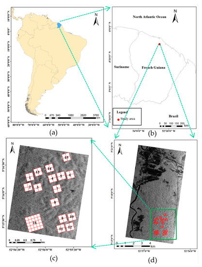
Figure 1.
Overview of study area. The map (a) shows location of French Guiana in South America. The red dot in (b) map is the geographical location of the study area. In the (d) image, the base map on the right is synthetic aperture radar (SAR) (HV polarization) data and the green box over the SAR data is the study area, and the red boxes inside the study area are the sample plot locations. The (c) image shows the division strategy of 16 fixed plots.
In this study, six flight passes of airborne P-band Quad-pol (HH, HV, VH, VV) SAR dataset were acquired during the TropiSAR aviation campaign. The TropiSAR campaign was conducted in French Guiana in the summer of 2009 in the framework of the Phase A studies pertaining to the BIOMASS mission, one of the three for Earth Explorer candidates [39]. SAR data was acquired by the airborne system SETHI at the Paracou in August and total rainfall in August was 49 mm (8 days with rainfall) [39]. Despite the fact that this SAR dataset has been used in forest parameter estimation of TomoSAR, in our study, more features were mined for forest AGB estimation through dataset. The parameters of SAR dataset are shown in Table 1. The SAR dataset has been preprocessed by registering, radiometric correction, removing flat earth effect and phase calibration.

Table 1.
Parameters of SAR dataset.
LiDAR data (DTM and DSM) covering the study area was provided by the CIRAD. It was used to verify the forest vertical profile extracted by TomoSAR. The LiDAR coverage data was acquired using the ALTOA system in 2009, operating a helicopter-borne LiDAR with about 150 m above the ground flying height [39,42]. The laser wavelength was 0.9 μm, scanning angle was ±30°, and the recorded last reflected pulse was better than 0.1 m. The mean number of pulses per m2 on a single acquisition was 4 [42], and DTM and DSM products (Figure 2) with spatial resolution of 1 × 1 m was produced by the original LiDAR point cloud data. The DTM and the DSM was filtered using a conditional median filter (applied once) whereby any cell having 7 or 8 neighbors (out of 8) 2 m lower than target cell was replaced by median value of neighborhood [41]. The coordinate systems of DTM and DSM products were WGS84 and the projections were Universal Transverse Mercator (UTM) [39].
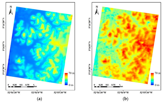
Figure 2.
LiDAR data of study area. (a) DTM products of LiDAR, (b) DSM products of LiDAR.
The forest AGB field survey data collected based on forestry censuses also comes from CIRAD. The forestry censuses were conducted in 2009 and 2010 [39]. During the field survey, the 16 fixed plots were set up in the study area, including 15 plots (No. 1–15) with the size of 250 m × 250 m and 1 plot (No. 16) with the size of 500 m × 500 m (Figure 1c). In order to increase the number of sample plots for statistical analysis like the relationships between forest AGB and features for estimation, the field survey data of AGB sample plots used in this paper were sub sampled into 85 in total, which were divided from the fixed plots. The division strategy (Figure 1c) was as follows: Each fixed plot (No. 1–15) was divided into 4 sub sample plots (125 m × 125 m), with a total of 60 sub sample plots and No. 16 fixed plot was divided into 25 sub sample plots (100 m × 100 m). The field survey data includes the DBH of each tree in a fixed plot (DBH > 10 cm), which was used to calculate the biomass of each tree with allometric growth functions according to different tree species. The methods and more details for AGB calculation were given in the references [39,43]. The AGB (Mg∙ha−1) of each sub sample plot was the sum of that of each tree in the sub sample plot. The mean forest AGB of the 85 sub sample plots ranges from 250 to 450 Mg∙ha−1, and the details information of the forest AGB ground truth data are shown in Table 2. The sample plots with AGB level of 0~300 Mg∙ha−1, 300~400 Mg∙ha−1, and 400~500 Mg∙ha−1 are shown in Figure 3.
Table 2.
Forest aboveground biomass (AGB) data of sub sample plots.

Figure 3.
Sample plots with different biomass level. (a) Biomass level: 0~300 Mg∙ha−1; (b) biomass level: 300~400 Mg∙ha−1; (c) biomass level: 400~500 Mg∙ha−1.
2.2. Framework of Research
At present, there are many literatures that introduce the basic theory of TomoSAR. For the detailed introduction of TomoSAR theory, please refer to literature [7,28]. The framework of this study is shown in Figure 4. The main contents of the study include: (1) Constructing covariance matrix of full-polarization TomoSAR data set, the SKP decomposition and algebraic synthesis algorithm were used to extract the ground and volume scattering covariance matrices respectively. After PolTomoSAR imaging, we got the vertical profile of PolTomoSAR. According to the distribution of backscattered power from ground scattering and volume scattering respectively, the DTM and DSM were produced [7,38,41,44]. (2) The DTM obtained in (1) was used to remove the ground phase of HV polarimetric SAR data, and the backscattered power was obtained after tomographic SAR imaging, then the backscattered power was processed by terrain compensation. (3) The best spectrum analysis algorithm was selected as the tomographic imaging method for further analysis according to the matching degree between the backscattered power distribution of vertical profile and LiDAR CHM products (DSM minus DTM). (4) The extracted multi-height layers backscattered power was geocoded and fitted to obtain the backscattered power curve of vertical profile. (5) Vertical profile features such as the BPFAH and the LBPC etc. were extracted from the fitted backscattered power curve, and those features were used in regression modeling, then the forest AGB was estimated and the accuracy was evaluated by field survey data.
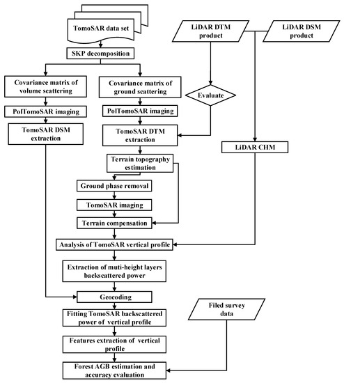
Figure 4.
The framework of this study.
2.3. TomoSAR Data Processing and Tomographic Imaging Algorithm
The production of TomoSAR vertical profile is the fundamental part of forest AGB estimation. The key steps mainly include tomographic SAR data preprocessing, ground phase removal, tomographic imaging and terrain compensation. After careful SAR data preprocessing operations, such as radiometric calibration, polarimetric SAR calibration, accurate registration and flat earth effect removal, the SAR data set used in this study meets the requirements of tomographic imaging [39]. The TomSAR data set consisted of 6 flight passes, allowing the formation of interferograms with vertical wavenumbers between 0.02 and 0.3 rad/m and a Rayleigh height resolution limit of TomoSAR data set is about 10 m. After the tomographic imaging, it can achieve the estimation ability of 1 m that can accurately describe the forest component within forest height range of 20 to 40 m [45,46]. For more detail information about SAR data preprocessing, readers are referred to the TropiSAR campaign related literature [39]. In the follows, we mainly described the procedures of ground phase removal, tomographic imaging and terrain compensation.
2.3.1. Ground Phase Removal
Knowledge of terrain topography is required for removing ground phase and compensating the backscattered power measurements for the local terrain slope, as well as for mapping the multilayer data stack onto ground geometry [28]. In this paper, terrain topography has been estimated by PolTomoSAR imaging, which was described in [38].
In forest area, the phase information in the SAR data contains two parts: One part comes from the ground under forest canopy, another part comes from the forest vegetation above the ground, as shown in (1) if we neglect other phase errors sources.
where is the total phase information of SAR data, is that of the forest, Hg is the elevation of ground under the forest canopy, which can be derived from the DTM product of PolTomoSAR imaging and the represents the phase information corresponding to the ground. After removing from , the retained phase information mainly corresponds to the phase that forest vertical structure caused. In this way, the TomoSAR backscattered power profile dominated by forest can be obtained.
2.3.2. Tomographic Imaging
After ground phase removal, the tomographic imaging was carried out to obtain the TomoSAR forest vertical profile. The key algorithm of tomographic imaging is spectrum analysis. Since Beamforming, Capon, and MUSIC algorithms have certain representativeness, need relatively small amounts of calculation, and are more mature stage of development, in this paper, we compared the effectiveness of the three spectrum analysis algorithms [38]. Concerning the size of sub sample plots and resolution of SAR data, the spectrum analysis algorithms had been applied by processing 40 independent looks, corresponding to a squared multilook cell with 50 m side length. The forest height product (CHM) was obtained by the difference between DTM and DSM products of LiDAR. Then the matching degree between the backscattered power distribution of TomoSAR vertical profile and CHM by LiDAR was used to validate the effectiveness of each spectrum analysis algorithm. Finally, we chose the algorithm that matches LiDAR CHM best for further data analysis.
2.3.3. Terrain Compensation
For backscattered power of TomoSAR, except for the forest on the surface, the topographic relief in the SAR illuminating area can also lead to the changes of backscattered power. The topographic relief will affect the imaging geometry of TomoSAR, and then affect the extracted TomoSAR backscattered power. In order to eliminate the influence of topographic relief on the backscattered power, we need compensate the terrain effects on TomoSAR data set.
Firstly, the slope angle at the illuminating area in one SLC pixel was calculated by the DTM obtained from the SAR data set itself using SKP decomposition and PolTomoSAR imaging. Secondly the local incidence angle of each pixel in SLC image was calculated by the incidence angle and slope angle of the SAR imaging systems. Finally, the intensity of each pixel of the image can be compensated using Equation (2).
where, is of complex-value corresponding to pixel at SAR imaging coordinate within the multi-height layers data stack produced by the tomography processing, with r is the slant range and x is the azimuth. is the incidence angle of SAR system, is the local slope angle, is terrain compensation factor and is the backscattered power after terrain compensation.
2.4. Feature Extraction of Forest Vertical Profile Based on TomoSAR
2.4.1. Main Factors Affecting Forest AGB at a Sample Plot Scale
From the perspective of dendrometry theory, the main factors closely related to forest AGB at a plot scale mainly include: Forest average height [36,47], stand density [37,48], average DBH [48], and multi-storied forest [49]. In the actual situation, assuming that only a single factor influence on the forest AGB is considered, the relationship between the single factor and the forest AGB can be illustrated by Figure 5. For example, the upward arrow of the Figure 5 shows that the forest AGB increases with the average height, if the forest stand has the same density, average DBH and single-storied forest. While the downward arrow of Figure 5 shows that if two forest stands are the same average height, density and average DBH, the one with multi-storied forest will have higher forest AGB.
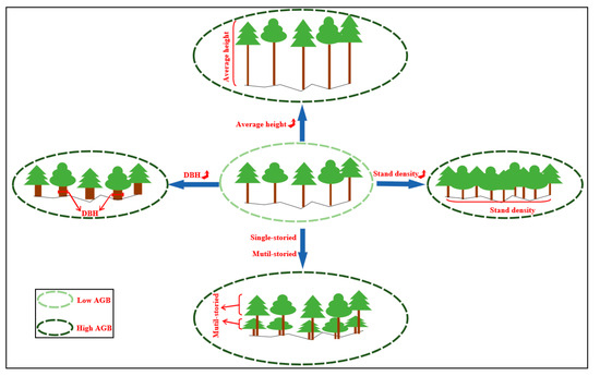
Figure 5.
Simplified relationship between factors of dendrometry and forest AGB.
TomoSAR technique has the 3D capability of observing forest vertical structures [50]. As shown in Figure 6, TomoSAR can not only produce the vertical profile, but also extract the backscattered power of the multi height layers in the irradiation area. The backscattered power of the multi height layers belongs to the information of horizontal dimension (Figure 6), so the backscattered power at specific height layer can reflect the horizontal information of forest at corresponding height. For example, without considering the influence of ground scattering, the backscattered power at 5 m height layer contains some horizontal information such as DBH and stand density. Otherwise, through the backscattered power distribution in the vertical profile, we could obtain forest average height, multi-storied and other structure information in the vertical dimension. Since all of them are partially related with forest AGB, we can define some features to fully characterize the vertical power profile that related with the factors of dendrometry, by this way to improve forest AGB estimation accuracy.
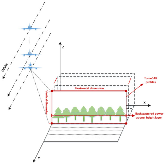
Figure 6.
Schematic diagram of forest 3D observation by Tomographic SAR (TomoSAR).
2.4.2. Fitting of Backscattered Power Curve and Features Extraction
After tomographic imaging, we geocoded the backscattered power of vertical profile from TomoSAR and then the backscattered power was transformed from radar imaging geometry to ground geometry. In order to quantitatively describe the backscattered power of the vertical profile, we fitted the backscattered power at a sample plot scale, and obtained the backscattered power curve of the forest vertical profile. Li et al. defined 10 parameterized features according to the extracted vertical profile by PCT [4], and these features can describe the geometric characteristics of vertical profile, but they cannot highlight the concentration distribution characteristics of backscattered power on elevation direction of vertical profile. In order to better describe the forest vertical profile, we used the spatial rectangular coordinate system (x, y, z) to denote the horizontal and vertical dimension in the ground geometry. Based on the analysis of factors affecting forest AGB at a sample plot scale in Section 2.4.1, we proposed some features that are more closely related to the factors of dendrometry. The extracted features in this way were presented as the follows:
- In the horizontal dimension of the ground geometry, which we called (x, y) plane, the parameterized samples of TomoSAR vertical profile were selected according to sub sample plot position recorded by the field survey. In this paper, 85 sub sample plots were used, including 25 sub sample plots of size 100 × 100 m and 60 sub sample plots of size 125 × 125 m. The sizes of sub sample plots were about the same as four multilook cells, and each sub sample plot (100 × 100 m or 125 × 125 m) corresponded to a backscattered power curve.
- In the vertical dimension of ground geometry, on the z axis of spatial rectangular coordinate system, the height range of 0–40 m was sampled at an interval of 1 m, with a total of 40 sampling height layers.
- At the sampling height layers determined in (2), the backscattered power of the TomoSAR vertical profile was sampled, so the backscattered power mean values in the height range of 0–40 m (1 m interval) were obtained for each of the 85 sub sample plots.
- Because some features’ calculation needs to convert the discrete backscattered power value into continuous power curve, such as the LBPC and BPFAH, the backscattered power mean value of each sample in the vertical direction was fitted using the Gaussian Mixture Model [4,18]. The fitting performance was evaluated by fit goodness, and R-square of backscattered power curve fitting in all sub sample plots were above 0.98. Finally, we obtained the backscattered power curves of 85 sample points ranging from 0 to 40 m.
- Based on the difference between DTM and DSM products [7,38], we averaged the forest height of the 85 samples. The backscattered power curve of vertical dimension was limited according to the average forest height. Then the backscattered power curve of TomoSAR vertical profile within the range of forest height was obtained.
- Based on the backscattered power curve fitted in (5), the features of TomoSAR vertical profiles were extracted. The features included the LBPC, the BPV of the TomoSAR at intervals of 1 m within the range of forest height, the BPFAH and the FAH. The definitions of these proposed features were listed in Table 3.
Table 3. Definition of the features extracted from TomoSAR forest vertical profile.
All the features in Table 3 made use of the backscattered power distribution, which depended not only on forest structure, but also on the physical parameters such as dielectric properties of the forest. Weather conditions, such as rainfall, can change the dielectric properties of forest structure, thus affecting the backscattered power distribution in TomoSAR vertical profiles. SAR backscattering from forest is mainly related to the dielectric constant of forest tissue, which depends strongly on the water content of forest tissue. In the process of rainfall, the canopy can retain up to a certain amount of water, above which the extra amount drops to the ground, increasing moisture [34,51]. It was apparent that after the rainfall the backscattered power of ground was in general reduced with respect to the backscattered power of canopy [34,51]. However, the change of dielectric properties had a relative impact on the TomoSAR forest AGB estimation result and the estimation accuracy mainly depended on the forest structure [23]. Moreover, the acquisition data of the 6-track TomoSAR data set used in this paper was less than one day, and their time baseline was about 2 h [39]. The time of data acquisition was short, and there was no rain in a few days during data acquisition, so the dielectric properties of the forest were relatively stable. Those features extracted from TomoSAR vertical profile can still reflect the information of forest structural, which was used for forest AGB modeling and estimation.
2.5. Forest AGB Estimation and Accuracy Validation
After completing the feature extraction of TomoSAR vertical profile, we carried out the correlation analysis (Pearson correlation) between the extracted feature set and the ground measured forest AGB. Then, 65% of the 85 plots (55 plots) were randomly selected for linear regression modeling. The linear regression model is shown in (3). Finally, the remaining 35% of the plots (30 plots) were used for the accuracy validation. We adopt the absolute accuracy in percentage and the root mean square error (RMSE) as shown in (4) and (5) as accuracy validation indexes.
where, is the estimated forest AGB, ,… is features of TomoSAR vertical profile, is constant of regression model and is the forest AGB measured by the plot i (i = 1, 2, …, n), p is the number of variables, and n is the plot number (30), and is the mean AGB of the n forest plots.
3. Results
3.1. TomoSAR Data Processing
At forest covered area, different polarimetric SAR data has different scattering mechanisms, and their performance in forest biomass estimation is also different. Relevant contributions from the ground level beneath the forest are observed. In HH and VV, the ground contribution is more important than the contribution of the forest, while in HV the contribution of the ground layer appears less important than that of the forest layers [28]. In this paper, we pay more attention to the contribution from forest in scattering mechanism, so we choose HV polarization to estimate forest AGB.
3.1.1. The Effectiveness of Terrain Topography Estimation and Terrain Compensation
The DTM product of terrain topography estimation was shown in Figure 7a, which was used to do ground phase removal and terrain compensation. A comparison with the available analysis of LiDAR DTM had shown the absolute accuracy greater than 87% and RMSE was less than 2.5 m. The scatter density plot of LiDAR DTM and PolTomoSAR DTM was shown in Figure 8.
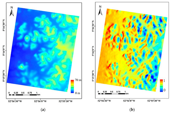
Figure 7.
DTM product of polarimetric interferometric SAR (Pol-InSAR) (a) and terrain compensation factor (b) of the study area.
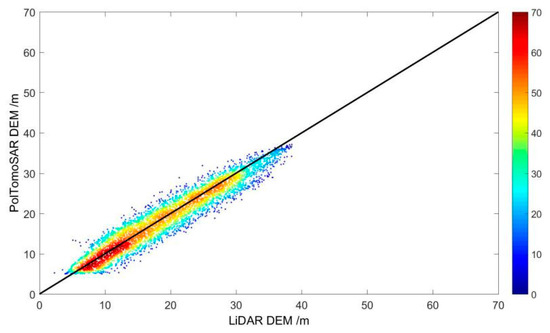
Figure 8.
Scatter density plot of LiDAR DTM and PolTomoSAR DTM.
Terrain compensation is a key step in the accurate estimation of forest AGB with TomoSAR. The DTM product and terrain compensation factor obtained for terrain compensation processing were shown in Figure 7.
The results of terrain compensation were firstly evaluated and analyzed by comparing the TomoSAR vertical structure profile and horizontal dimension backscattered power distribution before and after terrain compensation. Figure 9 showed the backscattered power distribution of TomoSAR forest vertical profile before and after terrain compensation. The black line in the Figure 9 represented the plane with an altitude of 0 m and the white line represents the forest height extracted by using the CHM products of LiDAR. Figure 9a showed the results before terrain compensation, Figure 9b was the results after terrain compensation. Through the comparative analysis of them, we found that the terrain had a certain influence on the backscattered power distribution of the TomoSAR vertical profile. We found that the backscattered power distribution of the forest canopy in the vertical profile became discontinuous, which may be due to the influence of terrain factors. After terrain compensation, the backscattered power in the forest canopy of the vertical profile is compensated obviously and the backscattered power in the canopy shows more continuous in the compensated image.
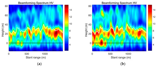
Figure 9.
TomoSAR forest vertical structure profile. (a) Before terrain compensation; (b) after terrain compensation.
Secondly, the qualitative evaluation was made by analyzing the changes of backscattered power distribution before and after terrain compensation in horizontal dimension. The results show obvious difference of backscattered power distribution before and after terrain compensation. In the area seriously affected by topographic relief, terrain compensation had corrected the difference of backscattered power between radar illumination area and shadow area. In the forest scattering mechanism, the scattering from the ground and trunk is the main scattering mechanism in the forest near the ground height, and the volume scattering is the main scattering mechanism near the canopy height. With the increase of height, the scattering contribution of the ground becomes smaller and smaller, while that scattering contribution of the trunk and canopy increases gradually [28]. In the middle part of the forest height, the main scattering contribution is coming from mixed scattering of trunk and canopy. According to the statistics, the average forest height is about 30 m in study area. In order to reflect the efficiency of terrain compensation on trunk and canopy scattering more comprehensively, the backscattered power of 15 m height layer was chosen as an example to show in Figure 10, which was in the middle of the forest average height. In addition to the correction of the overall distribution of power on SAR image, the difference in the backscattered power distribution caused by the different slope directions in the regions with large topographic relief had been corrected.
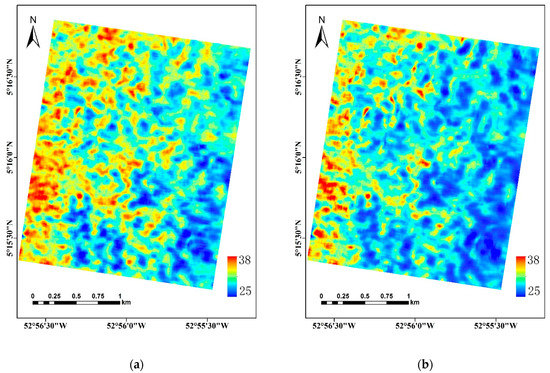
Figure 10.
Backscattered power of 15m height layer. (a) Before terrain compensation; (b) after terrain compensation in the right image.
Lastly, the effectiveness of the terrain compensation was also quantitatively evaluated by comparing the correlation between the backscattered power and the forest AGB. It was found that the correlations of each height layer with forest AGB were enhanced after terrain compensation. For example, as shown in Figure 11, the Pearson correlation coefficient (r) between the backscattered power of the 15 m height layer and the forest AGB was increased from 0.22 before terrain compensation to 0.27 after compensation.
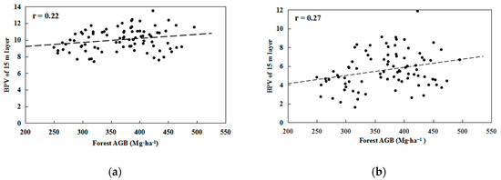
Figure 11.
Correlation of backscattered power and forest AGB before (a) and after (b) terrain compensation in 15 m height layer.
The above analysis showed that after terrain compensation, the backscattered power of TomoSAR had been significantly corrected, and the correlation between backscattered power and forest AGB had been improved. The topographic relief effects on the distribution of backscattered power of TomoSAR were obviously reduced.
3.1.2. Tomographic SAR Imaging
In order to analyze the results of spectrum analysis algorithm more objectively, we evaluated the fitting degree of forest height products extracted from LiDAR and TomoSAR vertical profile by three kinds of spectrum analysis algorithms. As shown in Figure 12, the TomoSAR vertical profiles with line numbers of 100, 200, and 500 in SLC image were selected and displayed here. The white lines in the vertical profiles were the forest height curve extracted by LiDAR (CHM), and the black lines were the elevation of 0m. Normally, the profile power can be concentrated in the scattering center of the forest canopy and the ground. Compared with the other two spectrum analysis algorithms, the backscattered power distribution in the vertical profiles extracted by Beamfroming algorithm was highly consistent with the forest height curve extracted from LiDAR. We also analyzed the backscattered power distribution in the forest canopy height range from the horizontal dimension. The backscattered power distribution continuity calculated from Capon algorithm was shown to be worst among three algorithms, and the results of MUSIC and Beamfroming were better. In the vertical dimension of backscattered power distribution, the backscattered power of MUSIC algorithm was mostly concentrated in the two scattering centers of the canopy and the ground, and the backscattered power from forest part scattering above the ground was very small. In contrast, the results of Beamforming algorithm can better describe the distribution of backscattered power from forest scattering in the vertical dimension. Therefore, the Beamforming algorithm were chosen in this study to image the vertical profile and extract the features for forest AGB estimation.
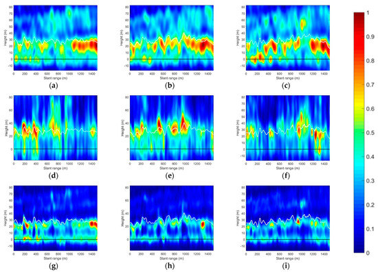
Figure 12.
TomoSAR vertical profile of Beamfroming, Capon, and MUSIC. The white curve in vertical profile is LiDAR forest height product (CHM) and the black line in vertical profile is altitude of 0 m. (The top panels are imaging results of Beamforming, the middle panels imaging results of Capon, and the low panels are imaging results of MUSIC; the (a,d,g) are imaging results of 100 row in SLC image, the (b,e,h) are imaging results of 200 row in SLC image, the (c,f,i) are imaging results of 500 row in SLC image).
3.2. Analysis of the Relationship between Profile Features and Forest AGB
3.2.1. Backscattered Power Curve Fitting Results and Their Characteristics in Different AGB Levels
After tomographic SAR imaging, we fitted the backscattered power curves of the 85 sub sample plots and analyzed the characteristics of typical backscattered power curves averaged for the plots in three AGB levels. Figure 13 showed the mean backscattered power curves of sub sample plots with AGB 0~300 Mg∙ha−1, 300~400 Mg∙ha−1, and 400~500 Mg∙ha−1. The general relationship between the shape of the curve and the AGB level were summarized as follows:
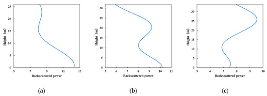
Figure 13.
Typical backscattered power curve of sub sample plots with different biomass level. (a) Biomass level: 0~300 Mg∙ha−1; (b) biomass level: 300~400 Mg∙ha−1; (c) biomass level: 400~500 Mg∙ha−1.
(1) When the forest AGB was at a lower level (AGB < 300 Mg∙ha−1), the peak position of the backscattered power curve of most of the sub sample plots was close to the ground, mainly varied in the lower altitude range.
(2) With the increase of forest AGB level (300 Mg∙ha−1 < AGB < 400 Mg∙ha−1), the peak position of backscattered power curve of most of the sub sample plots gradually moved up, while the second peak appeared.
(3) When the forest AGB reached a high level (AGB > 500 Mg∙ha−1), the peak position gradually approached to the top of forest canopy, and varied in the upper altitude range.
3.2.2. Analyzing the Sensitivity of the Profile Features to Forest AGB
Figure 14 showed the correlations between the vertical profile features and the forest AGB of the 85 sub plots. Here, BPV-31 is the BPV at 31 m height layer, and BPV-5 was the BPV at 5 m height layer. It showed that the BPV-5 and BPV-31 had increased r values with forest AGB, amounts to −0.647, 0.654 respectively. While the r values for the relationship between forest AGB and FAH (denoted as r for FAH) was 0.684, that for LBPC was 0.602, for BPFAH was 0.706. All of the 5 features showed significantly sensitive to the forest AGB, among them, BPFAH is the most sensitive one.
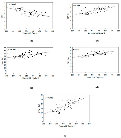
Figure 14.
Correlation between the profile features and forest AGB. (a) BPV of 31m height layer, (b) BPV of 5m height layer, (c) LBPC, (d) FAH, (e) BPFAH.
In [28,30], the Capon spectrum analysis algorithm and 5-m interval sampling methods were applied to extract the backscattered power in the z-axis direction. The r value between the BPV-30 and the forest AGB was the highest and they concluded that BPV-30 was the best feature for forest AGB estimation. Studies in [45,46] had shown that because the high semitransparency of the canopy, and the possibility has been demonstrated to reach an estimation precision in the order of magnitude of 1 m, even with non-model-based TomoSAR approaches. However, in order to get more accurate backscattered power curves to describe the power distribution in TomoSAR vertical profile at a sample plot scale, the sampling interval of 1 m was applied in this paper, and the Beamforming spectrum analysis algorithm which has better performance in LiDAR forest height products matching was selected for TomoSAR imaging. Further, we selected BPV-5, BPV-31, LBPC, FAH, and BPFAH, which can reflect forest vertical structure information and sensitive to forest AGB, as features to estimate forest AGB.
3.2.3. Accuracy Validation
At present, BPV-30 was the commonly used feature to estimate forest AGB by TomoSAR [28,30]. In addition, there are studies on forest AGB estimation by using backscattered power at multiple height layers (BPV-5 and BPV-30) as estimating features [7,38]. In order to verify the validity of the method proposed in this paper, we validated the accuracy of the model taking the BPV-30 as unique feature (predictor) and the BPV-5 and BPV-30 as multi features (predictors) in estimating forest AGB. The 30 sub plots data were randomly selected for model validation. The result of taking BPV-30 as unique feature was shown in Figure 15, the absolute accuracy was 86.70%, and the RMSE was 58.65 Mg∙ha−1. Figure 16 showed the result of taking BPV-5 and BPV-30 as multi features, the absolute accuracy was 89.52%, and RMSE was 43.08 Mg∙ha−1. While the accuracy of the proposed multi-features-based modeling method with all the five features as predictors was shown in Figure 17, its accuracy was 90.73%, and RMSE was 42.45 Mg∙ha−1. Compared with taking BPV-30 as unique feature, taking both BPV-5 and BPV-30 as features, the proposed multi features (5 features involved) based modeling method increased the accuracy by 4.03%, 1.21% respectively, and decreases the RMSE by 16.2 Mg∙ha−1, 0.63 Mg∙ha−1 respectively. The result showed that the method proposed in this paper had better performance than the published methods.
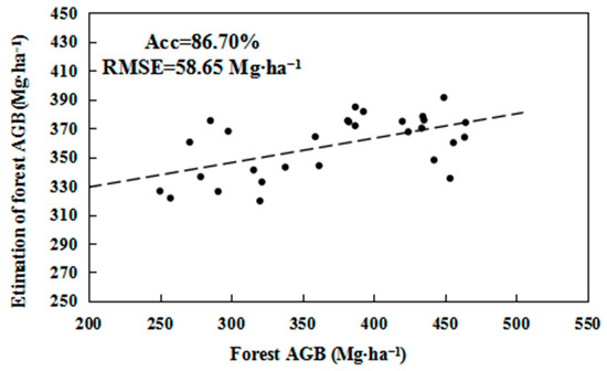
Figure 15.
Scatter plot of ground observed with estimated forest AGB by the model taking the BPV-30 as unique feature.
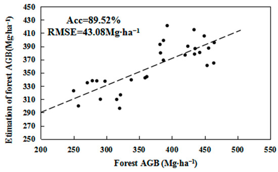
Figure 16.
Scatter plot of ground observed with estimated forest AGB by the model taking the BPV-5 and BPV-30 as features.
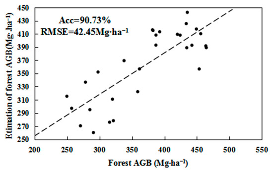
Figure 17.
Scatter plot of ground observed with estimated forest AGB by the proposed multi-features-based model method.
4. Discussion
This paper proposed a multi-features-based modeling method for forest AGB estimation. The proposed method using BPV-31, BPV-5, LBPC, FAH, and BPFAH as features to estimate forest AGB. In order to better understand the effectiveness of the features proposed in this paper, the r values between each of the five features (Table 3) were calculated and listed in Table 4 respectively. It showed that BPFAH had strong correlations with other features, and the r values were above 0.7. Although LBPC had strong correlations with BPFAH and FAH, and both r values were more than 0.7, the correlations between LBPC and the other features were relatively weak. The correlations between FAH and other features were high, and the r values between FAH and BPV-5, BPFAH, and LBPC were all over 0.8. Among them, the correlations between BPV-31 and other features were the weakest. Among 5 features, BPV-5 and BPV-31 reflected the horizontal information of the backscattered power from trunk and canopy respectively, while FAH reflected the forest height information and LBPC mainly reflected the multi-storied forest information in vertical dimension. In terms of correlation, except for BPV-5 and FAH, a weak correlation between the features that reflecting forest horizontal information and vertical information. BPFAH was the comprehensive expression of the forest height information (vertical dimension) and the backscattered power of forest parts at multiple height layers (horizontal dimension). Compared with other features, BPFAH had more comprehensive information about forest structure, and then it had the highest correlation with forest AGB. Although the correlation between LBPC and forest AGB is weaker than that of BPFAH, and LBPC was more independent and can better supplement other features for forest AGB estimation.
Table 4.
Correlation between the 5 features.
In the methods of forest AGB estimation using TomoSAR, the BPV-30 and BPV-5 are two commonly used features for estimation [7,28,29,30,33,38]. Generally, after the same data processing and regression modeling, the result of estimation showed that BPV-30 as the single feature to estimate forest AGB had the quite good accuracy and RMSE [28,29,30,33]. Further, the method used both BPV-5 and BPV-30 as features obtained higher accuracy and lower RMSE. It meant that BPV-5 can improve the accuracy of estimation, which is consistent with [7,38]. Being compared with BPV-30, BPV-5 was more susceptible to the perturbing effect of the ground contribution [28]. However, BPV -5 may well reflect the situation of forest trunk, which was closely related to DBH and stand density, the two main factors strongly related with forest AGB. Therefore, this paper also uses BPV-5 as a feature to estimate forest AGB. Compared with [28,29,30,38], we found that BPV-31 has higher correlation with AGB than BPV-30, and used it as a feature to estimate AGB. It may result from the smaller sampling interval (1 m) to extract the backscattered power in the vertical direction.
In the tropical area, many forests belong to multi-storied forest which may has wider height range of canopy than single-storied forest. Under the same forest growth, the wider height range of canopy means higher canopy backscattering power. The LBPC describes forest backscattering in vertical profile, and forest backscattering is mainly determined by canopy backscattering and forest height. Therefore, LBPC reflects the information of forest height and multi-storied forest. The BPFAH is calculated by backscattered power in horizontal dimension and forest height in vertical dimension, so the information reflected by BPFAH is more comprehensive. The last feature, FAH, is directly related to forest average height. Therefore, the features in Table 4 can not only reflect the more information of forest vertical structure, but also have a closer relationship with the factors of dendrometry. In addition to the features in Table 4, it seems that different forest AGB levels for the same height can be expressed as through a variation of the ground-to-volume power ratio (Figure 13). The ground-to-volume power ratio can well reflect the relationship between the AGB level and the concentration of backscattered power. However, the ground-to-volume power ratio only reflects the distribution of backscattered power at different biomass levels, and is not a more direct description of measurement factors, such as forest height, DBH and other factors, which is different from the focus of this study, so we did not use ground-to-volume power ratio as the forest AGB estimation feature in this paper.
To interpret the performance and potentiality of the proposed method in this paper, we compared the spatial distribution of the estimated forest AGB with CHM product of LiDAR (Figure 18). The result of forest AGB estimation (Figure 18b) showed that the biomass level of the study area ranged from 200 to 500 Mg∙ha−1. From Figure 18a,b, we can see a high consistency between the estimated biomass and forest height in CHM acquired by LiDAR. We took fixed plots of No.1 (sub plot No. 1–4), No. 8 (sub plot No. 29–32) and No. 16 (sub plot No. 61–85) as examples, the forest AGB data (Table 2) shows that the biomass levels of fixed plot No. 1, No. 8 and No. 16 are about 370 Mg∙ha−1, 260 Mg∙ha−1 and 406 Mg∙ha−1 respectively. By observing the location of the corresponding fixed plots in Figure 18b, we found that the estimated AGB values from TomoSAR dataset were consistent with the AGB in Table 2. However, in some areas where the forest height changes dramatically, such as the left side of the result map, the estimated AGB are relatively insensitive to CHM. This may be related to some errors in TomoSAR data acquisition or imaging geometry, which will lead to the difference of backscattered power distribution in TomoSAR profiles, which then affect the estimation accuracy of method in this study.
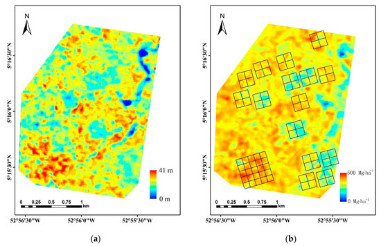
Figure 18.
LiDAR-derived Canopy Height Model (CHM) (a) and the forest above-ground biomass (AGB) estimation from TomoSAR dataset (b).
Although proposed method in this paper has good accuracy, there are still some issues need for further research. It is believed that with the continuous development of TomoSAR technique, the accuracy of this study will be further improved under the conditions of more flight passes and higher resolution of TomoSAR data. In this paper, the role of polarimetric information in the forest AGB estimation has not been studied deeply. The polarimetric information is useful for separating the scattering mechanism of the ground and removing perturbing effect of the ground contribution. After removing the ground contribution, we can get a simpler forest scattering mechanism information. Based on that, the accuracy of forest AGB estimation may be further improved. Therefore, how much polarimetric information can contribute to the forest AGB estimation should be further explored in the future.
5. Conclusions
AGB is a key parameter of forest, and it is widely used in forest resources management. This paper mainly focuses on the extraction of multi features from TomoSAR vertical profile which are closely related to the key factors relevant to forest AGB according to the dendrometry theory. Based on this, some feature such as BPV-31, BPV-5, LBPC, FAH, and BPFAH were proposed to estimate forest AGB.
The result shows that, in addition to the good correlation between the BPV of TomoSAR at specific height layer and the forest AGB, other features proposed in this paper also have a good correlation with the forest AGB, and all of the r values between these features and forest AGB are above 0.6. Among all the features of TomoSAR vertical profile, the BPFAH has the best correlation with forest AGB, and the r value between them is more than 0.7. The results of correlation analysis also show that the features of vertical profile extracted in this paper can be used to estimate forest AGB. In order to evaluate the forest AGB estimation capability of the proposed method, 55 sample plots data were used for linear regression modeling and 30 sample plots data were left for accuracy verification. The absolute accuracy is 90.73% and RMSE is 42.45 Mg∙ha−1 by our proposed method. The forest AGB estimation performance using the proposed method is significantly improved compared with published methods applied to the same study site and dataset.
To conclude, in this paper the new features of TomoSAR profile has been exploited for the retrieval of AGB in tropical forests. The methodology based on TomoSAR multi-features to derive the AGB has been described. Overall, we have proved that the new features defined in this paper can further improve the forest AGB estimation accuracy. The methodology and the results can apply to the dense tropical forest, even over areas with topography. Finally, despite the much work that remains to be done, the method proposed in this paper need further explored in other forest types.
Author Contributions
Conceptualization, X.W., Z.L., E.C., and L.Z.; Formal analysis and writing—original draft preparation X.W., Z.L., E.C., L.Z., W.Z., and K.X. All authors contributed to interpreting results and the improvement of the paper. All authors have read and agreed to the published version of the manuscript.
Funding
This research was funded by National Key R&D Program of China, grant number 2017YFB0502700 and National Natural Science Foundation of China, grant number 41801289 and grant number 31860240.
Acknowledgments
We thank the National Key R&D Program of China (Grant No. 2017YFB0502700) and National Natural Science Foundation of China (Grant No.41801289). for financial support, and the European Space Agency (ESA) for data support. Acquisition cost of the LiDAR data was covered by European Regional Development Fund, convention # 2907 dated 4 November 2008.
Conflicts of Interest
The authors declare that they have no conflict of interest.
References
- Galbraith, D.; Levy, P.E.; Sitch, S.; Huntingford, C.; Cox, P.; Williams, M.; Meir, P. Multiple mechanisms of Amazonian forest biomass losses in three dynamic global vegetation models under climate change. New Phytol. 2010, 187, 647–665. [Google Scholar] [CrossRef] [PubMed]
- Köhl, M.; Lasco, R.D.; Cifuentes, M.; Jonsson, Ö.; Korhonen, K.; Mundhenk, P.; Návar, J.; Stinson, G. Changes in forest production, biomass and carbon: Results from the 2015 UN FAO Global Forest Resource Assessment. For. Ecol. Manag. 2015, 352, 21–34. [Google Scholar] [CrossRef]
- Reich, P.B.; Luo, Y.; Bradford, J.B.; Poorter, H.; Perry, C.H.; Oleksyn, J. Temperature drives global patterns in forest biomass distribution in leaves, stems, and roots. Proc. Natl. Acad. Sci. USA 2014, 111, 13721–13726. [Google Scholar] [CrossRef] [PubMed]
- Li, W.; Chen, E.; Li, Z.; Ke, Y.; Zhan, W. Forest aboveground biomass estimation using polarization coherence tomography and PolSAR segmentation. Int. J. Remote Sens. 2015, 36, 530–550. [Google Scholar] [CrossRef]
- Rodríguez-Veiga, P.; Quegan, S.; Carreiras, J.M.; Persson, H.J.; Fransson, J.E.; Hoscilo, A.; Ziółkowski, D.; Stereńczak, K.; Lohberger, S.; Stängel, M.; et al. Forest biomass retrieval approaches from earth observation in different biomes. Int. J. Appl. Earth Obs. Geoinf. 2019, 77, 53–68. [Google Scholar] [CrossRef]
- Gu, C.; Clevers, J.G.; Liu, X.; Tian, X.; Li, Z.; Li, Z. Predicting forest height using the GOST, Landsat 7 ETM+, and airborne LiDAR for sloping terrains in the Greater Khingan Mountains of China. ISPRS J. Photogramm. Remote Sens. 2018, 137, 97–111. [Google Scholar] [CrossRef]
- Li, L.; Chen, E.; Li, Z.; Zhao, L.; Gu, X. Forest above ground biomass estimation from P-band tomography data. In Proceedings of the 2016 IEEE International Geoscience and Remote Sensing Symposium (IGARSS), Beijing, China, 10–15 July 2016; IEEE: Piscataway, NJ, USA, 2016; pp. 21–23. [Google Scholar] [CrossRef]
- Luo, H.; Chen, E.; Cheng, J.; Li, X. Tree height retrieval methods using POLInSAR coherence optimization. In Proceedings of the 2010 IEEE International Geoscience and Remote Sensing Symposium, Honolulu, HI, USA, 25–30 July 2010; IEEE: Piscataway, NJ, USA, 2010; pp. 3259–3262. [Google Scholar]
- Cutler, M.E.J.; Boyd, D.S.; Foody, G.M.; Vetrivel, A. Estimating tropical forest biomass with a combination of SAR image texture and Landsat TM data: An assessment of predictions between regions. ISPRS J. Photogramm. Remote Sens. 2012, 70, 66–77. [Google Scholar] [CrossRef]
- Luckman, A. A study of the relationship between radar backscatter and regenerating tropical forest biomass for spaceborne SAR instruments. Remote Sens. Environ. 1997, 60, 1–13. [Google Scholar] [CrossRef]
- Mette, T.; Papathanassiou, K.P.; Hajnsek, I.; Zimmermann, R. Forest biomass estimation using polarimetric SAR interfer-ometry. In Proceedings of the International Geoscience and Remote Sensing Symposium, Toronto, ON, Canada, 24–28 June 2002; IEEE: Piscataway, NJ, USA, 2002; pp. 817–819. [Google Scholar]
- Dobson, M.; Ulaby, F.; LeToan, T.; Beaudoin, A.; Kasischke, E.; Christensen, N. Dependence of radar backscatter on coniferous forest biomass. IEEE Trans. Geosci. Remote Sens. 1992, 30, 412–415. [Google Scholar] [CrossRef]
- Soja, M.J.; Sandberg, G.; Ulander, L.M.H. Regression-Based Retrieval of Boreal Forest Biomass in Sloping Terrain Using P-Band SAR Backscatter Intensity Data. IEEE Trans. Geosci. Remote Sens. 2013, 51, 2646–2665. [Google Scholar] [CrossRef]
- Le Toan, T.; Beaudoin, A.; Riom, J.; Guyon, D. Relating forest biomass to SAR data. IEEE Trans. Geosci. Remote Sens. 1992, 30, 403–411. [Google Scholar] [CrossRef]
- Le Toan, T.; Quegan, S.; Woodward, I.; Lomas, M.; Delbart, N.; Picard, G. Relating Radar Remote Sensing of Biomass to Modelling of Forest Carbon Budgets. Clim. Chang. 2004, 67, 379–402. [Google Scholar] [CrossRef]
- Kumar, S.; Khati, U.; Chandola, S.; Agrawal, S.; Kushwaha, S.P. Polarimetric SAR Interferometry based modeling for tree height and aboveground biomass retrieval in a tropical deciduous forest. Adv. Space Res. 2017, 60, 571–586. [Google Scholar] [CrossRef]
- Li, W.; Chen, E.; Li, Z.; Luo, H.; Zhou, W.; Feng, Q.; Wang, X. Combing Polarization coherence tomography and PoLInSAR segmentation for forest above ground biomass estimation. In Proceedings of the 2012 IEEE International Geoscience and Remote Sensing Symposium, Munich, Germany, 22–27 July 2012; IEEE: Piscataway, NJ, USA, 2012; pp. 3351–3354. [Google Scholar]
- Luo, H.; Li, X.W.; Chen, E.; Cheng, J.; Cao, C. Analysis of forest backscattering characteristics based on polarization coherence tomography. Sci. China Ser. E Technol. Sci. 2010, 53, 166–175. [Google Scholar] [CrossRef]
- Behera, M.D.; Tripathi, P.; Mishra, B.; Kumar, S.; Chitale, V.; Behera, S.K. Above-ground biomass and carbon estimates of Shorea robusta and Tectona grandis forests using QuadPOL ALOS PALSAR data. Adv. Space Res. 2016, 57, 552–561. [Google Scholar] [CrossRef]
- Cartus, O.; Santoro, M.; Schmullius, C.; Li, Z. Large area forest stem volume mapping in the boreal zone using synergy of ERS-1/2 tandem coherence and MODIS vegetation continuous fields. Remote Sens. Environ. 2011, 115, 931–943. [Google Scholar] [CrossRef]
- Fransson, J.E.S.; Smith, G.; Askne, J.; Olsson, H. Stem volume estimation in boreal forests using ERS-1/2 coherence and SPOT XS optical data. Int. J. Remote Sens. 2001, 22, 2777–2791. [Google Scholar] [CrossRef]
- Pulliainen, J.; Heiska, K.; Hyyppa, J.; Hallikainen, M. Backscattering properties of boreal forests at the C- and X-bands. IEEE Trans. Geosci. Remote Sens. 1994, 32, 1041–1050. [Google Scholar] [CrossRef]
- Solberg, S.; Hansen, E.H.; Gobakken, T.; Næssset, E.; Zahabu, E. Biomass and InSAR height relationship in a dense tropical forest. Remote Sens. Environ. 2017, 192, 166–175. [Google Scholar] [CrossRef]
- Martín-Del-Campo-Becerra, G.D.; Nannini, M.; Reigber, A. Towards Feature Enhanced SAR Tomography: A Maximum-Likelihood Inspired Approach. IEEE Geosci. Remote Sens. Lett. 2018, 15, 1730–1734. [Google Scholar] [CrossRef]
- Cazcarra-Bes, V.; Pardini, M.; Tello, M.; Papathanassiou, K.P. Comparison of Tomographic SAR Reflectivity Reconstruction Algorithms for Forest Applications at L-band. IEEE Trans. Geosci. Remote Sens. 2020, 58, 147–164. [Google Scholar] [CrossRef]
- Cloude, S.R. Polarization coherence tomography. Radio Sci. 2006, 41, 1–27. [Google Scholar] [CrossRef]
- D’Alessandro, M.M.; Tebaldini, S.; Rocca, F. Phenomenology of Ground Scattering in a Tropical Forest Through Polarimetric Synthetic Aperture Radar Tomography. IEEE Trans. Geosci. Remote Sens. 2013, 51, 4430–4437. [Google Scholar] [CrossRef]
- Minh, D.H.T.; Le Toan, T.; Rocca, F.; Tebaldini, S.; D’Alessandro, M.M.; Villard, L. Relating P-Band Synthetic Aperture Radar Tomography to Tropical Forest Biomass. IEEE Trans. Geosci. Remote Sens. 2013, 52, 967–979. [Google Scholar] [CrossRef]
- Minh, D.H.T.; Le Toan, T.; Rocca, F.; Tebaldini, S.; Villard, L.; Réjou-Méchain, M.; Phillips, O.L.; Feldpausch, T.R.; Dubois-Fernandez, P.; Scipal, K.; et al. SAR tomography for the retrieval of forest biomass and height: Cross-validation at two tropical forest sites in French Guiana. Remote Sens. Environ. 2016, 175, 138–147. [Google Scholar] [CrossRef]
- Minh, D.H.T.; Villard, L.; Ferro-Famil, L.; Tebaldini, S.; Le Toan, T. P-Band SAR tomography for the characterization of tropical forests. In Proceedings of the 2017 IEEE International Geoscience and Remote Sensing Symposium (IGARSS), Fort Worth, TX, USA, 23–28 July 2017; IEEE: Piscataway, NJ, USA, 2017; pp. 5862–5865. [Google Scholar]
- Ngo, Y.-N.; Minh, D.H.T.; Moussawi, I.; Villard, L.; Ferro-Famil, L.; D’Alessandro, M.M.; Tebaldini, S.; Albinetv, C.; Scipal, K.; Le Toan, T. Afrisar-Tropisar: Forest Biomass Retrieval by P-Band Sar Tomography. In Proceedings of the IGARSS 2018—2018 IEEE International Geoscience and Remote Sensing Symposium, Valencia, Spain, 22–27 July 2018; IEEE: Piscataway, NJ, USA, 2018; pp. 8675–8678. [Google Scholar]
- Saatchi, S.; White, L.; Ramachandran, N.; Tebaldini, S.; Quegan, S.; Le Toan, T.; Papathanassiou, K.; Chave, J.; Shugart, H.; Jeffery, K. Estimation of Tropical Forest Structure and Biomass from Airborne P-band Backscatter and TomoSAR Measurements. In Proceedings of the IGARSS 2019—2019 IEEE International Geoscience and Remote Sensing Symposium, Yokohama, Japan, 28 July–2 August 2019; IEEE: Piscataway, NJ, USA, 2019; pp. 6007–6010. [Google Scholar]
- Tebaldini, S.; Minh, D.H.T.; D’Alessandro, M.M.; Villard, L.; Le Toan, T.; Chave, J. The Status of Technologies to Measure Forest Biomass and Structural Properties: State of the Art in SAR Tomography of Tropical Forests. Surv. Geophys. 2019, 40, 779–801. [Google Scholar] [CrossRef]
- Caicoya, A.T.; Pardini, M.; Hajnsek, I.; Papathanassiou, K. Forest Above-Ground Biomass Estimation from Vertical Reflec-tivity Profiles at L-Band. IEEE Geosci. Remote Sens. Lett. 2015, 12, 2379–2383. [Google Scholar] [CrossRef]
- Blomberg, E.; Ferro-Famil, L.; Soja, M.J.; Ulander, L.M.; Tebaldini, S. Forest Biomass Retrieval From L-Band SAR Using Tomographic Ground Backscatter Removal. IEEE Geosci. Remote Sens. Lett. 2018, 15, 1030–1034. [Google Scholar] [CrossRef]
- Dalponte, M.; Frizzera, L.; Gianelle, D. How to map forest structure from aircraft, one tree at a time. Ecol. Evol. 2018, 8, 5611–5618. [Google Scholar] [CrossRef]
- Hernández-Stefanoni, J.; Dupuy, J.M.; Tun-Dzul, F.; May-Pat, F. Influence of landscape structure and stand age on species density and biomass of a tropical dry forest across spatial scales. Landsc. Ecol. 2010, 26, 355–370. [Google Scholar] [CrossRef]
- Li, L. Forest Vertical Information Extraction Based on P-Band SAR Tomography. Ph.D. Thesis, Chinese Academy of Forestry, Beijing, China, 2016. [Google Scholar]
- Technical Assistance for the Development of Airborne SAR and Geophysical Measurements during the TropiSAR 2009 Ex-periment. Available online: https://earth.esa.int/c/document_library/get_file?folderId=21020&name=DLFE-899.pdf (accessed on 1 February 2019).
- Kottek, M.; Grieser, J.; Beck, C.; Rudolf, B.; Rubel, F. World Map of the Köppen-Geiger climate classification updated. Meteorol. Z. 2006, 15, 259–263. [Google Scholar] [CrossRef]
- Li, L.; Chen, E.; Li, Z.; Feng, Q.; Zhao, L.; Yang, W. DEM and DHM reconstruction in tropical forests: Tomographic results at P-band with three flight tracks. In Proceedings of the 2015 IEEE International Geoscience and Remote Sensing Symposium (IGARSS), Milan, Italy, 26–31 July 2015; IEEE: Piscataway, NJ, USA, 2015; pp. 3018–3021. [Google Scholar] [CrossRef]
- Vincent, G.; Sabatier, D.; Blanc, L.; Chave, J.; Weissenbacher, E.; Pelissier, R.; Fonty, E.; Molino, J.F.; Couteron, P. Accuracy of small footprint airborne LiDAR in its predictions of tropical moist forest stand structure. Remote Sens. Environ. 2012, 125, 23–33. [Google Scholar] [CrossRef]
- Chave, J.; Andalo, C.; Brown, S.; Cairns, M.A.; Chambers, J.Q.; Eamus, D.; Fölster, H.; Fromard, F.; Higuchi, N.; Kira, T.; et al. Tree allometry and improved estimation of carbon stocks and balance in tropical forests. Oecologia 2005, 145, 87–99. [Google Scholar] [CrossRef] [PubMed]
- Tebaldini, S. Algebraic Synthesis of Forest Scenarios From Multibaseline PolInSAR Data. IEEE Trans. Geosci. Remote Sens. 2009, 47, 4132–4142. [Google Scholar] [CrossRef]
- Huang, Y.; Ferro-Famil, L.; Reigber, A. Under-Foliage Object Imaging Using SAR Tomography and Polarimetric Spectral Estimators. IEEE Trans. Geosci. Remote Sens. 2012, 50, 2213–2225. [Google Scholar] [CrossRef]
- Pardini, M.; Papathanassiou, K. Sub-canopy topography estimation: Experiments with multibaseline SAR data at L-band. In Proceedings of the 2012 IEEE International Geoscience and Remote Sensing Symposium, Munich, Germany, 22–27 July 2012; IEEE: Piscataway, NJ, USA, 2012; pp. 4954–4957. [Google Scholar]
- Tang, X.; Lu, Y.; Fehrmann, L.; Forrester, D.I.; Guisasola-Rodríguez, R.; Pérez-Cruzado, C.; Kleinn, C. Estimation of stand-level aboveground biomass dynamics using tree ring analysis in a Chinese fir plantation in Shitai County, Anhui Province, China. New For. 2015, 47, 319–332. [Google Scholar] [CrossRef]
- Fujimori, T. Stem Biomass and Structure of a Mature Sequoia sempervirens Stand on the Pacific Coast of Northern California. IEEE Trans. Geosci. Remote Sens. 1977, 59, 435–441. [Google Scholar]
- Meng, S.; Pang, Y.; Zhang, Z.; Jia, W.; Li, Z. Mapping Aboveground Biomass using Texture Indices from Aerial Photos in a Temperate Forest of Northeastern China. Remote Sens. 2016, 8, 230. [Google Scholar] [CrossRef]
- Tello, M.; Cazcarra-Bes, V.; Pardini, M.; Papathanassiou, K.P. Forest Structure Characterization from SAR Tomography at L-Band. IEEE J. Sel. Top. Appl. Earth Obs. Remote Sens. 2018, 11, 3402–3414. [Google Scholar] [CrossRef]
- Pardini, M.; Cantini, A.; Lombardini, F.; Papathanassiou, K. 3-D structure of forests: First analysis of tomogram changes due to weather and seasonal effects at L-band. In Proceedings of the 10th European Conference on Synthetic Aperture Radar, EUSAR, Berlin, Germany, 3–5 June 2014; IEEE: Piscataway, NJ, USA, 2014; pp. 1–4. [Google Scholar]


Publisher’s Note: MDPI stays neutral with regard to jurisdictional claims in published maps and institutional affiliations. |
© 2021 by the authors. Licensee MDPI, Basel, Switzerland. This article is an open access article distributed under the terms and conditions of the Creative Commons Attribution (CC BY) license (http://creativecommons.org/licenses/by/4.0/).