Article

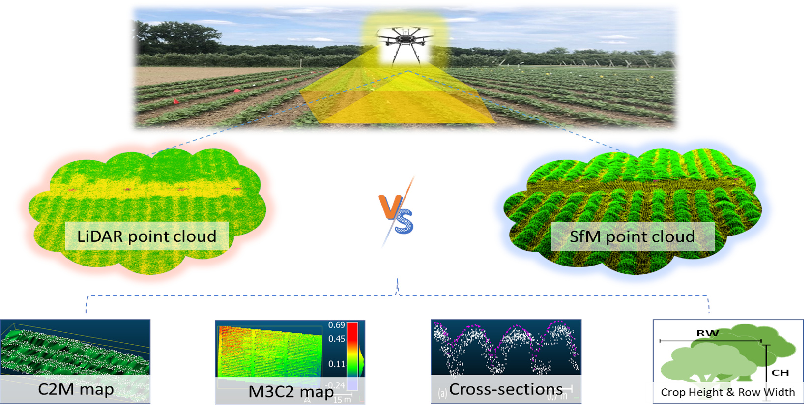
Comparison of UAS-Based Structure-from-Motion and LiDAR for Structural Characterization of Short Broadacre Crops

1
Chester F. Carlson Center for Imaging Science, Rochester Institute of Technology, Rochester, NY 14623, USA
2
Cornell Cooperative Extension, 480 N. Main St., Canandaigua, NY 14424, USA
3
Cornell AgriTech, Plant Pathology & Plant Microbe Section, 15 Castle Creek Dr., Geneva, NY 14456, USA
*
Author to whom correspondence should be addressed.
Remote Sens. 2021, 13(19), 3975; https://doi.org/10.3390/rs13193975
Submission received: 23 August 2021 / Revised: 25 September 2021 / Accepted: 29 September 2021 / Published: 4 October 2021

Abstract

:
The use of small unmanned aerial system (UAS)-based structure-from-motion (SfM; photogrammetry) and LiDAR point clouds has been widely discussed in the remote sensing community. Here, we compared multiple aspects of the SfM and the LiDAR point clouds, collected concurrently in five UAS flights experimental fields of a short crop (snap bean), in order to explore how well the SfM approach performs compared with LiDAR for crop phenotyping. The main methods include calculating the cloud-to-mesh distance (C2M) maps between the preprocessed point clouds, as well as computing a multiscale model-to-model cloud comparison (M3C2) distance maps between the derived digital elevation models (DEMs) and crop height models (CHMs). We also evaluated the crop height and the row width from the CHMs and compared them with field measurements for one of the data sets. Both SfM and LiDAR point clouds achieved an average RMSE of ~0.02 m for crop height and an average RMSE of ~0.05 m for row width. The qualitative and quantitative analyses provided proof that the SfM approach is comparable to LiDAR under the same UAS flight settings. However, its altimetric accuracy largely relied on the number and distribution of the ground control points.

Graphical Abstract

1. Introduction

Unmanned aerial systems/vehicles (UASs/UAVs), paired with structure-from-motion (SfM) image processing workflows, have lately emerged as a popular strategy for various geoscience applications [1,2]. By collecting overlapping image sequences using a high-resolution camera mounted on a UAS and then inputting those images to an SfM algorithm, users effectively can create a three-dimensional (3D) point cloud of a scanned field. Particularly in precision agriculture, the SfM point cloud approach can be used to derive structural parameters of crops, such as plant height [3,4], canopy volume [5,6], and leaf area coverage [7,8], all of which could significantly help farmers to enhance agricultural management decisions [9].
Another widely used approach to generating 3D point clouds is light detection and ranging (LiDAR). LiDAR works by actively emitting high-frequency laser pulses toward the object and recording the reflected responses and transmitted time, from which range measurements can be computed [10]. Over the past decade, LiDAR successfully has been applied in forest inventory as either airborne laser scanners (ALS) [11,12,13] or terrestrial laser scanners (TLS) [14,15,16]. However, as UAS-LiDAR platforms have become more widely used, this approach has proven to be effective and accurate for the structural characterization of shorter vegetation/crops [17,18,19,20]. LiDAR point clouds have obvious advantages when compared with SfM point clouds, including high point density, robustness to illumination changes, and the ability to obtain below-canopy information, because of its multiple return capability from single pulses. However, LiDAR has its own disadvantages: The cost of LiDAR is usually much higher than that of a typical high-resolution color camera used for SfM [6,21]. While SfM algorithms have successfully been integrated into commercial software such as Pix4D, Agisoft Photoscan, or open-source software including OpenDroneMap, the preprocessing of a LiDAR point cloud is relatively more time-consuming and requires more effort, such as trajectory calculation, denoising, point cloud registration, and ground filtering [22,23].
Many studies used LiDAR as a baseline method to evaluate the relative accuracy of SfM point clouds. Some early studies have compared UAS-based SfM point clouds with data collected by TLS [3,4,18,24] and ALS [25,26,27,28]. For example, Holman et al. [3] compared UAS-SfM-modeled wheat plant height with those derived from TLS and field measurement of crop height (CH). Both SfM-derived and TLS-derived models achieve a root mean squared error (RMSE) of 0.03 m. Li et al. [26] used ALS and UAS-SfM point clouds to derive structural metrics of a maize and then used metrics to evaluate the leaf area index (LAI). The results showed that ALS achieve higher accuracy than SfM in evaluating the LAI, with R a d j 2 = 0.85 and r R M S E = 7.16 % versus R a d j 2 = 0.74 and r R M S E = 7.72 % . Such comparisons with TLS and ALS have proved the effectiveness and accuracy of UAS-SfM systems, while highlighting its limitations. However, another important question has yet to be answered: Is a UAS-SfM point cloud as accurate/precise as a LiDAR point cloud under the same flight settings, i.e., when an imaging camera and a LiDAR are installed on the same UAS?
To the best of our knowledge, few studies directly compare UAS-LiDAR point clouds with UAS-SfM point clouds, especially in precision agriculture applications. Cao et al. [29] compared UAS-LiDAR and SfM data in a subtropical coastal planted forest of East China. They found strong correlations (r > 0.9) between metrics such as height percentiles and canopy cover, derived from the two modalities’ point clouds. The two kinds of data, however, were collected on different days and at different flight altitudes (80 m for LiDAR and 500 m for SfM). Lin et al. [30] used a customized UAS-based mobile mapping system to simultaneously collect LiDAR and imagery data over coastal environments. Their results suggested that UAS LiDAR and SfM point clouds are comparable within a 5–10 cm range, and both provided high-resolution and high-quality topographic data. In the context of precision agriculture, Sofonia et al. [31] employed a side-by-side comparison of a Hovermap LiDAR and a RedEdge multispectral camera, mounted on one UAS platform, for monitoring sugarcane growth response. They found that both systems demonstrated similar capabilities for accurate CH measurements ( R a d j 2 = 0.85 0.95 ), while LiDAR provided relatively more consistent and significant correlations. Shendryk et al. [32] predicted biomass in sugarcane using a UAS-based LiDAR and multispectral imagery system. The authors found a similarity between the results of biomass prediction ( R ¯ 2 < 0.57 ) . However, both modalities provided a limited perspective in terms of preliminary comparisons of the point clouds and focused more on the end-level comparisons.
This study focused on the above question and is based on a comparison of UAS-LiDAR and UAS-SfM point clouds, collected at five different growth stages of a snap bean field. Moreover, while most of the previous studies involved relatively high-stature crops, such as rice [33,34], barley [35,36], wheat [3,37], sugarcane [31,32], maize [26,38], and sorghum [39,40], which can grow to be taller than 1–3 m when mature, snap bean represents a short crop that only grows up to 0.6 m at most. It thus can be stated that snap bean results in more stringent requirements when attempting to assess limited vertical-range structural characteristics.
Our study was executed as follows: (i) First, we preprocessed and geospatially registered LiDAR and SfM point clouds; we estimated the primitive absolute accuracies of the checkpoints in both point clouds by utilizing the recordings of ground control points (GCPs); (ii) we then directly compared the two kinds of point clouds in terms of a point density map, histograms of z coordinates, and SfM point cloud to LiDAR-derived mesh (cloud-to-mesh (C2M)) distance maps; (iii) after implementing rasterization and interpolation on the point clouds, we next compared their derived products, including digital elevation models (DEMs) and crop height models (CHMs), by calculating the difference of the models and the multiscale model-to-model cloud comparison (M3C2) distance; (iv) as a complement to the above comparisons, we made qualitative comparisons between the cross-sections of the two point clouds; (v) finally, we compared the CH and row width (RW) of sampled rows, derived from both point clouds, with in-situ measurements in one of the data sets. Based on all the analyses above, we hope to provide a definitive comparison of UAS-based SfM vs. LiDAR point clouds in the context of the structural characterization of short broadacre crops, with snap bean being our proxy crop.

2. Materials and Methods

In this section, we first introduced the study site and the collected data (Section 2.1). We then explained the data processing steps (Section 2.2), followed by details on the methods and evaluation metrics that were applied to compare the data derived from the LiDAR and SfM approaches (Section 2.3).

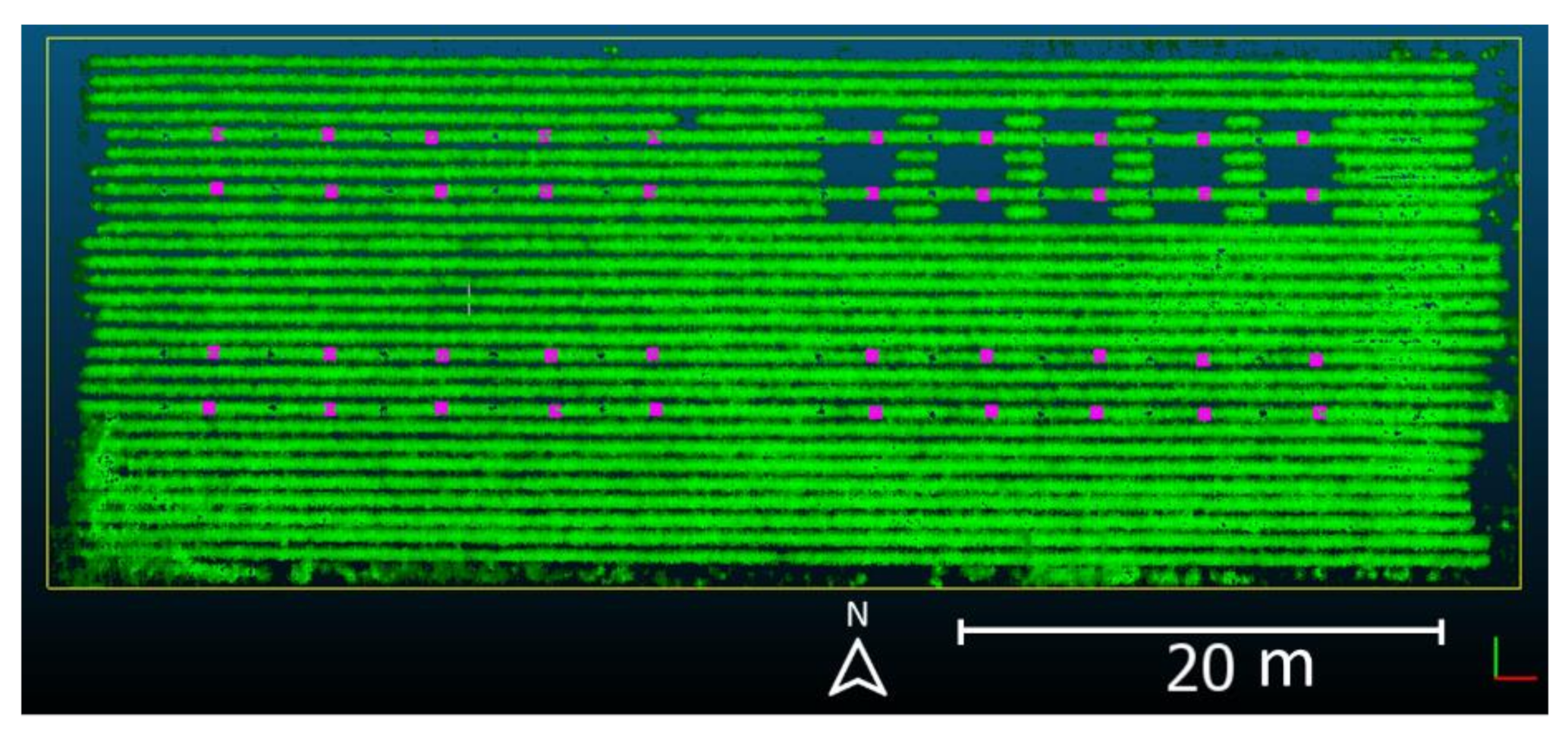
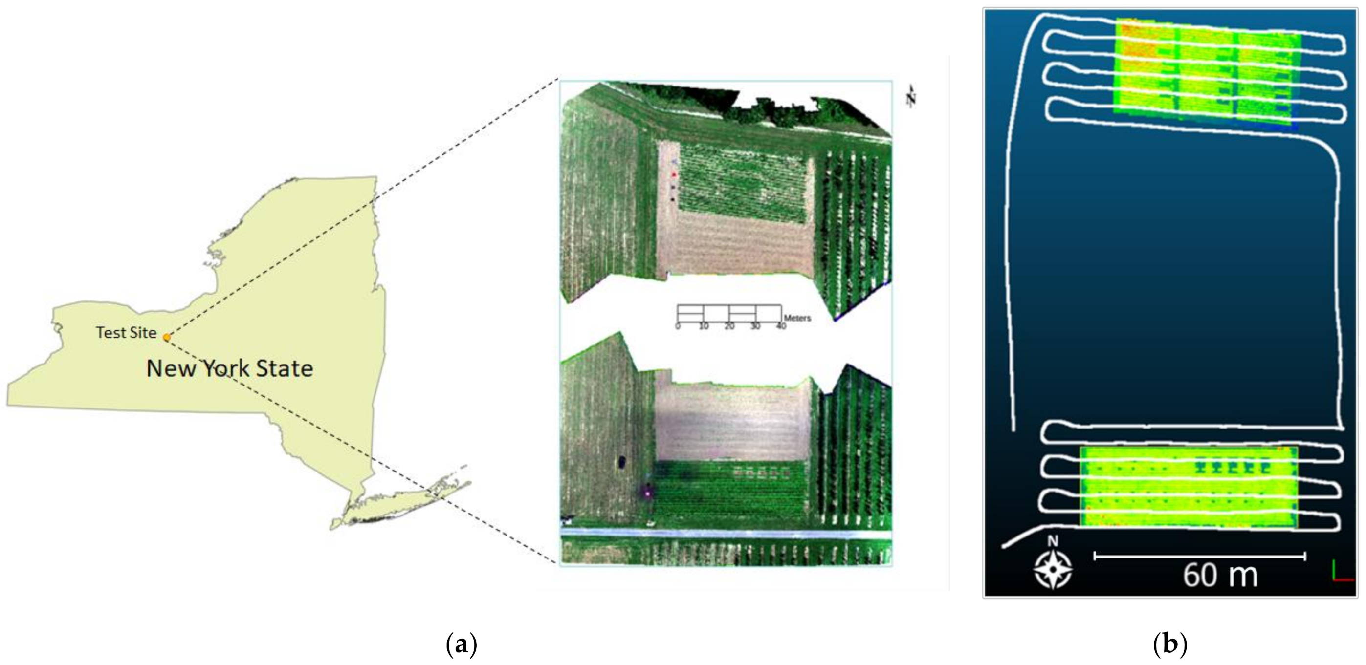
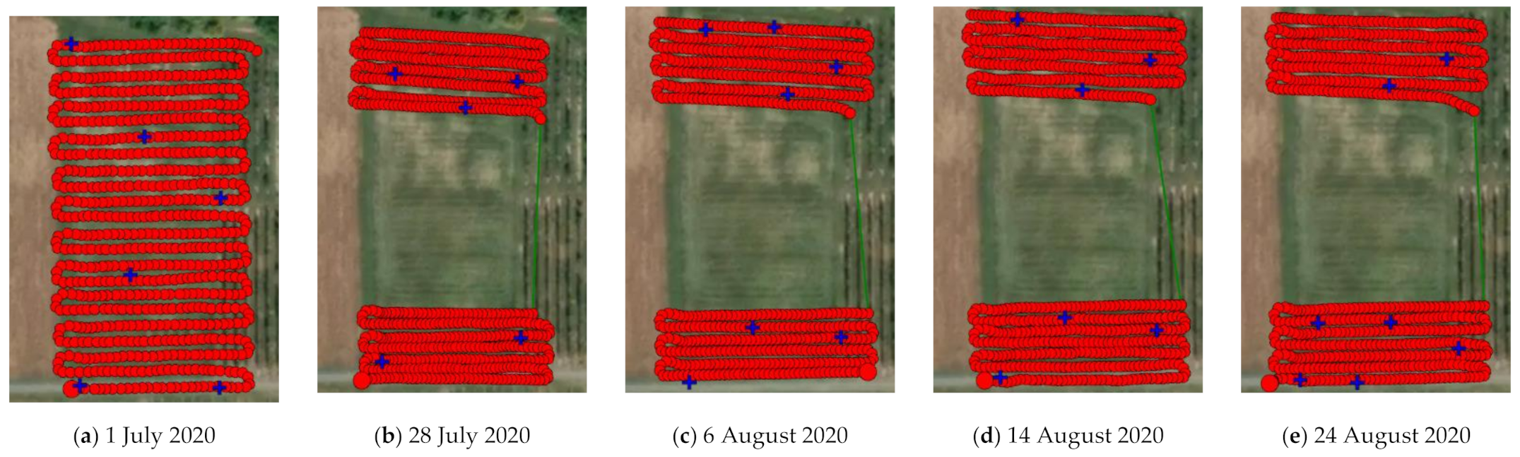
2.1. Study Site and Data Collection

Our study site is located in Geneva, NY, USA (42°52′0.00″ N, 77° 1′43.00″ W; Figure 1a). The field consisted of two plots that were 100 m apart in the north–south direction. The north plot had three replications of six snap bean cultivars: Venture, Huntington, Colter, Cabot, Flavor Sweet, and Blevet. Each cultivar in each replication had four rows, resulting in 72 rows in total. The south plot contained only the Huntington cultivar, with 40 row segments treated as experimental plants and half of them inoculated with white mold after the first flowering stage. The sizes of the two plots were 1512 and 1416 m2, respectively (Figure 1a).
The UAS system used a DJI Matrice 600 Pro hexacopter as a base platform. It consisted of a global navigation satellite system (GNSS)/inertial measurement unit (IMU; Trimble APX-15 UAS V2), a Velodyne VLP-16 PuckTM LiDAR (Velodyne, San Jose, CA, USA), and a MicaSense RedEdgeTM multispectral camera (MicaSense, Seattle, WA, USA). The GNSS/IMU unit provided recordings of the geolocation and the GPS time during flights. The VLP-16 LiDAR generated up to ~600,000 points/second in a dual return mode. It operated in a 360° horizontal field of view and a ±15° vertical field of view. The claimed range accuracy was ±3 cm, and the laser wavelength was 903 nm. The MicaSense RedEdge captured images of five spectral bands: blue, green, red, red edge, and near-infrared, centered at 475, 560, 668, 717, and 842 nm, respectively. We implemented five flights across five days to collect data on the snap bean crop at different growth stages. Figure 1b shows an example of the flight trajectory, along with a LiDAR point cloud. The flight information and the data set specifications are listed in Table 1. For data set #3, we took ground measurements of the CH and the RW by sampling three times per row in the northern plot and two times per row segment in the southern plot by using a measuring tape.

2.2. Processing of the UAS-Based 3D Point Cloud Data

The processing of the SfM and LiDAR point clouds mainly included three steps: (1) preparing the data for comparison (data preprocessing); (2) deriving gridded models from the point clouds, including DEMs, digital surface models (DSMs), and CHMs; and (3) extracting segments of the vegetation points, calculating the CH and the RW and comparing them with ground measurements.

2.2.1. SfM and LiDAR Point Cloud Preprocessing

We input the multispectral images to a Pix4Dmapper (v.4.6.4, Pix4D S.A., Prilly, Switzerland) to generate SfM point clouds. While we mostly used it as an end-to-end tool, the basic principles of the SfM algorithm have been well-explained in previous studies [1,31,41,42]. First, the algorithm computes the keypoints and descriptors for all the images toward automatic image matching. In this step, at least 75% cross-track and along-track overlapping is recommended for the Micasense RedEdge camera [43] to ensure enough common features are identified. The algorithm next applies a bundle adjustment and a 3D scene reconstruction to generate a sparse point cloud, which then is densified to create a dense point cloud. The GCPs next are imported to georeference the point cloud. In our study, we used AeroPointsTM (Propeller, NSW, Australia) checkerboards as GCPs and evenly distributed them in the field during the flights. With a proper set-up, the global accuracy of the GCPs is claimed to be 10 mm + 1 ppm horizontally and 20 mm + 1 ppm vertically [44].
The SfM point cloud preprocessing was quite direct—we visualized the SfM point cloud in the software CloudCompare (v.2.12 alpha [45]) and cropped it spatially to valid scene extents by the manual image interpretation of the field color patterns. However, it is worth noting that in our study, the default georeferencing system (NAD 83/NAVD 88) for the AeroPoints was different from that of the APX-15 (WGS 84/EGM 96), which was used in generating coordinates for the LiDAR point clouds, while the essence of the z coordinates also differed. In AeroPoints, it implies the orthometric height (height above geoid), while in APX-15, it refers to the ellipsoidal height (height above ellipsoid). For example, the difference between the ellipsoidal and the orthometric height was −35.00 m at the location of our study site in the WGS 84/EGM 96 geographic coordinate system. We therefore converted the recording of the GCPs’ coordinates using the software VDatum (v.4.0.1, NOAA, Washington, DC, USA [46]) to geospatially register the SfM point clouds with the LiDAR point clouds.
The preprocessing of LiDAR point clouds included a few more steps: (1) retrieving the flight trajectory from the IMU file, which focused on the transformation of geographical coordinate and time units; (2) temporal and spatial cropping according to field boundaries and flight trajectories; (3) removing outliers and noise using a statistical outlier removal (SOR) filter; (4) removing second return points and duplicate points; and (5) computing the scan angles of the points by using the IMU flight trajectory; and then filtering out the points with large scan angles (>20°), which theoretically had larger errors. Our LiDAR data preprocessing steps were similar to those by Sofonia et al. [47], except that in step 4, we did not need the second return points. This was because the VLP-16 LiDAR can only distinguish between two returns per pulse when the distance between the two returns is >1 m [48], while the heights of all the snap bean plants are <1 m. We filtered the points with too large scan angles in step 5, since larger scan angles resulted in the increased off-nadir distances of the laser beams, thus leading to significant errors, due to the footprint size of a laser beam increasing at the square of the transmitting distance. For steps 2–4, we used LAStools [49] and CloudCompare; for steps 1 and 5, we used Python 3 programming.

2.2.2. Derivation of Digital Models

As many previous UAS-based studies proposed [50,51,52], the derivation of the CHM involves deriving the DEM and the DSM, which was calculated as:
CHM   =   DSM     DEM .
The DEMs were generated from the preprocessed SfM and LiDAR point clouds from data set #1, which was collected when the field contained only bare ground (Table 1). We set the grid spacing of the DEMs to 0.05 m, similar to the study of Lin and Habib [20]. We chose this value due to the following reasons: (1) it is small enough to retain plant structural details, and (2) it is large enough to ensure that most cells would include more than one point, i.e., cell values could be decided using actual data, instead of interpolation. For both the SfM and LiDAR point clouds, we first rasterized them based on point clouds with a regular spacing, by calculating the average z value in each cell. We then filled the empty cells using ordinary kriging interpolation in Surfer (v.15.3.307, Golden, CO, USA). We derived the DSMs from data sets #2–5 using rasterization and interpolation, such as the DEM generation process except for one difference—in rasterization, we used the highest z value, instead of the average value as the representative for each cell. Finally, we computed the CHMs using Equation (1).

2.2.3. Calculating CH and RW from Vegetation Sample Points

To evaluate the relative accuracy of the SfM-derived and LiDAR-derived CHMs, we calculated the CH and the RW from row segments in the CHMs from data set #3 and compared them with ground measurements. The extraction of segments of vegetation points is shown in Figure 2. We filtered out all the points with a height lower than 10 cm to ensure ground points did not impact the calculation. Within each segment, we calculated CH by finding an optimized top percentile of the z values. Similarly, we calculated the RW by finding an optimized difference between a well-above average percentile and a well-below average percentile of y values. The optimal values were determined by finding the smallest RMSE between the derived metrics and the field measurements [23]. Specifically for the north plot, since the original direction of the rows were at an angle of 6.6 ° due east (measured in CloudCompare), we manually applied a rigid transformation to rotate the point clouds to make the rows horizontal.

2.3. Comparing Methods and Evaluation Metrics

The sparsity and non-uniform point density of 3D point clouds introduce a level of complexity, which necessitates a multi-pronged approach to assessing the data quality. We thus evaluated the characteristics of the UAS-based SfM and LiDAR point clouds during different processing stages. We first made preliminary comparisons among the “raw” data, such as the accuracy of GCPs’ centers, average density, and z-histograms. We then compared the preprocessed point clouds and their derived DEMs and CHMs. After that, we observed the cross-sections (side-view) of small segment samples in the preprocessed point clouds versus the CHMs in data set #3, to serve as a complement to the previous top-view comparisons. Finally, we selected data set #3 to compare the CH and the RW, derived from the CHMs, with ground measurements.

2.3.1. Preliminary Comparisons

The distribution of the valid GCPs for each data set is shown in Figure 3. In fact, we placed nine GCPs in the field during all flights, although a couple of them failed to operate properly due to equipment aging. Similar to Lin and Habib [20], the absolute accuracy of the SfM and LiDAR point clouds was assessed against the AeroPoints recordings of the GCPs deployed at the site. We manually identified them based on the patterns, in order to determine the coordinates of the center of AeroPoints GCPs from an SfM point cloud. Due to the uncertainty of the LiDAR detection range, the determination of the GCP centers in the LiDAR point cloud required a more complex strategy. LiDAR points of a planar panel had a significant vertical variance and exhibited “multiple layers” as opposed to the “single-layer” counterpart in an SfM point cloud. We applied the approach proposed in Lin and Habib [20] to identify the centers: (1) manually selecting initial centers based on the intensity patterns; (2) finding all points that lay within a spherical neighborhood with a radius of 0.25 m and are centered at the initial points; and (3) fitting a plane among the neighboring points and then projecting the initial points to the fitted plane. The projection points on the fitted planes were finally identified as the GCP centers from the LiDAR point clouds. It should be noted that we selected 0.25 m as the radius in step (2), because this radius ensured that all the points within the neighborhood were from the checkerboard, given that an AeroPoints GCP’s dimensions are 0.544 m × 0.544 m. Finally, we compared the average surface point densities of the SfM point clouds and LiDAR point clouds in all data sets and the histograms of their z coordinates.
Finally, we also calculated the average surface point densities and the histograms of z-coordinates for each data set.

2.3.2. Derived Products Comparison

Four point cloud comparison methods are commonly used to compare 3D point clouds: DEM of difference (DoD) [53,54,55,56], cloud-to-cloud (C2C) distance [57,58,59,60], C2M distance [47,61,62,63], and M3C2 distance [64,65,66,67,68,69]. The DoD approach subtracts two DEMs or DSMs using a top view and is fast/easy to implement and interpret. However, the disadvantages are that it requires gridded representation, only estimates vertical distance and is sensitive to errors caused by misregistration [70]. In the C2C approach, two point clouds are set as the reference point cloud and the compared point cloud, respectively. For each point in the compared point cloud, the closest point can be determined in the comparison point cloud. This is the fastest and simplest 3D comparison method [64]. The measured distance can be assessed as the x/y/z directions but is sensitive to the cloud roughness, outliers, and point spacing [68]. As the SfM point cloud had a significantly lower point density than the LiDAR point cloud, it resulted in a larger point spacing for the former. The DoD and C2C methods were not suitable for a direct comparison between the two modalities, so the C2M approach was used for a robust comparison.
We used CloudCompare to calculate the C2M distance between the SfM and LiDAR point cloud-generated meshes. First, a mesh was generated using the Delaunay 2.5 D (best fitting plane) mesh tool from the LiDAR point cloud. Then, a C2M distance map was computed for the SfM point clouds, relative to the LiDAR-generated meshes. The output was saved as a scalar field in the SfM point clouds. Thus, the point density difference between the two types of point clouds did not impact the results.
The M3C2 is a relatively recent 3D comparison approach that calculates both distances and uncertainties [64]. It has advantages: (1) taking into account local normals, roughness, and registration errors, (2) allowing direct application to two un-rasterized point clouds (although it is still not ideal for the direct comparison of SfM with LiDAR, since SfM point clouds have a much lower density and even empty holes), and (3) resulting in distance calculations on the normal directions [64,68]. Therefore, we used the M3C2 to compare the derived digital models (DEMs and CHMs) from the point clouds. The algorithm includes four main steps:
  • Find the “core” points, which are essentially a sub-sampled version from the original point cloud;
  • For each core point, a normal vector is defined by fitting a plane to its neighbors, enclosed by a user-defined diameter D , which is named “normal scale”;
  • Given every core point and its normal vector, a cylinder can be defined via the user-defined projection scale, d , and the cylinder depth, h , oriented along the normal direction. Thus, the intercept of the two clouds with the cylinder defines two subsets of points; and
  • Project both subsets to the orientation axis of the cylinder, i.e., the normal vector, to generate two distributions of distances. The distance between the means or medians of the two distributions is the local distance, L M 3 C 2 .
We used CloudCompare to implement the M3C2 in our study. Apart from the L M 3 C 2 distance map, CloudCompare also provided two more outputs: the distance uncertainty map and the change significance map. The distance uncertainty measure (at a level-of-detection of 95%, i.e., L 95 % ) was calculated by:
L 95 % = ± 1.96 σ 1 d 2 n 1 + σ 2 d 2 n 2 + r ,
where σ 1 and σ 2 are the variances of point positions for each subset in step 3, n 1 and n 2 are the number of points in the subsets, and r is the co-registration error between two point clouds. These parameters are determined locally by the algorithm itself. The change significance map consists of binary values that indicate whether the distance corresponds to a real change or not [71].
As described above, three key parameters, namely the projection scale ( d ), the cylinder depth ( h ) , and the normal scale ( D ), need to be manually defined. We set d as 0.15 m, because the point spacings for the DEMs and the CHMs were 0.05 m and thus at least six points would be included in each sub-cloud, which was more than the four points required by the M3C2 algorithm [65]. Considering the scale of snap bean—CH (up to ~0.65 m) and RW (up to ~0.70 m), we set h = 0.80 m, so that when the normals were calculated on one side of a row, the cylinder in each local neighborhood was large enough to enclose sufficient points and small enough not to enclose unwanted points from the other side of the row. Previous research based on landslide [66], open-pit mines [65], and canyon studies [64] generally set D as 20–25 times the average roughness in each point cloud. However, in our application, when D varied from 0.15 to 0.30 m, the average roughness of the digital models ranged from 0.01 to 0.03 m, i.e., D were 10–15 times the roughness. Based on our preliminary knowledge of snap bean crops, we considered the size of the snap beans as also limiting the value of D. More specifically, a proper D should fall within 0.15–0.40 m, so that abundant points can be included to calculate the normals and to ensure that the normals reflect the genuine local features of the crops. We therefore fixed the normal scale D at 0.30 m, which was twice the projection scale ( d ), a ratio that was close to the settings used in the aforementioned studies [64,65,66,68].
We used three standard accuracy measures to evaluate the differences calculated by C2M and M3C2 approaches, namely the mean difference (MD), the standard deviation of the difference (St. Dev), and the RMSE.

3. Results

3.1. Preliminary Comparison of the Point Clouds

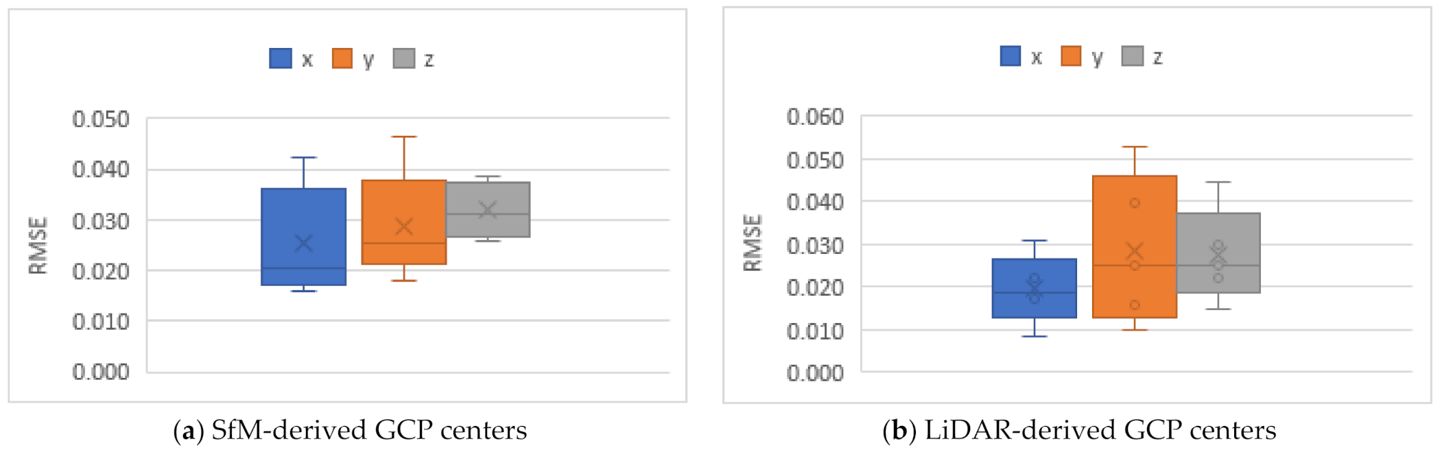
3.1.1. Absolute Accuracy of GCPs

Figure 4 shows the box and whisker plots of the RMSEs of the differences between the 3D point cloud-derived coordinates of the GCPs centers against the AeroPoints measurements. The results included all the GCPs in the five data sets. We found that for both SfM and LiDAR point clouds, the average uncertainties (RMSE) in the x/y/z directions were about 0.01–0.03 m. Thus, both SfM and LiDAR point clouds achieved high accuracies.

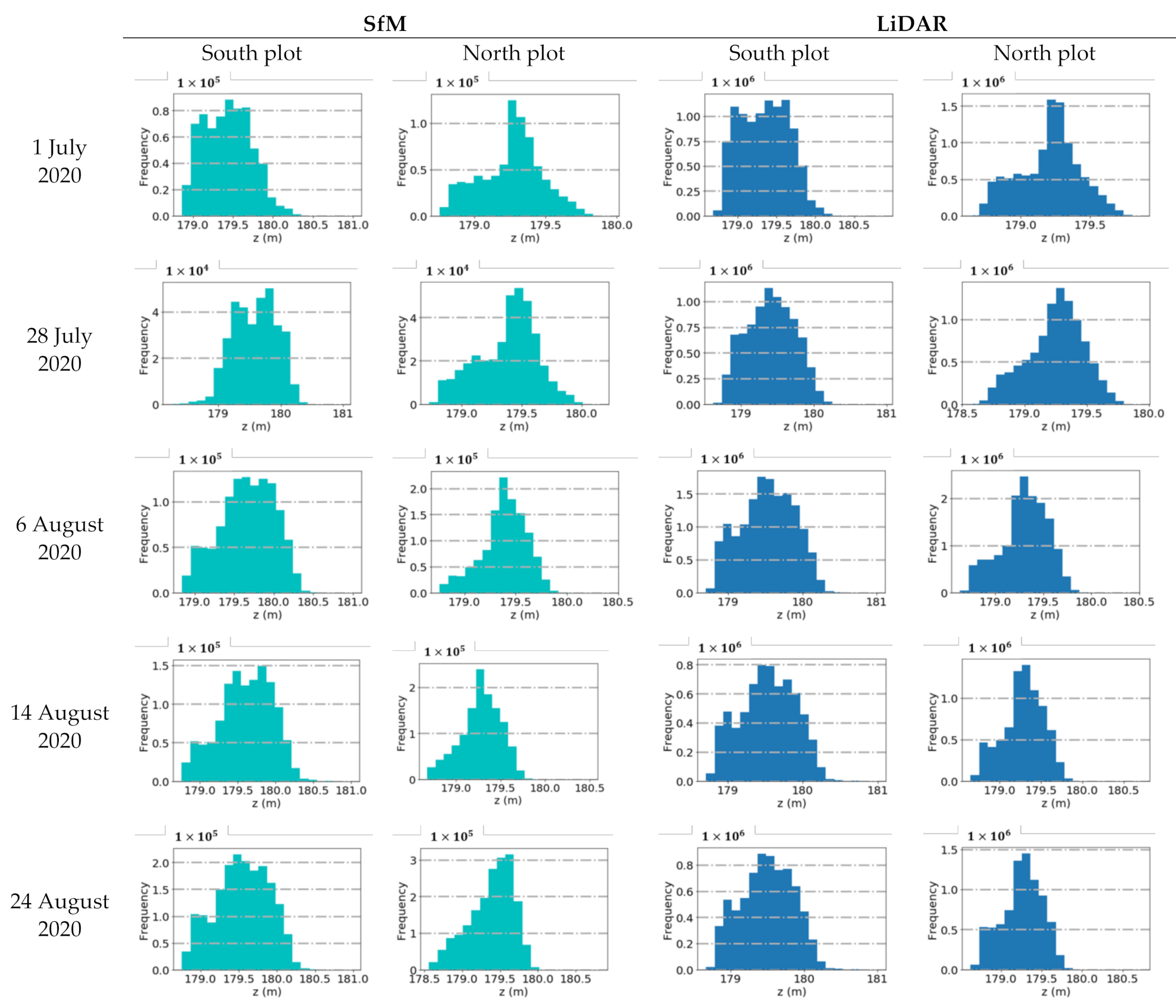
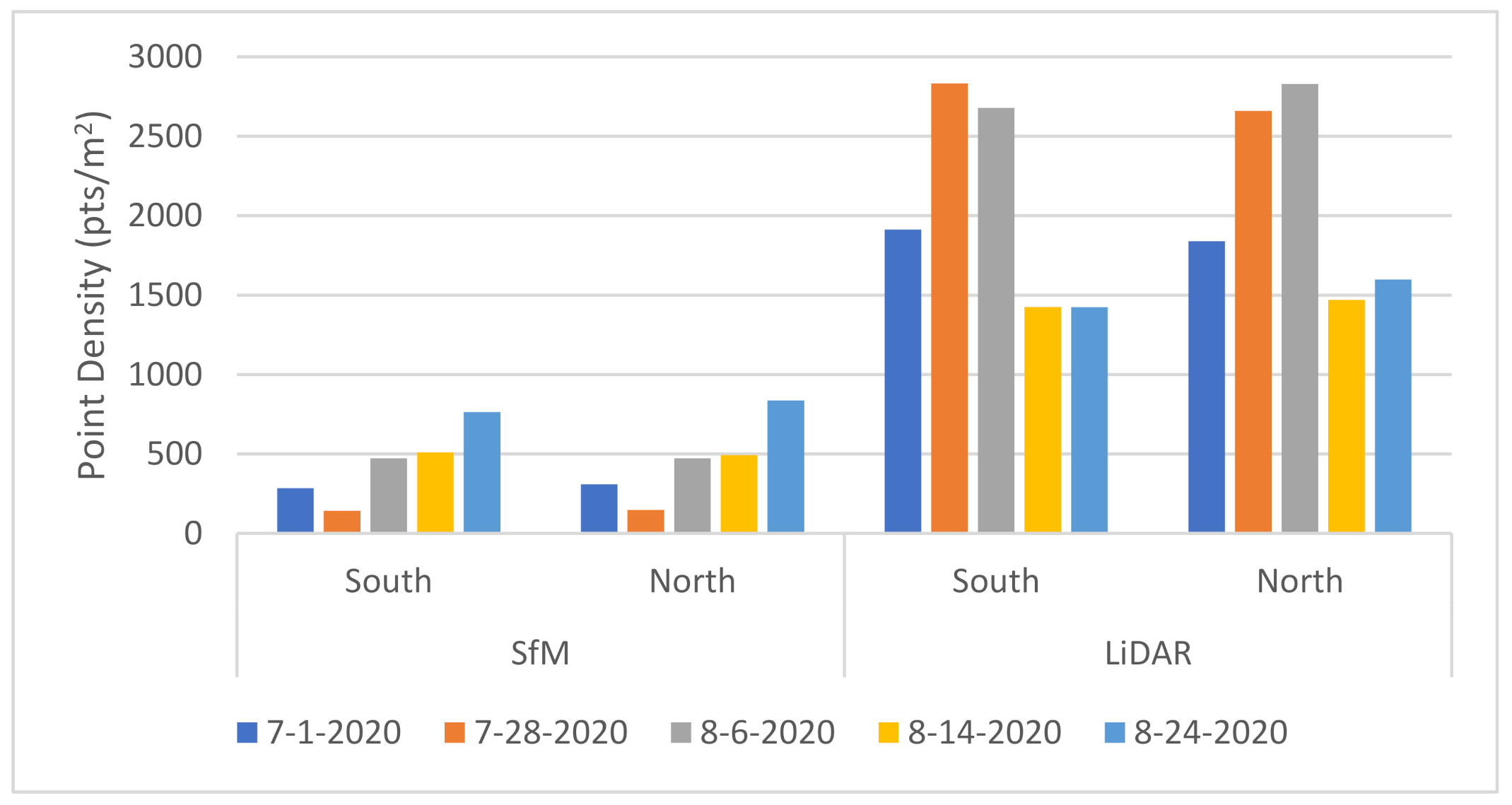
3.1.2. Average Density and Histograms of the z Coordinate

The average point densities of each SfM point cloud and each LiDAR point cloud are shown in Figure 5. The SfM point density ranged between 140 and 840 pts/m2, while the LiDAR point density ranged between 1400 and 2800 pts/m2. It was not surprising that the point densities of both plots had a slight difference, since the data of the south plot and the north plot were collected during the same flights, with the same flight altitude, flight speed, flight line space, and even number of flight lines. This furthermore proved that, despite the difference of the snap bean variabilities in the two plots, the surface point density was mainly determined by the flight settings.
Figure 6 shows the histograms of all the point clouds. We found that SfM and LiDAR had similar distributions of bins for all data sets. The south plot histograms were more symmetric than the north plot histograms, while the latter usually had a long tail (more bins of small z-values). This was attributed to the south plot containing only one snap bean cultivar; these single-cultivar plants grew more uniformly than in the north plot, which had six cultivars. By comparing the first column with the third column, we observed that the bins of the small values in the LiDAR histograms were higher than in the SfM histograms, which indicated that more near-ground information was retained. This was likely due to the low-altitude points originating from stems near the ground and below leaves; LiDAR could actively scan them when its beam hit the stems at the right off-nadir angle, while the SfM point cloud was generated “passively” from imagery, on which the stems tended to show up as unlit/dim pixels, given that they were either in shadow or visually fully occluded.

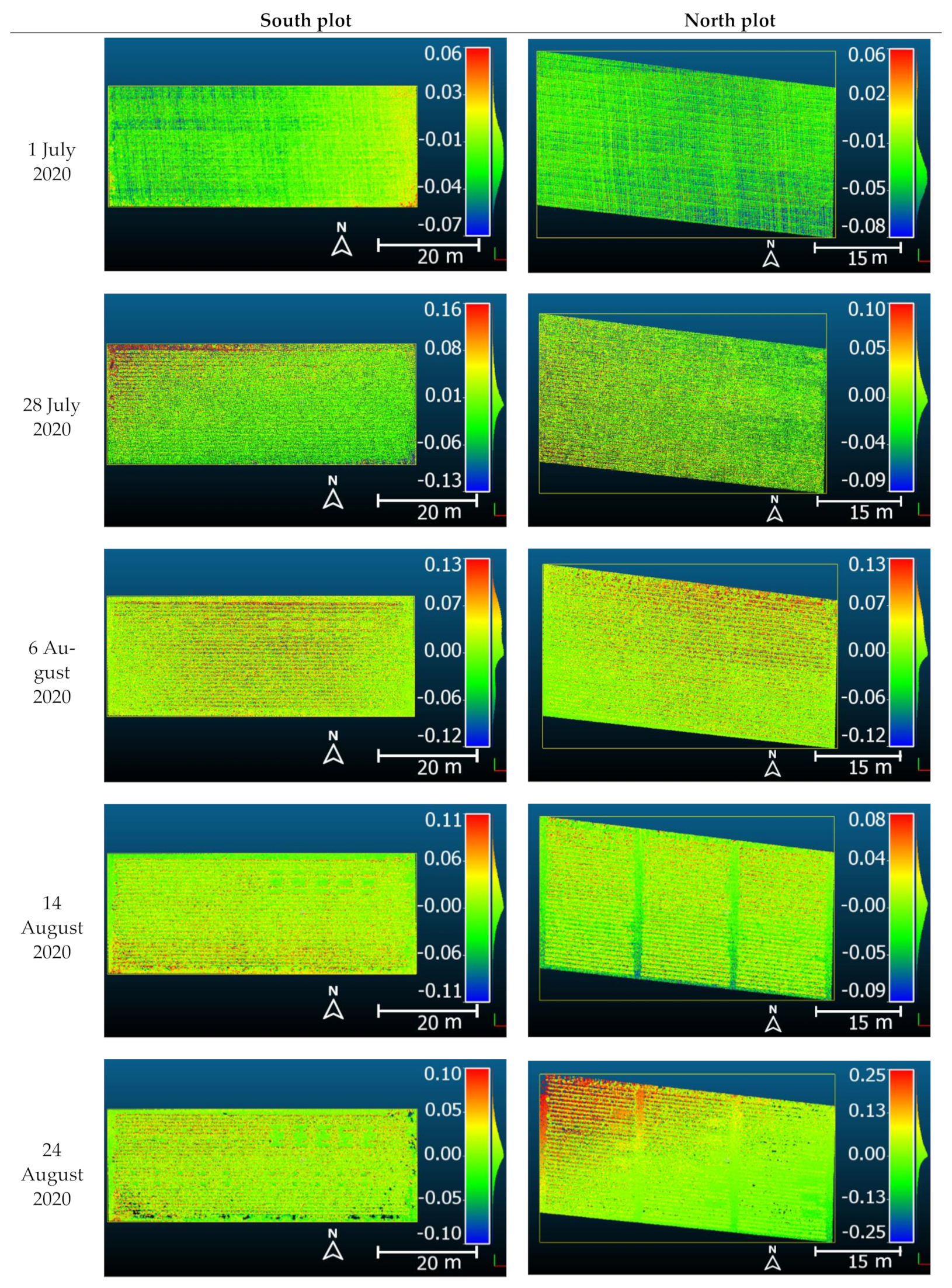
3.2. C2M Distance Map Derived from the Preprocessed Point Clouds

The C2M distance maps were computed for both the north and south plots for all data sets (Figure 7). We found that the errors from the vegetation points were generally greater than those from the ground points. Most of the C2M maps exhibited uniformly distributed differences over the whole plot, except for the south plot on 28 July 2020 and the north plot on 24 August 2020; both dates presented relatively more significant errors in the top left corner. This was attributed to the unevenly distributed valid GCPs on these two dates (Figure 3), i.e., there was no valid GCP near those corners. Table 2 shows the statistics of the C2M maps. Most of the differences were below 0.05 m (RMSE = 0.03–0.05 m), except for the north plot in the last data set (RMSE = 0.08 m).

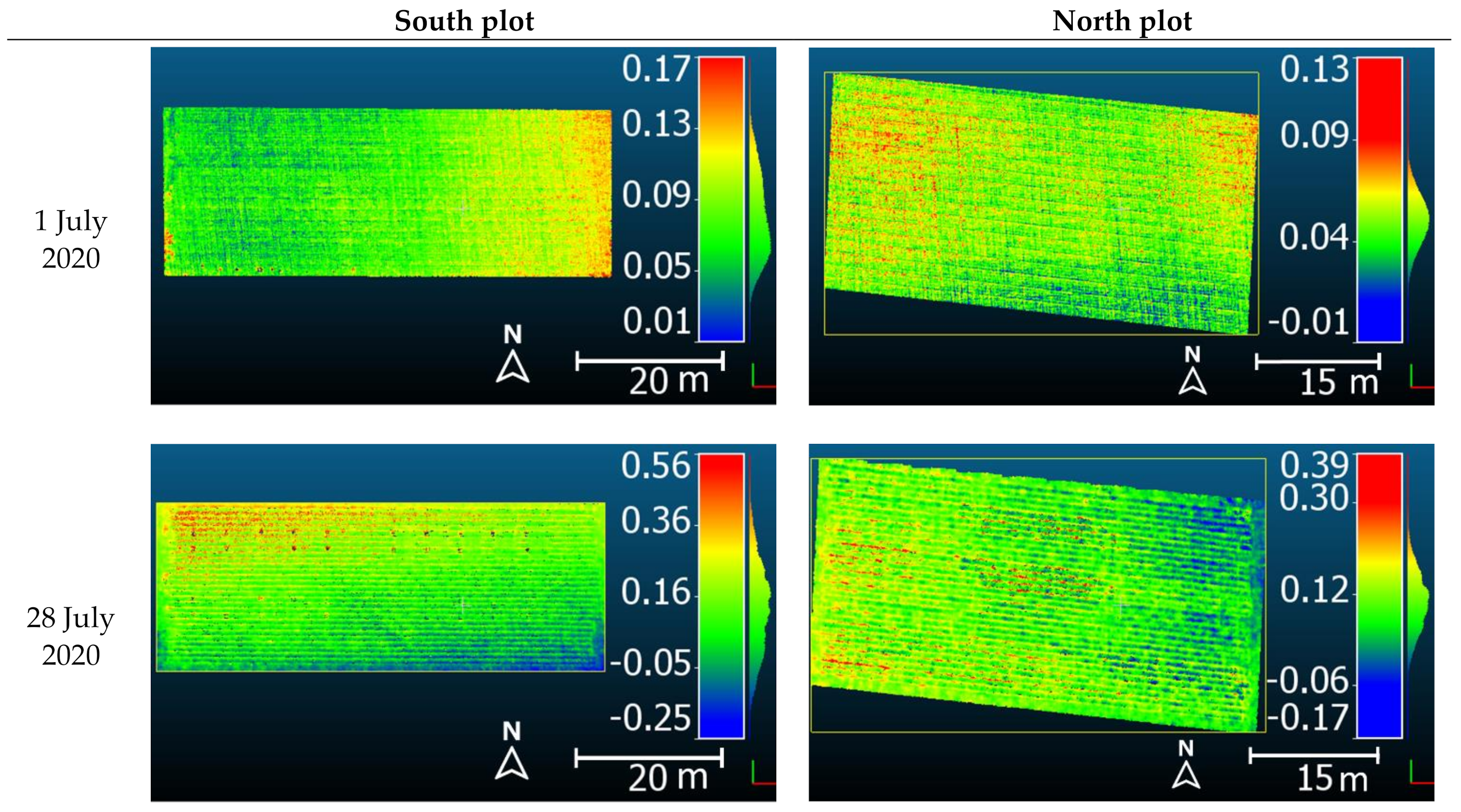
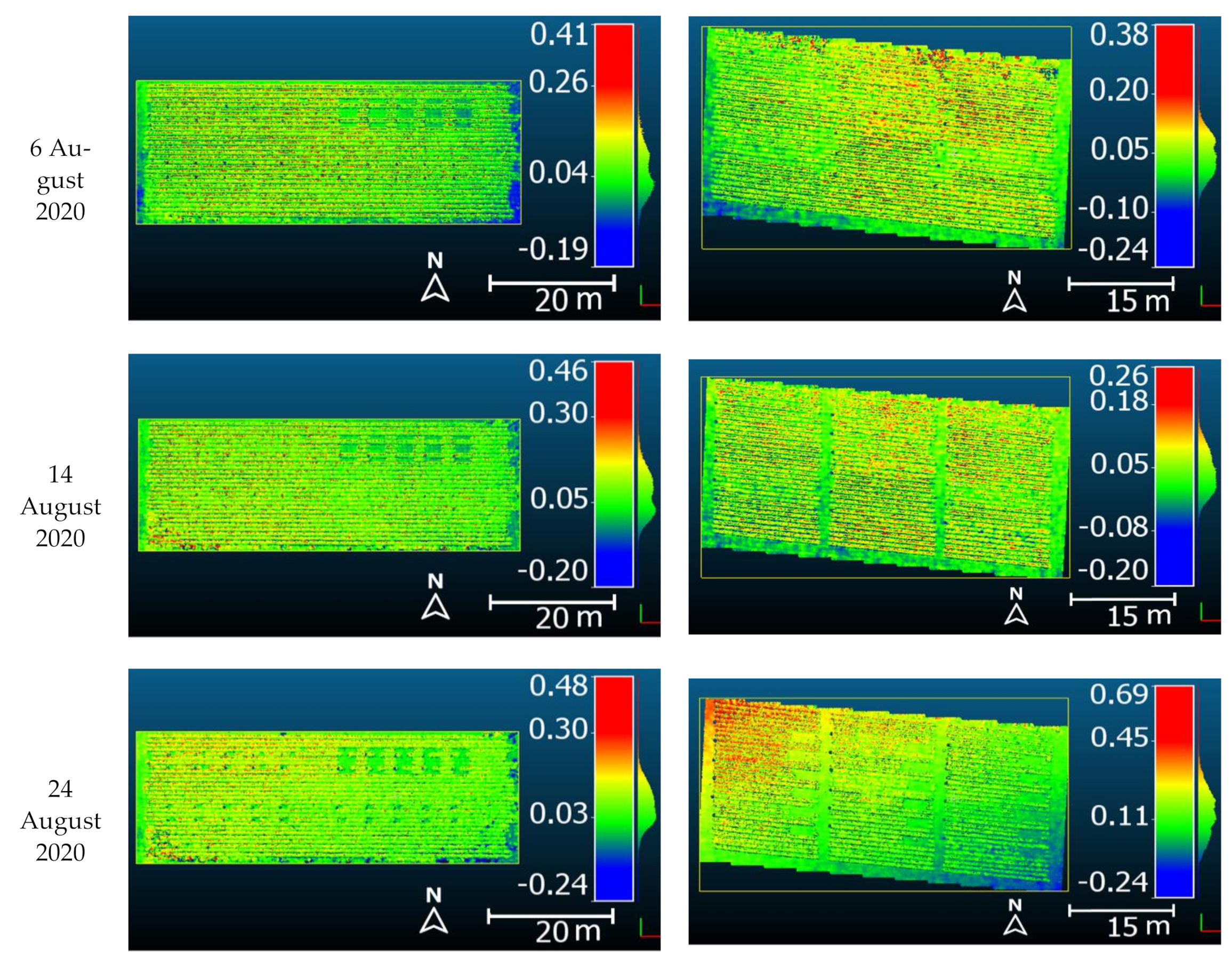
3.3. M3C2 Distance Map Derived from the DEMs and the CHMs

The results of the M3C2 maps are shown in Figure 8. We eliminated the outlier points with significant uncertainties (above 0.15 m) and large absolute errors (far beyond the prominent peak of the histogram). The remainder of the points are shown below. Table 3 shows the statistical metrics of the M3C2 distance maps. By comparing Figure 8 with Figure 7, we found that the M3C2 maps better reflected the spatial distribution of the differences than the C2M maps by providing the following: (1) stronger contrast between warmer colors (taller) and colder colors (shorter); and (2) distance histograms that exhibited larger ranges. Table 3 shows that, except for the data sets from 28 July 2020 to 24 August 2020, which exhibited large errors/differences (RMSE = 0.10–0.18 m), the other three data sets showed distance differences ranging between 0.05 and 0.10 m.

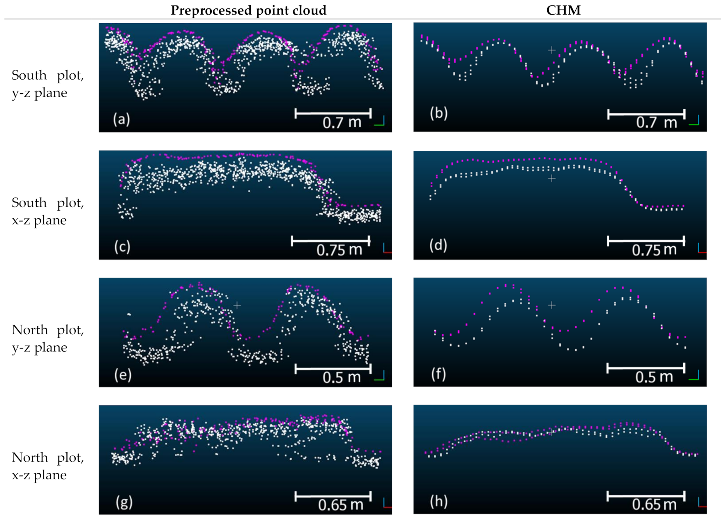
3.4. Comparison of Sampled Cross-Sections in Point Clouds

We extracted two types of cross-sections by segmenting out thin slices of points across rows (Figure 9a,b,e,f) and along a row (Figure 9c,d,g,h) from a top-down view; this was performed, since the snap bean field exhibited repetitive patterns. The SfM point cloud was a “single-layer” point cloud that envelopes the snap bean plants, while the LiDAR point cloud presented “multiple layers” with much denser points in the 3D space. Although both point clouds could detect the snap bean rows and alleys (bare ground area between rows), the LiDAR point clouds retained more detail of the valleys than did the SfM point clouds. The SfM point clouds were generally higher than the LiDAR point clouds, and so were the derived CHMs. By comparing the left column (Figure 9a,c,e,g) with the right column (Figure 9b,d,f,h), we also observed that the CHM models did provide a clearer view of the geometric shape of the field.

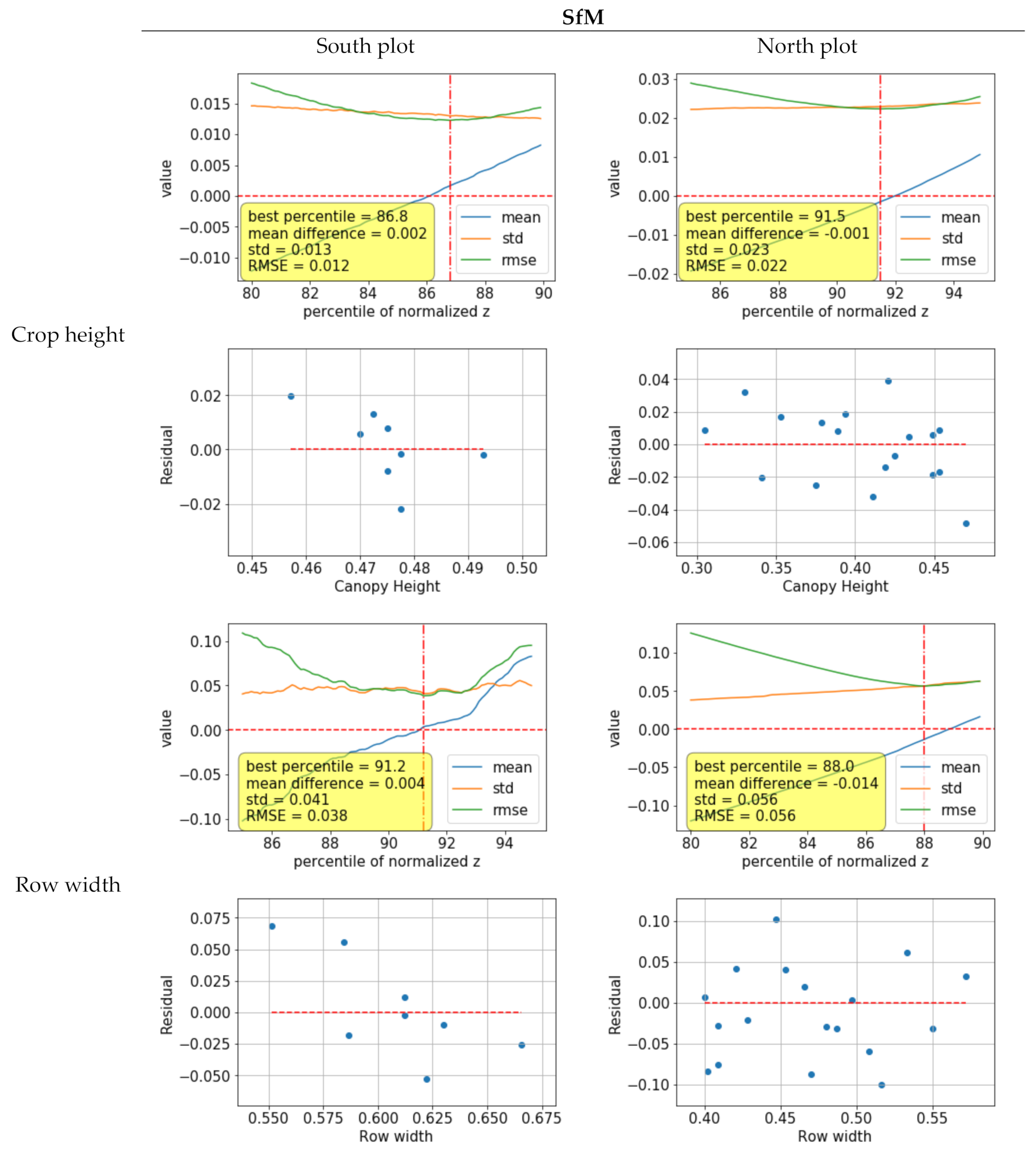
3.5. Comparison of the Sampled CH and RW

As described in Section 2.2.3, different top percentiles of z-values resulted in different predictions of CH and thus yielded different errors when compared to ground truth measurements. The same was true for the central percentiles of y-values in terms of RW. Figure 10 shows the absolute errors of the predicted CH and RW from the SfM-CHM versus the corresponding ground measurements in data set #3, as per different percentiles. We could find the best SfM results by locating the percentile, which generated the lowest RMSE, by observing the curves of the RMSE vs. percentile. We applied the same approach to the LiDAR point clouds and obtained the statistical metrics listed in Table 4. We found that the errors for the north plot, which had a larger cultivar variety, were larger than those for the south plot. For both point clouds, the CH calculation turned out to be more accurate than the RW calculation. We found that the SfM approach matched LiDAR as modality and even performed slightly better when evaluating CH, by comparing the RMSEs from both SfM and LiDAR. The 0.1 interval on the x-axis resulted in the curves for the SfM approach “oscillating” more obviously than those from LiDAR. This was attributed to the fact that many points in the SfM CHM were generated by interpolation, while most of the points in the LiDAR CHM were generated by selecting representative samples among real points. In LiDAR-CHMs, the best top percentile of z-values for calculating CH was 98.8 % ± 0.4 % , and for calculating RW, it was 95.7 % ± 0 ; for the SfM-CHMs, the best central percentile of y-values for calculating CH was 89.2 % ± 2.4 % , and that for calculating RW was 89.6 % ± 1.6 % .

4. Discussion

4.1. Qualitative and Quantitative Comparisons of the Two Modalities

The qualitative comparison between the SfM and LiDAR point clouds in our study included observations of the z-histograms, the C2M distance maps, the M3C2 distance map, and the cross-sections projected on two vertical planes. Each of the methods included results from both the north plot and the south plot in the field. We concluded that the differences between the two kinds of point clouds were not discernable in the z-histograms and were slight in the C2M distance maps. The M3C2 approach, in contrast, which calculates the difference in normal directions, revealed more obvious spatial variability.
Most parallel studies that used the M3C2 algorithm to compare UAS-SfM with LiDAR were in geomorphological applications, and their LiDAR systems varied. Cook [72] compared the UAS-SfM point cloud of a bedrock gorge with terrestrial LiDAR data during the same survey period using the M3C2 algorithm. While the dominant GSD was ~1.8–2.6 cm, the author reported an RMSE of 0.3–0.4 m; however, that study also found that that the SfM accuracy varied by different surface features, with vegetation, water, and other textures causing more errors. Bash et al. [73] analyzed the precision and accuracy of a UAS SfM point cloud versus airborne LiDAR data over a spring snow surface at Haig Glacier; with a GSD of 2.4 cm, most of the errors were within a range of 0.049 ± 0.111 m. Our M3C2 distance between UAS-based LiDAR and SfM point clouds resulted in distance RMSEs of 0.05–0.18 m, which seemed to be slightly better than those from previous studies. However, this also could be attributed to the smaller GSD of 0.017 m in our study, while our study field only contained vegetation and ground surfaces, which were relatively more homogeneous than the sites from previous studies.
From the SfM point cloud in data set #3, we obtained RMSEs of 0.01 m and 0.02 m by directly comparing the calculated CH with the observations of the south plot and the north plot, respectively. The accuracies (in terms of the scales of RMSE and the relative RMSE) surpassed many related studies. Becirevic et al. [69] tested the effectiveness of UAS-based SfM point clouds for measuring the CH of winter wheat (up to 1 m when mature) and obtained an RMSE of 0.022 m in a linear regression model between the observed and calculated values. De Souza et al. [51] evaluated the CH of sugarcane (up to 3.2 m when mature) using SfM point clouds generated on a fixed-wing UAS platform and reported an RMSE of 0.40 m. Chang et al. [50], in turn, monitored the CH of sorghum (Sorghum bicolor; grew up to 2.7 m) using an SfM point cloud and achieved an RMSE of 0.33 m. Finally, Ziliani et al. [18] compared the CH of a maize (up to 2 m when mature), derived from fixed-wing UAS-based SfM point clouds, with corresponding field measurements and obtained an RMSE of 0.21 m during the flowering growth stage. This was corroborated by Chu et al. [74], who also reported similar accuracies for a maize.

4.2. Importance of the GCPs

The number and distribution of the GCPs turned out to have a significant impact on the SfM point cloud accuracies. We found that the sections of the study area that contained no or limited GCPs tended to exhibit significant positive or negative differences, especially when we compared the M3C2 distance map with the locations of the GCPs for the south plot in data set #2 (28 July 2020) and the north plot in data set #5. Sanz-Ablanedo et al. [75] discussed the critical impact of the number and location of the GCPs on the accuracy of SfM point clouds. As shown in Figure 11, they found that fewer GCPs would cause the RMSE in the selected evaluation locations to be ±5 times the average GSD of the study. As the number of GCPs increased to >2 GCPs per 100 photos, the altimetric accuracy would converge to approximately twice the GSD. Our results for the C2M distance maps nearly matched this plot. For example, as shown in data set #5 in Table 2, while both plots contained nearly 300 images, the north plot had an RMSE of 0.08 m (about five times of GSD), because it only had two GCPs (0.67 GCPs per 100 photos), while the south plot had an RMSE of 0.03 m (about two times the GSD), because it had 5 GCPs (1.6 GCPs per 100 photos). Sanz-Ablanedo et al. also recommended that GCPs should be evenly distributed, ideally in a triangular mesh grid [75]. This claim was born out by the apparent patterns of significant errors in the south plot for data set #3 and the north plot for data set #5.

4.3. Limitations and Future Research

It is worth noting that we implemented all our flights in a “striped” pattern, i.e., sensors scanned in only one direction, which was similar to previous studies [18,50,51]. A number of other relevant studies, however, applied “grids” (cross-flight) patterns that covered two perpendicular scanning directions [19,31,47]. The gridded pattern arguably enables the sensors to generate improved point clouds, since the flight design covers more scan angles. Therefore, we contend that the accuracies of the calculated CH and RW could be improved by adjusting the flight pattern similarly.
We set the flight altitude at around 25 m and the flight speed at around 2 m/s in order to ensure consistency in data sets #2–5. It seems reasonable that if flights were executed at higher altitudes and speeds, the accuracies may decrease. Because the point density of LiDAR point clouds would be lower, the overlapping area among images for the SfM point clouds would decrease and the features in the images may be coarser.
Finally, we evaluated and compared the CH and the RW only in data set #3. The transferability of the optimized percentiles applied in the CHM models therefore has not been fully tested. This aspect should be addressed in future research. From a fundamental view, it is challenging to make concrete measurements of the actual CH and RW, due to the complexity of the structural characteristics of plants, i.e., leaves and stems consisting of irregular and discontinuous shapes, and their structural properties could easily change according to environmental conditions, such as temperature, time of the day, and wind speed/direction. As is widely applied in other research efforts [19,35,76,77], the most direct way to approximate the true values of CH was using a ruler to sample several times per unit (row or segment of a row) and then averaging the discrete sampled values as a representative of the unit. However, through the point clouds, we had access to the entire unit or plot. What we did was essentially averaging the nearly continuous measurements (tens or hundreds of points per unit) in the CHMs and then comparing these values with field measurements. This “continuous” versus “discrete” principle inevitably will lead to some degree of deviation in the comparison of results. Furthermore, it also presents a challenge related to our current methodology—do we need a more reliable method to evaluate the accuracy of point clouds according to not just discrete values, but rather based on their continuous nature? Future research may consider dealing with this challenge.

5. Conclusions

This study performed comprehensive comparisons between SfM and LiDAR point clouds, collected concurrently for a snap bean field in Geneva, NY, USA. Both qualitative and quantitative comparisons were presented to verify the effectiveness of the two modalities’ point clouds for generating DEMs and CHMs and their accuracies when evaluating CH and RW. The results revealed that the SfM point clouds, despite their relatively low point density, could provide high-quality DEMs and CHMs, which were comparable to their LiDAR counterparts. We also found that both SfM and LiDAR point clouds achieved a high accuracy for assessment of CH and RW—we obtained RMSEs of ~0.02 m for CH and ~0.05 m for RW.
As crop sustainability and management efficiency become the trends in precision agriculture [78,79], our findings could help farmers or third-party companies to select a proper remote sensing modality with better trade-offs between cost and accuracy, when it comes to the structural characterization of crops. Since snap beans are shorter than many broadacre crops such as rice, sugarcane, and maize, we contend that the evaluation results would likely be even better for these taller crops, should the same settings and methods be applied. Our methods and results thus should be extensible to other crops, such as soybeans and beets, which structurally resemble snap beans. These results thus bode well for the eventual use of SfM-based point clouds, which are significantly cheaper to collect than LiDAR-based 3D assessments, for the extensive assessment of crop structure and eventually models based on such structures, e.g., growth-and-yield models.

Author Contributions

Conceptualization, J.K., S.J.P. and J.v.A.; methodology, J.v.A. and F.Z.; software, J.v.A. and F.Z.; validation, A.H., J.v.A. and F.Z.; formal analysis, F.Z.; investigation, J.v.A. and F.Z.; resources, J.v.A.; data curation, F.Z.; writing—original draft preparation, F.Z.; writing—review and editing, A.H., J.K., S.J.P. and J.v.A.; visualization, F.Z.; supervision, J.v.A.; project administration, J.v.A.; funding acquisition, J.v.A. All authors have read and agreed to the published version of the manuscript.

Funding

This research was funded by the National Science Foundation (NSF) Partnerships for Innovation (PFI) program under grant number #1827551. The introduced concepts, ideas, and findings are from the author(s) and do not necessarily reflect the views of the National Science Foundation.

Institutional Review Board Statement

Not applicable.

Informed Consent Statement

Not applicable.

Data Availability Statement

The study did not report any data.

Acknowledgments

We gratefully acknowledge the UAS team, specifically Tim Bauch and Nina Raqueno, and our collaborators, Mike Rosato and Steve Reiners, from Cornell AgriTech at the New York State Agricultural Experiment Station.

Conflicts of Interest

The authors declare no conflict of interest.

References

  1. Westoby, M.J.; Brasington, J.; Glasser, N.F.; Hambrey, M.J.; Reynolds, J.M. “Structure-from-Motion” photogrammetry: A low-cost, effective tool for geoscience applications. Geomorphology 2012, 179, 300–314. [Google Scholar] [CrossRef] [Green Version]
  2. Smith, M.W.; Carrivick, J.L.; Quincey, D.J. Structure from motion photogrammetry in physical geography. Prog. Phys. Geogr. 2015, 40, 247–275. [Google Scholar] [CrossRef] [Green Version]
  3. Holman, F.H.; Riche, A.B.; Michalski, A.; Castle, M.; Wooster, M.J.; Hawkesford, M.J. High throughput field phenotyping of wheat plant height and growth rate in field plot trials using UAV based remote sensing. Remote Sens. 2016, 8, 1031. [Google Scholar] [CrossRef]
  4. Malambo, L.; Popescu, S.C.; Murray, S.C.; Putman, E.; Pugh, N.A.; Horne, D.W.; Richardson, G.; Sheridan, R.; Rooney, W.L.; Avant, R.; et al. Multitemporal field-based plant height estimation using 3D point clouds generated from small unmanned aerial systems high-resolution imagery. Int. J. Appl. Earth Obs. Geoinf. 2018, 64, 31–42. [Google Scholar] [CrossRef]
  5. Cunliffe, A.M.; Brazier, R.E.; Anderson, K. Ultra-fine grain landscape-scale quantification of dryland vegetation structure with drone-acquired structure-from-motion photogrammetry. Remote Sens. Environ. 2016, 183, 129–143. [Google Scholar] [CrossRef] [Green Version]
  6. Maimaitijiang, M.; Sagan, V.; Sidike, P.; Maimaitiyiming, M.; Hartling, S.; Peterson, K.T.; Maw, M.J.W.; Shakoor, N.; Mockler, T.; Fritschi, F.B. Vegetation Index Weighted Canopy Volume Model (CVM VI ) for soybean biomass estimation from Unmanned Aerial System-based RGB imagery. ISPRS J. Photogramm. Remote Sens. 2019, 151, 27–41. [Google Scholar] [CrossRef]
  7. Dos Santos, L.M.; Ferraz, G.A.E.S.; Barbosa, B.D.D.S.; Diotto, A.V.; Andrade, M.T.; Conti, L.; Rossi, G. Determining the Leaf Area Index and Percentage of Area Covered by Coffee Crops Using UAV RGB Images. IEEE J. Sel. Top. Appl. Earth Obs. Remote Sens. 2020, 13, 6401–6409. [Google Scholar] [CrossRef]
  8. Kalisperakis, I.; Stentoumis, C.; Grammatikopoulos, L.; Karantzalos, K. Leaf area index estimation in vineyards from UAV hyperspectral data, 2D image mosaics and 3D canopy surface models. In Proceedings of the International Archives of the Photogrammetry, Remote Sensing and Spatial Information Sciences—ISPRS Archives, Toronto, ONT, Canada, 30 August–2 September 2015. [Google Scholar]
  9. Narvaez, F.Y.; Reina, G.; Torres-Torriti, M.; Kantor, G.; Cheein, F.A. A survey of ranging and imaging techniques for precision agriculture phenotyping. IEEE/ASME Trans. Mechatron. 2017, 22, 2428–2439. [Google Scholar] [CrossRef]
  10. Wang, Z.; Liu, Y.; Liao, Q.; Ye, H.; Liu, M.; Wang, L. Characterization of a RS-LiDAR for 3D Perception. In Proceedings of the 8th Annual IEEE International Conference on Cyber Technology in Automation, Control and Intelligent Systems, CYBER 2018, Tianjin, China, 19–23 July 2018. [Google Scholar]
  11. Korhonen, L.; Korpela, I.; Heiskanen, J.; Maltamo, M. Airborne discrete-return LIDAR data in the estimation of vertical canopy cover, angular canopy closure and leaf area index. Remote Sens. Environ. 2011, 115, 1065–1080. [Google Scholar] [CrossRef]
  12. White, J.C.; Wulder, M.A.; Varhola, A.; Vastaranta, M.; Coops, N.C.; Cook, B.D.; Pitt, D.; Woods, M. A best practices guide for generating forest inventory attributes from airborne laser scanning data using an area-based approach. For. Chron. 2013, 89, 722–723. [Google Scholar] [CrossRef] [Green Version]
  13. Hyyppä, J.; Hyyppä, H.; Leckie, D.; Gougeon, F.; Yu, X.; Maltamo, M. Review of methods of small-footprint airborne laser scanning for extracting forest inventory data in boreal forests. Int. J. Remote. Sens. 2008, 29, 1339–1366. [Google Scholar] [CrossRef]
  14. Moskal, L.M.; Zheng, G. Retrieving forest inventory variables with terrestrial laser scanning (TLS) in urban heterogeneous forest. Remote Sens. 2012, 4, 1–20. [Google Scholar] [CrossRef] [Green Version]
  15. Liang, X.; Kankare, V.; Hyyppä, J.; Wang, Y.; Kukko, A.; Haggrén, H.; Yu, X.; Kaartinen, H.; Jaakkola, A.; Guan, F.; et al. Terrestrial laser scanning in forest inventories. ISPRS J. Photogramm. Remote Sens. 2016, 115, 63–77. [Google Scholar] [CrossRef]
  16. Beyene, S.M.; Hussin, Y.A.; Kloosterman, H.E.; Ismail, M.H. Forest Inventory and Aboveground Biomass Estimation with Terrestrial LiDAR in the Tropical Forest of Malaysia. Can. J. Remote Sens. 2020, 46, 130–145. [Google Scholar] [CrossRef]
  17. Christiansen, M.P.; Laursen, M.S.; Jørgensen, R.N.; Skovsen, S.; Gislum, R. Designing and testing a UAV mapping system for agricultural field surveying. Sensors 2017, 17, 2703. [Google Scholar] [CrossRef] [Green Version]
  18. Ziliani, M.G.; Parkes, S.D.; Hoteit, I.; McCabe, M.F. Intra-season crop height variability at commercial farm scales using a fixed-wing UAV. Remote Sens. 2018, 10, 2007. [Google Scholar] [CrossRef] [Green Version]
  19. ten Harkel, J.; Bartholomeus, H.; Kooistra, L. Biomass and crop height estimation of different crops using UAV-based LiDAR. Remote Sens. 2020, 12, 17. [Google Scholar] [CrossRef] [Green Version]
  20. Lin, Y.C.; Habib, A. Quality control and crop characterization framework for multi-temporal UAV LiDAR data over mechanized agricultural fields. Remote Sens. Environ. 2021, 256, 112299. [Google Scholar] [CrossRef]
  21. Kidd, J.R. Performance evaluation of the Velodyne VLP-16 system for surface feature surveying. Univ. New Hampsh. 2017. [Google Scholar]
  22. Lei, L.; Qiu, C.; Li, Z.; Han, D.; Han, L.; Zhu, Y.; Wu, J.; Xu, B.; Feng, H.; Yang, H.; et al. Effect of leaf occlusion on leaf area index inversion of maize using UAV-LiDAR data. Remote Sens. 2019, 11, 1067. [Google Scholar] [CrossRef] [Green Version]
  23. Zhang, F.; Hassanzadeh, A.; Kikkert, J.; Pethybridge, S.; Van Aardt, J. Toward a Structural Description of Row Crops Using UAS-Based LiDAR Point Clouds. In Proceedings of the International Geoscience and Remote Sensing Symposium (IGARSS); IGARSS 2020—2020 IEEE International Geoscience and Remote Sensing Symposium, Waikoloa, HI, USA, 26 September–2 October 2020; pp. 465–468. [Google Scholar]
  24. Bareth, G.; Bendig, J.; Tilly, N.; Hoffmeister, D.; Aasen, H.; Bolten, A. A comparison of UAV- and TLS-derived plant height for crop monitoring: Using polygon grids for the analysis of crop surface models (CSMs). Photogramm. Fernerkund. Geoinf. 2016, 2016, 85–94. [Google Scholar] [CrossRef] [Green Version]
  25. Wallace, L.; Lucieer, A.; Malenovskỳ, Z.; Turner, D.; Vopěnka, P. Assessment of forest structure using two UAV techniques: A comparison of airborne laser scanning and structure from motion (SfM) point clouds. Forests 2016, 7, 62. [Google Scholar] [CrossRef] [Green Version]
  26. Li, W.; Niu, Z.; Chen, H.; Li, D. Characterizing canopy structural complexity for the estimation of maize LAI based on ALS data and UAV stereo images. Int. J. Remote Sens. 2017, 38, 2106–2116. [Google Scholar] [CrossRef]
  27. Guerra-Hernández, J.; Cosenza, D.N.; Rodriguez, L.C.E.; Silva, M.; Tomé, M.; Díaz-Varela, R.A.; González-Ferreiro, E. Comparison of ALS- and UAV(SfM)-derived high-density point clouds for individual tree detection in Eucalyptus plantations. Int. J. Remote Sens. 2018, 39, 5211–5235. [Google Scholar] [CrossRef]
  28. Guerra-Hernández, J.; Cosenza, D.N.; Cardil, A.; Silva, C.A.; Botequim, B.; Soares, P.; Silva, M.; González-Ferreiro, E.; Díaz-Varela, R.A. Predicting growing stock volume of Eucalyptus plantations using 3-D point clouds derived from UAV imagery and ALS data. Forests 2019, 10, 905. [Google Scholar] [CrossRef] [Green Version]
  29. Cao, L.; Liu, H.; Fu, X.; Zhang, Z.; Shen, X.; Ruan, H. Comparison of UAV LiDAR and digital aerial photogrammetry point clouds for estimating forest structural attributes in subtropical planted forests. Forests 2019, 10, 145. [Google Scholar] [CrossRef] [Green Version]
  30. Lin, Y.C.; Cheng, Y.T.; Zhou, T.; Ravi, R.; Hasheminasab, S.M.; Flatt, J.E.; Troy, C.; Habib, A. Evaluation of UAV LiDAR for mapping coastal environments. Remote Sens. 2019, 11, 2893. [Google Scholar] [CrossRef] [Green Version]
  31. Sofonia, J.; Shendryk, Y.; Phinn, S.; Roelfsema, C.; Kendoul, F.; Skocaj, D. Monitoring sugarcane growth response to varying nitrogen application rates: A comparison of UAV SLAM LiDAR and photogrammetry. Int. J. Appl. Earth Obs. Geoinf. 2019, 82, 101878. [Google Scholar] [CrossRef]
  32. Shendryk, Y.; Sofonia, J.; Garrard, R.; Rist, Y.; Skocaj, D.; Thorburn, P. Fine-scale prediction of biomass and leaf nitrogen content in sugarcane using UAV LiDAR and multispectral imaging. Int. J. Appl. Earth Obs. Geoinf. 2020, 92, 102177. [Google Scholar] [CrossRef]
  33. Hama, A.; Hayazaki, Y.; Mochizuki, A.; Tsuruoka, Y.; Tanaka, K.; Kondoh, A. Rice Growth Monitoring Using Small UAV and SfM-MVS Technique. J. Jpn. Soc. Hydrol. Water Resour. 2016, 29, 44–54. [Google Scholar] [CrossRef]
  34. Yang, M.D.; Huang, K.S.; Kuo, Y.H.; Tsai, H.P.; Lin, L.M. Spatial and spectral hybrid image classification for rice lodging assessment through UAV imagery. Remote Sens. 2017, 9, 583. [Google Scholar] [CrossRef] [Green Version]
  35. Bendig, J.; Bolten, A.; Bennertz, S.; Broscheit, J.; Eichfuss, S.; Bareth, G. Estimating biomass of barley using crop surface models (CSMs) derived from UAV-based RGB imaging. Remote Sens. 2014, 6, 10395–10412. [Google Scholar] [CrossRef] [Green Version]
  36. Bendig, J.; Yu, K.; Aasen, H.; Bolten, A.; Bennertz, S.; Broscheit, J.; Gnyp, M.L.; Bareth, G. Combining UAV-based plant height from crop surface models, visible, and near infrared vegetation indices for biomass monitoring in barley. Int. J. Appl. Earth Obs. Geoinf. 2015, 39, 79–87. [Google Scholar] [CrossRef]
  37. Song, Y.; Wang, J. Winter wheat canopy height extraction from UAV-based point cloud data with a moving cuboid filter. Remote Sens. 2019, 11, 1239. [Google Scholar] [CrossRef] [Green Version]
  38. Li, W.; Niu, Z.; Chen, H.; Li, D.; Wu, M.; Zhao, W. Remote estimation of canopy height and aboveground biomass of maize using high-resolution stereo images from a low-cost unmanned aerial vehicle system. Ecol. Indic. 2016, 67, 637–648. [Google Scholar] [CrossRef]
  39. Duan, T.; Zheng, B.; Guo, W.; Ninomiya, S.; Guo, Y.; Chapman, S.C. Comparison of ground cover estimates from experiment plots in cotton, sorghum and sugarcane based on images and ortho-mosaics captured by UAV. Funct. Plant Biol. 2017, 44, 169. [Google Scholar] [CrossRef] [PubMed]
  40. Varela, S.; Pederson, T.; Bernacchi, C.J.; Leakey, A.D.B. Understanding growth dynamics and yield prediction of sorghum using high temporal resolution UAV imagery time series and machine learning. Remote Sens. 2021, 13, 1763. [Google Scholar] [CrossRef]
  41. Sanchiz, J.M.; Pla, F.; Marchant, J.A.; Brivot, R. Structure from motion techniques applied to crop field mapping. Image Vis. Comput. 1996, 14, 353–363. [Google Scholar] [CrossRef]
  42. Mathews, A.J.; Jensen, J.L.R. Visualizing and quantifying vineyard canopy LAI using an Unmanned Aerial Vehicle (UAV) collected high density structure from motion point cloud. Remote Sens. 2013, 5, 2164–2183. [Google Scholar] [CrossRef] [Green Version]
  43. MicaSense, I. MicaSense RedEdge-M Multispectral Camera User Manual Rev 01 2017, 40.
  44. Propeller Aerobotics Pty Ltd. How Accurate are AeroPoints? Available online: https://help.propelleraero.com/en/articles/145-how-accurate-are-aeropoints (accessed on 24 May 2021).
  45. Girardeau-Montaut, D. CloudCompare 3D Point Cloud and Mesh Processing Software Open Source Project. Available online: http://www.danielgm.net/cc/ (accessed on 24 May 2021).
  46. Noaa Vertical Datum Transformation. Available online: https://vdatum.noaa.gov/welcome.html (accessed on 24 May 2021).
  47. Sofonia, J.J.; Phinn, S.; Roelfsema, C.; Kendoul, F.; Rist, Y. Modelling the effects of fundamental UAV flight parameters on LiDAR point clouds to facilitate objectives-based planning. ISPRS J. Photogramm. Remote Sens. 2019, 149, 105–118. [Google Scholar] [CrossRef]
  48. VLP-16 User Manual 63-9243 Rev. D. Available online: https://velodynelidar.com/wp-content/uploads/2019/12/63-9243-Rev-E-VLP-16-User-Manual.pdfhttps://greenvalleyintl.com/wp-content/uploads/2019/02/Velodyne-LiDAR-VLP-16-User-Manual.pdf (accessed on 2 October 2021).
  49. GmbH, R. LAStools. Available online: https://rapidlasso.com/lastools/ (accessed on 2 October 2021).
  50. Chang, A.; Jung, J.; Maeda, M.M.; Landivar, J. Crop height monitoring with digital imagery from Unmanned Aerial System (UAS). Comput. Electron. Agric. 2017, 141, 232–237. [Google Scholar] [CrossRef]
  51. De Souza, C.H.W.; Lamparelli, R.A.C.; Rocha, J.V.; Magalhães, P.S.G. Height estimation of sugarcane using an unmanned aerial system (UAS) based on structure from motion (SfM) point clouds. Int. J. Remote Sens. 2017, 38, 2218–2230. [Google Scholar] [CrossRef]
  52. Matese, A.; Di Gennaro, S.F.; Berton, A. Assessment of a canopy height model (CHM) in a vineyard using UAV-based multispectral imaging. Int. J. Remote Sens. 2017, 38, 2150–2160. [Google Scholar] [CrossRef]
  53. Lane, S.N.; Westaway, R.M.; Hicks, D.M. Estimation of erosion and deposition volumes in a large, gravel-bed, braided river using synoptic remote sensing. Earth Surf. Process. Landf. 2003, 28, 249–271. [Google Scholar] [CrossRef]
  54. Williams, R. DEMs of Difference. Geomorphol. Tech. 2012, 2, 117. [Google Scholar]
  55. Wheaton, J.M.; Brasington, J.; Darby, S.E.; Sear, D.A. Accounting for uncertainty in DEMs from repeat topographic surveys: Improved sediment budgets. Earth Surf. Process. Landf. 2010, 35, 136–156. [Google Scholar] [CrossRef]
  56. Feurer, D.; Vinatier, F. Joining multi-epoch archival aerial images in a single SfM block allows 3-D change detection with almost exclusively image information. ISPRS J. Photogramm. Remote Sens. 2018, 146, 495–506. [Google Scholar] [CrossRef] [Green Version]
  57. Girardeau-Montaut, D.; Roux, M.; Marc, R.; Thibault, G. Change detection on points cloud data acquired with a ground laser scanner. In Proceedings of the International Archives of the Photogrammetry, Remote Sensing and Spatial Information Sciences—ISPRS Archives, Enschede, The Netherlands, 12–14 September 2005; Volume 36. [Google Scholar]
  58. Ahmad Fuad, N.; Yusoff, A.R.; Ismail, Z.; Majid, Z. Comparing the performance of point cloud registration methods for landslide monitoring using mobile laser scanning data. In Proceedings of the International Archives of the Photogrammetry, Remote Sensing and Spatial Information Sciences—ISPRS Archives, Kuala Lumpur, Malaysia, 3–5 September 2018; Volume 42. [Google Scholar]
  59. Webster, C.; Westoby, M.; Rutter, N.; Jonas, T. Three-dimensional thermal characterization of forest canopies using UAV photogrammetry. Remote Sens. Environ. 2018, 209, 835–847. [Google Scholar] [CrossRef] [Green Version]
  60. Tsoulias, N.; Paraforos, D.S.; Fountas, S.; Zude-Sasse, M. Estimating canopy parameters based on the stem position in apple trees using a 2D lidar. Agronomy 2019, 9, 740. [Google Scholar] [CrossRef] [Green Version]
  61. Olivier, M.D.; Robert, S.; Richard, A.F. A method to quantify canopy changes using multi-temporal terrestrial lidar data: Tree response to surrounding gaps. Agric. For. Meteorol. 2017, 237, 184–195. [Google Scholar] [CrossRef]
  62. Jaud, M.; Kervot, M.; Delacourt, C.; Bertin, S. Potential of smartphone SfM photogrammetry to measure coastal morphodynamics. Remote Sens. 2019, 11, 2242. [Google Scholar] [CrossRef] [Green Version]
  63. Jaud, M.; Bertin, S.; Beauverger, M.; Augereau, E.; Delacourt, C. RTK GNSS-assisted terrestrial SfM photogrammetry without GCP: Application to coastal morphodynamics monitoring. Remote Sens. 2020, 12, 1889. [Google Scholar] [CrossRef]
  64. Lague, D.; Brodu, N.; Leroux, J. Accurate 3D comparison of complex topography with terrestrial laser scanner: Application to the Rangitikei canyon (N-Z). ISPRS J. Photogramm. Remote Sens. 2013, 82, 10–26. [Google Scholar] [CrossRef] [Green Version]
  65. Esposito, G.; Mastrorocco, G.; Salvini, R.; Oliveti, M.; Starita, P. Application of UAV photogrammetry for the multi-temporal estimation of surface extent and volumetric excavation in the Sa Pigada Bianca open-pit mine, Sardinia, Italy. Environ. Earth Sci. 2017, 76, 103. [Google Scholar] [CrossRef]
  66. Eker, R.; Aydın, A.; Hübl, J. Unmanned Aerial Vehicle (UAV)-based monitoring of a landslide: Gallenzerkogel landslide (Ybbs-Lower Austria) case study. Environ. Monit. Assess. 2018, 190, 28. [Google Scholar] [CrossRef] [PubMed]
  67. Jafari, B.; Khaloo, A.; Lattanzi, D. Deformation Tracking in 3D Point Clouds Via Statistical Sampling of Direct Cloud-to-Cloud Distances. J. Nondestruct. Eval. 2017, 36, 65. [Google Scholar] [CrossRef]
  68. Gómez-Gutiérrez, Á.; Gonçalves, G.R. Surveying coastal cliffs using two UAV platforms (multirotor and fixed-wing) and three different approaches for the estimation of volumetric changes. Int. J. Remote Sens. 2020, 41, 8143–8175. [Google Scholar] [CrossRef]
  69. Becirevic, D.; Klingbeil, L.; Honecker, A.; Schumann, H.; Rascher, U.; Léon, J.; Kuhlmann, H. On the Derivation of Crop Heights from multitemporal uav based imagery. In Proceedings of the ISPRS Annals of the Photogrammetry, Remote Sensing and Spatial Information Sciences, Enschede, The Netherlands, 10–14 June 2019; Volume 4. [Google Scholar]
  70. Qin, R.; Tian, J.; Reinartz, P. 3D change detection—Approaches and applications. ISPRS J. Photogramm. Remote Sens. 2016, 122, 41–56. [Google Scholar] [CrossRef] [Green Version]
  71. M3C2 (Plugin)—CloudCompareWiki. Available online: https://www.cloudcompare.org/doc/wiki/index.php?title=M3C2_(plugin) (accessed on 6 January 2021).
  72. Cook, K.L. An evaluation of the effectiveness of low-cost UAVs and structure from motion for geomorphic change detection. Geomorphology 2017, 278, 195–208. [Google Scholar] [CrossRef]
  73. Bash, E.A.; Moorman, B.J.; Menounos, B.; Gunther, A. Evaluation of SfM for surface characterization of a snow-covered glacier through comparison with aerial lidar. J. Unmanned Veh. Syst. 2020, 8, 119–139. [Google Scholar] [CrossRef]
  74. Chu, T.; Starek, M.J.; Brewer, M.J.; Murray, S.C.; Pruter, L.S. Characterizing canopy height with UAS structure-from-motion photogrammetry—Results analysis of a maize field trial with respect to multiple factors. Remote Sens. Lett. 2018, 9, 753–762. [Google Scholar] [CrossRef] [Green Version]
  75. Sanz-Ablanedo, E.; Chandler, J.H.; Rodríguez-Pérez, J.R.; Ordóñez, C. Accuracy of Unmanned Aerial Vehicle (UAV) and SfM photogrammetry survey as a function of the number and location of ground control points used. Remote Sens. 2018, 10, 1606. [Google Scholar] [CrossRef] [Green Version]
  76. Moeckel, T.; Dayananda, S.; Nidamanuri, R.R.; Nautiyal, S.; Hanumaiah, N.; Buerkert, A.; Wachendorf, M. Estimation of vegetable crop parameter by multi-temporal UAV-borne images. Remote Sens. 2018, 10, 805. [Google Scholar] [CrossRef] [Green Version]
  77. Belton, D.; Helmholz, P.; Long, J.; Zerihun, A. Crop Height Monitoring Using a Consumer-Grade Camera and UAV Technology. PFG-J. Photogramm. Remote Sens. Geoinf. Sci. 2019, 87, 249–262. [Google Scholar] [CrossRef]
  78. Cisternas, I.; Velásquez, I.; Caro, A.; Rodríguez, A. Systematic literature review of implementations of precision agriculture. Comput. Electron. Agric. 2020, 176, 105626. [Google Scholar] [CrossRef]
  79. Yost, M.A.; Kitchen, N.R.; Sudduth, K.A.; Sadler, E.J.; Drummond, S.T.; Volkmann, M.R. Long-term impact of a precision agriculture system on grain crop production. Precis. Agric. 2017, 18, 823–842. [Google Scholar] [CrossRef]
Figure 1. Details of the snap bean field. (a) The study site location and an RGB image mosaic of the field; (b) an example of the flight trajectory along with the crop height models (CHMs) of the two plots.
Remotesensing 13 03975 g001
Figure 2. An example of extraction of sampled vegetation points in the south plot. First, we manually selected 40 initial points (purple); then, points within a 0.8 m × 3 m square area centered at those initial points were extracted.
Remotesensing 13 03975 g002
Figure 3. Ground control point (GCP) distribution in the field for each data collection date. The red curves are the flight trajectories, while the blue crosses represent the GCPs’ locations. In (a), when the snap beans were almost invisible, the flight line covered the whole field including both north and south plots and the middle bare ground. In (be), when the snap beans grew at different stages, the flight lines covered only the two plots.
Remotesensing 13 03975 g003
Figure 4. Root mean squared errors (RMSEs) of the difference of the x/y/z coordinates of the GCPs centers derived from (a) SfM point clouds and (b) LiDAR point clouds versus the corresponding AeroPoints recordings.
Remotesensing 13 03975 g004
Figure 5. Average surface point densities of the point clouds.
Remotesensing 13 03975 g005
Figure 6. Histograms of the z coordinates of the SfM and LiDAR 3D point clouds in all the data sets. Note that the SfM and LiDAR point clouds exhibited similar distributions; however, the LiDAR retained more information for the low-altitude points than SfM.
Remotesensing 13 03975 g006
Figure 7. Cloud-to-mesh (C2M) distance maps of all the data sets, generated by calculating the difference between the SfM point clouds and LiDAR point cloud-derived meshes. Note that the errors from the vegetation points were generally greater than those from the ground points. The unit of the histogram labels is meter.
Remotesensing 13 03975 g007
Figure 8. The SfM vs. LiDAR point cloud multiscale model-to-model cloud comparison (M3C2) distance maps. The outlier points with significant uncertainties (above 0.15 m) and large absolute errors (far beyond the prominent peak of the histogram) were removed. There are a more obvious contrast and a larger variation of distances in comparison with in the C2M maps from Figure 7. The unit of the histogram labels is meter.
Remotesensing 13 03975 g008aRemotesensing 13 03975 g008b
Figure 9. Sampled cross-sections in data set #3, collected on 6 August 2020. (a,c,e,g) are comparisons between the preprocessed SfM and LiDAR point clouds; (b,d,f,h) are comparisons between the CHMs derived from the two kinds of point clouds. Purple points are from the SfM point clouds/CHMs, and white points are from the LiDAR point clouds/CHMs. The images in the left column were cropped directly from the preprocessed point clouds, while the images on the right column were cropped from CHMs derived from the point clouds. The first and third rows were projected on the y-z plane, and the second and fourth rows were projected on the x-z plane.
Remotesensing 13 03975 g009
Figure 10. A statistical representation of the SfM-CHM-derived crop height and row width versus the field measurements in data set #3.
Remotesensing 13 03975 g010
Figure 11. Accuracies at check points/locations versus the number of control points per 100 photos. Reproduced with permission from Sanz-Ablanedo et al. [75], Remote Sensing; published by MDPI, 2018.
Remotesensing 13 03975 g011
Table 1. Unmanned aerial system (UAS)-light detection and ranging (LiDAR) and multispectral imagery data sets’ specifications.
Data Set Number12345
Date1 July 202028 July 20206 August 202014 August 202024 August 2020
Flight altitude (m)2525222525
Flight speed (m/s)32222
Flight line space (m)6.65555
Ground sample distance (m/pixel)0.0170.0170.0150.0170.017
Snap bean growth stageBare groundBuddingEight days before full bloomingFull blooming; 10 days ahead of harvestReady for harvesting
Number of images for structure-from-motion (SfM)671590566606617
Table 2. The statistical metrics of the C2M distance maps of all the datasets.
DateMD (m)Standard Deviation of the Difference
(St. Dev; m)
RMSE (m)
SouthNorthSouthNorthSouthNorth
1 July 2020−0.01−0.030.020.030.020.04
28 July 20200.010.010.040.030.040.03
6 August 20200.020.020.040.040.050.05
14 August 20200.0100.030.030.030.03
24 August 20200.010.030.030.070.030.08
Table 3. The statistical metrics of the M3C2 distance maps of all the datasets.
DateMD (m)St. Dev (m)RMSE (m)
SouthNorthSouthNorthSouthNorth
1 July 20200.080.050.020.010.080.05
28 July 20200.120.100.130.060.180.12
6 August 20200.040.050.050.050.070.07
14 August 20200.070.040.060.050.090.06
24 August 20200.070.140.070.110.100.17
Table 4. The best percentiles that determined the crop height and the row width, derived from the SfM-CHM and the LiDAR-CHM in data set #3 and the statistical metrics of the errors of the predicted values versus ground truth measurements.
Best Percentile (%)Mean (m)St. Dev (m)RMSE (m)
SouthNorthSouthNorthSouthNorthSouthNorthAverage
CHSfM86.891.50.002−0.0010.0130.0230.0120.0220.017
LiDAR98.499.2−0.001−0.0030.0140.030.0130.0290.021
RWSfM91.2880.004−0.0140.0410.0560.0380.0560.047
LiDAR95.795.7−0.001−0.0070.0620.0510.0580.050.054
Publisher’s Note: MDPI stays neutral with regard to jurisdictional claims in published maps and institutional affiliations.

