Abstract
This work presents an advanced photogrammetric pipeline for inspecting apple trees in the field, automatically detecting fruits from videos and quantifying their size and number. The proposed approach is intended to facilitate and accelerate farmers’ and agronomists’ fieldwork, making apple measurements more objective and giving a more extended collection of apples measured in the field while also estimating harvesting/apple-picking dates. In order to do this rapidly and automatically, we propose a pipeline that uses smartphone-based videos and combines photogrammetry, deep learning and geometric algorithms. Synthetic, laboratory and on-field experiments demonstrate the accuracy of the results and the potential of the proposed method. Acquired data, labelled images, code and network weights, are available at 3DOM-FBK GitHub account.
1. Introduction
The European Union (EU) adopted a series of special criteria concerning apples’ commercial quality to preserve the highest production standards and thereby provide consumers with high-quality fruit [1]. These regulations prohibit the introduction of non-compliant, low-quality goods into the market. According to Jideani et al. [2], the majority of apples grown around the world are intended for the fresh produce market and are therefore graded at harvest. Size, shape, colour and absence of injuries, spoilages and diseases are of great importance to traders and consumers. Fruit quality for the fresh produce and processing markets is closely linked to the stage of ripeness. In this context, fruit size and shape are considered the most important quality parameters. According to Regulation (EU) No 543/2011 [3], apples can be divided into three classes according to their size: “Extra”, “I” and “II”. The maximum cross-section diameter or weight can be used to determine size. When fruit size is measured by diameter, the minimum size for all classes is 60 mm. Furthermore, in order to maintain package uniformity, the difference in diameter between the individual fruits in the box amounts to
- -
- 5 mm in the case of class extra, I and II apples packed in rows and layers.
- -
- 10 mm in the case of class I apples packed loose or in retail packages.
Considering the above, precise knowledge about apple sizes is essential for farmers when harvesting fruits. Current best practices for estimating fruit size in orchards involves measurement by callipers, fruit sizing rings or circumference tapes [4]. These measures require a certain level of operator attention and are based on a relatively small sample of fruits.
This paper describes the implementation of a pipeline that, after performing a video inspection of apple trees with a common smartphone, can automatically detect fruits in a video sequence and accurately measure their size and number. The proposed solution is intended to
- facilitate and speed up the field work of farmers and agronomists using a common facility such as a smartphone;
- make apple measurements objective;
- provide a more extensive set of apples measured in the field, enabling the estimation of the harvesting/apple-picking date.
The aim of the article is not to introduce a new photogrammetric algorithm, but rather to apply an integrated surveying technique to a field where it is still not widely used. As demonstrated in the state-of-the-art section (Section 2), most of the studies in this field are based on active sensors or stereo cameras. In our experiments, we promote the use of standard instruments, like a smartphone, in order to achieve precise measurements. The novelty of the work is therefore the application of photogrammetric methods, coupled with neural networks, in the agriculture field for measuring apple sizes. The processing pipeline could be assembled either as a Cloud-based service (and the results would be available on the smartphone) or as a stand-alone application for custom systems (i.e., harvesting robots).
2. State of the Art
“Smart Farming” is an emerging concept that indicates the management of farms and cultivation using technologies like the Internet of Things (IoT) [5], geo-positioning systems [6], sensors [7], Big Data [8], Unmanned Aerial Vehicles (UAVs) [9], robotics [10] and Artificial Intelligence (AI) [11,12]. Smart Farming should provide the farmer with meaningful added value and better decision-making or more efficient exploitation operations and management. The introduction of such technologies in the field is intended to boost the quantity and quality of products while optimising the labour force required for production.
In this section, a state-of-the-art review of topics related to the proposed pipeline is presented. The literature has been divided into five sub-sections: in-field inspection (Section 2.1), off-tree inspection (Section 2.2.), machine learning approaches (Section 2.3), harvesting robots (Section 2.4), and fruit size measurement (Section 2.5).
2.1. In-Field Inspection
Farmers generally judge apple maturity by keeping track of the number of days since a tree has bloomed, by opening the fruit and inspecting its seeds, or by checking maturity metrics (e.g., size, colour, acidity, starch content, firmness, etc.) and chlorophyll (ChlF) parameters [13]. Measuring fruit metrics is a valuable means to provide fruit growth rates and timing of harvest, estimate packaging resource requirements, and inform marketing decisions. Invasive penetrometers and testers are slowly becoming coupled (or replaced) by non-invasive non-destructive remote-sensing methods [14,15]. Among these remote- sensing non-invasive methods, spectrometers are used to study the UV fluorescence of ChlF [16], and they have been recently miniaturised and connected to smartphones for testing fruit maturity [17]. Thermal cameras [18], night imaging [19], ultrasonic sensors [20], RGB-D sensors [21,22], stereo vision cameras [23] and a combination of active and passive sensors [24] have been mounted on farm vehicles or coupled with robotic arms to inspect fruit sizes and facilitate picking.
2.2. Off-Tree Inspection
Machine vision systems for in-line fruit inspection, classification, sorting and traceability have been used for almost 50 years [25,26,27]. They are based on ultraviolet, visible, near-infrared, hyperspectral or range sensors to explore features that human eyes would not be able to see and overcome human capacity limitations to evaluate long-term processes in an objective way. Sensors are typically mounted within boxes that are installed over fast-moving fruit conveyors. This allows uniform and controlled lighting, fixed sensor positions and stable fruit-to-sensor distance and angle.
2.3. Machine Learning Approaches
In-field or in-line fruit recognition and classification using machine learning methods has received considerable attention. Image processing methods based on K-nearest neighbour (KNN), support vector machine (SVM), artificial neural network (ANN) and convolutional neural network (CNN) have been used to identify and count fruits in images or videos [28,29,30,31,32,33]. Challenges are presented by shape, colour and texture similarity among numerous fruit species; hence, generalisation is difficult. Most state-of-the-art CNN methods in this field are based on ImageNet pre-trained feature extractors and Fruit360, a dataset with more than 90,000 images of fruits and vegetables spread across 131 labels, which can be considered the most complete training set for fruit identification [34].
2.4. Harvesting Robots
Harvesting robots aim to bring automation and labour-saving practises to agriculture, although mechanisation and reliability are very challenging and fruit-specific. In-field fruit detection and picking depend on sensor integration and manipulators to harvest without damaging the fruit and its tree [35]. Fruit- and vegetable-harvesting robot research began more than 20 years ago and has resulted in a number of prototypes. The most recent approaches for fruit detection are based on CNN, stereo cameras for fruit 3D reconstruction and positioning, and inverse kinematics to drive a robotic arm to the picking location [36,37,38,39].
2.5. Fruit Size Measurement
Despite the fact that fruit size measurement is essential for selective harvesting of mature and good-sized fruits, only a few studies have looked into automating the fruit size estimate using machine vision systems. In Stajnko et al. [18], thermal imaging is used to estimate the number and diameter of apple fruits. However, a weak correlation coefficient (R2) was found between manual measurement and estimated diameters, as the edges of fruits have sometimes lower temperatures or are hidden by leaves. In order to measure mango fruits on trees, Wang et al. [22] employed an RGB-D camera, with successful results. On the other hand, the accuracy of the results highly depends on the distance between sensors and objects and the quality of the employed camera. A similar approach is proposed in Gongal et al. [24], where 3D coordinate-based and pixel-size-based methods are compared to estimate the size of apples in outdoor environments.
Unlike the above-mentioned methods, where measures are extracted from 2D or 2.5D images, in our study, for the first time, we use photogrammetry and 3D point clouds.
3. Apple3D Tool for Smart Farming
This section briefly describes the key features of the proposed smart farming Apple3D tool (Section 3.1) and then goes into detail about the various steps and algorithms used (Section 3.2 and Section 3.3).
3.1. Apple3D Overall Process
The proposed smart farming tool (Figure 1) is implemented in the following steps:
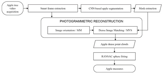
Figure 1.
The Apple3D tool framework.
- Data acquisition: using a smartphone (Figure 2a), a video of an apple tree is recorded, trying to capture apples from multiple positions and angles. Some permanent targets should be located over the plant in order to calibrate the phone’s camera and scale the produced photogrammetric results.
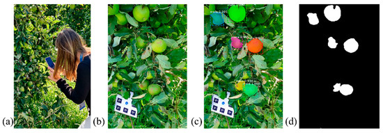 Figure 2. The first part of our framework: video acquisition (a), frame extraction (b), apple detection with an AI method (c) and image mask generation (d).
 - Frame extraction: keyframes are extracted from the acquired video on the smartphone in order to process them using a photogrammetric method. Numerous methods exist in the literature for extracting keyframes. Starting with the performance analysis presented in Torresani and Remodino [40], our tool employs a 2D feature-based approach that discards blurred and redundant frames unsuitable for the photogrammetric process.
- Apple segmentation: a pre-trained neural network model is used for an apple’s instance segmentation on keyframes (Figure 2c). The AI-based method is described in Section 3.2.2 and compared with a clustering approach (Section 3.2.1).
- Mask extraction: the instance segmentation results are converted into binary masks (Figure 2d) in order to isolate fruits and facilitate a dense point cloud generation within the photogrammetric process.
- Image orientation: the extracted keyframes are used for photogrammetric reconstruction purposes, starting from camera pose estimation and sparse point cloud generation (Figure 3a).
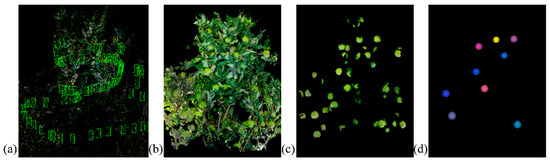 Figure 3. The second part of our framework: image orientation (a), dense point cloud generated without masking the keyframes (b), dense point cloud generated applying masks (c) and fitting spheres on apple instances to derive fruit sizes (d).
 - Dense image matching: using the previously created masks within an MVS (Multi-View Stereo) process, the 3D geometry of the apples is derived (Figure 3b,c). The masking allows for removal of all unwanted areas and partly visible apples. The resulting point clouds are the main product where all measurement experiments are performed.
- Apple size measurement: fitting spheres to the photogrammetric point cloud, sizes and number of fruits are derived (Figure 3d). Two different measuring approaches are presented in Section 3.3.
As the aim of the work is not to introduce a new photogrammetric algorithm but rather to assemble an integrated surveying technique coupled with neural networks in the agriculture field for measuring apple sizes, the reader can find more details about the above-mentioned photogrammetric steps (#2, #5, #6) in the literature [40,41,42,43].
3.2. Apple Segmentation
The ultimate goal of the proposed pipeline is to accurately measure apple sizes using photogrammetrically derived point clouds. In order to optimise these measurements, it is desirable to minimise all possible noise around the fruits. Associating masks to frames to block out all but the single apples during the dense image matching process is an appropriate way to accomplish this.
Two different techniques are tested to automate the apple masking process: a clustering (Section 3.2.1) and a neural-network-based (Section 3.2.2) approach.
3.2.1. Clustering Approach (K-Means)
K-Means Clustering [44] is an unsupervised learning algorithm used for segmenting an unlabelled dataset into K groups of data points (called clusters) based on their similarities. In image segmentation, colour similarities are the most important features. However, due to the high variance in lighting conditions and changes in fruit attributes such as colour and texture, apple segmentation is challenging for in-field acquired images where light and illumination conditions are variable.
Typically, the colour information of images or three-dimensional data are represented using the RGB space. Such a colour space is not suitable for colour-based segmentation processes because spatial proximity, which corresponds to the geometric distance between colour-values, is not coherent with perceptual similarity among colours [45].
Based on these considerations, we converted the video RGB keyframes to CIE L*a*b* colour space [46] before running the unsupervised clustering. In this colour space, one channel is for Luminance (L), and the other two (a* and b*) are known as chromaticity layers. The a* layer indicates where the colour falls along the red-green axis, while the b* layer indicates where it is on the blue-yellow axis. Furthermore, depending on whether the apples were yellow or red, channels a* and b* were used (Figure 4b). For the considered scenario, with a K = 3, frames were automatically segmented into three clusters that could be associated with the “apples”, “leaves”, and “context” classes (Figure 4d). Some morphological operations (erosion and dilation) were then applied to hold only the “apples” class and exclude small items (peduncle, twigs, leaves, etc.) (Figure 4d,e). In particular: (i) all the white segments smaller than 5000 pixels in size were removed and (ii) after finding contours, the contours corresponding to small black holes surrounded by white regions were filled in.
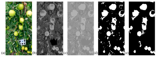
Figure 4.
Clustering approach pipeline: the RGB (a) and L*a*b* (b) keyframes, clustering result (c), masking output (d) and masking output after post-processing (e).
3.2.2. Neural-Network-Based Approach (Mask R-CNN)
Object detection is a computer vision task that involves both the location of one or more objects within an image and the classification of each of these objects [47]. Once located, a bounding box is drawn around each item in the image. An extension of object detection involves marking the specific pixels in the image that belong to each detected object instead of using coarse bounding boxes during object localisation. This harder version of the problem is generally referred to as object segmentation or instance segmentation.
In recent years, deep learning techniques have achieved state-of-the-art results for object detection and semantic segmentation [48,49]. Among the most notable algorithms, we identified the Mask R-CNN [50] as the most suitable for our purposes, as it generates not only a bounding box around the objects but also a pixel-based mask (Figure 5). In our framework, we use the Mask R-CNN model provided by Matterport_Mask_RCNN [51] because it has already been pre-trained on the large-scale object detection, segmentation, and captioning dataset “COCO” [52]. Among the 80 classes included in COCO, there is a specific class for apples, but tests showed that the network was not sufficiently accurate for our scope (see Section 4.3). Starting from the pre-trained weights, a total of about 700 apple instances were manually labelled (using the VIA annotation tool [43]) and used for additional training in order to increase the neural network’s performance.
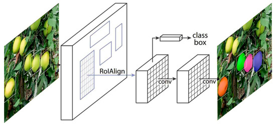
Figure 5.
The Mask R-CNN framework for instance segmentation (adapted from He et al. [50]).
3.3. Apple Size Measuring
In this section, two different methods for measuring the maximum cross-section diameter of the apples are presented: Least Square Fitting (Section 3.3.1) and Random Sample Consensus (RANSAC) (Section 3.3.2).
Both methods are based on the concept of fitting a geometric primitive, i.e., a sphere, to the apples. Figure 6 shows that, independently of apple type and shape, fitting a circle to an apple in an image allows for the extraction of the maximum cross-section diameter. Hence, this principle was extended to the third dimension by fitting spheres to 3D point clouds.
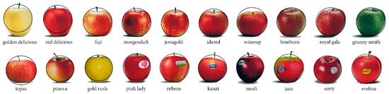
Figure 6.
The overlay of circles to different types of apples shows that a fitting process is suitable to derive the cross-section diameter of the fruit.
3.3.1. Least Square Fitting
The Least Square Fitting method [43] is a statistical approach that finds the best fit of a primitive (e.g., a line, a sphere, etc.) for a set of data (e.g., points) by minimising the sum of the offsets (or residuals) of the data from the fitted primitive.
One of the main advantages of the Least Square Fitting is that it does not require any parameter tuning. On the other hand, it has to work on the single apple instances, though there could be groups of apples that are not always easy to separate. Errors in the instance segmentation would negatively affect the fitting.
3.3.2. RANSAC
The RANdom SAmple Consensus (RANSAC) algorithm [53] is a general parameter estimation approach designed to cope with a large proportion of outliers in the input data. The RANSAC method is used to extract shapes by randomly drawing minimal data points to construct candidate shape primitives. Then, the candidate shapes are checked against all points in the dataset to determine a value for the number of points representing the best fit [54]. Unlike the Least Square Fitting approach, the RANSAC algorithm requires the setting of three parameters:
- (a)
- maximum distance to primitive
- (b)
- sampling resolution
- (c)
- minimum support points per primitive
Considering the desired degree of accuracy, (a) and (b) are set at 3 mm and 6 mm, respectively. In addition, (c) is empirically calculated as follows:
To estimate the number of points per apple, the camera poses derived in the image orientation step are used to reproject every 3D point over the masked images. Then, for each image, the number of points that fall in each apple instance is counted. A median of these values is then computed for the entire dataset of images to estimate the number of points per apple.
4. Experimental Results
In order to assess the proposed pipeline, three types of datasets and scenarios are used:
- synthetic (Section 4.1);
- laboratory (Section 4.2);
- on-field (Section 4.3).
The synthetic datasets are used to evaluate the performance and reliability of the fitting methods, whereas the laboratory and on-field datasets are used to test the effectiveness and accuracy of the entire pipeline.
4.1. Synthetic Datasets
Several experiments were carried out to assess the reliability of the fitting approach for estimating the maximum cross-section diameter. To do this, a set of synthetic apples of various sizes and shapes was built; different 3D models were generated using the open-source software Blender [55], then the meshes were converted into point clouds (i.e., the same outcome of the proposed pipeline). For the sake of completeness, the response of both LSF and RANSAC was tested through various forms of apples (Section 4.1.1), different levels of completeness (Section 4.1.2) and diverse levels of noise in the 3D apples (Section 4.1.3).
4.1.1. Shape (LSF vs. RANSAC)
Starting with four different shapes of apples (Figure 7A–D), the fitting process was evaluated by comparing the radius of the spheres fitted on the point cloud by the LSF and RANSAC algorithms and the actual measurement of the apples (ground truth—GT). According to the results, both RANSAC and LSF established good estimates for apples A, B, and D, while for apple C the RANSAC measurement was more precise than the LSF, whose error was above the 5 mm threshold given by the EU Commission.
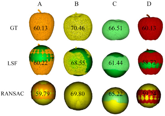
Figure 7.
Measurement comparison between Least Squares Fitting (LSF) and RANSAC approach for different types of apples (A–D) with respect to ground truth (GT) shapes. Measurements are given in millimetres.
4.1.2. Level of Completeness (LSF vs. RANSAC)
The ability of LSF and RANSAC to give accurate measurements with reduced portions of the fruit was tested on the synthetic apples. Each apple was measured either as a whole or cut in 3/4, 1/2 and 1/4.
Table 1 summarises the study results. Unlike the LSF algorithm, the RANSAC algorithm continues to perform even if the fruit completeness decreases. The measuring inaccuracy is less than one mm, even when only a quarter of an apple is utilised.

Table 1.
Measurement (mm) comparison between LSF and RANSAC approach for different synthetic apples (Figure 7) as the completeness of fruits decreases.
4.1.3. Occlusions and Noise (RANSAC)
Synthetic data are further elaborated to recreate datasets as close to reality as possible, including occlusions (Figure 8b) and noise (Figure 8c) in the point clouds. Contrary to the previous experiments where the apples were treated separately, in this case, only the RANSAC algorithm was tested over the fruit composition (Figure 8a). Indeed, such a configuration is not suitable for the LSF method, which works only on single fruits. As shown in Figure 8d, RANSAC was able to fit a geometric primitive (sphere) to each apple. Table 2 reports the diameters of the fitted spheres, with comparisons with ground truth (GT) values. Of the six apples, the one with the most significant measurement error is number five, which deviates by 1.46 mm from the ground truth. Due to the position of the fruit and the presence of occlusions, this inaccuracy is still well below the acceptable threshold given by the EU Commission (5 mm). In addition, the root mean square error (RMSE) with respect to the calliper measurements was calculated, and its value was around 0.84 mm.
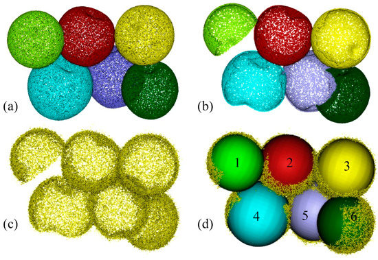
Figure 8.
Generation of a synthetic dataset and testing of the fitting approach: group of synthetic apples (a), introduction of occlusions and not-completeness (b), generation of noise in the point cloud (c), RANSAC fitting results (d).
Table 2.
Fitting results (RANSAC) for each apple of the synthetic dataset (Figure 8). Measurements in mm. RMSE = 0.84 mm.
4.2. Laboratory Tests
An apple tree was built in our laboratory (Figure 9a,b) in order to perform experiments in a controlled environment similar to a real scenario. Before placing the eight apples on the mock plant, each fruit was measured in two ways:
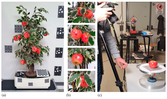
Figure 9.
The built apple tree with eight distributed fruits, check boards and markers for scaling and quality control (a,b). An apple being surveyed on a turntable in the lab (c).
- with a Vernier callipers, taking the average of four measurements for each apple;
- with an accurate photogrammetric survey, placing the apples on a turntable (Ground Sample Distance—GSD—on the apple of approx. 0.1 mm) (Figure 9c), deriving a dense cloud for each apple (Figure 10a,b) and sectioning the cloud to measure the largest diameter (Figure 10c).
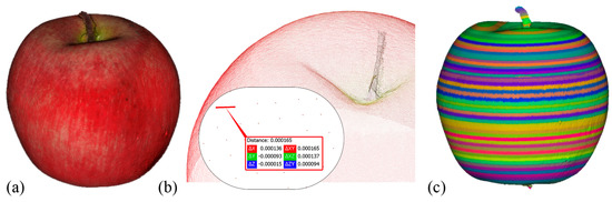 Figure 10. Photogrammetric dense reconstruction of an apple fruit (a), the highlighted point density of the 3D fruit (ca 0.16 mm) (b) and the apple sliced to find the maximum cross-section diameter (c).
Once apples were placed on the tree, the entire pipeline was tested. First, using a Samsung S10 smartphone, a 50 s HD video was captured, and approximately 120 keyframes were extracted. Masks were then generated with both a K-means and mask R-CNN approach. Results showed a decisive improvement in mask R-CNN results after integrating new labelled images into the training (Figure 11).
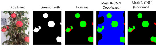
Figure 11.
Comparison of masking performances between K-means and mask R-CNN (True Positive in green, False Negative in red) for the lab images. The re-trained mask R-CNN method delivers better results.
After the image orientation, masks were included in a MVS photogrammetric algorithm to extract the individual 3D fruits (Figure 12). Then, on the generated point clouds of the fruits, both the LSF (after separating the single apples) and RANSAC algorithms were tested to extract the apple measurements. Results (Table 3) show that RANSAC was able to estimate more accurate sizes (except for number three, where both methods failed as the large occlusion prevented a correct fitting).
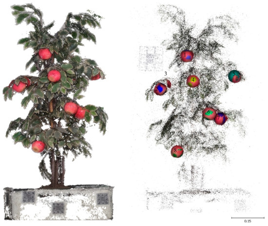
Figure 12.
Photogrammetric reconstruction of the apple tree without (left) and with (right) masking the keyframes. Spheres were then fitted using a RANSAC algorithm.
Table 3.
Measurements (mm) for each apple of the lab tree. RMSEs are calculated with respect to the calliper measurements.
4.3. On-Field Tests
Finally, experiments were carried out in the field. First, coded targets were placed in a stable manner on the trees to (i) scale the photogrammetric projects after the survey and (ii) facilitate the phone’s camera calibration (Figure 13).
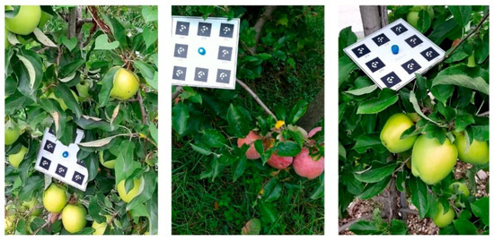
Figure 13.
Examples of targets placed on the apple trees in the field.
For the lab experiment, videos were then recorded and keyframes extracted. Since fruit colours and lighting conditions fluctuate substantially between situations, the two distinct masking procedures were compared. In particular, in order to identify the best approach, for a set of 30 frames, the masking outputs were compared with the manually annotated masks, and the following accuracy metrics were calculated:
where = True positive, = False positive and = False negative.
Precision gives information about a classifier’s performance with respect to false positives (how many apples are found), while Recall provides information about its performance with respect to false negatives (how many apples are missed). If the goal is to minimise False Negatives, then Recall should be as near to 100% as possible without significantly reducing the Precision, whereas if we prefer to minimise False Positives, then Precision should be as close to 100% as possible.
In contrast to the laboratory experiment, the K-means algorithm struggled to distinguish between foliage and apples when data were collected in the field, especially in the case of green apples (Figure 14). Results showed that the re-trained Mask R-CNN outperformed the COCO-based network.
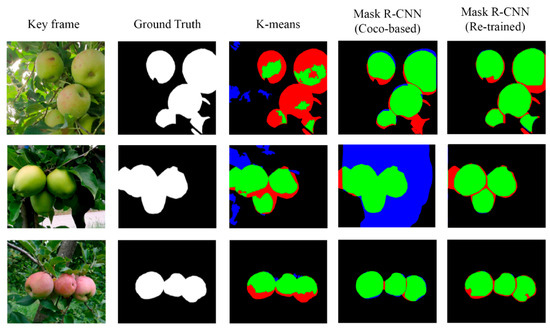
Figure 14.
Comparison of masking performances between K-means and Mask R-CNN approach (True Positive in green, False Negative in red, False Positive in blue) in image sequences acquired in the field. Improvements of the re-trained Mask R-CNN are visible.
The accuracy metrics reported in Table 4 show two differing situations. On the one hand, the K-means with high Recall but low Precision returns many apples, but most of its predictions are inaccurate compared to the ground truth labels. On the other, the re-trained Mask R-CNN with high Precision but low Recall returns fewer apples, but the majority of its predictions are correct.
Table 4.
Accuracy metrics achieved for the masking process using K-means and Mask R-CNN approaches.
Given that the same apple to be reconstructed in the photogrammetric process would appear in multiple frames, the fact that an algorithm occasionally misses some fruits is not a major issue because the likelihood that it will occur in nearby frames is very high. It is critical that the reconstructed point cloud only includes fruits and not foliage, as this could affect the accuracy of the fitting measurement. Given these factors, it was determined that the mask R-CNN was the optimum method for the case study.
Once the extracted and masked frames were processed, we could compare the on-field measurements (acquired by callipers) with the ones extracted by fitting the spheres to the 3D point clouds (Figure 15). Even in the field, errors persist in the order of a few millimetres, i.e., within the expected errors given by the EU regulations.
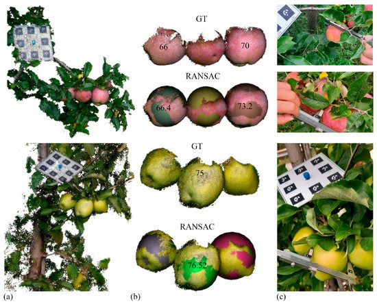
Figure 15.
Experimental results with real data in the field: dense photogrammetric point cloud (only for display purposes) (a), fitting results and measurements comparison with the point cloud derived from the masked images (b) and on-field measurements using a Vernier callipers (c).
5. Discussion and Conclusions
The paper presented a new framework to measure apple sizes from smartphone-based videos, exploiting photogrammetric and artificial intelligence methods. Different types of tests were performed to validate the methodology, with both synthetic and real data in the lab and in the field.
In the image masking phase, the comparison between K-means and Mask R-CNN showed that under ideal lighting conditions and with red apples, the two systems are almost equivalent. However, field tests shows that the R-CNN approach is more reliable in terms of light and fruit colour changes. Moreover, the results displayed that the re-trained network outperformed the COCO-based network. Nguyen et al. [21], in their study, reported 100% precision in detecting fully visible apples and 82% for partially occluded apples. In our case, 85% of occluded apples were detected and correctly masked.
In terms of measurement approaches, LSF proved to be inadequate when fruit portions were small (e.g., occluded by leaves). On the other hand, RANSAC allowed correct measurements to be extrapolated in the presence of various varieties of apples, both for occlusions and completeness. For the synthetic dataset, the RMSE was below 1 mm while for the laboratory dataset it was around 4 mm. These results are in line with or even better than those specified in the literature: Stajnko et al. [18] reported a RMSE of 7 mm, whereas Regunanthan et al. [20] achieved 4 mm. Wang et al. [22] achieved similar results, measuring mango fruits with a RMSE of 4.9 mm along the length and 4.3 mm across the width.
The achieved results show how the use of new technologies could provide support to farmers. The strengths of the presented framework are:
- The achievement of precise measurements using 3D point clouds.
- The use of low-cost and common instruments (smartphones) for fruit surveying.
- The introduction of a less subjective approach for measuring fruits compared to callipers, providing at the same time a more extensive set of apples measured in the field (Figure 16).
 Figure 16. Experiments in the field: a keyframe extracted from a short smartphone video (37 sec) (a), the photogrammetric dense point cloud with (b) and without (c) masking the images, and the output from the RANSAC fitting, which allows quantification of the number of fruits on the tree (d).
 - The availability of videos for experiments, masking code, labelled images for re-training, and network weights at 3DOM-FBK-GitHub [56].
The weaknesses of the presented framework are as follows:
- The sensitivity to illumination variations and changes in the apple shapes: when the video is captured around midday or in cloudy conditions, the lighting issues are minimised.
- The need of placing a target in the field to derive metric results from the photogrammetric processing: the authors are planning new acquisitions with an in-house developed stereo-vision system [57], which does not require in-field targets to scale the results.
- The reliability in masking green apples, as their colour is very similar to the leaves: the authors are planning to refine the masking method, enriching the neural network with more training images.
As future research lines, the following aspects may deserve attention and further development:
- Verifying the application of the method to similar fruits (i.e., pears, kiwi, etc.).
- Using colour information, available in the videos, to support analyses related to fruit maturation.
- Adapting the proposed framework to on-field quality control, inspection and detection of damage over the fruit surface due, for example, to bad meteorological conditions.
- Finalization of the deployment of the entire framework in Cloud so users can acquire videos with a smartphone in the field and access Cloud resources to derive measurements almost in real time.
Author Contributions
Conceptualization, E.G. and F.R.; methodology, E.G.; software, R.B.; validation, E.G.; formal analysis, E.G.; investigation, E.G.; resources, F.R.; data curation, E.G. and R.B.; writing—original draft preparation, E.G.; writing—review and editing, F.R.; visualization, E.G.; supervision, F.R. All authors have read and agreed to the published version of the manuscript.
Funding
This research received no external funding.
Data Availability Statement
Data acquired and used in the presented experiments, labelled images, code, and network weights, are available to the scientific community at 3DOM-FBK-GitHub [56].
Conflicts of Interest
The authors declare no conflict of interest.
References
- European Commision Website. Available online: https://ec.europa.eu/info/food-farming-fisheries/plants-and-plant-products/fruits-and-vegetables_en (accessed on 1 September 2021).
- Jideani, A.I.; Anyasi, T.; Mchau, G.R.; Udoro, E.O.; Onipe, O.O. Processing and preservation of fresh-cut fruit and vegetable products. Postharvest Handling 2017, 47–73. [Google Scholar] [CrossRef] [Green Version]
- 543/2011/EU: Commission Implementing Regulation (EU) No 543/2011 of 7 June 2011 Laying Down Detailed Rules for the Application of Council Regulation (EC) No 1234/2007 in Respect of the Fruit and Vegetables and Processed Fruit and Vegetables Sectors; European Union: Luxembourg, 2011.
- Marini, R.P.; Schupp, J.R.; Baugher, T.A.; Crassweller, R. Estimating apple fruit size distribution from early-season fruit diameter measurements. HortScience 2019, 54, 1947–1954. [Google Scholar] [CrossRef] [Green Version]
- Navarro, E.; Costa, N.; Pereira, A. A systematic review of iot solutions for smart farming. Sensors 2020, 20, 4231. [Google Scholar] [CrossRef] [PubMed]
- Yousefi, M.R.; Razadari, A.M. Application of GIS and GPS in precision agriculture (A review). Int. J. Adv. Biol Biom Res. 2015, 3, 7–9. [Google Scholar]
- Pivoto, D.; Waquil, P.D.; Talamini, E.; Finocchio, C.P.S.; Dalla Corte, V.F.; de Vargas Mores, G. Scientific development of smart farming technologies and their application in Brazil. Inf. Process. Agric. 2018, 5, 21–32. [Google Scholar] [CrossRef]
- De Mauro, A.; Greco, M.; Grimaldi, M. A formal definition of Big Data based on its essential features. Libr. Rev. 2016, 65, 122–135. [Google Scholar] [CrossRef]
- Daponte, P.; De Vito, L.; Glielmo, L.; Iannelli, L.; Liuzza, D.; Picariello, F.; Silano, G. A Review on the Use of Drones for Precision Agriculture; IOP Publishing: Bristol, UK, 2019; Volume 275, p. 012022. [Google Scholar]
- Tsolakis, N.; Bechtsis, D.; Bochtis, D. AgROS: A robot operating system based emulation tool for agricultural robotics. Agronomy 2019, 9, 403. [Google Scholar] [CrossRef] [Green Version]
- Talaviya, T.; Shah, D.; Patel, N.; Yagnik, H.; Shah, M. Implementation of artificial intelligence in agriculture for optimisation of irrigation and application of pesticides and herbicides. Artif. Intell. Agric. 2020, 4, 58–73. [Google Scholar] [CrossRef]
- Linaza, M.; Posada, J.; Bund, J.; Eisert, P.; Quartulli, M.; Döllner, J.; Pagani, A.; Olaizola, I.G.; Barriguinha, A.; Moysiadis, T.; et al. Data-driven artificial intelligence applications for sustainable precision agriculture. Agronomy 2021, 11, 1227. [Google Scholar] [CrossRef]
- Blanpied, G.; Silsby, K. Predicting Harvest Date Windows for Apples; Cornell Coop. Extension: New York, NY, USA, 1992. [Google Scholar]
- Moreda, G.; Ortiz-Cañavate, J.; Ramos, F.J.G.; Altisent, M.R. Non-destructive technologies for fruit and vegetable size determination—A review. J. Food Eng. 2009, 92, 119–136. [Google Scholar] [CrossRef] [Green Version]
- Zujevs, A.; Osadcuks, V.; Ahrendt, P. Trends in robotic sensor technologies for fruit harvesting: 2010–2015. Procedia Comput. Sci. 2015, 77, 227–233. [Google Scholar] [CrossRef]
- Song, J.; Fan, L.; Forney, C.F.; Mcrae, K.; Jordan, M.A. The relationship between chlorophyll fluorescence and fruit quality indices in “jonagold” and “gloster” apples during ripening. In Proceedings of the 5th International Postharvest Symposium 2005, Verona, Italy, 6–11 June 2004; Volume 682, pp. 1371–1377. [Google Scholar]
- Das, A.J.; Wahi, A.; Kothari, I.; Raskar, R. Ultra-portable, wireless smartphone spectrometer for rapid, non-destructive testing of fruit ripeness. Sci. Rep. 2016, 6, srep32504. [Google Scholar] [CrossRef] [Green Version]
- Stajnko, D.; Lakota, M.; Hočevar, M. Estimation of number and diameter of apple fruits in an orchard during the growing season by thermal imaging. Comput. Electron. Agric. 2004, 42, 31–42. [Google Scholar] [CrossRef]
- Payne, A.; Walsh, K.; Subedi, P.; Jarvis, D. Estimating mango crop yield using image analysis using fruit at ‘stone hardening’ stage and night time imaging. Comput. Electron. Agric. 2014, 100, 160–167. [Google Scholar] [CrossRef]
- Regunathan, M.; Lee, W.S. Citrus fruit identification and size determination using machine vision and ultrasonic sensors. In Proceedings of the 2005 ASAE Annual Meeting, American Society of Agricultural and Biological Engineers, Tampa, FL, USA, 17–20 July 2005. [Google Scholar]
- Nguyen, T.T.; Vandevoorde, K.; Wouters, N.; Kayacan, E.; De Baerdemaeker, J.G.; Saeys, W. Detection of red and bicoloured apples on tree with an RGB-D camera. Biosyst. Eng. 2016, 146, 33–44. [Google Scholar] [CrossRef]
- Wang, Z.; Walsh, K.B.; Verma, B. On-tree mango fruit size estimation using RGB-D images. Sensors 2017, 17, 2738. [Google Scholar] [CrossRef] [PubMed] [Green Version]
- Font, D.; Pallejà, T.; Tresanchez, M.; Runcan, D.; Moreno, J.; Martínez, D.; Teixidó, M.; Palacín, J. A proposal for automatic fruit harvesting by combining a low cost stereovision camera and a robotic arm. Sensors 2014, 14, 11557–11579. [Google Scholar] [CrossRef] [Green Version]
- Gongal, A.; Karkee, M.; Amatya, S. Apple fruit size estimation using a 3D machine vision system. Inf. Process. Agric. 2018, 5, 498–503. [Google Scholar] [CrossRef]
- Cubero, S.; Aleixos, N.; Moltó, E.; Gómez-Sanchis, J.; Blasco, J. Advances in machine vision applications for automatic inspection and quality evaluation of fruits and vegetables. Food Bioprocess Technol. 2011, 4, 487–504. [Google Scholar] [CrossRef]
- Saldaña, E.; Siche, R.; Luján, M.; Quevedo, R. Review: Computer vision applied to the inspection and quality control of fruits and vegetables. Braz. J. Food Technol. 2013, 16, 254–272. [Google Scholar] [CrossRef] [Green Version]
- Naik, S.; Patel, B. Machine Vision based Fruit Classification and Grading—A Review. Int. J. Comput. Appl. 2017, 170, 22–34. [Google Scholar] [CrossRef]
- Hung, C.; Nieto, J.; Taylor, Z.; Underwood, J.; Sukkarieh, S. Orchard fruit segmentation using multi-spectral feature learning. In Proceedings of the 2013 IEEE/RSJ International Conference on Intelligent Robots and Systems, Tokyo, Japan, 3–7 November 2013; pp. 5314–5320. [Google Scholar]
- Sa, I.; Ge, Z.; Dayoub, F.; Upcroft, B.; Perez, T.; McCool, C. DeepFruits: A fruit detection system using deep neural networks. Sensors 2016, 16, 1222. [Google Scholar] [CrossRef] [Green Version]
- Cheng, H.; Damerow, L.; Sun, Y.; Blanke, M. Early yield prediction using image analysis of apple fruit and tree canopy features with neural networks. J. Imaging 2017, 3, 6. [Google Scholar] [CrossRef]
- Hambali, H.A.; Sls, A.; Jamil, N.; Harun, H. Fruit classification using neural network model. J. Telecommun. Electron. Comput Eng. 2017, 9, 43–46. [Google Scholar]
- Hossain, M.S.; Al-Hammadi, M.H.; Muhammad, G. Automatic fruit classification using deep learning for industrial applications. IEEE Trans. Ind. Inform. 2019, 15, 1027–1034. [Google Scholar] [CrossRef]
- Siddiqi, R. Comparative performance of various deep learning based models in fruit image classification. In Proceedings of the 11th International Conference on Advances in Information Technology, Bangkok, Thailand, 1–3 July 2020; Association for Computing Machinery (ACM): New York, NY, USA, 2020; pp. 1–9. [Google Scholar]
- Mureşan, H.; Oltean, M. Fruit recognition from images using deep learning. Acta Univ. Sapientiae Inform. 2018, 10, 26–42. [Google Scholar] [CrossRef] [Green Version]
- Gongal, A.; Amatya, S.; Karkee, M.; Zhang, Q.; Lewis, K. Sensors and systems for fruit detection and localization: A review. Comput. Electron. Agric. 2015, 116, 8–19. [Google Scholar] [CrossRef]
- Tao, Y.; Zhou, J. Automatic apple recognition based on the fusion of color and 3D feature for robotic fruit picking. Comput. Electron. Agric. 2017, 142, 388–396. [Google Scholar] [CrossRef]
- Hua, Y.; Zhang, N.; Yuan, X.; Quan, L.; Yang, J.; Nagasaka, K.; Zhou, X.-G. Recent advances in intelligent automated fruit harvesting robots. Open Agric. J. 2019, 13, 101–106. [Google Scholar] [CrossRef] [Green Version]
- Onishi, Y.; Yoshida, T.; Kurita, H.; Fukao, T.; Arihara, H.; Iwai, A. An automated fruit harvesting robot by using deep learning. Robomech J. 2019, 6, 1–8. [Google Scholar] [CrossRef] [Green Version]
- Tang, Y.; Chen, M.; Wang, C.; Luo, L.; Li, J.; Lian, G.; Zou, X. Recognition and localization methods for vision-based fruit picking robots: A review. Front. Plant Sci. 2020, 11, 510. [Google Scholar] [CrossRef]
- Torresani, A.; Remondino, F. Videogrammetry vs. photogrammetry for heritage 3D reconstruction. ISPRS—Int. Arch. Photogramm. Remote Sens. Spat. Inf. Sci. 2019, XLII-2/W15, 1157–1162. [Google Scholar] [CrossRef] [Green Version]
- Remondino, F.; Spera, M.G.; Nocerino, E.; Menna, F.; Nex, F.C. State of the art in high density image matching. Photogramm. Rec. 2014, 29, 144–166. [Google Scholar] [CrossRef] [Green Version]
- Stathopoulou, E.-K.; Welponer, M.; Remondino, F. Open-source image-based 3D reconstruction pipelines: Review, comparison and evaluation. ISPRS—Int. Arch. Photogramm. Remote Sens. Spat. Inf. Sci. 2019, XLII-2/W17, 331–338. [Google Scholar] [CrossRef] [Green Version]
- Stathopoulou, E.; Battisti, R.; Cernea, D.; Remondino, F.; Georgopoulos, A. Semantically derived geometric constraints for MVS reconstruction of textureless areas. Remote Sens. 2021, 13, 1053. [Google Scholar] [CrossRef]
- Likas, A.; Vlassis, N.; Verbeek, J.J. The global k-means clustering algorithm. Pattern Recognit. 2003, 36, 451–461. [Google Scholar] [CrossRef] [Green Version]
- Bora, D.J.; Gupta, A.K. A New Approach towards clustering based color image segmentation. Int. J. Comput. Appl. 2014, 107, 23–30. [Google Scholar] [CrossRef]
- Robertson, A.R. The CIE 1976 color-difference formulae. Color Res. Appl. 1977, 2, 7–11. [Google Scholar] [CrossRef]
- Dasiopoulou, S.; Mezaris, V.; Kompatsiaris, I.; Papastathis, V.-K.; Strintzis, M. Knowledge-assisted semantic video object detection. IEEE Trans. Circuits Syst. Video Technol. 2005, 15, 1210–1224. [Google Scholar] [CrossRef]
- Minaee, S.; Boykov, Y.Y.; Porikli, F.; Plaza, A.J.; Kehtarnavaz, N.; Terzopoulos, D. Image segmentation using deep learning: A survey. IEEE Trans. Pattern Anal. Mach. Intell. 2021. [Google Scholar] [CrossRef]
- Griffiths, D.; Boehm, J. A review on deep learning techniques for 3D sensed data classification. Remote Sens. 2019, 11, 1499. [Google Scholar] [CrossRef] [Green Version]
- He, K.; Gkioxari, G.; Dollár, P.; Girshick, R.B. Mask R-CNN. IEEE Trans. Pattern Anal. Mach. Intell. 2020, 42, 386–397. [Google Scholar] [CrossRef] [PubMed]
- Abdulla, W. Mask R-CNN for Object Detection and Instance Segmentation on Keras and TensorFlow; GitHub Repository: San Francisco, CA, USA, 2017. [Google Scholar]
- Lin, T.-Y.; Maire, M.; Belongie, S.; Hays, J.; Perona, P.; Ramanan, D.; Dollár, P.; Zitnick, C.L. Microsoft COCO: Common objects in context. In Computer Vision—ECCV 2014; Fleet, D., Pajdla, T., Schiele, B., Tuytelaars, T., Eds.; Springer: Cham, Switzerland, 2014. [Google Scholar] [CrossRef] [Green Version]
- Schnabel, R.; Wahl, R.; Klein, R. Efficient RANSAC for point-cloud shape detection. Comput. Graph. Forum 2007, 26, 214–226. [Google Scholar] [CrossRef]
- Grilli, E.; Menna, F.; Remondino, F. A review of point clouds segmentation and classification algorithms. ISPRS—Int. Arch. Photogramm. Remote Sens. Spat. Inf. Sci. 2017, XLII-2/W3, 339–344. [Google Scholar] [CrossRef] [Green Version]
- Community BO. Blender—A 3D Modelling and Rendering Package; Stichting Blender Foundation: Amsterdam, The Netherlands; Available online: http://www.blender.org (accessed on 1 September 2021).
- 3DOM-FBK-GitHub. Available online: https://github.com/3DOM-FBK/Mask_RCNN/tree/master/samples/apples (accessed on 25 September 2021).
- Torresani, A.; Menna, F.; Battisti, R.; Remondino, F. A V-SLAM guided and portable system for photogrammetric applications. Remote Sens. 2021, 13, 2351. [Google Scholar] [CrossRef]
Publisher’s Note: MDPI stays neutral with regard to jurisdictional claims in published maps and institutional affiliations. |
© 2021 by the authors. Licensee MDPI, Basel, Switzerland. This article is an open access article distributed under the terms and conditions of the Creative Commons Attribution (CC BY) license (https://creativecommons.org/licenses/by/4.0/).