Environmental Sensitivity of Large Stealth Longwave Antenna Systems

Abstract

This article presents an analysis of measurements collected during a six-month-long experimental deployment of a surface-placed horizontal magnetic loop antenna. The changes in the measured parameters of the loop are investigated in relation to the surrounding environment’s composition, temperature and water content. Basic functions describing these changes are formulated. The results are confronted with outcomes from similar experiments from previous years and different locations, showing good compliance. The developed functions and antenna system can be used for environmental monitoring of soil composition and humidity over large areas and volumes, helpful in, for example, flood awareness.

1. Introduction

Longwave (LW, low frequency, 30–300 kHz) and lower frequency operating antenna systems are frequently used for communications with submerged submarines, transmissions of teleswitches, frequency and time standards, and broadcasting and remote sensing of rock layers using various versions of the transmitting equipment [1]. Many of these methods have successfully investigated ground properties using longwave signals emitted by commercial or national radio stations, for example, Felsberg-Berus on 183 kHz [2] (Europe 1, now inactive) or RTCN Raszyn-Łazy on 227 kHz [3] (Polish Radio Program 1, now 225 kHz from Solec Kujawski [4]). However, in many research locations, it is difficult to deploy a dedicated LW transmitting system—either due to its power demands or the physical dimensions of the desired transmitting antenna, which often require elaborated mechanical supportive structures [5]. A solution to this issue is the use of either airborne antenna systems [2,6,7] or stealth ground-located antennas, composed of horizontal loops [8], horizontal dipoles [5,9] or antennas composed of natural terrain structures [10,11,12]. Such radiators are able to operate as elements of a wider system of communication (for example in a mine [13]) or as a standalone system that investigates the properties of the surrounding environment.

This work aims to define the sources of the unstable behaviour of the parameters of stealth longwave horizontal loop antennas; this instability manifests itself in rapid changes in the antenna’s inductance, which can be linked to direct changes in the surrounding environment (despite operation on low and lower frequencies). Similar instabilities have been recorded in the past years by Fenwick and Weeks (1963) [5], Barr and Ireland (1993) [14] and Miś and Modelski (2020) [15], yet there is still no direct explanation of the phenomena. In this work, this phenomena will be explained and described in formulas which will allow for the estimation of the unstable behaviour of given antenna parameters for the next experiments in this field—both as potential sources for antenna detuning and as potential means of wide-range remote sensing of the surrounding ground.

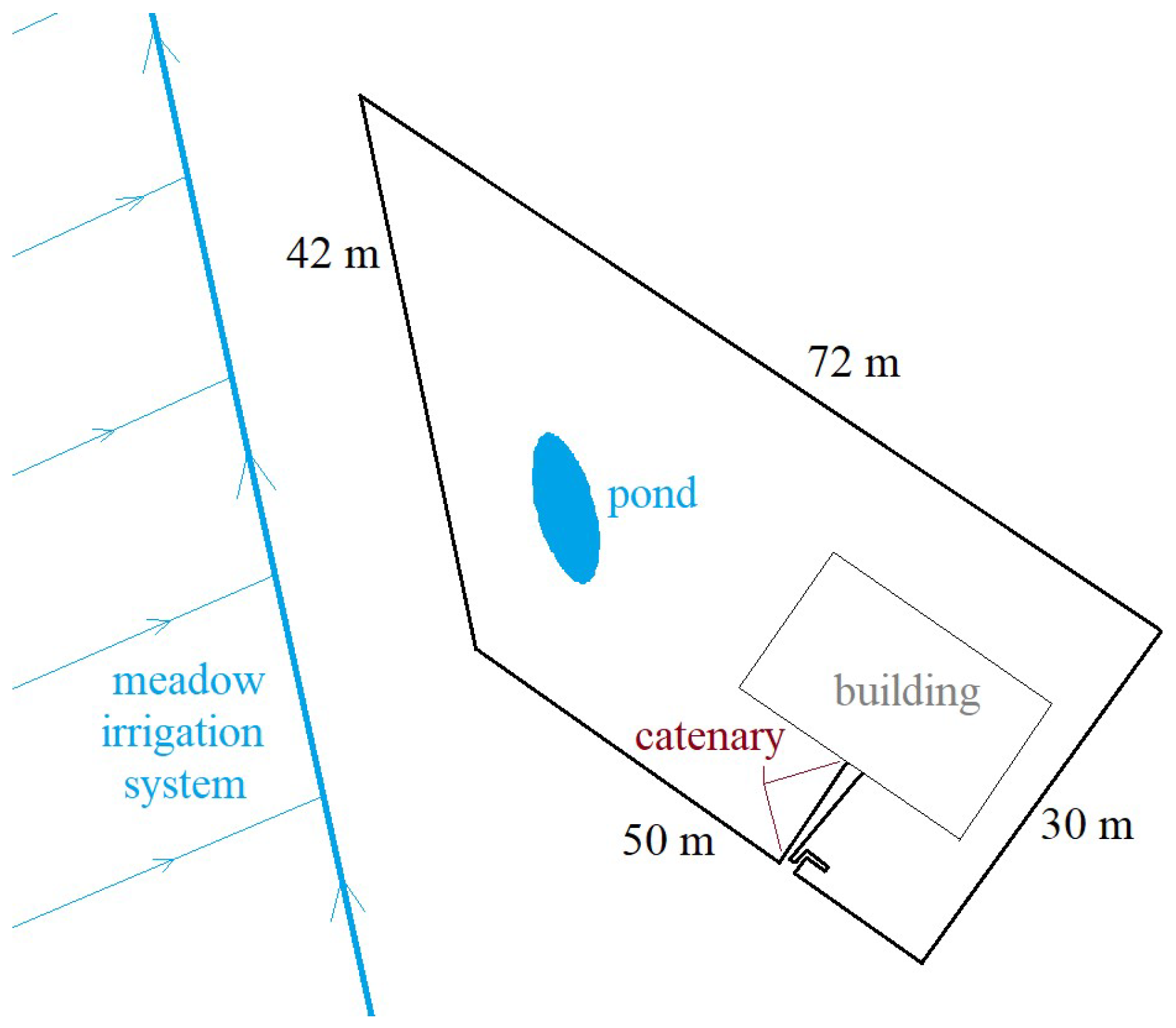
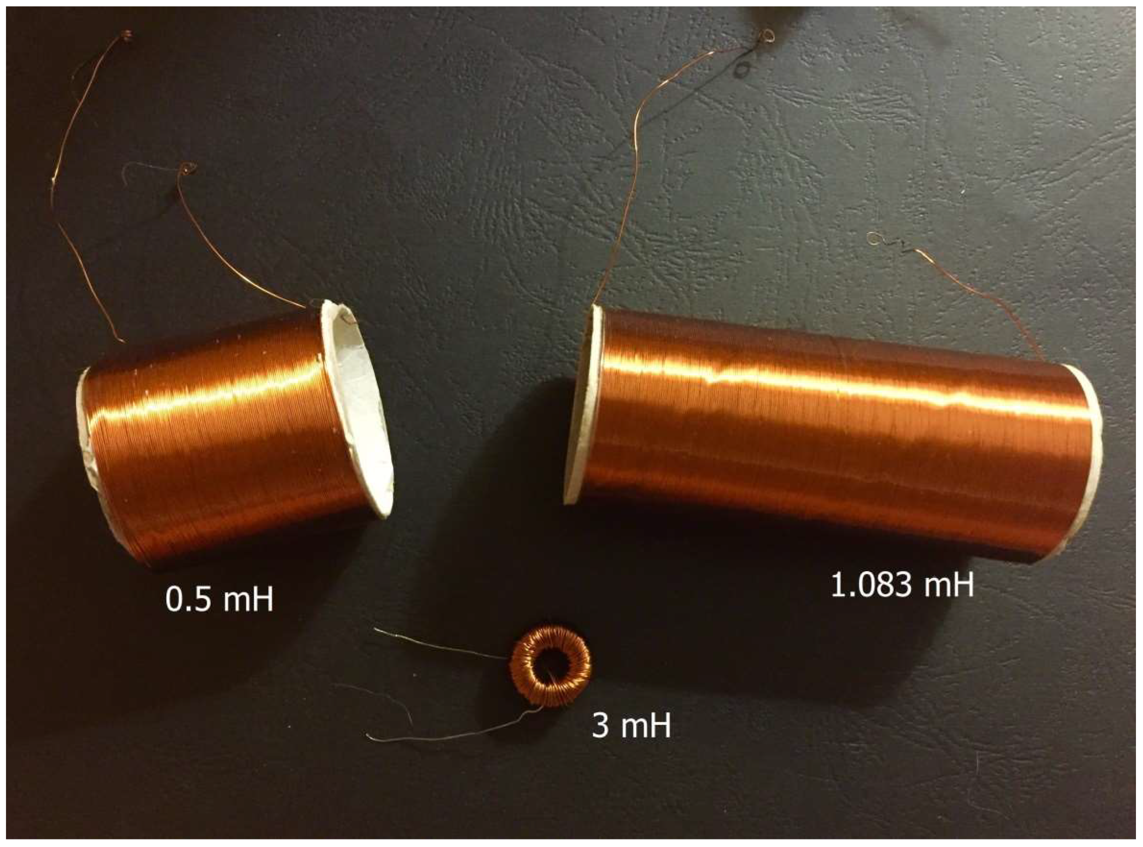
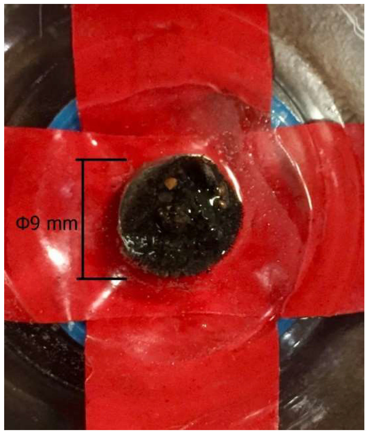
2. Experiment Setup

In order to allow a direct detection and comparison of measured antenna parameters (as well as future research on loop antenna performance using 198 kHz broadcasting frequency [16]), the test antenna system was deployed similarly to the systems used in glacial ice during the 2019 campaign of the IGLUNA: A Habitat in Ice program by Swiss Space Center (an ESA_Lab initiative) [17]. Over a large area south of Warsaw, Poland, a trapezoidal loop antenna was laid directly on the ground, as shown on Figure 1. The copper antenna wire had the cross-section area of 0.35 mm² and was entirely insulated by a PVC layer. As in the IGLUNA 2019 experiments, the total electrical length of the loose cable was 278 m [18,19]. The feed point of the antenna was located close to the building, inside the loop. The feeder setup formed a two-wire catenary approximately 2 m above the surface (see Figure 2). The feeders entered the ground through clay inlets/wells approximately 2 cm below the surface, and emerged less than 1 m away to form the proper loop. The antenna feed points remained constant during the experiments (in contrary to Barr’s and Ireland’s works [14], but in accordance to IGLUNA 2019 [18]); the wire ends were secured in metal banana-type plugs with removable covers.

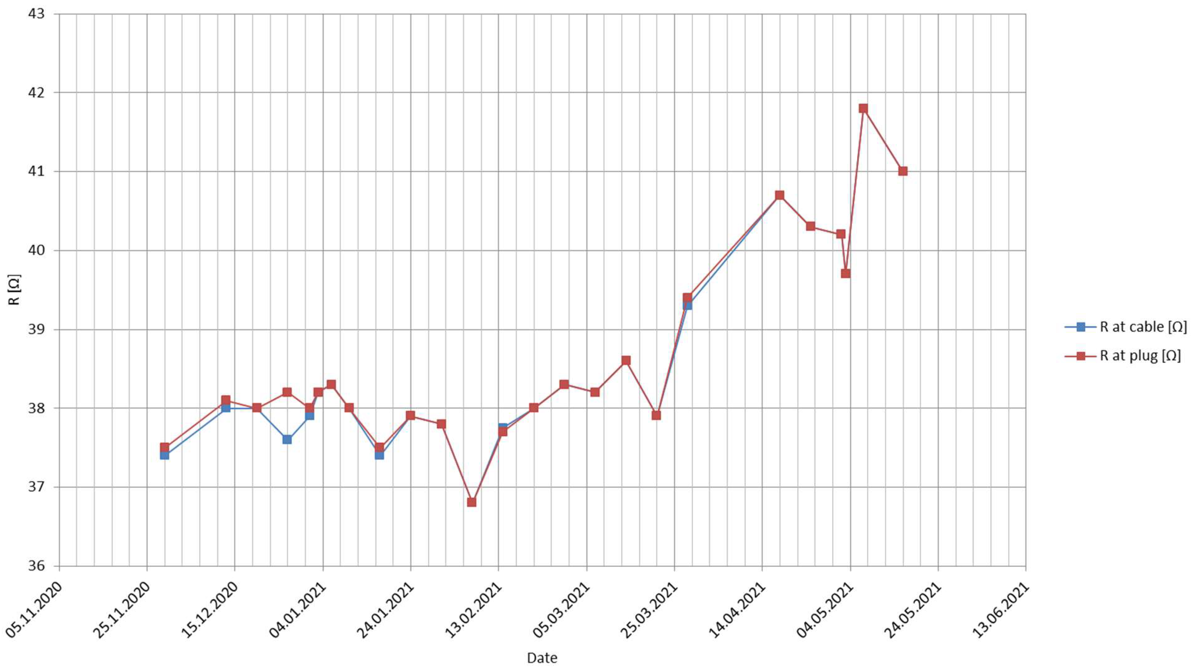
3. Longtime Measurements

The inductance and DC resistance of the deployed antenna were measured between 29 November 2020 and 16 May 2021 on an approximately weekly basis. The measurements were taken using an AXIOMET AX-588B digital meter with an inductance probing frequency of 100 Hz [20].

As predicted, and similarly to the IGLUNA 2019 experiments, the inductance indications varied, in most cases exceeding the ±2.5% toleration of indication of the measuring device [20]—the recorded values are presented on Figure 3 (from each measured inductance value the inductance of the meter’s cables, measured shortly after the antenna, was subtracted). The ranges of the inductance values did not remain constant and changed with the environmental changes, which shall be investigated below.

Figure 4 presents the measurements of the DC resistance of the bare antenna cable (‘R at cable’) and the antenna cable fitted with plugs, with the meter’s probes positioned on the plugs (‘R at plug’). The values generally follow the temperature changes of the environment, as well as the humidity; in one measurement, a significant difference was noted between the cable and the plug, most likely due to the dew presence on the plug, which prevented in later measurements. After 18th April, the antenna was repaired (soldered) in two locations—in the later days, the DC resistance of the wire increased due to the natural rise in the surrounding air temperature.

As the antenna measurements spanned over nearly half a year, the response of the antenna system to the environmental changes—such as changes in the humidity/water content, temperature, and type of precipitation—can be clearly noticed through the winter and spring months. These changes, entailing the variations in the antenna parameters crucial for its stable functioning as an electromagnetic (EM) radiating structure, require an investigation that should lead to the definition of their origin and the development of a mean of their predictions in the given environmental conditions. To reach these goals, hypotheses of the origins of the aforementioned changes were formed and tested.

4. System Parameters’ Simulations

In order to clearly define the physical phenomena responsible for the detected variations in the parameters mentioned in the previous Section, a direct link must be defined between the variability of the environmental conditions and the parameters measured in the longtime campaign. This link must be defined using given constraints:

•

Main relation to the measured primary parameter of the loop (the inductance);

•

Dependence on the temperature and humidity;

•

Detectability by the employed measuring device.

After the formulation, each hypothesis of such links was verified by design or applicable analysis/simulation—if changes related to the surrounding environment were detected in at least one hypothesis, then this hypothesis would be considered as the one explaining the behaviour of the measured parameters; if multiple hypotheses presented such relations, then a deeper analysis of these hypotheses would be performed (not necessarily excluding one of them, and possibly showing a coexistence of multiple sources of the encountered measurements’ behaviour).

The initial hypothesis explaining the changes in the antenna inductance (antenna considered as a magnetic loop) employed thermal contraction and expansion of the antenna cable itself (wire with insulation), which, regarding its length, could appear significant enough to change the inductance of the loop (proportional to the natural logarithm of the loop’s perimeter [14]). However, the thermal expansion coefficients of the cable’s materials were found to be too low to cause a significant (relative to the total electrical length) change in the length of the cable [21]; therefore, its influence on the measured inductance was considered negligible. Subsequent hypotheses were formed based on the direct properties of the environment surrounding the antenna, compatible with the constraints given above:

•

The measured inductance values are directly related to the inductance of the components of the surrounding environment, which may change with temperature and humidity (liquid water causing ferromagnetic particle movements over a large area etc.)—Section 4.1;

•

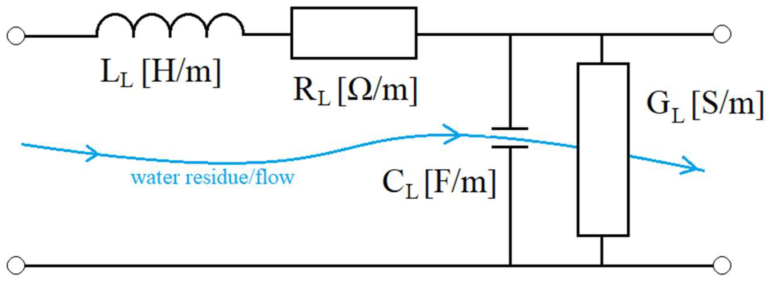
The changing state of the environment (liquid water, snow, ice) may change the linear parameters of the antenna considered as a transmission line, which—given the probing frequency of the measuring device—may show the changes on the measured parameters—Section 4.2;

•

The functioning of the measuring device (the differentiating circuit of the digital meter) may indirectly employ a physical parameter, which is environmentally dependent and, therefore, may influence the measured parameters—Section 4.3.

4.1. Approach for The Environment’s Inductance

As the antenna is located on the surface of the ground, it can be considered as a magnetic loop antenna with a half-buried ground core [14]; water circulation in this core depends on the composition of the soil (defining its ability to accumulate a finite amount of water per mass unit [22]) the precipitation and the formation of subsurface water flow [23] (both on a smaller scale and larger scale, including anthropogenic factors like the irrigation system shown in Figure 1, which not only causes water flow, but also changes the level of the subsurface water layer [24] in proximity to the loop). If a sufficient amount of charged particles is present in the flow—dissociated salts, iron oxide domains—in the presence of a static magnetic field (created by, for example, immobile layers of soil enriched in iron oxides, or the magnetic field of the loop antenna itself during the measurements), an inductance can be defined and measured [25].

To investigate the magnetic properties of the soil, a series of inductors with 0.5, 1.084 and 3 mH (one, two and six times the approximate mean value of the measured inductance; see Figure 5) were measured with cores made of direct soil samples, water samples from the antenna surroundings (including moving water) and pure iron oxides extracted from 200 g of soil sample. In all cases, the inductance values did not vary. The soil profile, depicting its fractional composition, is shown in Figure 6; the amount of iron oxides extracted from it is shown in Figure 7. The mass of extracted iron oxides was calculated as 0.571 g per 200 g of soil sample, which appeared to be too low to cause a distortion of the inductance measurement.

The composition of the soil, showing a large share of illite fraction, suggested a high ability of water absorption; using the method of soil drying [22], the maximum achievable absorbed amount of water was computed as 0.357 kg per 1 kg of dry soil. Therefore, new hypotheses, linked directly to the fact of water accumulation, had to be formed—this action was backed up by the analysis of the magnetic loop antenna measurements from IGLUNA 2019 [15], where the wires were positioned in pure glacial ice, with no iron oxide domains, and the inductance values did not remain constant.

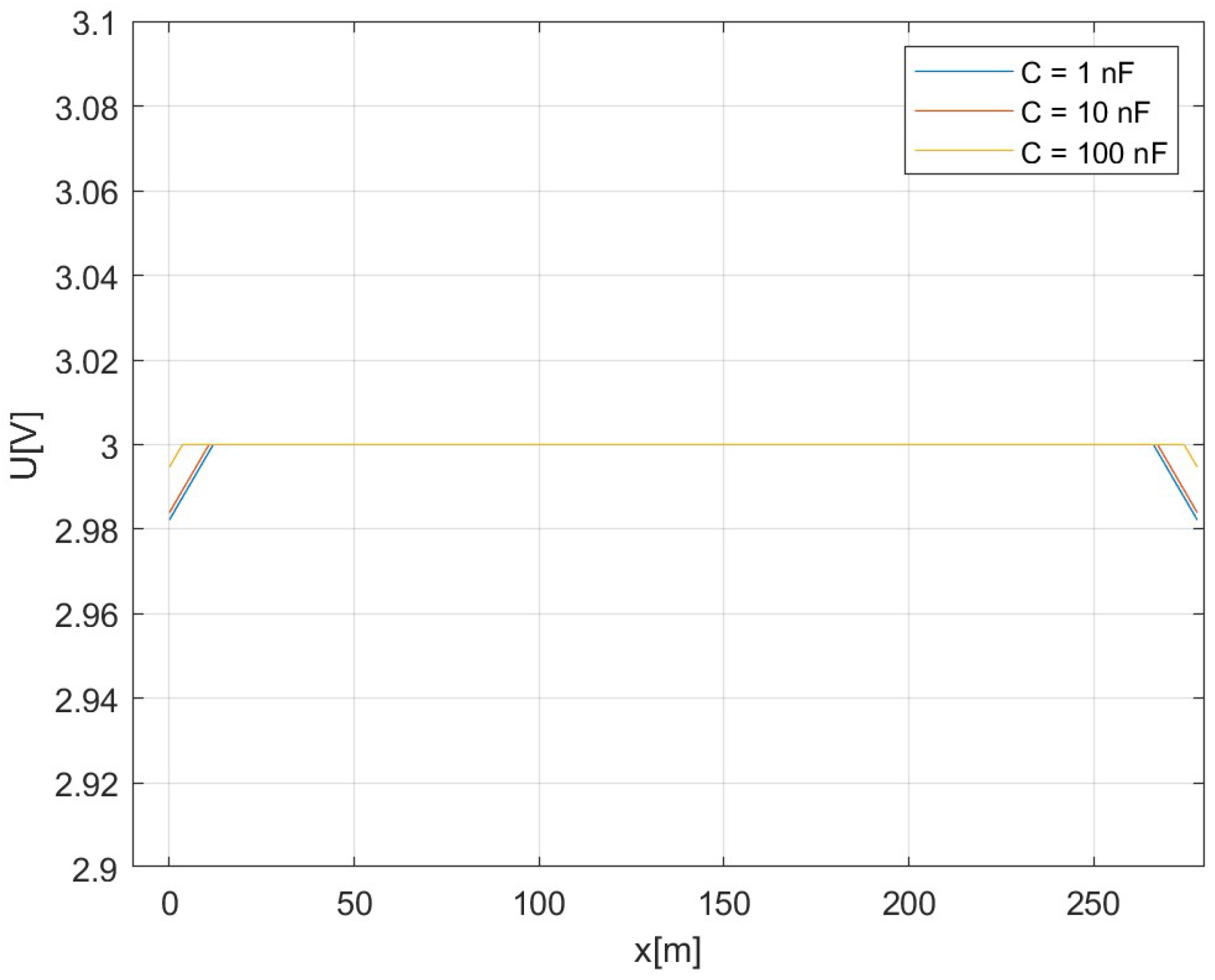
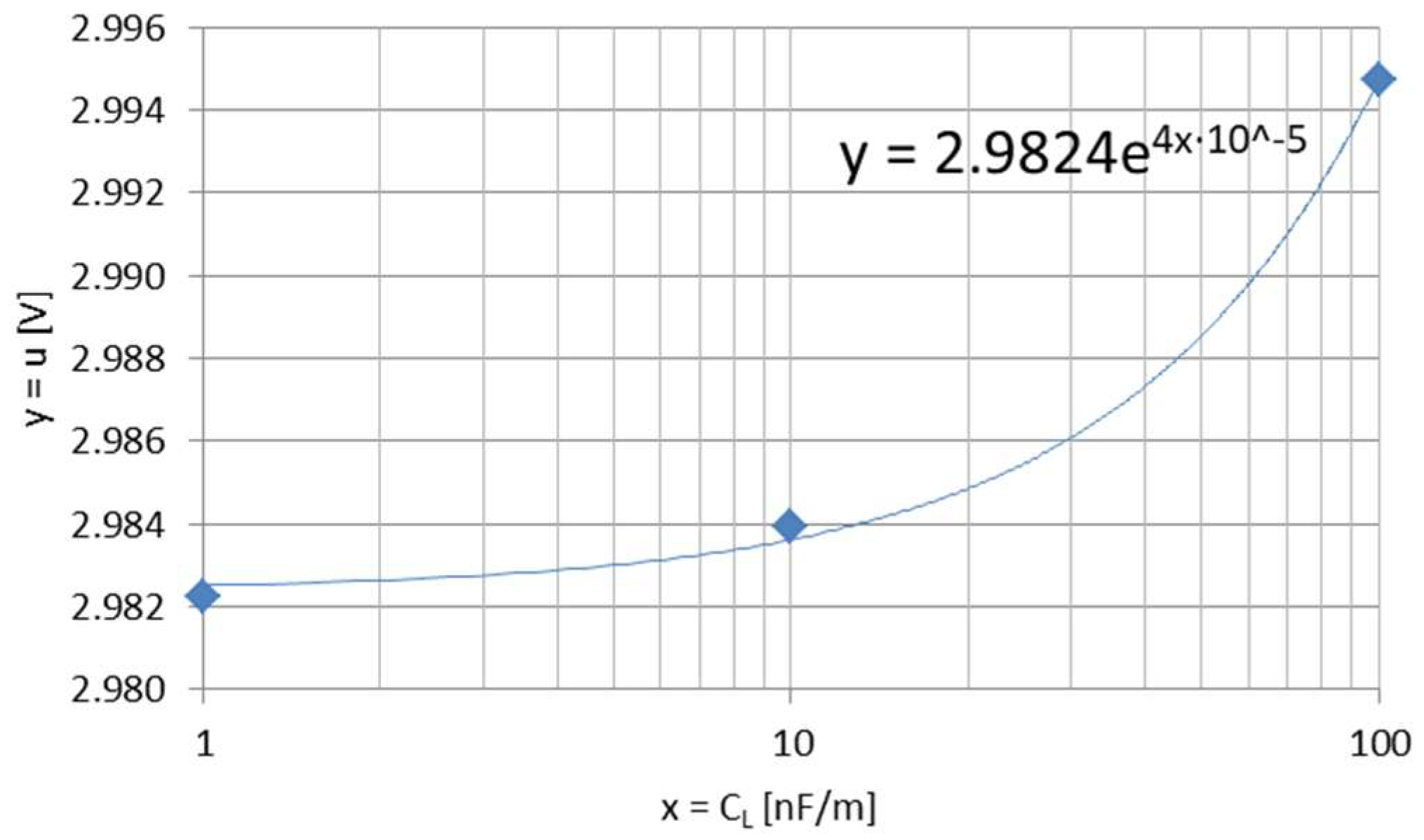
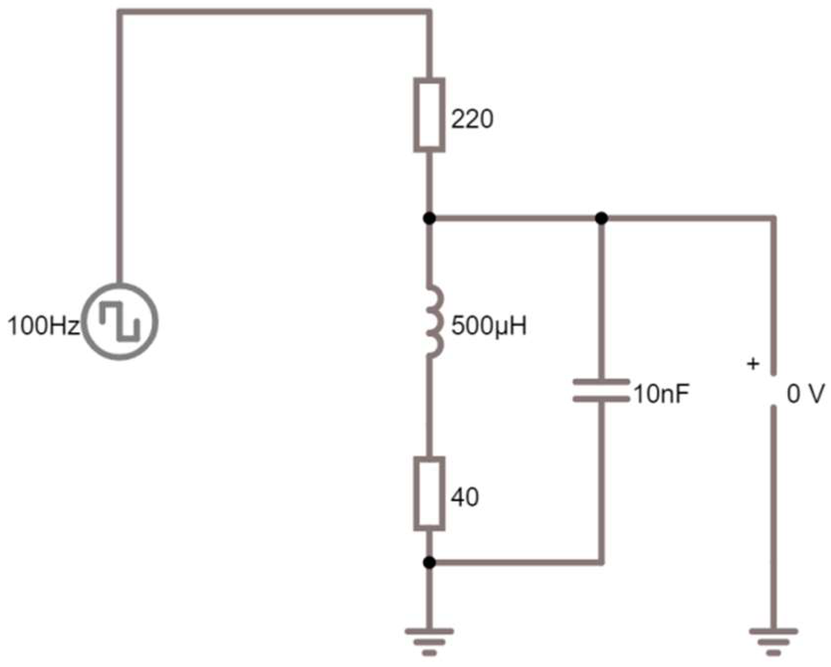
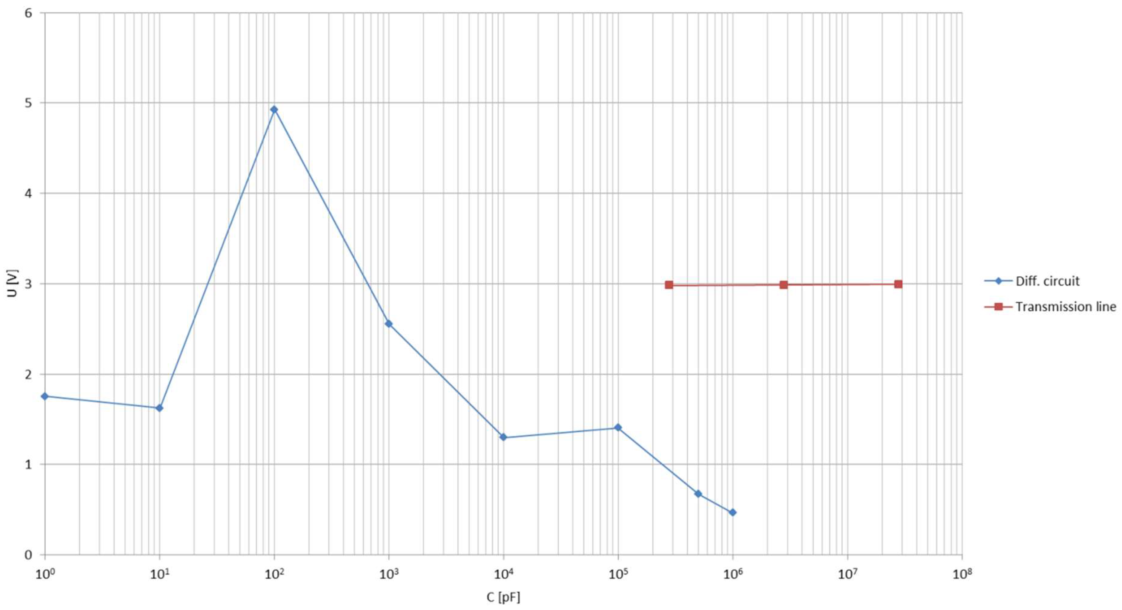
4.2. Transmission Line Model

Associating the behaviour of the measured inductance of the stealth magnetic loop to the presence of water in the wire’s surrounding environment requires the definition of a physical mechanism which, employing the water properties, such as the temperature and electrical permittivity (both co-dependent [26]), would explain the changes occurring in the measured values. In order to do so, the process of inductance measurement by the digital meter needs to be investigated.

A digital meter defines the inductance of the connected magnetic loop as a value proportional to the duration of the logic positive signal (‘one’), triggered by the occurrence of voltage above a certain level. This decaying voltage is an output product of a differentiating circuit, composed of the measured inductance and an internal meter’s resistor, excited by the digital meter’s internal square signal generator. The higher the value of the time constant τ of the differentiating circuit, the higher the value of the inductance [27]. AX-588B probes the circuit with a non-negative square signal of 100 Hz and the maximum voltage of 3 V [20]; the final product of the measurement is therefore dependent on the operation of the meter’s differentiating circuit and the functioning of the wire as a lossy transmission line, excited at a certain frequency [5,28]. Both of these actions are then dependent on the capacitance of the wire, directly linking the measurements with the changes in the electrical permittivity of the surrounding environment from the antenna point of view, and similarly to the phenomenon of parasitic capacitance in magnetic loops–only on a microscopic scale, with regards to the operating/measurement frequency and the dimensions of the loop [29].

The transmission line model is depicted in Figure 8: a lossy transmission line, excited with a function u(t,x) (voltage [V] dependent on time t [s] and the wire length x [m]), with its behaviour described by a telegrapher’s equation formulated as [28,29]:

$$L_L{C}_L\frac{{\partial }^{2}u\left(t,x\right)}{\partial t^2}+\left(L_L{G}_L+R_L{C}_L\right)\frac{\partial u\left(t,x\right)}{\partial t}+R_L{G}_{L}u\left(t,x\right)=\frac{{\partial }^{2}u\left(t,x\right)}{\partial x^2}$$

(1)

where L_L is the wire inductance in H/m; C_L is the capacitance between the signal and return conductors in F/m, with the water presence and flow affecting its value; G_L is the conductance (or leakance) in S/m; R_L is the resistance in Ω/m [30].

The equation was solved using Matlab software and an ODE45 embedded function, using x_max = 278 m, f = 100 Hz, h_max (max. value of the exciting square function) = 3 V, h_min (minimal value of the exciting square function) = 0 V, L_L = 1.8 μH/m (mean measured inductance divided with total wire length), R_L = 0.144 Ω/m (mean measured value of resistance divided with total wire length), G_L = 1 pS/m (value arbitrarily chosen) and C_L ranging from 1 to 100 nF/m (similarly to the value order of magnitude in [31]).

The results of the calculation are shown in Figure 9, with the achieved voltage values measured at the ends of the wire plotted in Figure 10. The differences in the voltage values were very little, and as the wire length was by design extremely disproportionate to the wavelength of the exciting square signal, its modified characteristics as a transmission line for given capacitances—showing clear resemblance to a short-circuited transmission line, yet completely disproportionate to the exciting frequency to show any structured voltage courses, depending on the changed parameters [28]—appeared to play a negligible role in affecting the measurements used by the meter to define the inductance of the loop (despite the variations in the capacitances over 2 degrees of magnitude). Therefore, the differentiating circuit of the digital meter requires deeper investigation.

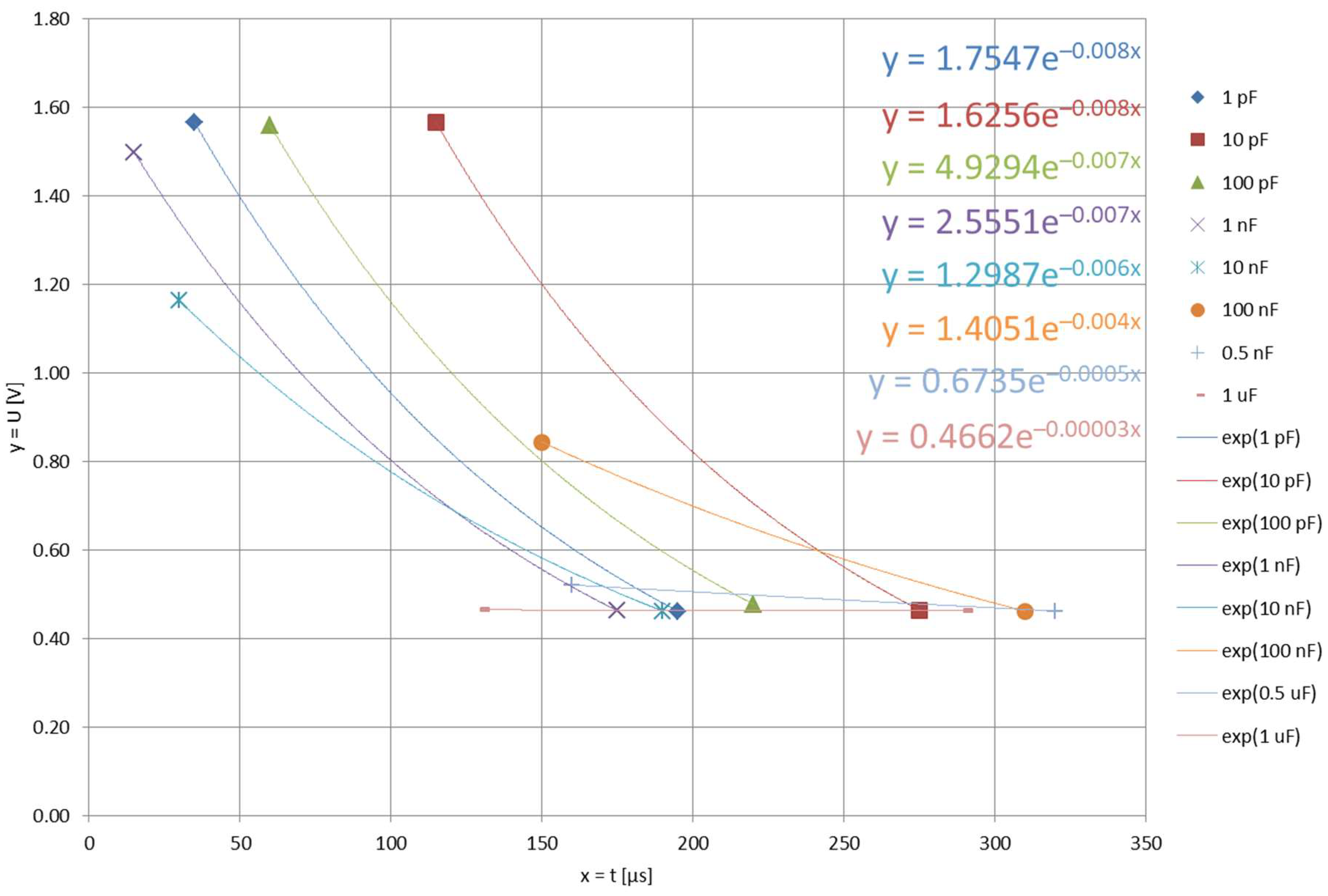
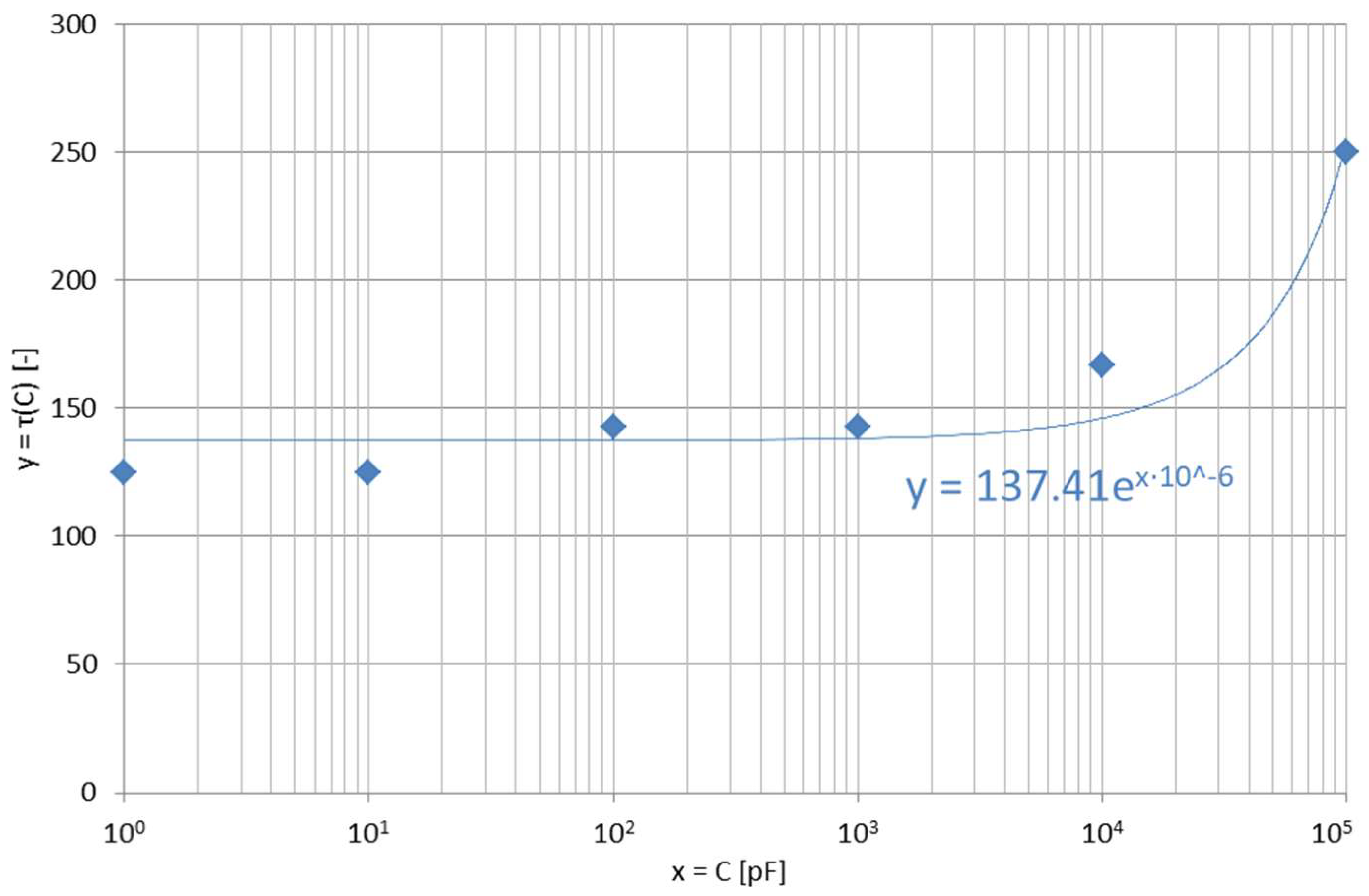
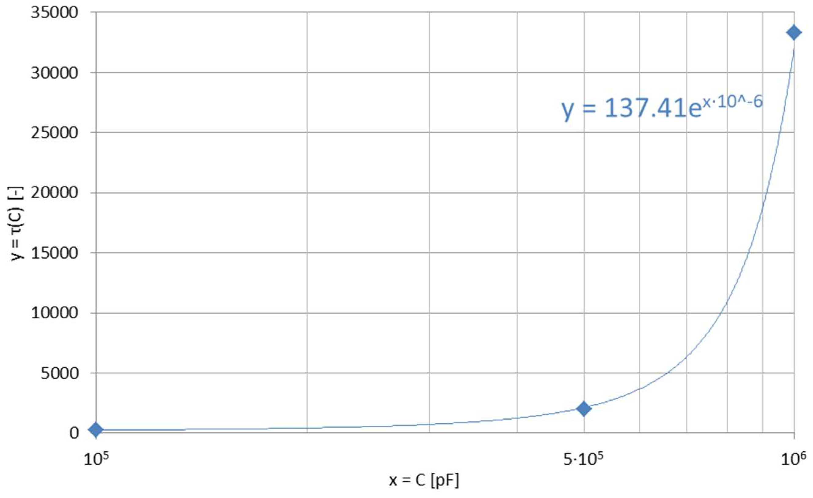
4.3. Differentiating Circuit

The differentiating circuit of the digital meter in this type of measuring device, excited with a square wave of the same parameters described in the previous section, was composed by design of the directly connected measured magnetic loop, its parasitic capacitance (in this case, dependable on the environmental conditions) and the meter’s internal resistor. As the details of the resistor inside AX-588B are not known, an exemplary value from similar designs of 220 Ω was adopted in the calculations [27] to show the overall functioning of the circuit and its susceptibility to changes in its parameters. The differentiating circuit was modelled and investigated in Falstad Circuit software; the schematic is shown in Figure 11. The ideal loop was expanded with its real DC resistance (40 Ω) and the parasitic/environmental capacitance, which was the changed value.

The voltage meter indicated the voltage output of the circuit as a function of voltage in time—this function was subject to change with the changed capacitance, as the ideal RL series circuit was transformed into an RLC parallel circuit with different time constant τ [s]. The capacitance values were swept from 1 pF to 1 μF, and for each capacitance value, a set of points (t; u) was read from the Falstad Circuit simulator; these points were then plotted (as shown in Figure 12) and approximated with exponential functions. These functions incorporated the 1/τ constants; Figure 13 and Figure 14 show these constants inverted and plotted against respective capacitance values.

From the approximated exponential functions shown in Figure 12, maximum initial values of the voltage (t = 0) can be calculated and plotted with similar data from the Matlab transmission line simulation—using both data sets for respective capacitance values. This comparison is shown in Figure 15, with the C_L [F/m] values recalculated to C [F] using the wire’s length of 278 m. This comparison (especially between 10⁵ and 10⁶ pF) clearly shows that for the digital meter’s operating frequency of 100 Hz, the parameters of the antenna considered as a transmission line remained almost unchanged, while the differentiating circuit providing voltage levels for inductance calculation appeared highly sensitive to parasitic capacitances, therefore giving different values for the measured/indicated inductance, which—if the parasitic capacitance is considered a variable— overall corresponded to the recorded longtime measurements. The maximum (in this data set) voltage value at 100 pF is most likely linked to the proximity to the resonance of the differentiating circuit as a whole (including the meter’s internal resistor).

As the presented approach to the differentiating circuit clearly showed a strong dependance on the environmentally-linked capacitance (in comparison to the presented transmission line model, which can be practically discarded from further investigation), an investigation into the parameters of this circuit can be performed in order to further characterise its susceptibility in the impedance and frequency ranges, separate from the already presented voltage response range. If the measured magnetic loop is considered as an RL (resistive-inductive) series circuit (no parasitic capacitance) and as an RLC (resistive-inductive-capacitive) circuit with parallel parasitic C (capacitive) branch, the impedances of these circuits can be calculated and compared. Formulas for the impedances are given as follows [32]:

$$Z_{R+L}=\sqrt{R^2+4{\pi }^2{f}^2{L}^2}$$

(2)

$$Z_{R+L\left|\right|C}=\frac{1}{\sqrt{{\left(\frac{R}{R^2+4{\pi }^2{f}^2{L}^2}\right)}^2+{\left(2\pi fC-\frac{2\pi fL}{R^2+4{\pi }^2{f}^2{L}^2}\right)}^2}}$$

(3)

The resonant frequencies of the RLC circuit can be defined as [32]:

$$f_{res.}=\frac{1}{2\pi }\sqrt{\frac{1}{LC}-{\left(\frac{R}{L}\right)}^2}$$

(4)

and for the mandatory requirement:

$${\left(\frac{R}{L}\right)}^2\ll \frac{1}{LC}$$

(5)

Figure 16 and Figure 17 show the impedances plotted against swept capacitance values for two different frequencies: 100 Hz (probing frequency) and 270 kHz (transmission frequency used in the IGLUNA 2019 experiment [15]). It can be seen that for higher frequencies, the occurrence of parasitic capacitance in the considered ground magnetic loop antenna can severely affect the impedance of the circuit, which, for higher powers, may cause issues with the antenna matching and the overloading of the power stage of the employed transmitter. The values of these capacitances are environmentally based, so certain environmental conditions (humidity, temperature—compounded with the properties of the soil around the wire) may form a frequency region where the operation of the magnetic loop as a transmitting antenna is highly unstable and presents risks of transmitter mismatch/overload (especially if higher powers are used).

Figure 18 presents the resonant frequencies, calculated using formula (4) when condition (5) is true, plotted against the capacitance values considered earlier. It can be noted that the ideal loop resonated in a very wide range of frequencies, ranging from hundreds of Hz up to 7 MHz. The environmental changes resulting in a change in the loop’s parasitic capacitance may easily and significantly alter this frequency, causing issues when operating in broadcasting mode; this phenomena, however, can be exploited for more detailed monitoring of a certain capacitance (by resulting voltage responses, causing instabilities in the measured inductance) linked to a defined environmental condition. Such a condition is expected to be linked to the electrical permittivity of the surrounding medium (as the overall geometry of the system remains stable, as mentioned in Section 4), which directly influences the parasitic capacitance, in turn affecting the differentiating circuit of the measuring device. This phenomena may be temperature- and humidity-dependent; these factors can be interdependent as well. To investigate this, a deeper investigation into the electrical permittivity must be performed.

4.4. Approach for The Electrical Permittivity

As the parasitic capacitance of the considered magnetic loop is directly dependant on the electrical permittivity of the surrounding medium (the soil), this parameter requires careful analysis in order to estimate the range of capacitance value changes (resulting finally in measured inductance changes) it may cause.

In the general approach, the permittivity of soil itself is practically independent of its density, granulation and temperature [33]; on the contrary, the electrical permittivity of water changes with its temperature [26,33]. If a soil is a mixture of different phase compounds (rocks, air, etc.), the total value of electrical permittivity can be defined as a function of the permittivities and the contents of subsequent phases (with the gaseous phase usually neglected due to lack of research). This approach, however, does not deliver sufficiently quantitative data [33]. From a measurement point of view, the electrical permittivity of dry and wet soil remains constant below ~200 MHz [34,35]. The exact values of the permittivity vary with the soil type/composition and its relative humidity (m³ of water per m³ of dry soil) [33].

To directly link the electrical permittivity of the medium with the capacitance (in three dimensions), a formula for a spherical capacitor can be used in the simplest approach, with the radius of the external sphere orders of magnitude higher than the radius of the inner sphere [33]:

$$C=4\pi {\epsilon }_0{\epsilon }_r{r}_{ext}$$

(6)

where ε₀ is the vacuum permittivity (8.854187817 × 10⁻¹² F/m [34]), ε_r is the electrical permittivity [–] and r_ext [m] is the radius of the external sphere of the capacitor; its value is chosen in a way which allows for the calculation of the electrical permittivity value for pure water, when pure water is present in the investigated sample (no soil)—it has been defined as 0.0796179 m [33].

Among many different sets of experimental data retrieved from various types of soil samples, the one most suitable was chosen as having the soil density the closest to the dry soil density occurring at the experimental setup of the magnetic loop antenna (~938 kg/m³, approximately 1 Mg/m³). In these data sets, the electric permittivity of the sample does not decrease with an increase in water content [33].

For the previously used set of capacitance values, the corresponding electrical permittivity was calculated using formula (6) and compared with generalised permittivity values for a soil sample described in [33]—the comparison is plotted in Figure 19, concentrating on the intersections of constant permittivity values with the calculated permittivity function. In can be noted that the entire range of electrical permittivity values for the chosen soil sample was covered between 300 and approximately 710 pF. This range can be therefore considered as the capacitance value range expected when operating in the presence of dry, wet and very wet light (1 Mg/m³) soil, if the model described by formula (6) is maintained.

To directly link the changes in the electrical permittivity of the soil with the recorded changes in measured inductance, two variables must be defined from other sources or further, deeper research: the electrical permittivity of a soil sample or samples (covering a larger area within the antenna’s aperture to provide a generalised/averaged value) and the set of precise parameters of the differentiating circuit of the measuring device (i.e., the precise value of the internal resistance). If those two variables are known, the precise calculation of the capacitance and electrical permittivity of the antenna’s surroundings shall be possible.

As for the current amount of data, the expected electrical permittivity range of the soil, resulting in 300–710 pF of capacitance (dry-to-very humid range), would result (Figure 13) in time constants of the circuit equal to 0.0072664 and 0.0072335, which amounts to a relative drop of ~0.45% for the rising capacitance. As mentioned in Section 4.2, the higher the value of the time constant, the higher the indicated inductance; in this case, the relative differences of the mean inductances (for the same/similar temperatures—Figure 22) possessed the same degrees of magnitude as the relative drop in the time constant value. Therefore, this model (the differentiating circuit’s being sensitive to environmental changes) can be considered as actual and matched.

A natural difference between a laboratory-analysed soil sample and the experimental setup of the magnetic loop antenna, laid directly on the ground, includes the boundary conditions of the influence of the surrounding environment on the parameters of the antenna operating at a defined frequency (probing/measuring of transmitting). In the formula (6), a generic condition of a large capacitor was introduced; however, the external maximum dimensions of this capacitor can be limited using the radius of the near-field (or Fresnel) zone around the antenna and the skin depth, which describes the maximum penetration distance of the emitted electromagnetic wave through a medium of defined physical parameters. The Fresnel zone radius can be formulated as [28]:

$$r_{Fresnel}=0.62\sqrt{\frac{D_{max.}^3}{\lambda }}$$

(7)

where D_max. [m] is the maximum physical dimension of the antenna system (here defined as the longest diagonal of the antenna’s aperture, equal to 78 m) and λ [m] is the wavelength of the probing/transmitting signal.

The skin depth can be defined as [36]:

$$\delta =\sqrt{\frac{1}{\pi f\sigma {\mu }_0}}$$

(8)

where f is the frequency [Hz], σ is the conductivity of the ground [S/m] and μ₀ is the vacuum permeability, equal to 4π × 10⁻⁷ N/A² [34].

The differences between r_Fresnel and δ can be seen in Figure 20; at a certain frequency, the signal was able to penetrate the ground deeply, but the near-field zone—where the physical parameters of the loop core/surrounding medium were expected to cause the most significant influence on its parameters – was much smaller.

Both r_Fresnel and δ are plotted in Figure 21 as functions of operating frequency and various values of σ, respectively, representing different types of soils/surroundings. These values are, however, generic [9], and, especially for the rocky substrates, can vary even in many degrees of magnitude [37]—careful investigation of the exact soil type must therefore be carried out before applying these functions. The operating frequency range of the ground-laid magnetic loop as an environmental remote sensing tool for the wide-range investigation of soil parameters lies before the intersection of r_Fresnel and subsequent δ (f, σ) functions; the approximate maximum frequencies of such operations are: 62 kHz for rocks, 110 kHz for soils, 152 kHz for fresh water, and above 1 MHz for glacial ice. Above these frequencies, the emitted electromagnetic waves may be subjected to reflections, which could be useful in the transmissions or remote sensing of deep ground layers. Naturally, the radiation aspects of monitoring the antenna surroundings at higher frequencies must be taken into account when planning the experiments (from a physical and a legal point of view).

For the frequency of 100 Hz employed in the described experiments, the total amount of soil with absorbed water, enclosed in the antenna’s Fresnel region, was equal to approximately 35.910 t.

5. Results

In order to completely define the described antenna’s sensitivity to the surrounding environmental conditions, apart from the electrical permittivity, more parameters had to be included, i.e., the air temperature during the measurements (recorded as one of the parameters) and the amount of water in near proximity to the antenna. The temperature of the air, delivered in this region by EUMETSAT, was chosen as it was more uniform on the antenna aperture than the temperature of the ground or the temperature measured in the proximity of the building, as these may locally vary in different locations along the antenna aperture (due to the local presence of vegetation, local water accumulation or daily changes in insolation).

The measurements presented in Figure 3 have been regrouped using, simultaneously, recorded temperature and qualitative data on the humidity/water/snow present during the measurements. The rearranged sets of data are shown in Figure 22 (mean inductance values) and Figure 23 (ranges of inductance values).

In both Figures, three basic regions can be specified:

•

A snow region, with a recorded intense presence of snow and temperatures lower than 1 °C;

•

A water region, with recorded intense rain precipitation for temperatures above 1 °C;

•

A light water region, with recorded low rain precipitation for temperatures above 1 °C.

The fourth function groups’ data were classified as ‘drought’, where no specific precipitation was present.

Each of the three humid regions had their own function assigned, which approximated the changes in the parameters (mean inductance—mean L [mH], and the range of inductance values—ΔL [mH] in temperature T [K]). These parameters kept their original tolerance of indication, ±2.5% [20].

For the mean L:

•

The snow region: −5 × 10⁻⁴ T + 0.4969;

•

The light water region: 3 × 10⁻⁴ T + 0.4962;

•

The water region: −10⁻⁴ T + 0.4999.

For the ΔL:

•

The snow region: −2 × 10⁻⁴ T + 0.0144;

•

The light water region: 4 × 10⁻⁴x + 0.0315;

•

The water region: 10⁻⁵x + 0.0286.

For convenience, the functions have been repeated on Figure 22 and Figure 23.

6. Discussion

For the snow region, the tendencies on both Figures are similar—the mean L value and L range decreased with the increase in the temperature. For the water region, the mean L value dropped in comparison with no precipitation, but the L range increased significantly. The light water region appeared as transient, generally approaching the tendency present in the water region. The ‘drought’ data set for the same range of temperatures as the ‘light water’ range appeared more unstable for the mean L values, but generally approached the ‘light water’ data set for the L range.

The mean inductance values appeared to converge to certain approximated linear functions with the increases in water and snow presence. The drop in the mean inductance value can be seen for the increase in liquid water in the environment, which agrees with the general approach [33]; for snow (and ice), however, their electrical permittivity may have increased with the temperature drop [38], resulting in an overall increase in inductance measurements, which was confirmed on the plot. The inductance ranges were lowest for the highest concentrations of snow and water, with the highest values recorded for moderate amounts of water and moderate temperatures. This may correspond to the increased mobility of the liquid phase, both in the microscopic and macroscopic approaches, in the environment around the antenna—this mobility may distort the capacitive structures in the ground (water residues, water micro-flows, etc.), which results in the instability of the measured parameters. The mobility dropped with temperature, and led to water freezing, and the increase in temperature led to water evaporation.

6.1. Comparison to IGLUNA 2019 Glacier Antennas

As the exploited experimental loop antenna shares part of its technical/design details with the IGLUNA 2019 experimental antennas [15,17,18], a comparison between these two experiments can be carried out.

The IGLUNA 2019 experimental campaign employed two 278-m-long loop antennas, located on and inside the Klein Matterhorn glacier in Switzerland (3383 m a.s.l.). The inductances of these antennas were measured on a daily basis using the same digital meter from the previously described experiments [15]. The measured inductance ranges are shown plotted in Figure 24, based on the original data sets; the plotted mean inductance values can be found in [15]. The data referred to as ‘Glacier surface’ remain shorter and discontinued due to the damage to the antenna.

The antenna located inside the glacier was immersed in glacial ice with local small areas of liquid water; the air temperature in that environment was kept at a constant level of −5 °C. These parameters allow for a direct comparison between the measured inductance ranges of IGLUNA 2019 and the newly deployed magnetic loop antenna. For the first one (Figure 24), the mean ΔL value was equal to 0.014; for the second one (Figure 23), the mean ΔL value was equal to 0.0154, which indicates a very good match of the cold ‘snow region’ with the conditions inside the glacier (humidity, temperature), which is consistent with reality. The mean inductance values measured inside the glacier remained mostly constant, which indicates a stable and water-rich environment, and this is consistent in tendency with the ‘water region’ defined in Figure 22. The surface antenna—a cable formed by a bundle of wires, laid on the glacier surface—was subjected not only to mechanical damages, but also to high amplitudes of temperatures and changing amounts of accumulated ‘snow’ in the form of tiny ice crystals. These factors may have caused the mean inductance values and the inductance ranges to vary intensively, but a lack of additional data (for example, detailed weather reports) make this element of the analysis impossible.

6.2. Comparison to Homer Tunnel Antenna Experiments (1993)

In 1993, a large vertical magnetic loop antenna was deployed in New Zealand, using a mountain and a tunnel below it as supportive structures [14]. The mountain core of the loop remained solid; the antenna measurements, performed in different weather conditions (light rain and heavy rain) and using a different method than that described in the above experiments, showed that the reactance of the loop antenna changed intensively for frequencies above ~15 kHz, especially in the region where the antenna showed series resonance.

Table 1. Reactance values’ changes measured in the Homer Tunnel antenna experiment [14].

Condition	f [kHz]	X [Ω]	L [H]
Heavy rain during measurements	19.42	1580	0.01294875
Rain day before measurements	21.36	2252	0.01677982
No rain for 2 weeks before measurements	21.36	2910	0.02168263

presents frequency values for this resonance for different environmental conditions.

The increase in measured inductance was noted for the decrease in humidity around the antenna—this is consistent with the dependencies shown in Figure 22. The authors of [14] also noted that their results were consistent with older experiments carried out by Fenwick and Weeks in 1963 [5], where a long horizontal dipole was laid on the ground and measured during different weather conditions. The consistency of these results is also worth noting considering the fact that the test dipole antenna in 1963 was analyzed as a transmission line, with the water layers/presence acting as the return conductor, which is substantially different from the approach in 1993 [14] and in this work. Despite this difference, the similarities in the conclusions indicate that the environmental phenomena responsible for the changes in the measured antenna parameters are common and were identified equally correctly.

7. Conclusions

A magnetic loop antenna was built in 2020 and measured throughout 6 months in different environmental conditions. The conclusions from the analysis of the collected data can be summarised as follows:

•

For the given antenna dimensions and probing frequency, the method of measurement by the digital meter indicated that the variability of the measured inductance can be linked to the changes in the antenna’s parasitic capacitance, and therefore to the electrical permittivity of the surrounding medium;

•

An increase in the environment’s humidity caused the convergence of inductance measurements to a certain value in long-time measurements;

•

An increase in the environment’s humidity caused an increase in the range of the measured inductance;

•

The parameters of the ground, when investigated separately, can be directly linked to the capacitance changes they caused and, therefore, to the changes in the measured inductance;

•

The defined functions of changes of measured antenna parameters for the encountered environmental factors can be considered as boundary conditions, between which other (for example, less humid or vaporised) cases are to be allocated;

•

Developing a precise definition of the influence of electrical permittivity on the measured antenna parameters requires precise knowledge on the parameters of the measuring circuitry;

•

The dependencies described in this paper are consistent with previous experiments in different locations and setups.

The described antenna system can be easily adapted as an inexpensive, wide-range and remote tool for monitoring the environment for excessive amounts of accumulated and absorbed water, and can cover significantly larger areas than conventional methods/measuring arrays [39], delivering data used for example, for issuing early flood awareness warnings.

References

- Bosch, F.; Gurk, M. Comparison of RF-EM, RMT and SP measurements on a karstic terrain in the Jura mountains (Switzerland). In Proceedings of the Seminar ‘Electromagnetische Tiefenforschung’, Altenberg, Germany, 20–24 March 2000; Deutsche Geophysikalische Gesselschaft: Hamburg, Germany, 2000. [Google Scholar]
- Groundwater Geophysics: A Tool for Hydrogeology, 2th ed.; Kirsch, R. (Ed.) Springer-Verlag: Berlin/Heidelberg, Germany, 2009. [Google Scholar]
- Bem, D.J. Auxiliary Materials for Propagation Calculations; Wrocław University of Technology: Wrocław, Poland, 1974. [Google Scholar]
- Bem, D.J. Antenna Array in the Radio Broadcasting Centre Solec Kujawski (Polish Radio, JSC). Przegląd Telekomun. Wiadomości Telekomun. 2000, 8–9, 577–585. [Google Scholar]
- Fenwick, R.C.; Weeks, W.L. Submerged antenna characteristics. IEEE Trans. Antennas Propag. 1963, 11, 296–305. [Google Scholar] [CrossRef]
- Miś, T.A.; Modelski, J. Stratospheric VLF Vertical Electric Mono- and Dipole Antenna Tests in 2014–2015. In Proceedings of the 2018 Baltic URSI Symposium, Poznań, Poland, 15–17 May 2018; Volume I. [Google Scholar] [CrossRef]
- Miś, T.A. The concept of an airborne VLF transmitter with vertical electric dipole antenna. In Proceedings of the IEEE International Symposium on Antennas and Propagation and USNC-URSI Radio Science Meeting, Boston, MA, USA, 8–13 July 2018. [Google Scholar] [CrossRef]
- Wilson, D. Channel Characterization and System Design for Sub-Surface Communications. Ph.D. Dissertation, The University of Leeds, School of Electronic and Electrical Engineering, Leeds, UK, February 2003. [Google Scholar]
- Burrows, M.L. ELF Communications Antennas; Peter Peregrinus Ltd.: London, UK, 1978. [Google Scholar]
- Morgan, M.G. An island as a natural very-low-frequency transmitting antenna. IRE Trans. Antennas Propag. 1960, 8, 528–530. [Google Scholar] [CrossRef]
- Pickworth, G. VLF Earth loop Antennas. Part I. Electron. Today Int. 1991, 1, 30–32. [Google Scholar]
- Uzunoglu, N.K.; Kouridakis, S.J. Radiation of Very Low and Extremely Low Frequencies (VLF & ELF) by a natural antenna based on an island or a peninsula structure. Radio Sci. Bull. 2004, 2004, 7–12. [Google Scholar]
- Turczyński, Z.; Łakomy, W. Personal safety indicator for the detection of pre-fainting stage of the miners and others. Wiadomości Górnicze 1987, 1, 15–21. (In Polish) [Google Scholar]
- Barr, R.; Ireland, W. Low-frequency input impedance of a very large loop antenna with a mountain core. IEE Proc. 1993, 140, 84–90. [Google Scholar] [CrossRef]
- Miś, T.A.; Modelski, J. The Analysis of Experimental Deployment of IGLUNA 2019 Trans-Ice Longwave System. Remote Sens. 2020, 12, 4045. [Google Scholar] [CrossRef]
- Republic of Poland's Office of Electronic Communications. Document DC.WRT.5104.6.2020.6; Republic of Poland's Office of Electronic Communications: Warszawa, Poland, 21 July 2021. [Google Scholar]
- Miś, T.A. The design, development and demonstration of longwave communication system for lunar surface operations. In Proceedings of the SECESA Conference on Space System Engineering, Delft, The Netherlands, 30 September–2 October 2020; European Space Agency: Noordwijk, The Netherlands, 2020. [Google Scholar]
- Miś, T.A. The results of IGLUNA 2019 trans-ice longwave communication system tests. In Proceedings of the MIKON Conference, Warszawa, Poland, 5–8 October 2020. [Google Scholar]
- Miś, T.A. The performance analysis and optimization of IGLUNA 2019 lunar-analogue longwave transmitting system. In Proceedings of the Baltic URSI Conference, Warszawa, Poland, 5–8 October 2020. [Google Scholar]
- Digital Multimeter AXIOMET AX-588B. In User Manual; Transfer Multisort Electronic: Atlanta, GA, USA, 2018.
- Titow, W. PVC Technology; Elsevier Applied Science Publishers: London, UK, 1984. [Google Scholar]
- Kaczyński, N. Soil; PIWR: Warszawa, Poland, 1950. (In Polish) [Google Scholar]
- Wieczysty, A. Engineering Hydrogeology; PWN: Warszawa-Kraków, Poland, 1970. (In Polish) [Google Scholar]
- Falkowski, M.; Nowak, M.; Prończuk, J.; Ralski, E. Meadowing. Vol II: Meadow Management; PWRiL: Warszawa, Poland, 1970. (In Polish) [Google Scholar]
- Badru, R.A.; Adeniran, S.A.; Atijosan, A.O. Effect of magnetic field on charged water vapour in motion. Eur. J. Eng. Technol. 2015, 3. [Google Scholar]
- Rusiniak, L. Electric properties of water. New experimental data in the 5 Hz—13 MHz frequency range. Acta Geophys. Pol. 2004, 52, 63–79. [Google Scholar]
- Janeczek, A. Simple induction meter. Electron. All 2003, 50–51. (In Polish) [Google Scholar]
- Poisel, R.A. Antenna Systems and Electronic Warfare Applications; Artech House: Norwood, MA, USA, 2012. [Google Scholar]
- Bogdanov, A.F.; Vasin, V.V.; Dulin, W.N.; Ilin, V.A.; Krivitskiy, V.H.; Kuznietsov, V.A.; Labutin, V.K.; Molochkov Yu, B.; Piertsov, S.V.; Stiepanov, B.M.; et al. Radioelectronics—A Handbook. Volume 1; Kulikovski, A.A., Ed.; WKiŁ: Warsaw, Poland, 1971. (In Polish) [Google Scholar]
- Jeffery, J.E. Impedance control of conductors acting as transmission lines in printed boards for high-frequency digital applications. Circuit World 1997, 23. [Google Scholar] [CrossRef]
- Investigation of a Transmission Line; Częstochowa University of Technology, Division of Electrotechnology, WZET Laboratory: Częstochowa, Poland, 2019. (In Polish)
- Electron Tube Handbook. Vol. II; Brown, Boveri & Co., Ltd.: Baden, Switzerland, 1971.
- Usowicz, B. Statistical-physical models of mass and energy flow in porous environments. Acta Agroph. 2000, 29, 3–113. (In Polish) [Google Scholar]
- Recommendation ITU-R P.527–4. In Electrical Characteristics of the Surface of the Earth; ITU: Geneva, Switzerland, 2017.
- Electrical Permittivity Characterization of Aqueous Solutions. Available online: https://chem.libretexts.org/Bookshelves/Analytical_Chemistry (accessed on 1 February 2021).
- Fraser-Smith, A.C.; Bannister, P.R. Reception of ELF signals at antipodal distances. Interaction of electromagnetic fields of ELF controlled sources with the ionosphere and Earth's crust. Proc. All-Russ. Res. Pract. Workshop 2014, 1, 144–149. [Google Scholar]
- Gierlotka, S. Geomagnetic properties of rocks. Propuls. Steer. 2019, 1, 40–43. (In Polish) [Google Scholar]
- Finkyelshteyn, M.I.; Mendyelson, W.L.; Kutyev, W.A. Radiolocation of Layered Ground Covers; Sovetskoye Radio: Moskva, Russia, 1977. (In Russian) [Google Scholar]
- Guide on the measurements of conductivity. In Theory and Practice Of Measurement Execution; Mettler-Toledo Sp.z.o.o: Warszawa, Poland, 2013. (In Polish)