A Two-Round Weight Voting Strategy-Based Ensemble Learning Method for Sea Ice Classification of Sentinel-1 Imagery

Abstract

Sea ice information in the Arctic region is essential for climatic change monitoring and ship navigation. Although many sea ice classification methods have been put forward, the accuracy and usability of classification systems can still be improved. In this paper, a two-round weight voting strategy-based ensemble learning method is proposed for refining sea ice classification. The proposed method includes three main steps. (1) The preferable features of sea ice are constituted by polarization features (HH, HV, HH/HV) and the top six GLCM-derived texture features via a random forest. (2) The initial classification maps can then be generated by an ensemble learning method, which includes six base classifiers (NB, DT, KNN, LR, ANN, and SVM). The tuned voting weights by a genetic algorithm are employed to obtain the category score matrix and, further, the first coarse classification result. (3) Some pixels may be misclassified due to their corresponding numerically close score value. By introducing an experiential score threshold, each pixel is identified as a fuzzy or an explicit pixel. The fuzzy pixels can then be further rectified based on the local similarity of the neighboring explicit pixels, thereby yielding the final precise classification result. The proposed method was examined on 18 Sentinel-1 EW images, which were captured in the Northeast Passage from November 2019 to April 2020. The experiments show that the proposed method can effectively maintain the edge profile of sea ice and restrain noise from SAR. It is superior to the current mainstream ensemble learning algorithms with the overall accuracy reaching 97%. The main contribution of this study is proposing a superior weight voting strategy in the ensemble learning method for sea ice classification of Sentinel-1 imagery, which is of great significance for guiding secure ship navigation and ice hazard forecasting in winter.

1. Introduction

As an essential component of the Arctic environment and even the global marine environment, sea ice plays a critical role in the weather and global climate system [1]. It not only affects the dynamic conditions and heat exchanges between the ocean and atmosphere but also plays an important role in the climate and marine ecosystem [2,3,4,5]. Over the past three decades, the reduction in sea ice cover has not only had a profound impact on the climate, hydrology, and ecology of the Arctic region [6,7,8,9] but has also, to some extent, promoted the expansion of the navigation windows of the Arctic shipping routes with advantages in navigation costs and time costs, thus leading to the increase in maritime transport in the Arctic region [10,11,12]. However, even in summer, navigation has increased risks due to the presence of sea ice. In this regard, repaid acquisition of marine meteorological information including sea ice is crucial for ensuring the safety of navigation in polar regions. To this end, the International Maritime Organization (IMO) issued the Polar Code on 1 January 2017, in which ships passing through the polar regions must receive the latest ice information, mainly including the type, thickness, and concentration of sea ice [13]. The sea ice type can be defined according to the stage of sea ice development, from smooth nilas ice to deformed and rough new ice, and multi-year ice that has survived through the entire summer.

Remote sensing has become an important technological means for large-scale sea ice monitoring in the Arctic region due to its advantages of a wide detection range and rapid data acquisition. In particular, synthetic-aperture radar (SAR) has become an indispensable observation system in polar sea ice monitoring with its all-weather and all-day advantages. Moreover, as SAR signals of different frequencies differ in their abilities to penetrate into sea ice, multi-band SAR contributes to capturing the complementary information of sea ice [14]. To be specific, L-band (1~2 GHz) SAR has higher penetration into wet snow and sea ice and can provide internal structural information of sea ice, such as thickness, salinity, and distribution of the bubbles [15,16]. That is, L-band SAR has more advantages in identifying the types of melting sea ice but tends to confuse new ice with open water [17]. On the contrary, X-band (8~12 GHz) SAR has a small penetration depth and is more sensitive to the increase in sea ice thickness during the early stage of sea ice growth. That is, X-band can distinguish new ice from multi-year ice but has a poor ability to distinguish gray ice from gray-white ice [18]. Up to now, most of the SAR sensors in service operate at the C-band (4~8 GHz), which is between the X-band and the L-band. Due to the moderate frequency adopted, the backscattering coefficients of different types of sea ice are significantly different in the C-band. That is the reason why C-band SAR has proved to be the most suitable sensor for polar sea ice type identification, especially for distinguishing ice from open water [19].

In recent decades, many representative semi-automatic and automatic algorithms have emerged and been applied in practice for sea ice classification of SAR images. These models include simple backscatter thresholding [20], clustering algorithms [21,22], expert systems [23,24,25], semantics segmentation (IRGS) [26], machine learning (support vector machines, neural networks) [27,28,29,30], and deep learning (CNN) [31,32,33]. Tan [26] proposed a semi-automatic sea ice classification algorithm for Sentinel-1 SAR images, which incorporated feature selection via random forest and iterative region growing using a semantics model to achieve multi-category sea ice classification in the Labrador Sea. Huiying Liu [28] proposed a method for sea ice classification based on the texture features and sea ice concentration of dual-polarization Radarsat-2 ScanSAR images. Six types of sea ice were classified including open water (OW), new ice (NI), leveled gray ice (LGI), deformed gray ice (DGI), second-year ice (SYI), and multi-year ice (MYI). Bogdanov et al. [30] compared neural networks with other supervised learning algorithms based on linear discriminant analysis (LDA) and used these algorithms to identify six sea ice types from RADARSAT and ERS SAR images of the Kara Sea. In addition, with the successful applications of deep learning models in image processing, preliminary explorations of these models have also been conducted in the classification of sea ice [31,32,33]. For instance, Hugo Boulze et al. [31] utilized a convolutional neural network (CNN) to recognize new ice, first-year ice, and multi-year ice based on 255 images of Sentinel-1 sea ice interpreted by experts. The recognition performance was better than the random forest algorithm, with the overall classification accuracy reaching 91.6%.

The above-mentioned classifiers can improve the classification accuracy of sea ice to a certain extent. However, the whole classification process mainly relies upon one single classifier, rather than combing the advantages of multiple different classifiers. To fully integrate the advantages of different classifiers, ensemble learning has been introduced into remote sensing image classification [34,35,36]. The most protruding characteristic of ensemble learning is the complementarity among the base classifiers. That is, when one classifier misclassifies some samples, other classifiers may correct the categorization of these samples. Therefore, the ensemble learning approach has great potential in improving the accuracy of image classifications. However, it is challenging to design an ensemble learning model with an excellent classification performance. To enhance the robustness of ensemble learning models, the voting strategy adopted herein deserves careful consideration.

Under this background, the concept of ensemble learning is introduced into sea ice classification for the first time. Meanwhile, this paper proposes an ensemble learning method based on a two-round weight voting strategy (TRWV) for the effective classification of sea ice using multi-temporal Sentinel-1 SAR images. Compared with the traditional ensemble methods, this study has the following main remarkable characteristics. During the first round of the voting stage, the weights of six base classifiers are optimized by using a genetic algorithm. After obtaining the first coarse classification result, pixels therein can then be identified to be fuzzy or explicit. The fuzzy pixels are further rectified based on the local similarity of the neighboring explicit pixels. The final precise classification result indicates that the proposed two-round weight voting strategy can significantly reduce the impact of speckle noise of SAR images. At the end, experiments are carried out on 18 scenes from Sentinel-1 SAR images from the Northeast Passage in the Arctic region. In addition, six base classifiers and four different voting strategies are employed as the comparisons, which fully validate the effectiveness and superiorities of the proposed method. The rest of this paper is organized as follows. Section 2 describes the proposed method, including data preprocessing and the detailed algorithm framework. In Section 3, the experimental results are presented and compared with other methods. Section 4 is devoted to the discussions and limitations. Finally, Section 5 concludes this study.

2. Methods

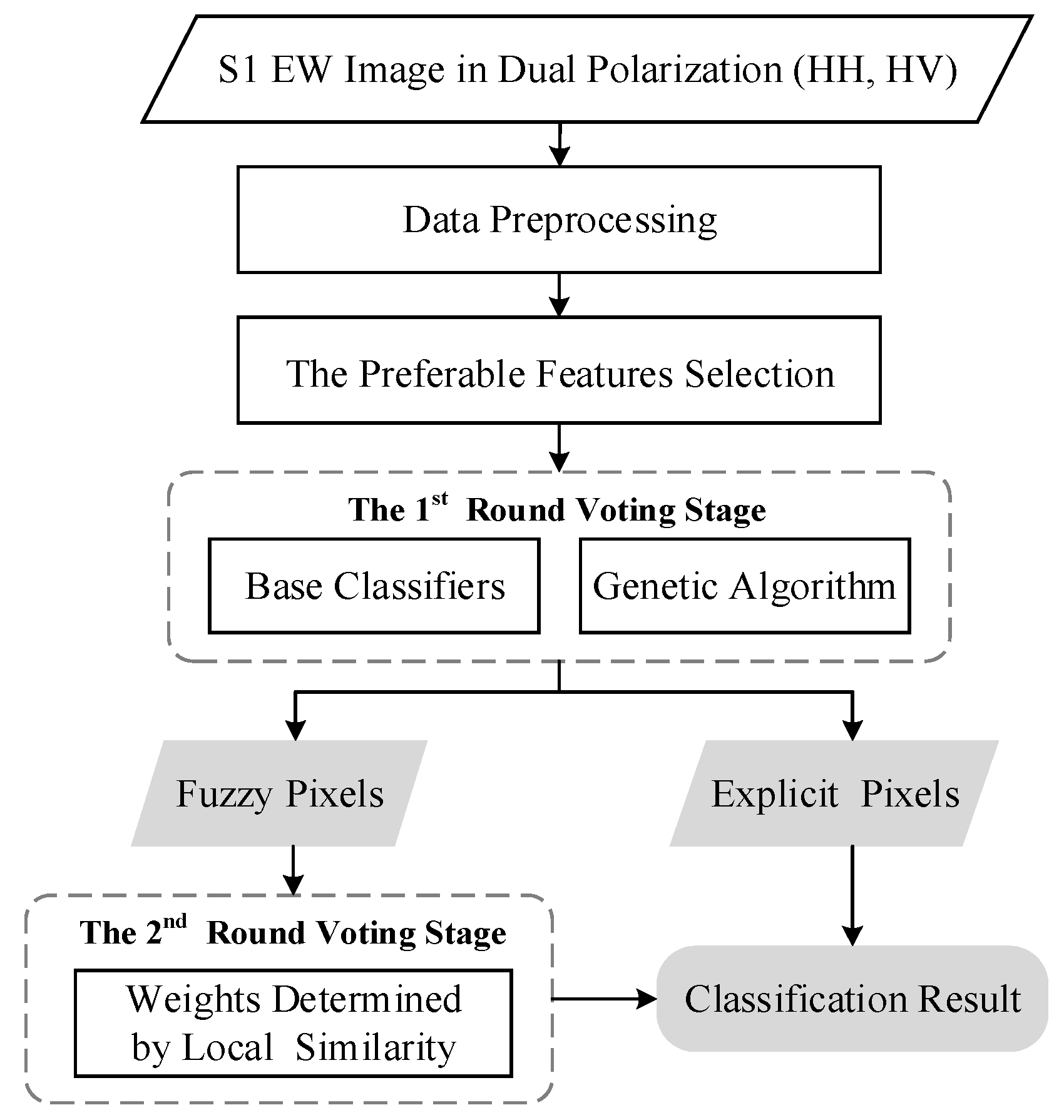
The overall architecture of the proposed TRWV method is depicted in Figure 1 for deriving sea ice categories from S1 EW images in HV and HH polarization. Firstly, the S1 EW images are preprocessed, which includes applying an orbit file, denoising, radiometric calibration, incidence angle correction, and converting to the decibel scale. Secondly, the preferable features of sea ice are selected via random forest from polarization features (HH, HV, HH/HV) and GLCM-derived texture features. Then, the weights of classifiers optimized by a genetic algorithm are adopted during the first round of the weight voting stage. Meanwhile, all pixels are divided into fuzzy pixels or explicit pixels (whose definitions can be found in Equation (7) in Section 2.3). Finally, the fuzzy pixels can be expediently rectified based on the local similarity of the neighboring explicit pixel during the second weight voting stage.

2.1. Preferable Features Selection

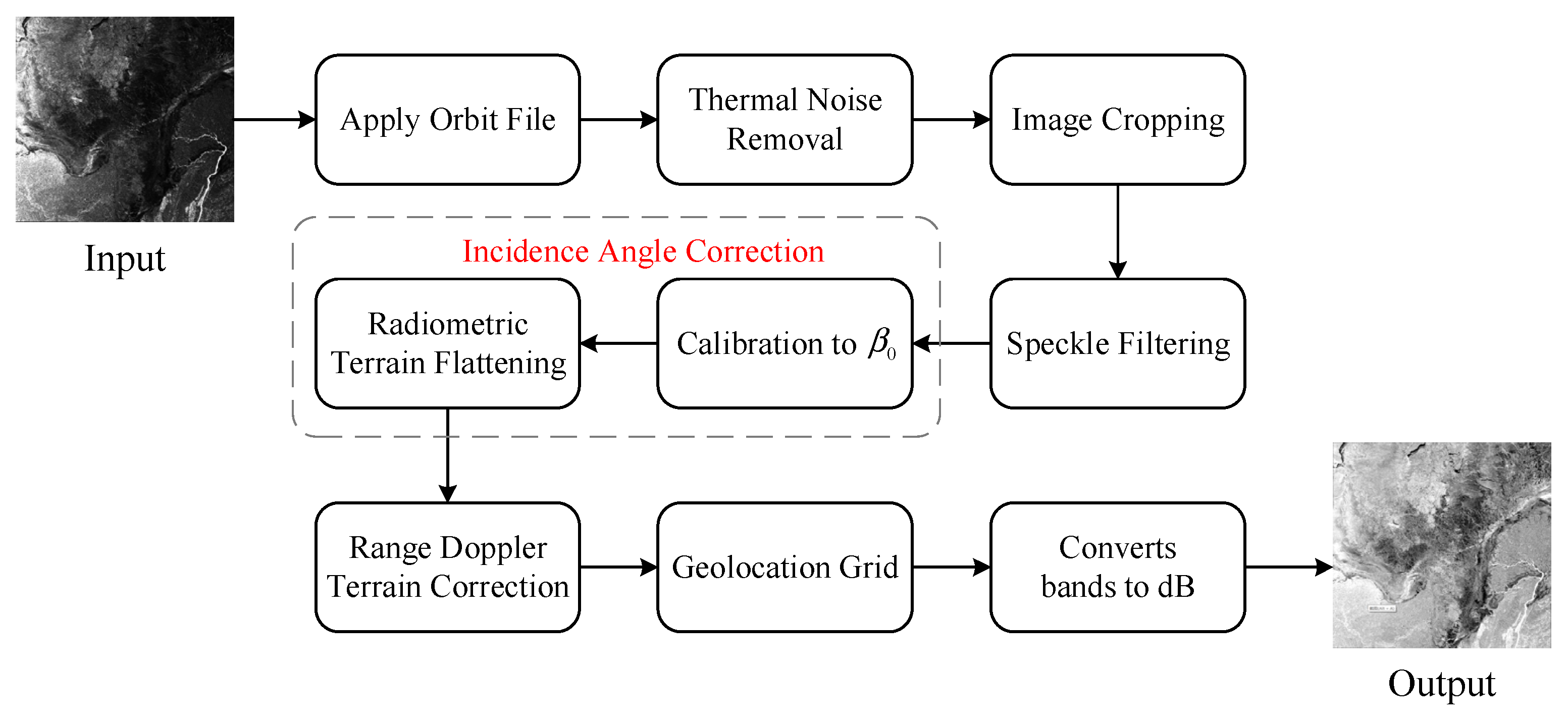
In this paper, Sentinel-1 EW dual-polarization (HV and HH) data were employed to verify the proposed algorithm. Some preliminary preprocessing was completed before the release of the S1 EW dual-polarized SAR data; however, it is still indispensable to perform further preprocessing work consisting of a series of standard corrections, which are the application of a precise orbit file, thermal removal, image cropping, speckle filtering, incidence angle correction, range Doppler and terrain correction, etc., for the proposed method. All these corrections in this paper were achieved mainly based on the SentiNel Application Platform (SNAP) [37] developed by the European Space Agency (ESA). The detailed procedures of the further preprocessing work are shown in Figure 2.

Numerous studies have shown that SAR sea ice classification performance is improved by using image texture features. The texture features describe spatial variations of the backscattering coefficients of a group of adjacent pixels in the SAR image. The most common and classic texture feature extraction method is based on the gray level co-occurrence matrix (GLCM) in sea ice classification. Since the GLCM is constructed according to the distance and direction of each pixel pair, it can synthetically reflect the micro-detailed and macro-expressed textures of sea ice.

The GLCM represents the probabilities of all pairwise combinations of gray levels within the window of interest. Normally, the GLCM textures are determined by four parameters: gray levels, the sliding window size, inter-pixel distance, and orientation. For each SAR sub-image constrained by a constant window size, the GLCM is calculated as follows [38,39,40]:

$$f_{d,\theta }\left(i,j\right)=\frac{P_{d,\theta }\left(i,j\right)}{{\displaystyle \sum _i^N}{\displaystyle \sum _j^N{P}_{d,\theta }\left(i,j\right)}}$$

(1)

where $f_{d,\theta }\left(i,j\right)$ is the GLCM value of a pixel pair; $P_{d,\theta }\left(i,j\right)$ represents the frequency number of grayscale “pixel pairs”; $i$ and $j$ appear simultaneously within the sliding window; $\theta$ is the observation angle involving 0°, 45°, 90° and 135°, which correspond to horizontal, northeast–southwest, vertical, and northwest–southeast, respectively; $d$ represents the distance between pixels, namely, the step size; $N$ denotes the gray levels.

In this study, GLCMs were calculated for ${\delta }_{HH}$, ${\delta }_{HV}$, and ${\delta }_{HH}/{\delta }_{HV}$ polarimetric SAR images. Therein, multiple window sizes and step sizes were thoroughly employed: window size 5 with step size 1, window sizes 7 and 9 with step sizes 1 and 3, and window size 11 with step sizes 1, 3, and 5. To reduce the computation amount, the gray levels of the image were compressed from 256 to 32. Furthermore, the extracted texture features were obtained by averaging the GLCM from four different angles. Here, we calculated ten texture measurements, which are the angular second moment (ASM), contrast, dissimilarity, energy, entropy, correlation, mean, variance, homogeneity, and maximum, resulting in a total of 240 candidate GLCM features. The detailed formula of these features can be found in [38,39]. These texture features were produced by the texture analysis module from SNAP. In addition, the extracted texture features, together with the foregoing 3 polarization features, were all normalized to the interval of [0, 1] for the convenience of subsequent experiments.

Due to the information redundancy among the extracted texture features, feature reduction is an essential technique for capturing the important features or feature combinations. Random forest is a widely adopted feature selection method because of its simple principle, easy implementation, and low computational cost. Its main idea is to combine a number of decision trees built from bootstrapped training samples using a random subset of features. During this process, the random forest provides the corresponding importance measurement for each input feature $f$ by the following Equation (2):

$$Importanc{e}_f=\frac{1}{n}{\displaystyle \sum }_{v\in S}F\left(f,v\right)$$

(2)

where $F\left(f,v\right)$ represents the importance of feature $f$ in decision tree $v\in S$, and $S$ is the set of all decision trees, $S=\left\{Tre{e}_1,Tre{e}_2,\cdots ,Tre{e}_n\right\}$. The importance of the random forest is described by the variation in the classification accuracy of the out-of-bag (OOB) sample, known as out-of-bag (OOB) error, which is caused by random transformation of features in the OOB sample. The function $F\left(f,v\right)$ in Equation (2) is given as follows:

$$F\left(f,v\right)=\frac{{{\displaystyle \sum }}_{x_i\in {\varphi }_{OOB}}N\left[l_i=c_i^v\left(f\right)\right]}{\left|{\varphi }_{OOB}\right|}-\frac{{{\displaystyle \sum }}_{x_i\in {\varphi }_{OOB}}N\left[l_i=c_i^v\left(f^{+}\right)\right]}{\left|{\varphi }_{OOB}\right|}$$

(3)

where ${\varphi }_{OOB}$ is the OOB sample set; $l_i$ represents the true classification label of pixel $x_i\in {\varphi }_{OOB}$; $c_i^v\left(f\right)$ is the category label of $x_i$ predicted by the decision tree based on the OOB dataset; $c_i^v\left(f^{+}\right)$ represents the predicted category label of pixel $x_i$ after random transformation of feature $f$; $N[\cdot ]$ counts the number of correctly classified samples.

The experiment of feature selection based on the random forest was carried out for 240 GLCM texture features on 16,124 artificially interpreted samples. The computation speed of the experiment and accuracy of the feature importance are mainly affected by two parameters: the number of decision trees and iterations. According to a previous study [41], 20 and 50 were set, respectively, in this experiment for the number of decision trees and iterations. Therefore, the ultimate importance according to each feature can be obtained by averaging the importance after 50 rounds of running the above experiment. By ranking each feature with its importance, the top six features were picked out as the representative features, presented in

Table 1. The top six co-occurrence matrix (GLCM)-derived texture features produced according to their averaged importance by random forest.

Polarization Image	Feature Name	Rank
${\delta }_{HV}$	Mean 7 × 7 Step 3	1
${\delta }_{HH}$	Correlation 11 × 11 Step 5	2
${\delta }_{HH}$	Mean 11 × 11 Step 5	3
${\delta }_{HV}$	Mean 5 × 5 Step 1	4
${\delta }_{HH}/{\delta }_{HV}$	Variance 5 × 5 Step 1	5
${\delta }_{HH}/{\delta }_{HV}$	Variance 11 × 11 Step 3	6

.

Moreover, to utmostly retain the SAR polarization information, the original 3 polarization features were also introduced, thereby aggregating the 9 preferable sea ice features. The flow chart of acquiring the preferable features of sea ice is shown in Figure 3.

2.2. The First Round Voting Stage—Coarse Classification

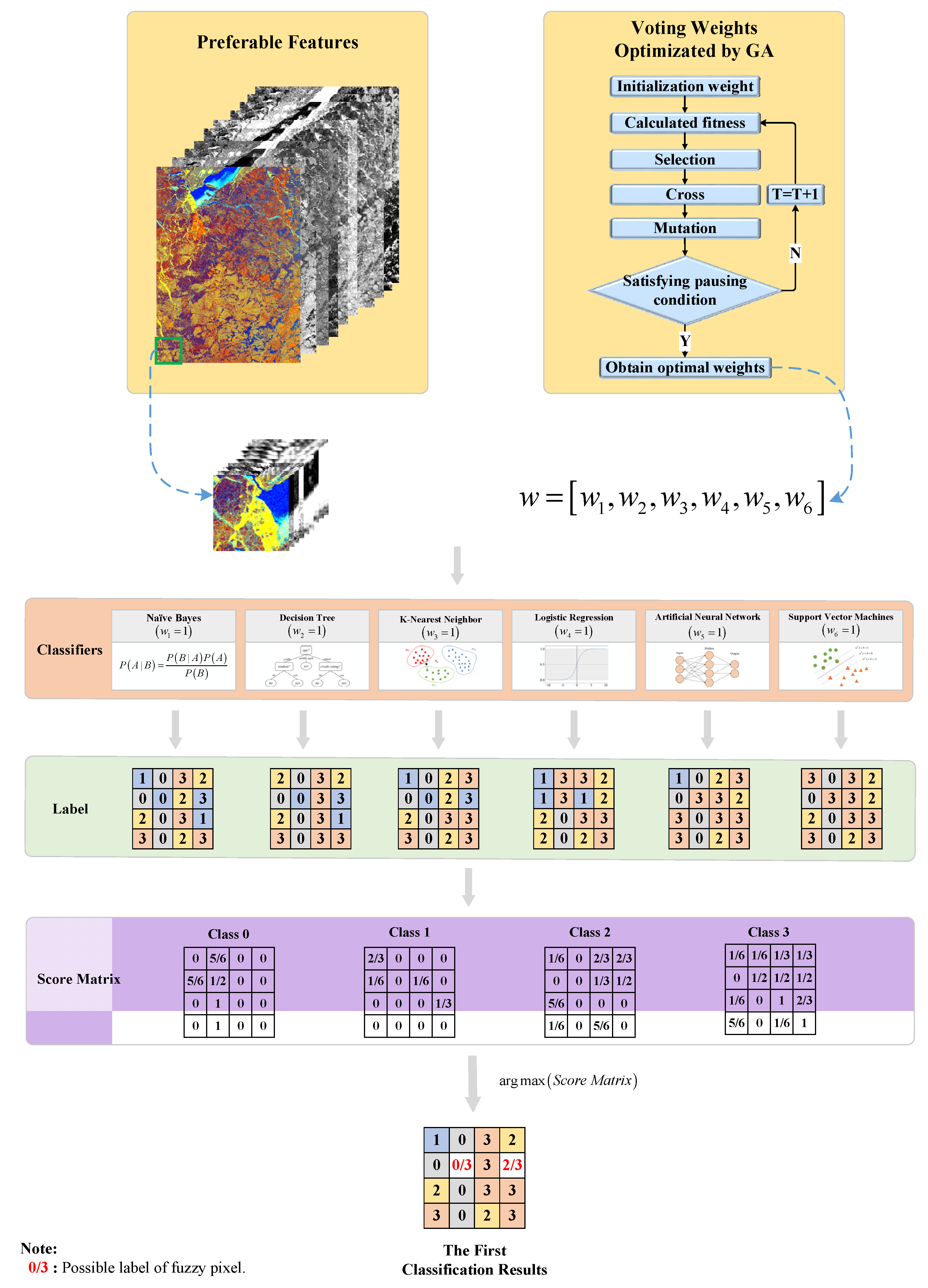
In order to fully integrate the advantages of different classifiers, ensemble learning has been introduced into remote sensing image classification [34,35,36]. In this paper, six frequently used classifiers, that is, naive Bayes (NB), decision tree (DT), k-nearest neighbor (KNN), logistic regression (LR), artificial neural network (ANN), and support vector machine (SVM), were employed as the base classifiers to generate the initial classification maps. Since the voting strategy plays a critical role in ensemble learning models, optimization of the voting strategy contributes to improving the classification ability of ensemble learning. Here, the voting strategy was improved with the voting weights of the base classifiers tuned by a genetic algorithm. Therefore, the first round voting stage was conducted on the initial classification maps to obtain the category score matrix and, further, the first coarse classification of sea ice. Figure 4 below illustrates the detailed process of the first round voting stage.

Specific descriptions of the six base classifiers (NB, DT, KNN, LR, ANN, and SVM) can be found in the literature [42,43,44,45,46,47]. Actually, the ensemble classification method operates by voting the initial classification results of different base classifiers according to a certain voting strategy. 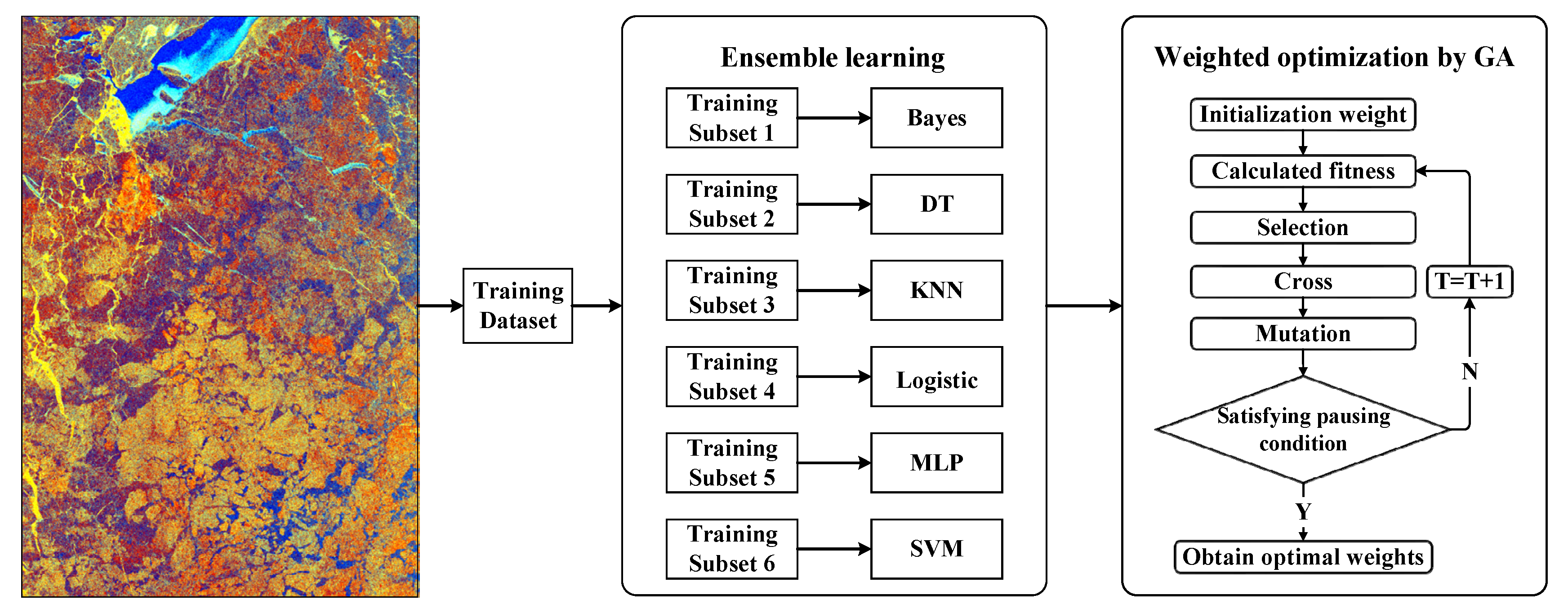At present, ensemble learning models are mainly implemented through the mechanisms of bagging [48], boosting [49], and stacking [50]. Here, the bagging mechanism is utilized due to its inherent majority voting concept being involved throughout, which improves the final classification by combining classifications of the base classifiers with randomly selected training data subsets. However, the selection of voting strategies has a significant impact upon the classification performance of the bagging mechanism. Here, the weighted voting strategy was employed, which assigns different weights to the classification results of different base classifiers to achieve the optimal classification. The weights of the above six base classifiers were optimized by a genetic algorithm (GA), whose algorithm flow is shown in Figure 5.

The specific steps of the GA are summarized as follows:

(1)

Initialization: A group of multiple individuals is randomly generated, and each individual represents the weight of each classifier.

(2)

Fitness: The GA computes the fitness (pros and cons) of individuals based on some objective evaluation function, thereby determining the survival probability of individuals in the next evolution.

(3)

Selection: A certain number of excellent individuals with “more fitness” are selected through random or specific population rules to participate in cross and mutation. Generally speaking, excellent individuals are usually of high fitness, that is, better classification performance can be expected if they are used as the weights of base classifiers.

(4)

Cross: New and excellent individuals are generated by exchange and combination of chromosomes.

(5)

Mutation: The individual diversity is increased through genetic mutation by randomly selecting some individuals with a certain probability.

Suppose $w=\left\{w_1,w_2,\dots ,w_T\right\}$ represents the weights of base classifiers, whose optimization process, as mentioned above, can essentially be formulated [51,52,53,54] as follows:

$$\{\begin{array}{l}{w}_{opt}=\underset{w}{\arg \min }{\displaystyle \sum _{j=1}^{m}Loss\left(L_{x_j},y_j\right)}\\ s.t.{\displaystyle \sum _{t=1}^T{w}_t}=1,0\le w_t\le 1\end{array}$$

(4)

where $L_{x_j}$ is the predicted label of the sample $x_j$. The loss function $Loss\hspace{0.17em}(\cdot )$ represents the difference between the predicted label $L_{x_j}$ and the true label $y_j$.

According to the optimized weights $w_{opt}=\left\{w_{opt}^1,w_{opt}^2,\cdots ,w_{opt}^B\right\}$ by the GA and the classification results of the base classifiers, the category score matrix of each pixel $\left(i,j\right)$ can be calculated as follows:

$$S_{i,j}^k={\displaystyle \sum _{b=1}^B{w}_{opt}^b\left(L_{i,j}^b=k\right)}$$

(5)

where $L_{i,j}^b$ represents the category label of the pixel $\left(i,j\right)$ predicted by the $b$th base classifier, and $S_{i,j}^k$ represents the category score value of this pixel assigned to category $k$, $k=1,2,\cdots ,K$ (the total number of categories).

Therefore, the maximum index of the category score can be calculated by the argmax function to obtain the rough classification label.

$$\begin{array}{ll}Labe{l}_{i,j}^{1st}& =\underset{index}{\arg \max }{S}_{i,j}\\ & =\underset{index}{\arg \max }\left\{S_{i,j}^1,S_{i,j}^2,\cdots S_{i,j}^K\right\}\end{array}$$

(6)

In other words, coarse classification of sea ice is achieved after the first round voting stage.

2.3. The Second Round Voting Stage—Precise Classification

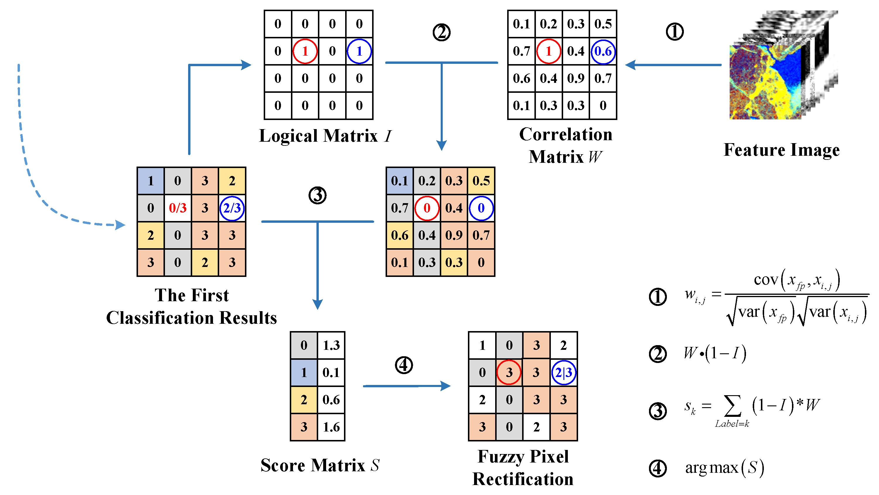
After the first round voting stage, the score values of some pixels assigned to different categories may be very close in the first coarse classification results. By introducing an experiential score threshold, each pixel can thus be identified as a fuzzy or an explicit pixel. As mentioned above, the fuzzy pixels are likely prone to be misclassified. To cope with this issue, the second round of voting is conducted to further determine the category attribution of the fuzzy pixels based on the local similarity of the neighboring explicit pixels, thereby yielding the final precise classification result. Figure 6 shows the process of the second round voting stage with the specific implementation steps described as follows.

Firstly, by using the category score matrix $S$ and the predefined threshold parameter $T$, each pixel can be identified as a fuzzy or an explicit pixel according to the following rules:

$$\{\begin{array}{l}Pixe{l}_{i,j} isFuz\mathrm{z}y Pixel,if \max \left\{S_{i,j}\right\}-2^{nd}\max \left\{S_{i,j}\right\}<T\\ Pixe{l}_{i,j} is Explicit Pixel,if \max \left\{S_{i,j}\right\}-2^{nd}\max \left\{S_{i,j}\right\}\ge T\end{array}$$

(7)

where $Pixe{l}_{i,j}$ represents the current pixel $\left(i,j\right)$ under consideration, and $\max \left\{S_{i,j}\right\}$ and $2^{nd}\max \left\{S_{i,j}\right\}$ represent the maximum and the secondary maximum of the category score vector corresponding to the pixel $\left(i,j\right)$, respectively. Therefore, a logical identification matrix $I$ is generated, indicating that each pixel is either fuzzy or explicit.

Then, for each fuzzy pixel, one corresponding matrix will be created depicting the similarities between the fuzzy pixel and its neighboring explicit pixels. These explicit pixels are all selected from such a square neighborhood centering this fuzzy pixel. Specifically, the correlation coefficient $w_{i,j}$ is introduced for depicting the similarity of the fuzzy pixel $x_{fp}$ and the explicit pixel $x_{i,j}\in N^m\left(x_{fp}\right)$ ($m$ represents the size of the neighborhood), which is calculated as follows:

$$w_{i,j}=\frac{\mathrm{cov}\left(x_{fp},x_{i,j}\right)}{\sqrt{\mathrm{var}\left(x_{fp}\right)}\sqrt{\mathrm{var}\left(x_{i,j}\right)}}$$

(8)

where $w_{ij}$ constitutes the similarity matrix $W$, and $\mathrm{var}\hspace{0.17em}(\cdot )$ and $\mathrm{cov}\hspace{0.17em}(\cdot ,\cdot )$ denote the variance and covariance of the feature vectors.

In the following, the category attribution of the fuzzy pixel can be determined according to its similarity with the neighboring explicit pixels. That is, the cumulative summation of the correlation coefficients is conducted corresponding to each category in the similarity matrix $W$, thereby obtaining the score vector $S$.

$$s_k={\displaystyle \sum _{Label=k}\left(1-I\right)\ast W},\hspace{1em}k=1,2,\dots K$$

(9)

where $I$ is the logical identification matrix; $s_k$ denotes the cumulative summation of the correlation coefficients corresponding to category $k$; $K$ is the total number of sea ice categories. Thus, the maximum index of the score vector $S$ is actually the assigned category of the fuzzy pixel under consideration, which is formulated as follows:

$$\begin{array}{ll}Labe{l}_{fp}& =\underset{index}{\arg \max }S\\ & =\underset{index}{\arg \max }\left\{s_1,s_2,\dots ,s_K\right\}\end{array}$$

(10)

where $Labe{l}_{fp}$ is the assigned category label of the fuzzy pixel.

Therefore, the final precise classification of sea ice is completed after the second round voting stage.

3. Results

3.1. Study Area and Image Data

The Northeast Passage in the Arctic region was selected as the study area of this paper, which includes the Chukchi Sea, East Siberian Sea, Laptev Sea, Kara Sea, and Barents Sea, located between 69.37°N and 80.43°N, 166.49°W and 39.00°E. Sea ice usually starts to appear from early November and melts by the end of August. First-year ice usually dominates the sea ice type of the Northeast Passage in winter, while old ice will occur in a few areas with high latitudes. This study was conducted to explore the classification of sea ice in the Northeast Passage, one of the most critical shipping routes for Arctic navigation

The performance of the proposed method was validated using 18 views of Sentinel-1 Extra Wide Swath (EW) SAR images (20 × 40 m pixel spacing, 400 km bandwidth) acquired in the Northeast Passage from late 2019 to early 2020. Sentinel-1 is an Earth observation satellite in the Copernicus program implemented by the European Space Agency (ESA). It consists of two satellites equipped with C-band synthetic-aperture radar (SAR) to provide all-day and all-weather data acquisition. Moreover, the EW mode provides greater width strip coverage at the expense of spatial resolution. This mode is mainly used for environmental monitoring and monitoring of polar regions and sea areas, especially for sea ice observation, oil spill monitoring, and shipping safety services. In this paper, Level-1 Ground Range Detected (GRD) products were selected, which indicates that these data have already been focused, multi-looked, and georeferenced into the World Geodetic System 1984 (WGS84). Figure 7 shows the coverage of all 18 scenes of the images. Overall, the selection range of the images covers the entire Northeast Passage, which is the coastal area where human activities and shipping occur most. The footprints highlighted in red rectangles are the selected images from the Northeast Passage for the subsequent experiments.

Table 2. Information of 18 scenes of Sentinel-1 EW SAR sea ice images.

Scene ID	Date	Time	Direction	Sea Area
1 *	11/06/2019	22:03:19	Descending	Laptev
2 *	01/08/2020	02:43:02	Descending	Kara
3	01/08/2020	02:40:58	Descending	Kara
4 *	02/01/2020	01:02:12	Descending	Laptev
5	02/02/2020	01:44:26	Descending	Kara
6	02/03/2020	20:32:46	Descending	East Siberian
7	02/06/2020	18:28:42	Descending	Chukchi
8	03/01/2020	00:20:08	Descending	Laptev
9	03/02/2020	05:09:03	Descending	Barents
10 *	03/03/2020	02:32:42	Descending	Kara
11	03/03/2020	02:34:47	Descending	Kara
12 *	03/03/2020	05:01:16	Descending	Barents
13	03/03/2020	19:49:31	Descending	East Siberian
14	03/04/2020	18:05:37	Descending	Chukchi
15	03/30/2020	03:46:53	Descending	Barents
16	03/30/2020	05:25:55	Descending	Barents
17	04/05/2020	03:47:52	Descending	Barents
18	04/06/2020	20:56:26	Descending	East Siberian

* The training data.

presents the relevant information of 18 scenes of Sentinel-1 EW SAR images of sea ice, among which the scene IDs of the images used for training are marked by an asterisk, and the others represent the testing images.

In this paper, sea ice type charts published by the Arctic and Antarctic Research Institute (AARI, http://www.aari.ru/, (accessed on 6 January 2021)) were employed as the benchmark of sea ice types. Sea ice experts manually interpret the monthly AARI sea ice type charts based on multiple satellite data (visible, infrared, and radar), aerial data, and reports from coastal stations and ships. Ice maps in Tif format provided by the ARRI were used in this study. In these files, 16 sea ice types are labeled according to their growth stages: water, nilas ice, new ice, gray ice, gray-white ice, first-year ice, second-year ice, old ice, etc. Further, the Sentinel-1 images in the study area were interpreted by the corresponding ice map to determine the sea ice types. It is found that there are four types of sea ice in the collected images: water (water and nilas ice in AARI ice charts), gray ice, gray-white ice, and first-year ice.

3.2. Evaluation Metrics

The confusion matrix is often used to evaluate the pros and cons of different classification algorithms in remote sensing image classification. Therein, the diagonal elements of the confusion matrix represent the pixels that have been correctly classified. Based on the confusion matrix, the evaluation metrics of the user accuracy (UA), producer accuracy (PA), overall accuracy (OA), and kappa coefficient (Kappa) can be calculated successively as follows:

$$User’s Accuracy\left(UA\right)=\frac{TP}{TP+FN}$$

(11)

$$Producer’s Accuracy\left(PA\right)=\frac{TP}{TP+FP}$$

(12)

$$Overall Accuracy\left(OA\right)=\frac{TP+TN}{TP+FP+TN+FN}$$

(13)

$$Kappa=\frac{p_0-p_e}{1-p_e}$$

(14)

where

$$p_0=\frac{TP+TN}{TP+TN+FP+FN}$$

(15)

and

$$p_e=\frac{\left(TP+FN\right)\times \left(TP+FP\right)+\left(FP+TN\right)\times \left(FN+TN\right)}{{\left(TP+TN+FP+FN\right)}^2}$$

(16)

where $TP$, $TN$, $FP$, and $FN$ are the number of true positive, true negative, false positive, and false negative pixels, respectively.

3.3. Experimental Results of the Base Classifiers

In this paper, six frequently used classifiers, that is, naive Bayes (NB), decision tree (DT), k-nearest neighbor (KNN), logistic regression (LR), artificial neural network (ANN), and support vector machine (SVM), were employed as the base classifiers to build the ensemble learning model (see Section 2.2). Except for naive Bayes, the initial parameters of the other classifiers need to be prescribed before starting the classification task. The settings of all these related parameters are listed in

Table 3. Parameter configuration of the base classifiers.

Classifier	Value
Decision Tree	Minsplit: 10, criterion: entropy
K-Nearest Neighbor	K: 5
Logistic Regression	C: 4.354, penalty: L2
Artificial Neural Network	Hidden layer: 100, activation: ReLU
Support Vector Machine	C: 1, kernel type: RBF

.

To obtain the representative training samples, 5 scenes with the most abundant sea ice types were selected from the 18 scenes of Sentinel-1 SAR images. The scene IDs of these five images are all marked by an asterisk in Table 2. Meanwhile, the sample labels of sea ice were produced based on a joint utilization of the ice map provided by the AARI and artificial interpretations.

Figure 8 shows the Sentinel-1 image of the Laptev Sea on 6 November 2019 and the false color images with the training and testing samples labeled therein. This image is referred to as Image I hereafter for convenience. It is worth noting that when choosing the samples for artificial interpretation, only the sea ice regions with relatively balanced polarization information are considered, rather than the complicated regions with miscellaneous types of objects, to ensure the “purity” of the selected samples. Additionally, the ENVI software was used to assist in better selecting suitable training and test samples, which are marked by rectangular enclosures with different colors indicating different types of sea ice. In total, there are only four different sea ice types under consideration in this paper, which are open water (OW), gray ice (GI), gray-white ice (GWI), and first-year ice (FYI). The artificial interpretation was conducted by using the ice type charts of the AARI. Most of the ice types in this scene image are gray-white ice and first-year ice, while the upper right and lower right corners of the image are covered by seawater or nilas ice. Moreover, there is a small amount of gray ice distributed at the top and left of the image.

As shown in

Table 4. Numbers of the training/testing samples and the color codes of sea ice types in Image I.

Sea Ice Type	Color Code	Training Samples	Testing Samples
Open water	yellow	3060	5164
Gray ice	sapphirine	2733	7309
Gray-white ice	purple	2942	5051
FYI	green	3055	5682

below, there were 11,790 pixels and 23,206 pixels picked out as the training and testing samples from Image I, respectively. Meanwhile, approximately 35,000 pixels were also selected from each of the other four scene images as the training and testing samples.

After the parameter settings of each classifier and the sample selection of sea ice, the six base classifiers can be trained by using the training samples, which are constituted by polarization features and the top six GLCM-derived texture features via the random forest. One sea ice classification map will be generated corresponding to each base classifier. The classification accuracy of the base classifier can be evaluated according to the confusion matrix of the test samples.

Table 5. User accuracy and producer accuracy of the base classifiers for each type of sea ice ¹.

	NB		DT		KNN		LR		ANN		SVM
	UA	PA	UA	PA	UA	PA	UA	PA	UA	PA	UA	PA
OW	0.95	1	0.99	0.97	0.95	1	0.98	1	0.97	1	0.96	1
GI	0.95	0.92	0.90	0.94	0.91	0.98	0.91	1	0.91	1	0.91	1
GWI	0.78	0.87	0.75	0.94	0.95	0.83	0.99	0.95	0.99	0.93	0.97	0.95
FYI	1	0.90	0.98	0.87	0.99	0.97	0.98	0.99	0.97	1	0.98	0.98
OA	0.9231		0.9081		0.9459		0.9572		0.9536		0.9537
Kappa	0.8965		0.8766		0.9275		0.9427		0.9379		0.9379

¹ The maximum UA and PA for each sea ice type are presented with bold fonts. NB: naive Bayes, DT: decision tree, KNN: k-nearest neighbors, LR: logistic regression, ANN: artificial neural network, SVM: support vector machine.

shows the overall accuracy (OA), kappa coefficient, user accuracy (UA), and producer accuracy (PA) of each base classifier. By comparing the experimental results of all base classifiers, it is found that SVM has a lower omission error and misclassification error, while DT and NB have a poor performance. However, all of the base classifiers are almost correct for the classification of open water. Meanwhile, LR, ANN, and SVM all have a good performance for the classification of sea ice, among which LR is the best. Although the classifiers of NB, DT, and KNN have lower classification accuracy for gray-white ice, NB obtains the best classification results for gray ice and first-year ice classification. Furthermore, the user accuracies all reach a high point of 0.99 in the DT model for open water, and in the LR and ANN models for gray-white ice. The experimental results indicate the differences in the sea ice classification ability of the six different base classifiers. Therefore, the ensemble learning approach embedded with the appropriate voting strategy is expected to achieve a better classification performance than any single base classifier.

3.4. Experimental Results of the Ensemble Learning Method

To demonstrate the effectiveness of the proposed method, the classification results of the ensemble learning method were compared with each of the base classifiers. Meanwhile, the classification performances of the ensemble learning method with different voting strategies were also compared from both qualitative and quantitative aspects. It is worth mentioning that the category score threshold ($T$) and the neighborhood size ($m$) were set as 0.15 and 11, respectively, in the experiment.

Figure 9 shows the visual comparison of sea ice classifications by the base classifiers and the ensemble learning method with multiple voting strategies on Image I. Through careful observation and analysis of the visualization results, it is found that the ice edge profiles extracted by the proposed method are more intact and smoother. Compared with the experimental results of traditional base classifiers, all the ensemble learning methods present fewer classification isolated points, which indicates that the ensemble learning classifiers can suppress thermal and speckle noise of the original SAR data to some extent. Additionally, the proposed ensemble learning method of TRWV performs better in noise suppression. This is mainly because TRWV takes into consideration the spatial contextual features, rectifying the fuzzy pixels after the first round voting stage based on the local similarity of the neighboring explicit pixels, thereby yielding a final precise classification result.

As shown in Figure 10, the classification performance of TRWV was evaluated by comparing it with the base classifiers and other ensemble classifiers with different voting strategies on Image I in terms of the experimental metrics of the OA and kappa coefficient. As it can be seen in the left part of Figure 10, the proposed method TRWV outperforms all the base classifiers, and its overall accuracy and kappa coefficient are the highest, reaching 0.9760 and 0.9679, respectively, indicating that the voting strategy adopted in TRWV is very effective for integrating multiple base classifiers. The conclusion can also be acquired from the right part of Figure 10, where the two-round weight voting strategy adopted in the proposed method is superior to the other current existing voting strategies. However, it can also be observed in Figure 10 that the ensemble classifier is not always superior to the base classifier. For example, the ensemble classifier based on the PA voting strategy has a poorer performance than the KNN, LR, ANN, and SVM base classifiers.

Table 6. The OA and kappa coefficients for the base classifiers and the ensemble classifiers with different voting strategies on four scenes of the testing images.

Method		Image I		Image II		Image III		Image IV
		OA	Kappa	OA	Kappa	OA	Kappa	OA	Kappa
Base Classifiers	NB	0.9231	0.8965	0.9381	0.9170	0.9257	0.9004	0.9277	0.9028
	DT	0.9081	0.8766	0.9344	0.9122	0.7122	0.6204	0.8791	0.8373
	KNN	0.9459	0.9275	0.9551	0.9399	0.8635	0.8183	0.9394	0.9187
	LR	0.9572	0.9427	0.9437	0.9246	0.8674	0.8234	0.9510	0.9341
	ANN	0.9536	0.9379	0.9402	0.9200	0.8785	0.8380	0.8821	0.8408
	SVM	0.9537	0.9379	0.9516	0.9353	0.9022	0.8695	0.9406	0.9204
Voting Strategies	MV	0.9616	0.9485	0.9453	0.9268	0.8891	0.8522	0.9516	0.9350
	OA	0.9557	0.9406	0.9511	0.9346	0.8923	0.8563	0.9429	0.9232
	PA	0.9273	0.9025	0.9512	0.9347	0.8398	0.7866	0.8815	0.8405
	GA	0.9605	0.9470	0.9551	0.9399	0.9257	0.9004	0.9655	0.9537
	TRWV	0.9760	0.9679	0.9553	0.9401	0.9405	0.9203	0.9718	0.9621

summarizes the accuracy assessments by the experimental metrics of the OA and kappa coefficient for the base classifiers and the ensemble classifiers with different voting strategies on four scenes of the testing images, further indicating that the proposed method is superior to all other comparison methods in terms of classification performance. The proposed method achieves a better overall accuracy and kappa coefficient, which is 1.5–2.8% higher than that of the best base classifier.

4. Discussion

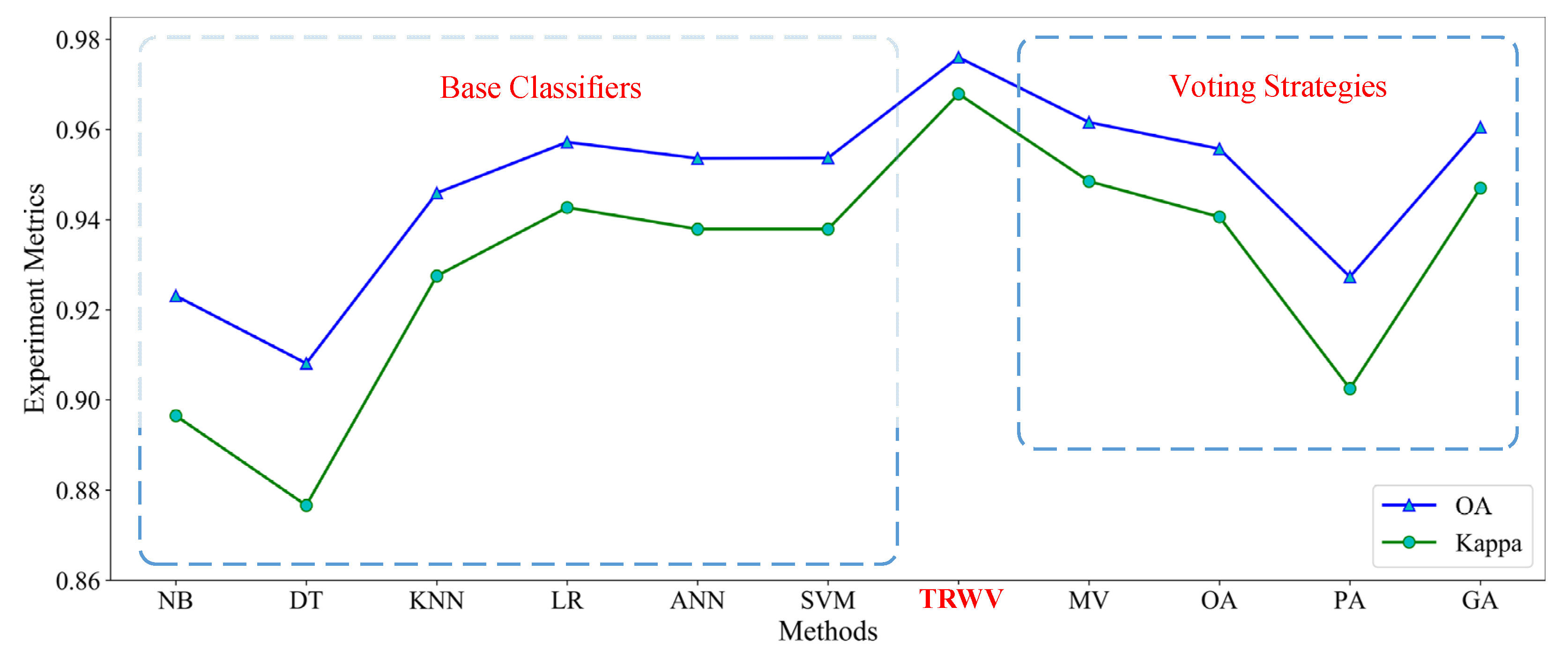
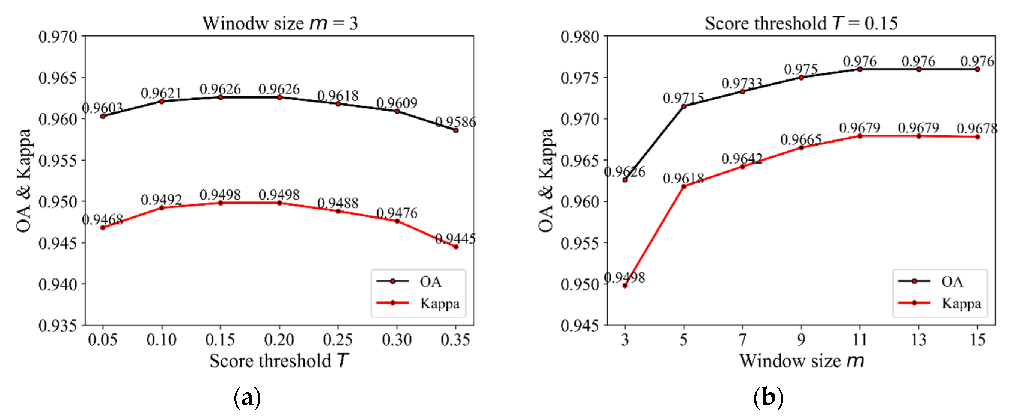
The evaluation metrics shown in Table 6 strongly demonstrate that the proposed ensemble learning method of TRWV distinctly improved the classification accuracy of the base classifiers. Meanwhile, TRWV is also superior to the ensemble classifiers with the current mainstream voting strategies in terms of the OA and kappa coefficient. To expand the application scope of the adopted two-round weight voting strategy, parametric sensitivity analysis is carried out below for two important parameters involved in the proposed method, TRWV, which are the category score threshold $T$ and the neighborhood window size $m$. By measuring the gap of the maximum and the secondary maximum of the category score, the threshold $T$ acts as the criteria for identifying each pixel as either a fuzzy or an explicit pixel. Additionally, the neighborhood window size $m$ determines the spatial scale of the local similarity, that is, how far a region defined for the explicit pixels therein can be used to rectify the central fuzzy pixel during the second weight voting stage.

As shown in Figure 11a, when $m$ is fixed at 3 and $T$ gradually increases from 0.05 to 0.15, the total classification accuracy rises from 0.9603 to the highest value of 0.9626, and the kappa coefficient increases from 0.9468 to 0.9498. However, when $T$ continuously increases from 0.15 to 0.35, the overall accuracy and kappa coefficient show a gradual downward trend. Thus, it is found that TRWV achieves the optimal classification accuracy when $T$ is taken as 0.15 in the condition of $m$ being 3. On the other hand, the effect on the classification accuracy of the neighborhood window size $m$ is still worth discussing when the threshold $T$ is fixed at 0.15. When $m$ gradually increases from 3 to 11 with a step size of 2, the overall accuracy of the classification results grows significantly from 0.9626 to the highest value of 0.9760. Meanwhile, the kappa coefficient increases from 0.9498 to 0.9678. This is mainly because a smaller window size $m$ gives rise to a narrower spatial neighborhood, thereby leading to the limited spatial context information captured during the second round of the weight voting stage. As a result, the classifier cannot effectively suppress image noise and correct mislabeled pixels. With the increase in $m$, the suppression of image noise and the final classification accuracy are both improved obviously as more spatial context information is utilized. However, it is also found that the OA and kappa coefficients remain almost unchanged after reaching the maximum value, even though the parameter $m$ continuously increases. Therefore, according to the above discussions, the category score threshold $T$ was set as 0.15 and the neighborhood window size $m$ was taken as 11 in expectation of the highest accuracy of sea ice classification.

Although several experiments have already proved that the proposed method of TRWV has an overwhelming advantage over the current mainstream voting strategies in the classification accuracy, the TRWV method is actually not dominant in terms of the computational cost. In addition to the computation cost in the first round voting stage, which is almost equivalent to that of the traditional ensemble learning method. Additional computations are still indispensable for further rectifying the fuzzy pixels based on their local similarity during the second round voting stage. Moreover, it can also be found from the accuracy evaluation results of the classification of Image II in Table 6 that the values of the OA and kappa of all classifiers are very close. There is only a very slight increase of 0.02% in the overall accuracy for TRWV compared with the base classifier of the KNN model and the ensemble classifier with the GA strategy, which both perform best in the comparison methods. Based on the previous analysis, the main reasons accounting for this can be summarized as follows:

(1)

The selection of training samples and test samples may not be objective enough. Moreover, the sea ice category is generally difficult to be interpreted from SAR images due to the influence of speckle noises, not to mention the artificial interpretation adopted in this experiment. In other words, incorrect interpretations of the pixel category are inevitable to a great extent, which thus brings about a negative impact on the performances of the classifiers.

(2)

Compared with the conventional ensemble learning methods, what makes TRWV different is that it further corrects the fuzzy pixels based on the local similarity of the neighboring explicit pixels. Therefore, if some explicit pixels in the neighborhood are incorrectly classified, the central fuzzy pixel may also be misclassified.

Through the above experiments and discussions, the effectiveness of the proposed method has been fully verified. However, the limitation of the method is that the classification performance of the ensemble learning method is mainly dependent on its base classifiers. That is, the selected base classifiers determine the classification ability of the ensemble classifier to some extent. Thus, the performance of the ensemble classifier can be further improved by introducing new base classifiers such as object-oriented methods, segmentation algorithms, or a CNN in the follow-up studies.

5. Conclusions

In this paper, a two-round weight voting strategy-based ensemble learning method was proposed for refining sea ice classification. The effectiveness of the proposed method was verified by using 18 Sentinel-1 EW dual-polarized SAR images of the Northeast Passage. In TRWV, a random forest was adopted to select the extracted polarization features and texture features to construct the preferable features of sea ice. Then, the weight corresponding to each classifier was optimized by our genetic algorithm to achieve a coarse classification result in the first round voting stage. On this basis, each pixel was divided into a fuzzy pixel or an explicit pixel by introducing a predefined score threshold. Finally, the fuzzy pixels can then be further rectified based on the local similarity of the neighboring explicit pixels in the second round voting stage, thereby yielding the final precise classification result. The main contributions of this study can be summarized as follows:

(1)

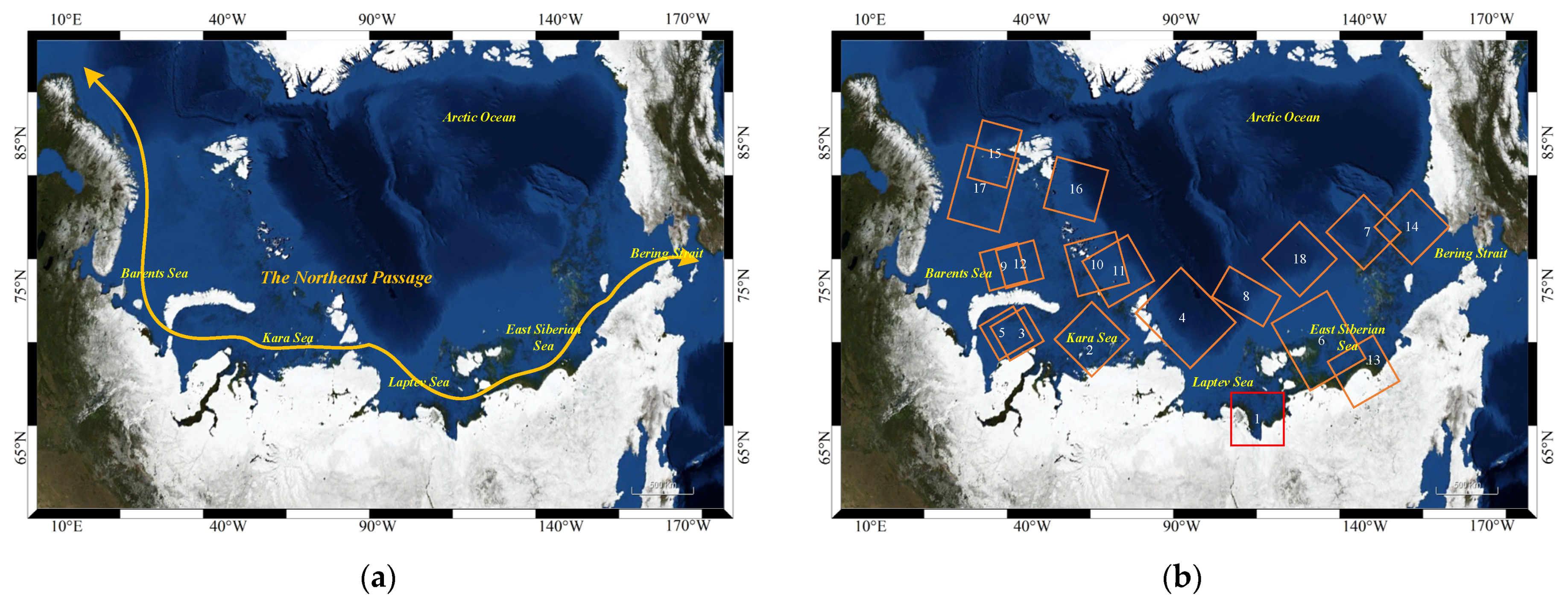
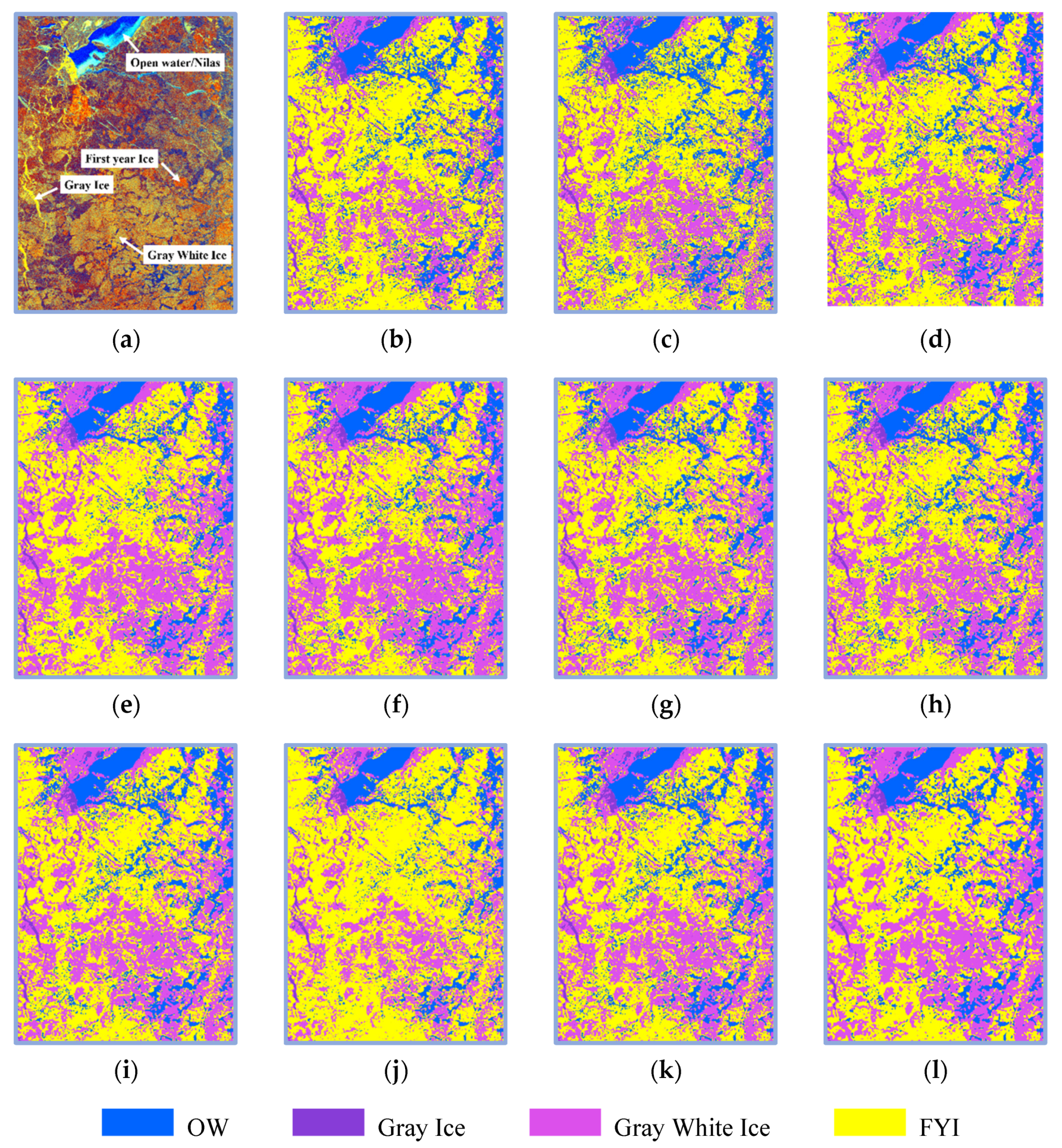
An ensemble learning method based on a two-round weight voting strategy was proposed and applied to Sentinel-1 sea ice data for the first time, achieving highly competitive classification results. The performance and effectiveness of the proposed TRWV method were investigated with Arctic sea ice scenarios from different sea areas and with different ice types. The classification results based on the multiple image scenes fully demonstrate the superiority of the proposed approach in terms of visual performance and quantitative accuracies compared with the traditional majority voting strategy and weighted voting strategy.

(2)

In this study, we evaluated the performance of six base classifiers (NB, DT, KNN, LR, ANN, and SVM) for polar sea ice classification. The experimental results show that the classification performance of logistic regression is better than the other base classifiers. By using appropriate voting strategies and integrating the advantages of different base classifiers, ensemble learning has extremely important potential for sea ice classification based on Sentinel-1 images

(3)

In this study, the idea of a two-round voting strategy was adopted for the first time to refine the classification results of the original ensemble learning, in order to improve the classification effect of sea ice. The experimental results indicate that the proposed strategy can preserve the edge contour of sea ice well, mainly because the pixels have a high correlation with their neighbors in the image spatial domain. In addition, in the process of deep mining the texture information of SAR data and calculating the similarity matrix among pixels in the neighborhood, the spatial context information is always taken into account, thus providing a guarantee for a more accurate ice classification map.

The proposed TRWV method in this paper showed a satisfactory performance of sea ice classification on Sentinel-1 images of the Northeast Passage in the winter Arctic region. However, there are still some limitations manifested in the following aspects. (1) The classification performance of the TRWV method is excessively dependent on its base classifiers. (2) Compared with the traditional voting strategies, TRWV has a higher computational cost. As a response to the above issues, the most worthwhile follow-up work of this study can be summarized as follows: (1) explore new base classifiers such as object-oriented methods, segmentation algorithms (IRGS), and CNNs; (2) adopt more efficient strategies to rectify the fuzzy pixels; and (3) evaluate the classification performance and seasonal robustness of TRWV by expanding the sea ice dataset, collecting it both in winter and summer.