Article

3D Ocean Water Wave Surface Analysis on Airborne LiDAR Bathymetric Point Clouds

1
Fujian Key Laboratory of Sensing and Computing for Smart Cities, School of Informatics, Xiamen University, Xiamen 361005, China
2
Department of Geography and Environmental Management, University of Waterloo, Waterloo, ON N2L 3G1, Canada
*
Author to whom correspondence should be addressed.
Remote Sens. 2021, 13(19), 3918; https://doi.org/10.3390/rs13193918
Submission received: 10 August 2021 / Revised: 5 September 2021 / Accepted: 23 September 2021 / Published: 30 September 2021

Abstract

:
Water wave monitoring is a vital issue for coastal research and plays a key role in geomorphological changes, erosion and sediment transportation, coastal hazards, risk assessment, and decision making. However, despite missing data and the difficulty of capturing the data of nearshore fieldwork, the analysis of water wave surface parameters is still able to be discussed. In this paper, we propose a novel approach for accurate detection and analysis of water wave surface from Airborne LiDAR Bathymetry (ALB) large-scale point clouds data. In our proposed method we combined the modified Density-Based Spatial Clustering of Applications with Noise (DBSCAN) clustering method with a connectivity constraint and a multi-level analysis of ocean water surface. We adapted for most types of wave shape anatomies in shallow waters, nearshore, and onshore of the coastal zone. We used a wavelet analysis filter to detect the water wave surface. Then, through the Fourier Transformation Approach, we estimated the parameters of wave height, wavelength, and wave orientation. The comparison between the LiDAR measure estimation technique and available buoy data was then presented. We quantified the performance of the algorithm by measuring the precision and recall for the waves identification without evaluating the degree of over-segmentation. The proposed method achieves 87% accuracy of wave identification in the shallow water of coastal zones.

Graphical Abstract

1. Introduction

Water wave surface monitoring at nearshore plays a key role in facilitating the updating of basic geographic information including geomorphological change, coastal hazards, erosion, and sediment transportation. It aids the management and maintenance of coastal areas. In addition to the function of damaging and warning system, there is a high probability of nearshore infrastructures being damaged in locations with waves. Hence, it is crucial to detect the waves before they reach coastal zones. The main challenge of ocean water wave detection is primarily due to the difficulty of acquiring high-quality data especially in the nearshore and breaking surf zone. Figure 1 shows several typical waves on nearshore shallow water.
Wave height estimation analysis has been ongoing research throughout the last century. Many researchers have studied the measurement of wave heights in coastal zones via Synthetic Aperture Radar (SAR) satellite imaging. Traditionally, a theoretical and parametric analysis was performed for the retrieval of the two-dimensional ocean waves spectra from SAR [1,2,3]. In the literature review, the C-band of Sentinel-1 SAR imagery has a wide range of products for ocean wave analysis (e.g., [4,5,6]). Parameters such as the peak of wavelengths and wave direction are calculated from C-band Scan SAR images spectra with a semi-empirical algorithm. Smit et al. [7] assimilate significant wave height from a deployed network of free-drifting satellite-connected surface weather buoys. Their assimilation strategy improves forecast accuracy with a 27% reduction in root-mean-square error in significant wave heights overall.
Furthermore, wave spectra derived from SAR images acquired by ENVISATs and SEASAT SAR were studied (e.g., [8,9,10,11]). The wave spectra inversion scheme is tailored for shallow water. The results were compared to in situ measurements by seven sensors, deployed in a field experiment. They found a reasonable agreement between in situ and SAR observations for wave heights and directions. The TanDEM-X SAR satellite also was used for ocean surface observations. There is a sensor capability within the contexts of tidal current mapping and wind-driven ocean currents as well as detection of areas with surface films [12,13].
Some other researchers employ Artificial Neural Networks (ANN) on SAR images. For instance, Ardhuin et al. [14] and Wang et al. [15] used ANN to understand the nonlinear relationship between the input SAR images parameters and output geophysical wave parameters with a data combination of altimeters and in situ buoys. Likewise, deep learning was applied to forecast time series of Significant Wave Height (SWH) [16]. They proposed a machine learning technique to create a model that relates the ocean image properties to geophysical wave parameters and predicts the sea state parameters. Their datasets comprise the SWH and wind speed data which were captured from six buoy stations in the Taiwan Strait and its adjacent waters.
Besides normal meteorological conditions, measurement of wave heights in ice zones can be implemented through SAR imaging Sentinel 1A [17,18]. They developed a nonlinear algorithm to assess the phase-resolved deterministic maps of wave-induced orbital velocities. The performance of their method for the estimation of wave parameters is expected to work best when the shortest wave components can be neglected. Despite some good results, ocean waves are not always visible in SAR images and there is a gap in detection criteria in terms of wave height, length, and direction [10]. Therefore, researchers investigated other approaches.
Microwave-radar based products were used for ocean surface observation (e.g., [19,20,21]). This research monitors the surface roughness, which is the source of the radar signal. Hwang et al. [21] studied on surface roughness and foam which are the two main contributors to ocean surface microwave thermal emission. Other research used GNSS reflectometry-based on the signal-to-noise ratio (SNR) for ocean surface observation. The distance between an antenna and the water surface is considered by analyzing the oscillation of the SNR observation [22,23,24,25]. The relationship between the sea surface roughness and the attenuation of the SNR oscillation will help to estimate the numerous significant wave height (SWH) by analyzing the SNR signal. The lack of dimension of the surface roughness spectrum and wind speed is empirically parameterized and defined as the ratio of wind friction velocity and phase speed of the surface roughness wave component [26]. Regarding numerical mathematics models, a developed model was proposed for the elevation spectrum of wind-generated ocean waves. The proposed model is a modification of the spectrum. The result of these modifications is a model simplification compared with the Pierson model [27].
Some other researchers have investigated the wave breaking analysis of the nearshore zones in both field study and laboratory experiments. In the outdoor field study, research was conducted at a tropical microtidal intermediate sandy beach to investigate the short-term swash-zone hydrodynamics and morphodynamics under variable wave conditions. The data was obtained from a 2D Light Detection and Ranging (LiDAR) scanner for wave height calculation at the lower foreshore and swash-induced topographic changed [28]. Another outdoor field experiment used 2D LiDAR scanners deployed from the pier at Saltburn-by-the-Sea, the UK for 6 days. The scanners monitored the surface elevation of nearshore waves from the breaking point to the run-up limit of temporal and spatial to capture the time-varying free surface throughout the surf and swash zones [29]. In the indoor laboratory experiment [30], the breakpoint location and time-varying water surface wave breaking were measured by mixing LiDAR and Sonar data. They used three SICK LMS511 commercial 2D LiDAR scanners along with multibeam sonar to obtain a complete surface elevation. Bryan et al. [30] obtained a good performance on breaking point location and changing wave height with an assessment of LiDAR data.
Additionally, some other methods were done on 2D imagery data such as infrared imagery and stereo frames. In this case, Deep Convolutional Neural Networks (DCNNs) perform to estimate wave breaking types from infrared imagery at the surf zone. Then, they classify the breaker type through logistic regression on the extracted image features. Their classification accuracy reached 89% and 93% [31,32]. In other research, the development of a remote wave gauging technique performs to estimate wave height and period from the imagery of waves in the surf zone. In this study, their implementation was done on the three image-based datasets. The suggested network is trained using integration of coincident images and in situ wave measurements. They achieved RMS errors of 0.14 m and 0.41 s for height and period [33]. In particular, [34,35,36] proposed a series of procedures for coastal wave-tracking using coastal video imagery with deep neural networks. The existing methods consist of stereo frames based methods. The speed of instant wave speed in the video domain is estimated through learning the behavior of propagated waves in the surf zone.
Recently, Airborne LiDAR widely used for coastal shallow water monitoring [37,38,39]. In this regard, the impact of upstream offshore wind farms on sea wave state has been studied with systematic flights deploying an airborne laser scanner. The analysis of the spectral energy distribution represented a re-distribution of the wave energy within the downstream area with enhanced energy at smaller wavelengths. Their results clearly show the effect of upstream wind at a distance of 55 km. Moreover, the wave profiles and coastal sea topography were studied with a commercial portable 2D laser scanner deployed from a fixed-wing aircraft. It presents sea surface topography and wave profiles on low altitude surveys (<300 m). Relative observed wave heights compared with a waverider buoy located in the same area during the LiDAR survey. The results show variations of the sea surface to within approximately 10 cm. In recent research, airborne LiDAR was used to measure ocean waves. The LiDAR data captured in the German Bight and processed for significant wave height which could be used to improve Wave Analysis Model (WAM). The results showed that SWH varied between 0.4 m and 2.3 m, and data is validated against buoy measurements during direct overpasses. They have below 15% deviation with the outputs of the third-generation numerical WAM [35,40].
Except for surface detection, the internal waves in shallow water are detected under the right conditions along with a plankton layer associated with a density gradient [41,42,43]. Likewise, two-dimensional measurements of ocean wave displacement were studied via an airborne LiDAR scanning system. The active ranging by the scanning optics can obtain passive measurements of surface emissivity and process them into a binary image. These measurements can provide information on the average statistics and the spatial distribution of breaking waves  [44].
Few efforts used 3D LiDAR point clouds for ocean water wave detection and analysis. Our proposed method was done on large-scale 3D LiDAR point cloud dataset. Our method can adapt to different types of oceanic, river, and wetlands water wave shape. Figure 2 represents the flowchart of our method. The main contributions of this paper are summarized as follows:
(1)
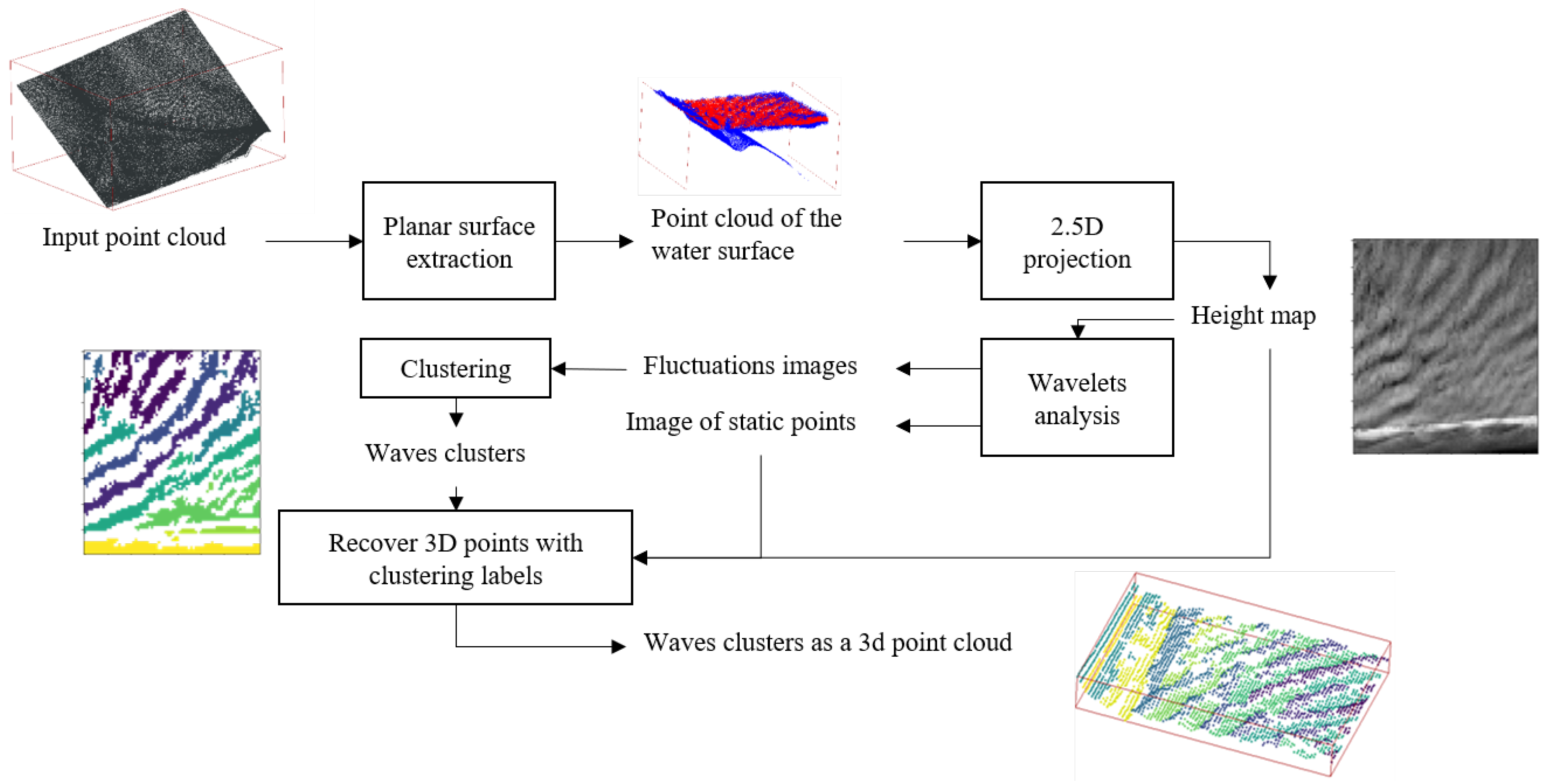
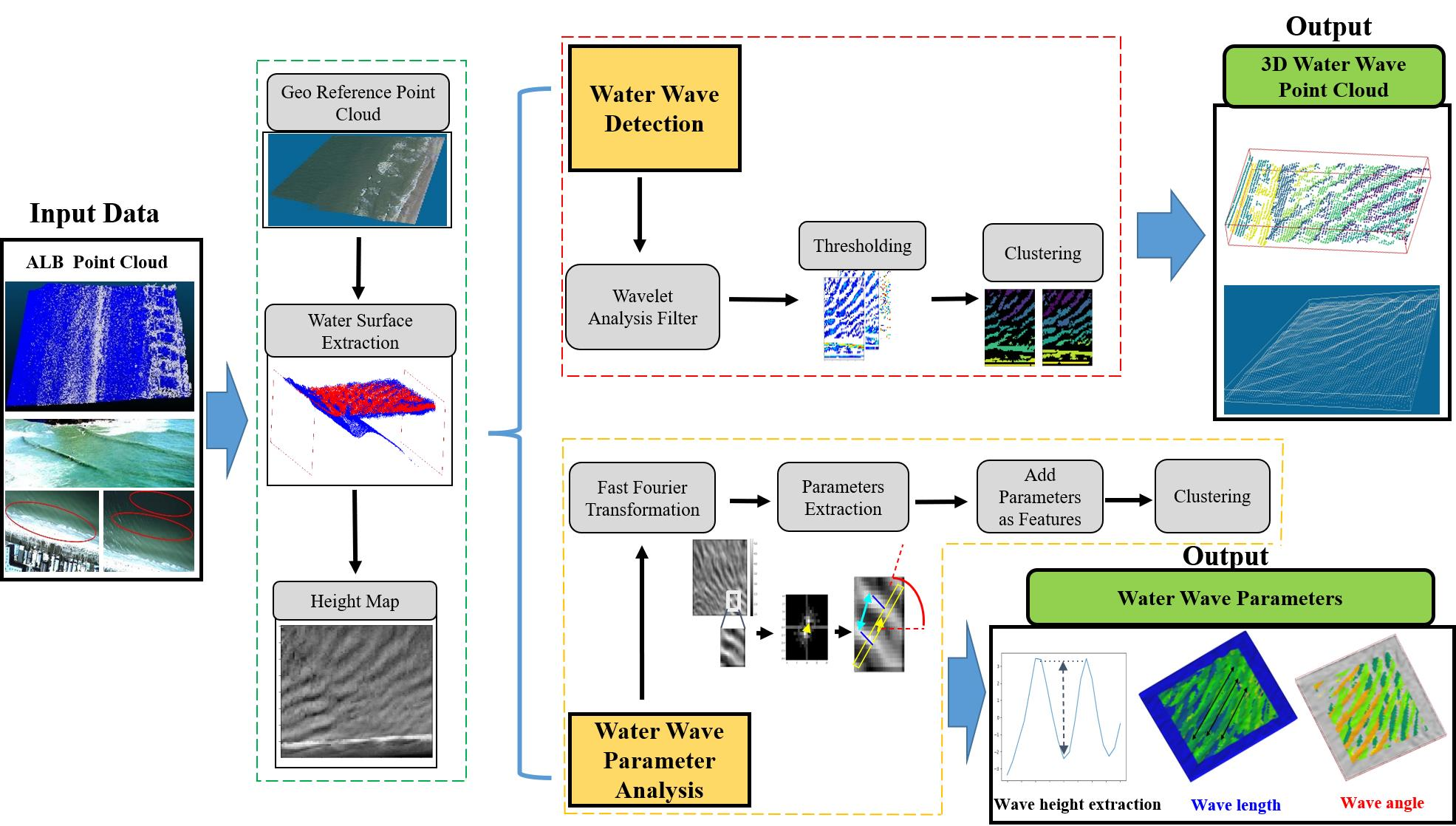
Presenting a novel water wave detection pipeline—interpretable method—which can simultaneously target different types of water waves in Airborne LiDAR Bathymetry (ALB) point clouds.
(2)
Estimation of wave parameters such as wave height, wave length, and wave orientation.
(3)
Exploring a modified Density-Based Spatial Clustering of Applications with Noise (DBSCAN) method with a connectivity constraint and a multi-level 2.5D analysis of water surface. The paper continues below.
The proposed method, experimental results, and discussion are described in Section 2, Section 3 and Section 4 respectively. Furthermore, the last section presents the conclusion and future directions.

2. Materials and Methods

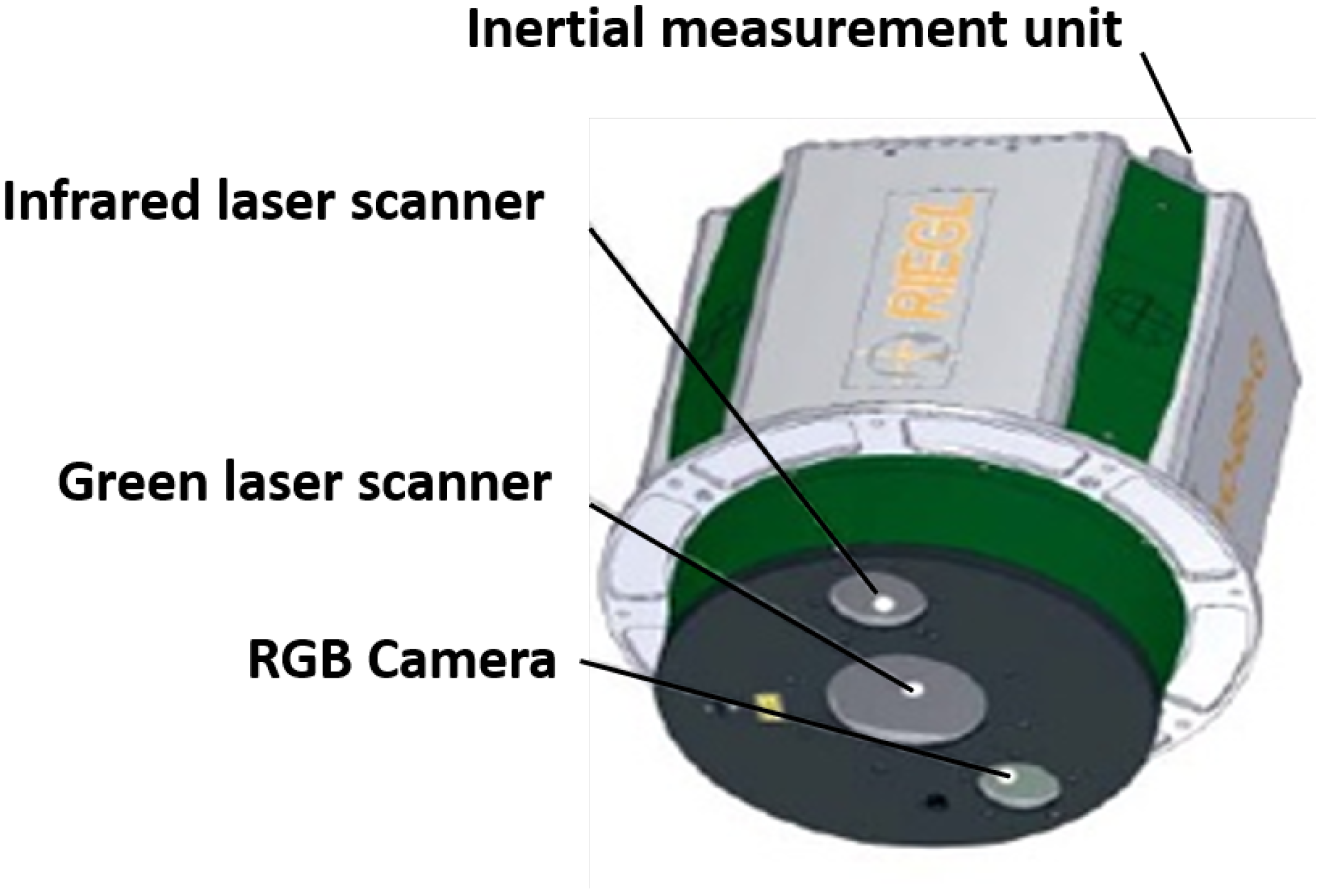
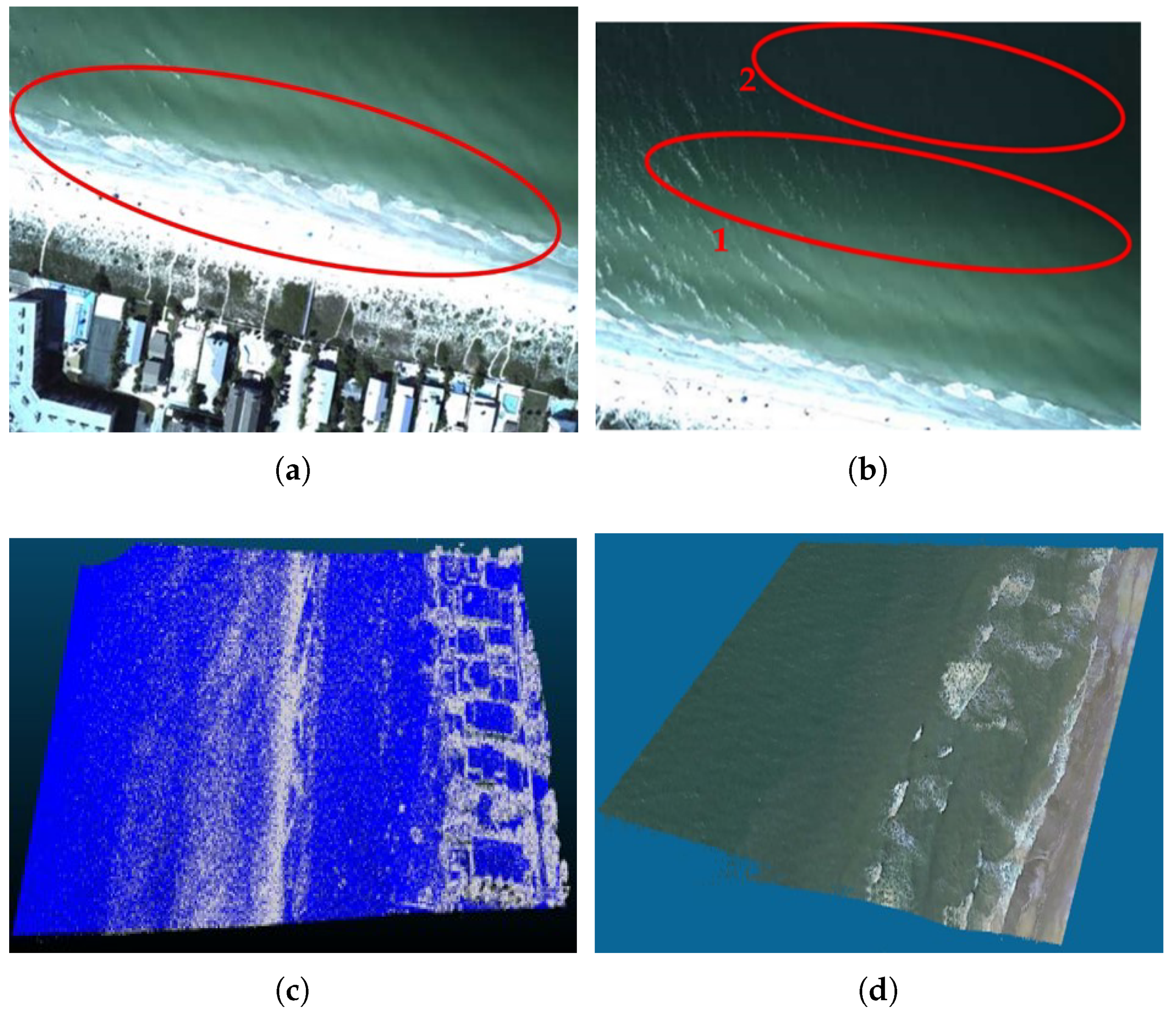
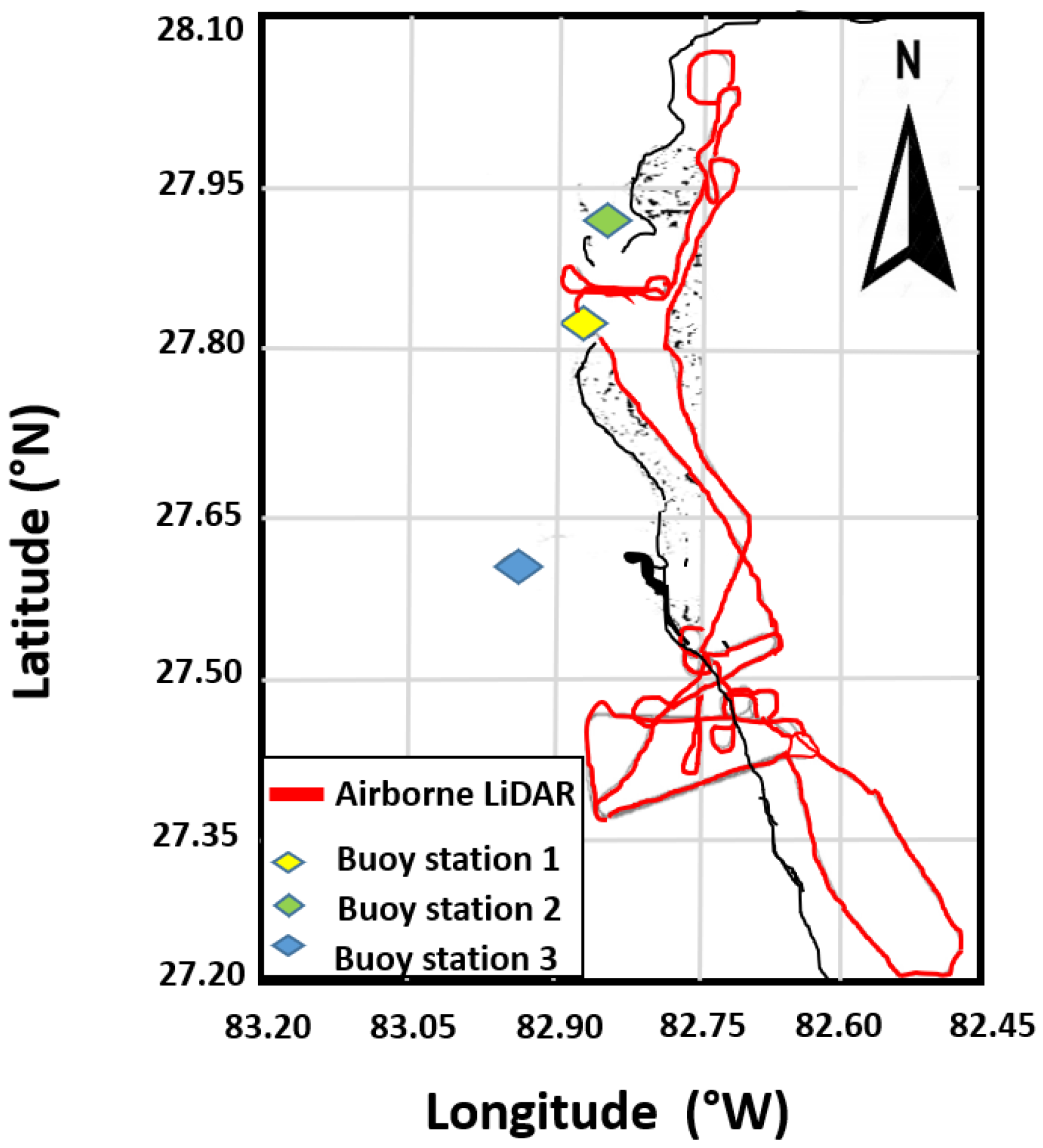
2.1. Data Description

The ALB LiDAR data in this paper are captured by a RIEGL VQ-880-G scanning system, as shown in Figure 3. The RIEGL VQ-880-G scanning system integrates laser scanners, RGB camera, and inertial navigation devices which are installed on traveling aircraft to capture accurate, high density, and precise 3D point clouds. As opposed to airborne topographic LiDAR, which uses an infrared wavelength of 1064 nm, bathymetric LiDAR systems use a green wavelength of 532 nm to penetrate the water column for measuring the seafloor. The infrared laser beam pattern is linear and the green laser beam acts in a circular pattern.
The dataset recorded by 3D LiDAR sensor is mounted on a moving air-vehicle passing through various coastal-urban scenes. The data was acquired in the beachside areas of Tampa Bay, Florida, United States, on 15 October 2015, during 1 flight in the afternoon (Time zone—GMT-05:00). Figure 4 shows the flight trajectory of Airborne LiDAR. The study area covers a large geospatial area (latitude 27 51 35 N, longitude 82 50 54 W), as a part of Florida beachside. The total number of ALB point clouds at shallow water are around 5 million points by 1.2 km × 1.8 km around.
The raw captured point cloud is adjusted with the National Oceanic and Atmospheric Administration (NOAA) benchmarks as ground control points. This transformation results in having geo-referencing for further calculation. Figure 5 shows the wave in deep and shallow water through an Airborne LiDAR Bathymetry (ALB) system at coastal urban zone. Likewise, it represents the original and geo-referenced bathymetry point clouds.
The proposed method combines a modified DBSCAN clustering method with a connectivity constraint and a multi-level 2.5 D analysis to detect water wave surface. Our approach is adaptive for most types of wave shape anatomies in deep and shallow waters, nearshore and onshore. Figure 6 and Figure 7 show the global and detailed pipeline of water wave detection. The input ALB point clouds are shifted onto the refined coordinates system, by selection planar surface inlier and discretization to voxel indices. The resulting voxel indices set will be used for the 2.5D projection. In detail, the description of each step of our pipeline is shown in Algorithm 1.
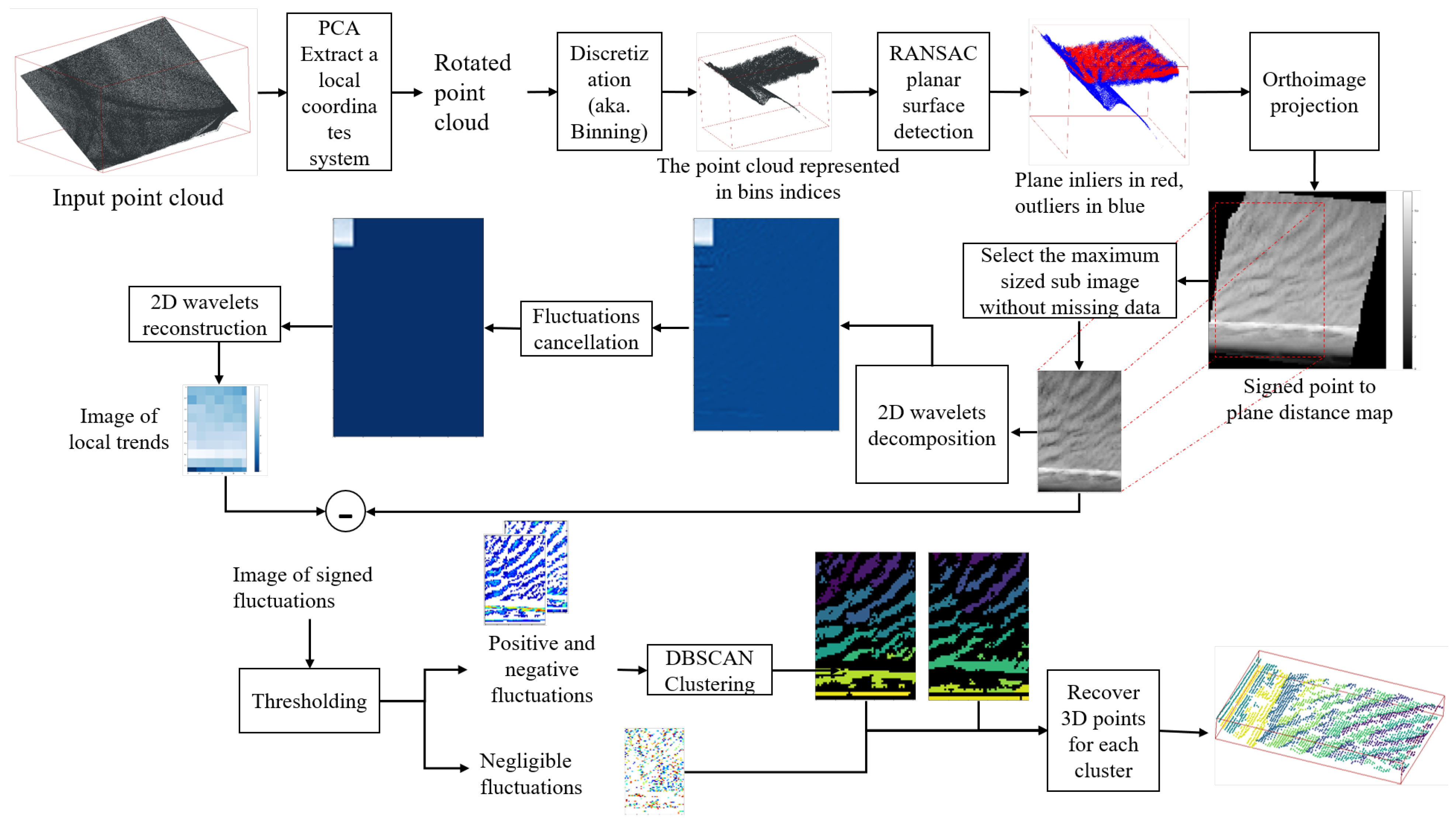
Algorithm 1 waves detection from point clouds()
Input: A point cloud P
Input: n x , n y , n z the number of range subdivisions by axis
Input: α , the standard deviation factor, used for plane inliers selection
Input: θ , the rotation angle step used for the minimum bounding box computation (typically 1 degree)
Input: The approximate size of the 2.5D height image: m × n
Input: The threshold δ s.t. any fluctuation with a magnitude lower than δ is considered stationary
Result: A copy of P with and additional field label. The label is 0 for stationary points, ≥0 for waves clusters, and −1 otherwise (e.g., underwater points)
 1: ( u 1 , u 2 , u 3 ) , I p l a n e = L R F ( P , n x , n y , n z , α , θ ) , (LRF is LocalReferenceFrame)
 2: Compute P l o c a l the projection of the point cloud onto the local reference frame
 3: P b i n s , p m i n , r = D i s c r e t i z e ( P l o c a l , n x , n y , n z )
 4: Compute the height map: I , M , m 0 , n 0 = C o m p u t e H e g h t M a p ( P b i n , m , n )
 5: Extract I c the sub-image of I without empty pixels
 6: Decompose I c in low frequency and high frequency coefficients using 2D wavelets analysis
 7: Compute I l o w the reconstruction of I using the low frequency components exclusively
 8: I d = I I l o w
 9: I s t a t i o n a r y , I + , I = S e p a r a t e F l u c t u a t i o n s ( I d , δ )
10: I + , l a b e l s = D B S C A N ( I + , 2 , c o n n e c t i v e t y D i s t a n c e ) , we use 2 as a growing radius to exclusively allow merging pixels within 1 pixel of distance the current cluster
11: I , l a b l e s = D B S C A N ( I , 2 , c o n n e t i v i t y D i s t a n c e )
12: P l a b e l s = A s s i g n L a b e l s T o P o i n t C l o u d ( P , I s t a t i o n a r y , I + , l a b e l s , I , l a b e l s )
return: P l a b e l s

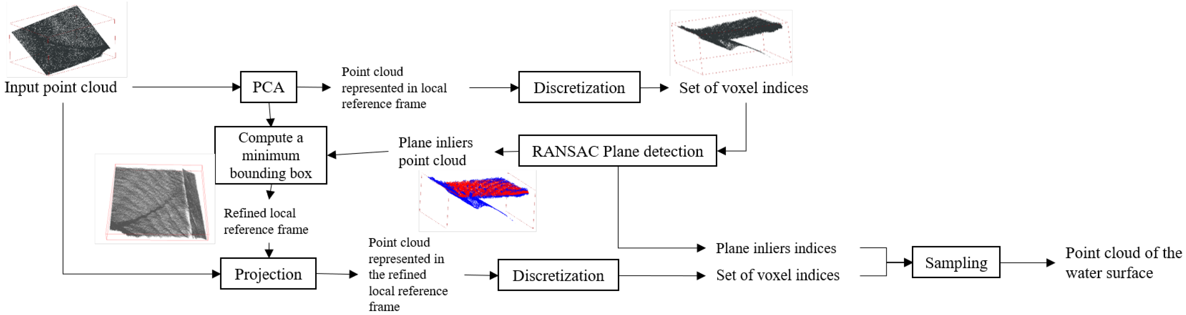
2.2. Planar Surface Extraction

We extract the water surface jointly with a coordinate system (local reference frame) in which the maximum and minimum 3D points draw a minimum volume bounding box around the water surface inliers. In this regard, first, we extract 3 principal components using Principal Component Analysis (PCA). The component with the lowest variance approximates the water surface’s normal vector since the point cloud is extended horizontally. Then, to separate the water from under-water surface, we conduct a discretization of the point cloud that acts like a standardization method. In summary, we divide the range of coordinates values in each axis to N b i n s intervals. Each interval is then indexed from 0 to N b i n s . Afterwards, the 3D space is partitioned into a set of 3D boxes, or voxels, where each box is referred by 3 bins indices. Every 3D point is then replaced by the coordinates of the box where it belongs. We then use a linear regression coupled with an outlier detector as Random Sample Consensus (RANSAC) [45] to find the planar surface with maximum inliers along with the inlier’s indices (a list of indices from 1 to N p o i n t s ). Subsequently, the inliers are then used exclusively to re-estimate the local reference frame using PCA followed by an estimation of the minimum bounding box of the planar surface. The axes of the bounding box form the refined local reference frame. We finally project the input point cloud onto the refined coordinates system, select planar surface inliers, and discretize them to voxel indices. In Figure 8, the results of voxel indices set will be used for the 2.5D projection.

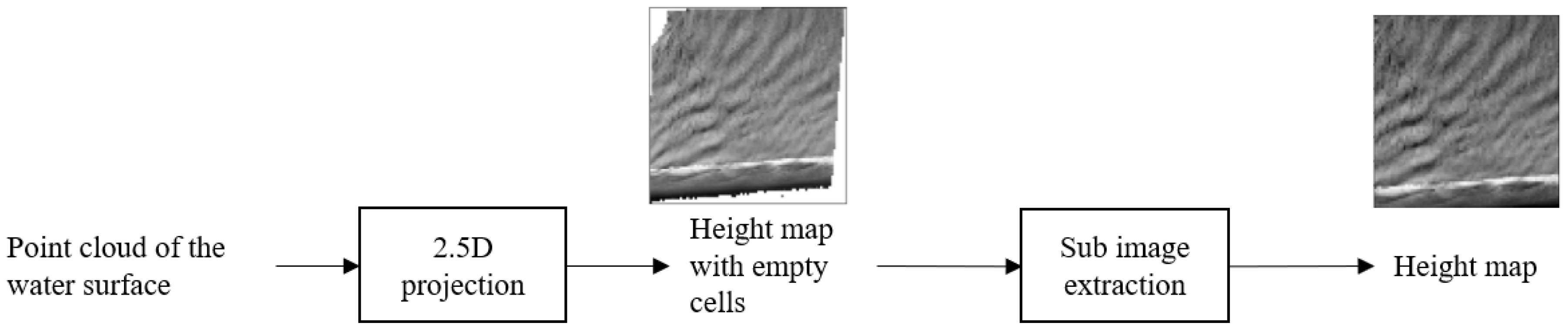
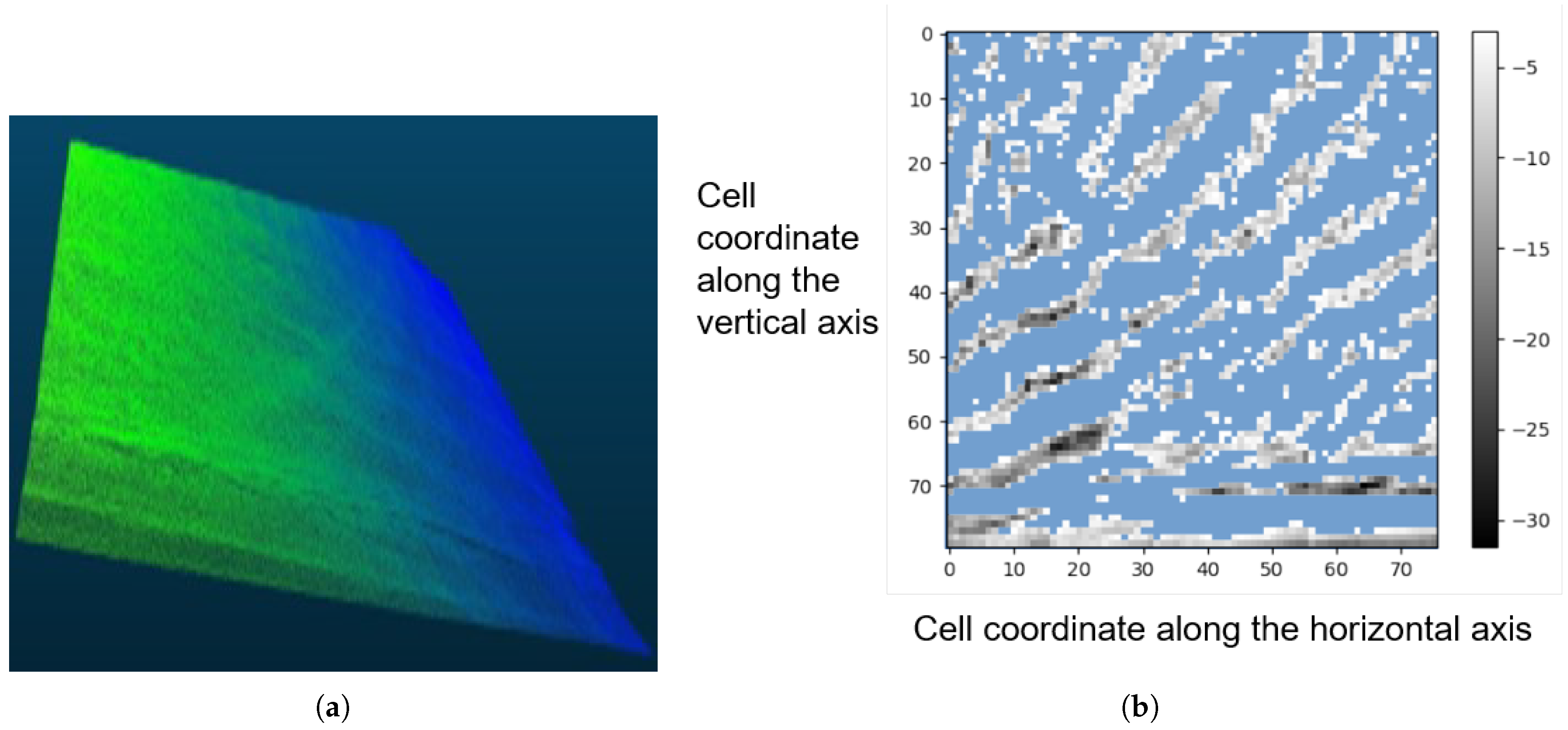
2.3. 2.5D Projection

This step aims to project the planar point cloud onto an image of signed distances to the planar surface. We first create a fictional planar grid parallel to the planar surface (or share the same normal vector of the detected plane). The 3D plane inliers are then projected onto the grid. In other terms, we assign to each 3D point the row and column indices of the grid cell where this point falls into it. Finally, we compute the average height of points in each cell and store the value in the pixel value corresponding to cell indices. Figure 9 shows the 2.5D projection. Note that we keep track of points belonging to each cell by storing their indices and cell indices in a map. This allows the recovery of 3D point clouds from pixel clusters. The grid size must be carefully chosen to minimize the number of empty cells while keeping the intrinsic details of the shape of the wave. Since the tile is not guaranteed to be square-shaped, we expect to have boundary empty cells in the projection. For this reason, we extract the maximum size sub-image without empty pixels from the original projection.

2.4. Wavelets Analysis

We use a combination of two wavelet analysis techniques, which are described as follows.

2.4.1. Wavelet Denoising

Decompose the image into a global shape (low frequency) and details (high frequency). Then cancel reconstruct again. The resulting image should look like a trend formed by the wavelet kernel [46]. Here we used a Daubechy kernel that results in locally linear trends (the neighboring pixels’ values are approximated by a linear function of pixels’ coordinates).

2.4.2. Signal Detrending Using Wavelets

The difference between the original image and the image of local trends will give an image of residuals. The residuals are chunks of the original 2D signal that separates it from a linear one. Figure 10 shows the wavelet analysis procedure.
The detrended image is then filtered by a threshold θ :
-
| I ( i , j ) | < θ gives the static pixels;
-
I ( i , j ) > θ gives concave wave parts;
-
I ( i , j ) < θ gives convex wave parts.
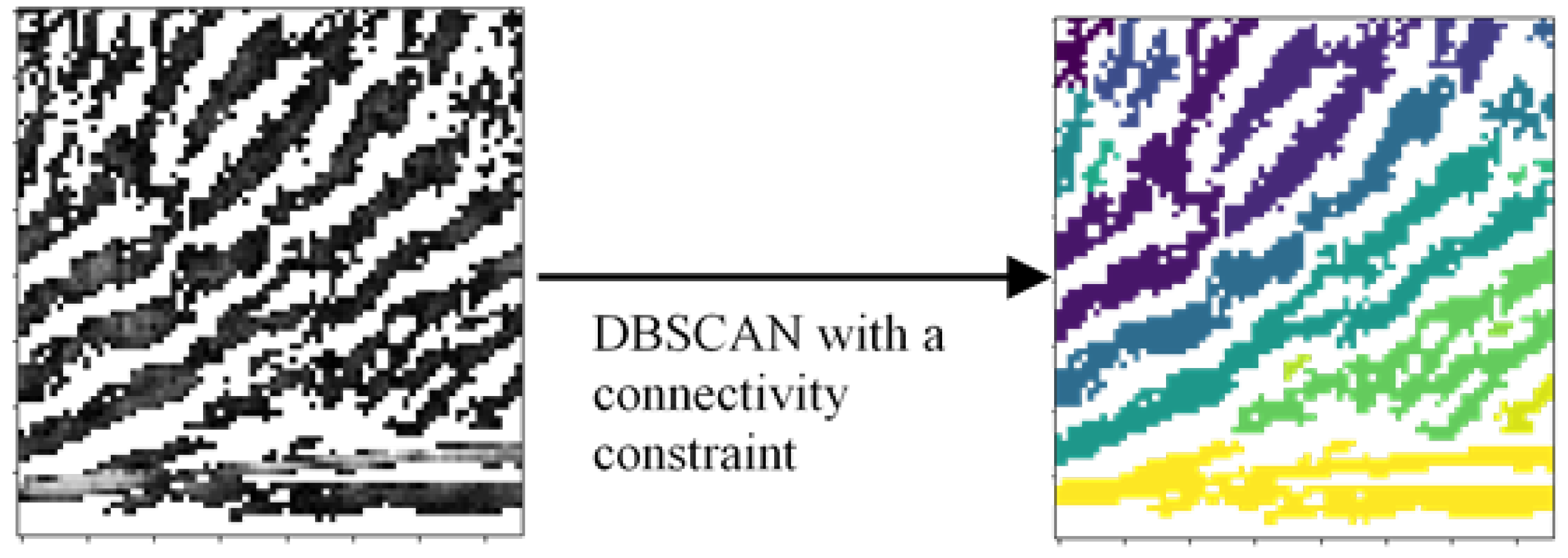
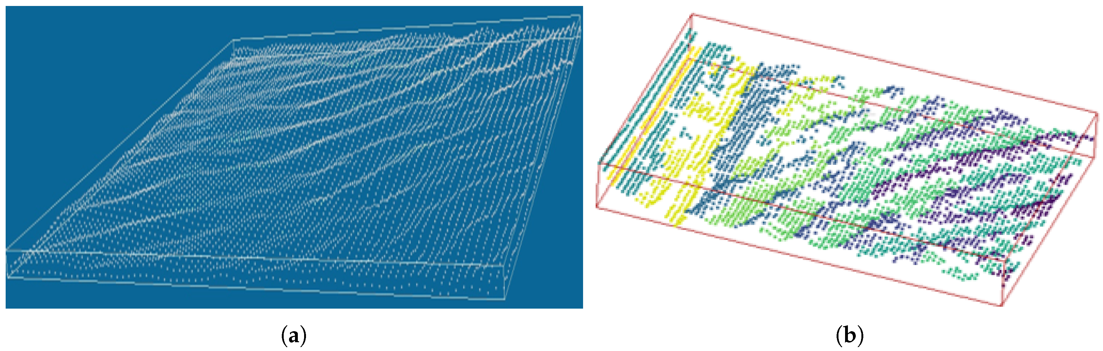
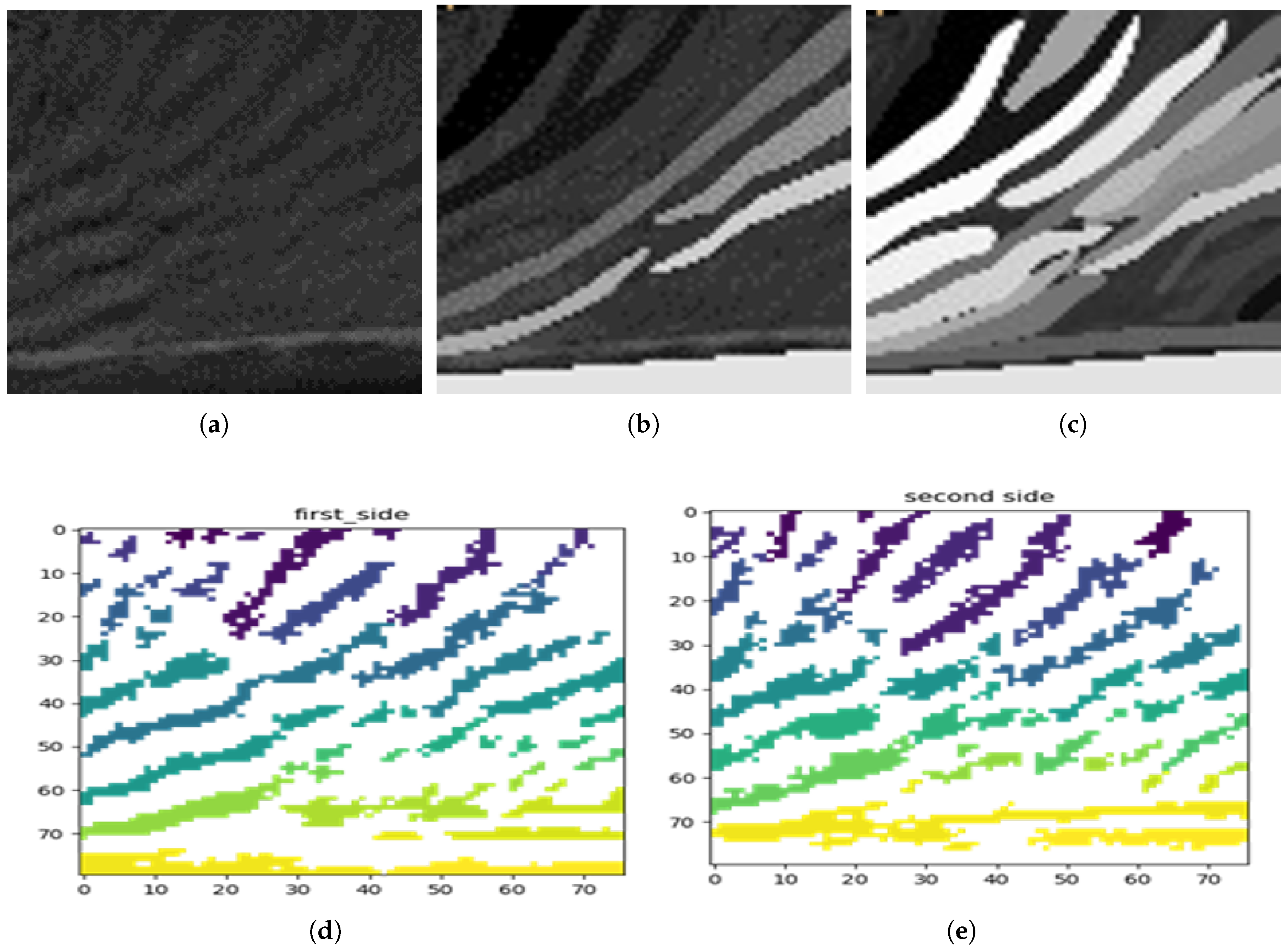
2.5. Clustering

We perform clustering of each fluctuation image using a custom distance that:
(1)
Penalizes empty pixels (connectivity constraint) by returning and infinite as the distance between an empty pixel and a valid pixel.
(2)
Returns the Euclidean distance between the pixels’ indices otherwise. Note that we do not use pixel values for the clustering as the shape of convex and concave waves are already separated by finding a suitable threshold for static points, as shown in Figure 11.

2.6. Recover 3D Points with Clustering Labels

After the clustering with DBSCAN, each wave pixel is assigned to a label and to an entry in the height map storing the indices of 3D points belonging to the pixel. To recover the clusters’ point clouds, we add a label column for the 3D points, and we proceed as follows for each image (2 fluctuation images and a static pixels’ image):
-
Initialize a label counter = 0;
-
For each label in the cluster, use the height map to recover all the indices of 3D points belonging to the cluster;
·
Replace the column label by the label counter value;
·
Increase the label counter and continue;
-
Return the point cloud with clusters’ labels.

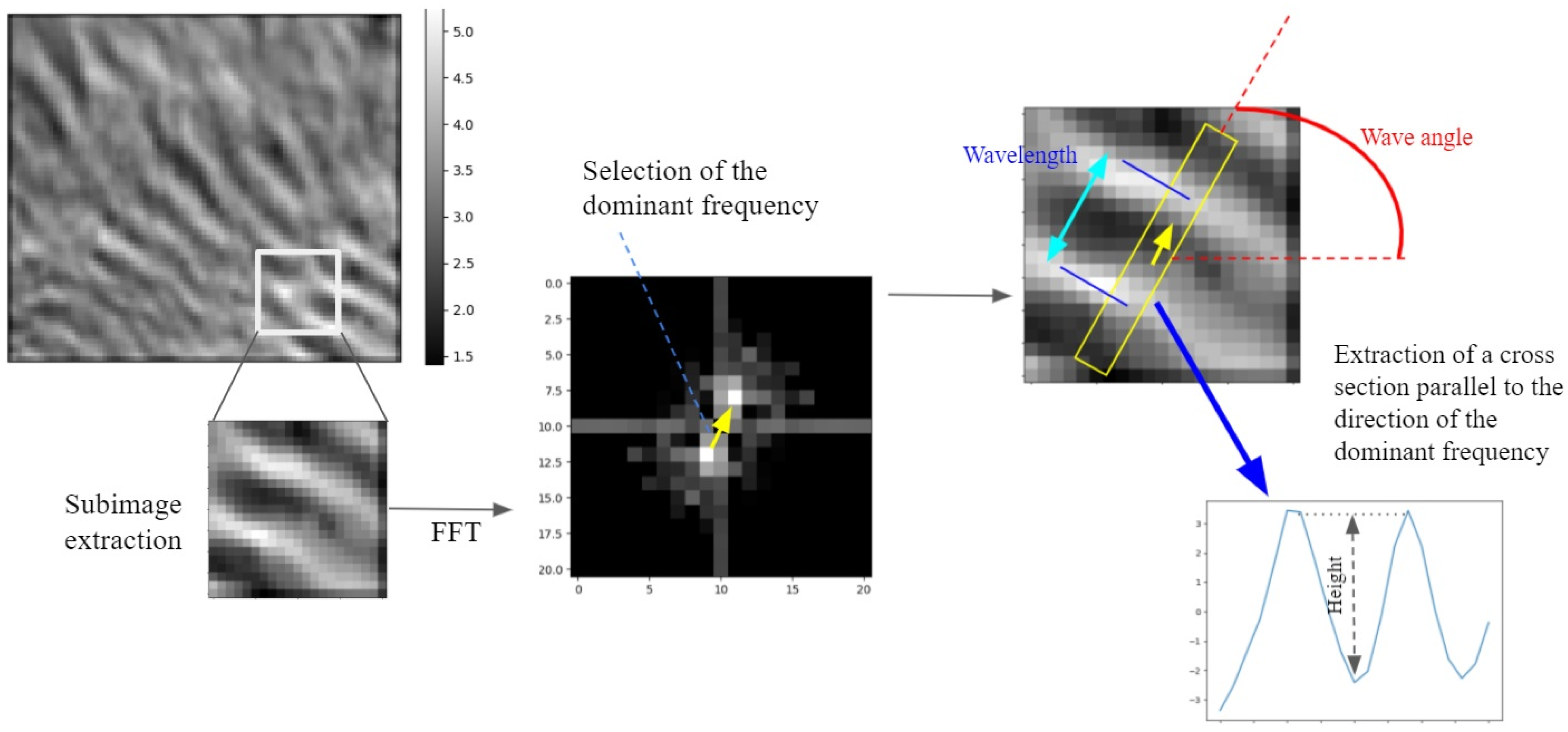
2.7. Wave Parameters Measurement

We estimate the wave parameters such as wave height measurement through Fourier Transform (FT) approach. Below Equations (1)–(3), show the sinusoidal wave Fourier equations:
F u , v = f x , y e j 2 π u x + v y d x d y ,
f x , y = F ( u , v ) e j 2 π ( u x + v y ) d u d v ,
e j 2 π ( u x + v y ) = cos 2 π u x + v y + J sin 2 π ( u x + v y )
where u and v are spatial frequencies. In addition, one can write FT pairs as f ( x , y ) = F ( u , v ) . The magnitude of the vector ( u , v ) gives a frequency, and its direction gives an orientation. The function is a sinusoid with this frequency along the direction and constant perpendicular to the direction [47]. The frequency vector is starting from the center to the white dot (max magnitude Fourier). The orientation is aligned with the wave orientation which means that the angle of the vector equals the orientation of the wave and its norm is related to wavelength. We calculate the angle by code and rotated the wave image to make it horizontal. Then we got the cross-section that travels the whole wave. Figure 12 and Figure 13 show the Fast Fourier Transfer (FFT) approach [48]. We analyzed the spectrum to extract wave parameters measurement locally and stored them in additional values. By repeating this to every patch of 21 pixels × 21 pixels around a central pixel, the result is a feature map of 3 channels. 1st layer: wave angle, 2nd layer: wavelength, and 3rd layer: wave height.

3. Results

In this section, first the water wave detection results are present. Then through the FFT approach, we show the results of wave parameters analysis.

3.1. Water Wave Detection Result

The adjustment of the parameters for the proposed algorithm is intuitive. The experiment results prove the effectiveness of the algorithm, as shown in Figure 14 and Figure 15. Figure 14a shows the top view of original point cloud at nearshore and shore and Figure 14b shows related water wave cluster detection result on the near-shore and on-shore zones. Figure 15 shows the results as 3D point cloud. We illustrate the situations in which the nearshore waves and breaking waves are placed differently: the near-shore waves are placed in the approaching shore-waves and breaking waves are placed in the breaking surf zone.
The wave cluster detection is based on wavelet analysis. The projection of the point cloud using the applied grid scheme is seen as a 2D signal and decomposed into low frequency and high frequency wavelet components. In our experiment, we used the Daubechie kernel with 3 levels of decomposition since it matches the wave patterns we want to capture. The high frequency components are then removed (overridden with zeros) and the signal is reconstructed. The reconstruction shows local trends in the point cloud projection. We then compute the residual image as the difference between the heights in the projection of the point cloud and the heights in the reconstructed projection. This difference indicates how far the signal variation is from the local trend. Typically, the residual image shows locally concave and convex crests. We then apply a threshold to remove small fluctuations and obtain a binary mask where high enough fluctuation pixels are associated with white pixels and small fluctuations are associated with black ones. The mask is finally applied to the original projection and produces Figure 14b. In the mentioned figure, the rejected fluctuations are shown with a blue mask. Selected points are shown in grayscale.

3.2. Water Waves Analysis

In our study, we analyze the wave height, wavelength, and wave direction through the ability of the Fast Fourier Transform (FFT) approach. Since FFT outputs are a spectrum, we analyze the spectrum to extract parameter measurements locally and stored them in additional values (Figure 12). We used Fast Fourier Transformation and expressed it as a linear sum of sine waves for each local point cloud (Z is a function of x and y). We picked dominant frequency assuming that locally, we should have 1 sine wave. Although it is 2D Fourier, however, pixel values store height. So we are decomposing height as a sine wave. Figure 16 shows the results of wave height, wavelength, and wave angle. In the height-map, each 3D point is associated with the wave height as a scalar field. Notice that red regions are associated with high fluctuation, whereas green and cold regions represent small ones. The blue points at the boundary are missing data due to convolution. The wave height does not show clear clusters of waves since several connected wave parts might share the same height. However, it shows regions of almost the same color. These indicate the extent of some frequencies: i.e., the extent of wave amplitude in space, or simply, the regions where the same height information can be used to describe the variation (Figure 16a). Similarly, in the wavelength map each 3D point is associated with the wavelength as a scalar field. All values seem to be relatively similar (cold range of colors), which makes sense visually from the length of the crests in the 3D render.
The wavelength information coupled with cell positions shows well defined wave parts (Figure 16b). In angle-map, each 3D point is associated with the wave angle as a scalar field as well. The selection of the points corresponding to the dominant angle shows large connected components (Figure 16c). The sea state parameters derived from ALB data provide information over a large area, including the coastal zone with similar products to the other altimetry products. In comparison, the low-resolution altimetry wave analysis and open ocean SAR wave mode products are not sufficient for local and regional applications in the complex coastal environment. Therefore, the ALB wave data would provide added value dealing with coastal processes. However, this is just one period scan time and we did an estimation of wave parameters by available data. Figure 16, Table 1, Table 2 and Table 3 show the results of wave height, wavelength, and wave angle at the nearshore zone.

3.3. Significant Wave Height Estimation

The natural definition of wave height (H) can be as the vertical distance between the highest and the lowest surface elevation in a wave shape [49]. The wave condition in a stationary record can be characterized with average wave parameters, such as the significant wave height and the significant wave period [50].
The significant wave height (SWH) is in proper correlation with the wave height as estimated ’visually’ by experienced observers. However, this is not true for the significant wave period. Significant wave height (SWH) is defined as the mean of the highest one-third of waves in the wave record:
H 1 / 3 = 1 N 3 j = 1 N / 3 H j
where j is not the sequence number in the record (i.e., the sequence in time) but the rank number of the wave, based on wave height (i.e., j = 1 is the highest wave, j = 2 is the second-highest wave, etc.). As shown in Table 1, the agreement between the estimated Significant wave height (SWH) and the measured buoy data is reasonable. To this end, regarding Table 2 and Table 3 and Equation (4), the SWH after geo-reference transformation is Hs = 0.49 m, which confirms with available buoys measurement data (station 3).

4. Discussion

In this section, in order to evaluate the performance of our method, ALB data was evaluated with available buoy data. Additionally, we calculated the assessment metrics with an annotated version of projection of the point cloud that we created.

4.1. In Situ Measurements

The sea surface is measured by directional floating buoys and the processed data is available every 30 min. In this study, three buoy stations observe the water level around the study area (station 1 ‘Clearwater Beach, FL’, station 2 ‘Fred Howard Park, FL’, and station 3 ‘Egmont Channel Entrance, FL’) along with wind speed, air temperate, significant wave height, and wind direction, Figure 4. However, station 1 and 2 did not record any wave height data during flight missions in 2015. Therefore, there is missing wave height data. The only available wave height data belongs to station 3, which was far (around 40 km) and the average wave height in station 3 is between 0.4 m and 0.7 m in 15 October 2015. This correctly confirms the algorithm output. Moreover, this new observation with ALB compensates for the missed data and shows the high capabilities of Airborne LiDAR when in situ measurement data is missed.

4.2. Satellite Observations

The launched operational altimetry satellites, e.g., Sentinel-3A and sentinel-6 were references for sea-surface height measurements until at least 2030. Satellite altimetry is radar technique-based for ocean surface height measurements with a precision of a few centimeters. However, due to the lack of available altimetry data during the study project (15 October 2015), we assess our algorithm performance with the available buoy dataset (station 3) and annotation point cloud (Section 4.3).

4.3. Quantitative Assessment Measures

We calculate the assessment metrics based on each wave of nearshore point clouds, where the precision and recall are respectively defined as Equations (5) and (6) the F1-measure is adopted to comprehensively evaluate the performance as Equation (7).
PRE = N TP N TP + N FP
REC = N TP N TP + N FN
F 1 Measure = 2 × PRE PRE + REC
N TP is the number for the correct waves points extracted; N FP is the number for the wrong points extracted; N FN is the number for the waves points that failed to extract. The quantitative results are shown in Table 4.
To evaluate the performance of our method, we created an annotated version of the projection of the point cloud as an orthoimage (Figure 17). A human labeler defines manually the most prominent waves, in other terms, the waves with the largest support. Note that in the original point cloud, waves are invisible without any processing. The water surface appears to be flat. This is one of the reasons why we chose to label the 2.5D projection. Moreover, small fluctuations are nearly invisible to the human eye. Each wave segment is associated with an index. The predictions are also associated with indices that do not necessarily match true segments. The number of segments and the ordering of predicted labels are completely independent from the annotation. As a future work, we can investigate the creation of a complete labeling framework.
Visually, we notice that the predicted wave presents small clusters that collectively overlap with most of the true clusters. We conclude that our approach provides an over-segmentation of the water surface. As a perspective, we can continue the processing by grouping segments into consistent wave parts. This requires the definition of wave consistency and the implementation of an appropriate merging policy that achieves a trade-off between over-segmentation and under-segmentation.
We quantify the performance of the algorithm by measuring the precision and recall for the wave’s identification without evaluating the degree of over-segmentation. We label all wave parts with +1 and the remaining pixels with −1. The predictions labels are changed accordingly. Note that rejected pixels (−1 as prediction) result from the small fluctuations filtering followed by DBSCAN outlier detections. The small fluctuations on the bottom right of the image are hard to identify by a human labeler. These are, however, detected by our system.
The percentage of these pixels is, hence, expected to be small relative to true −1 pixels. In our evaluation, the recall of class −1 is 52% which suggests that almost 48% of ‘not wave’ pixels were predicted as wave, such that the percentage of precision class −1, relative to all rejected pixels is 22%. Visually, an important part of these pixels is located at the “invisible” fluctuations. For the wave class, the precision is relatively important and associated with 64% recall. Similarly, the predicted wave class matches the shape of true waves except for small fluctuations. However, the support thickness of the wave segment was not predicted accurately. The missed pixels on the borders contribute to the decrease of the recall.

4.4. Complexity Analysis

The algorithm takes 2 min: 4 s ± 10 s on Ubuntu 20.04 operating system. The time was measured while having all applications and internet connections shut down. The desktop GUI and visualizations saving were deactivated. The algorithm was executed on an i7 9th generation laptop on a single processor and without use of the Graphics Processing Unit (GPU).

5. Conclusions

In this paper, we proposed an algorithm for ocean wave detection and wave analysis parameters measurement through the Airborne LiDAR Bathymetry (ALB) point cloud. Our experiments show that different types of wave shape anatomies of the ocean surface can be detected and quantified by using ALB system. By leveraging an addressing strategy, the proposed method rapidly handled large volumes of ALB point cloud toward 3D water wave detection. Our algorithm was successfully applied to the 3D ALB dataset and achieves precision of 87% for wave identification and associated with 64% recall at the shallow water of coastal zones. Visually, the predicted wave class matches with the shape of true wave except for small fluctuations. Moreover, the only available buoy station data confirms the algorithm output. The ALB wave analysis through the FFT approach provides more detailed information about spatial parameters of the wave field in the coastal zone compared with a model forecast, especially when in situ measurement data are missed. Indeed, the integration of time-varying surface data and field study data with 3D LiDAR point clouds data will improve the wave analysis accuracy measurement for real-time processing. Further research is required for additional information, such as video imagery and adding a more accurate field study detailed dataset.

Author Contributions

Conceptualization, S.R., W.L. and C.W.; methodology, S.R. and C.W.; software, S.R.; validation, S.R., W.L. and C.W.; formal analysis, J.L.; investigation, S.R. and W.L.; resources, W.L. and C.W.; data curation, C.W.; writing—original draft preparation, S.R.; writing—review and editing, W.L. and J.L.; visualization, S.R.; supervision, W.L., C.W. and J.L.; project administration, W.L. and C.W.; funding acquisition, W.L. All authors have read and agreed to the published version of the manuscript.

Funding

This work is supported by China Postdoctoral Science Foundation (No.2021M690094) and the China Scholarship Council (CSC).

Institutional Review Board Statement

Not applicable.

Informed Consent Statement

Not applicable.

Data Availability Statement

Not applicable.

Acknowledgments

We thank the reviewers for their careful reading and valuable comments, which helped us to improve the manuscript.

Conflicts of Interest

The authors declare no conflict of interest.

References

  1. Schulz-Stellenfleth, J. Ocean Wave Measurements Using Complex Synthetic Aperture Radar Data. Ph.D. Thesis, Staats-und Universitätsbibliothek Hamburg Carl von Ossietzky, Hamburg, Germany, 2003. [Google Scholar]
  2. Wang, H.; Zhu, J.; Yang, J.; Shi, C. A semiempirical algorithm for SAR wave height retrieval and its validation using Envisat ASAR wave mode data. Acta Oceanol. Sin. 2012, 31, 59–66. [Google Scholar] [CrossRef]
  3. Schulz-Stellenfleth, J.; Lehner, S.; Hoja, D. A parametric scheme for the retrieval of two-dimensional ocean wave spectra from synthetic aperture radar look cross spectra. J. Geophys. Res. Ocean. 2005, 110. [Google Scholar] [CrossRef] [Green Version]
  4. Shao, W.; Zhang, Z.; Li, X.; Li, H. Ocean wave parameters retrieval from Sentinel-1 SAR imagery. Remote Sens. 2016, 8, 707. [Google Scholar] [CrossRef] [Green Version]
  5. Ren, L.; Yang, J.; Zheng, G.; Wang, J. Significant wave height estimation using azimuth cutoff of C-band RADARSAT-2 single-polarization SAR images. Acta Oceanol. Sin. 2015, 34, 93–101. [Google Scholar] [CrossRef]
  6. Li, X.M.; Lehner, S.; Bruns, T. Ocean wave integral parameter measurements using Envisat ASAR wave mode data. IEEE Trans. Geosci. Remote Sens. 2010, 49, 155–174. [Google Scholar] [CrossRef] [Green Version]
  7. Smit, P.; Houghton, I.; Jordanova, K.; Portwood, T.; Shapiro, E.; Clark, D.; Sosa, M.; Janssen, T. Assimilation of significant wave height from distributed ocean wave sensors. Ocean Model. 2021, 159, 101738. [Google Scholar] [CrossRef]
  8. Collard, F.; Ardhuin, F.; Chapron, B. Extraction of coastal ocean wave fields from SAR images. IEEE J. Ocean. Eng. 2005, 30, 526–533. [Google Scholar] [CrossRef]
  9. Romeiser, R.; Graber, H.C.; Caruso, M.J.; Jensen, R.E.; Walker, D.T.; Cox, A.T. A new approach to ocean wave parameter estimates from C-band ScanSAR images. IEEE Trans. Geosci. Remote Sens. 2014, 53, 1320–1345. [Google Scholar] [CrossRef]
  10. Vesecky, J.F.; Stewart, R.H. The observation of ocean surface phenomena using imagery from the SEASAT synthetic aperture radar: An assessment. J. Geophys. Res. Ocean. 1982, 87, 3397–3430. [Google Scholar] [CrossRef]
  11. Bjerkaas, A.; Riedel, F. Proposed Model for the Elevation Spectrum of a Wind-Roughened Sea Surface; Technical Report; Johns Hopkins Univ Laurel Md Applied Physics Lab.: Laurel, MD, USA, 1979. [Google Scholar]
  12. Suchandt, S.; Runge, H. Ocean surface observations using the TanDEM-X satellite formation. IEEE J. Sel. Top. Appl. Earth Obs. Remote Sens. 2015, 8, 5096–5105. [Google Scholar] [CrossRef] [Green Version]
  13. Kahle, R.; Runge, H.; Ardaens, J.S.; Suchandt, S.; Romeiser, R. Formation flying for along-track interferometric oceanography—First in-flight demonstration with TanDEM-X. Acta Astronaut. 2014, 99, 130–142. [Google Scholar] [CrossRef]
  14. Ardhuin, F.; Stopa, J.; Chapron, B.; Collard, F.; Smith, M.; Thomson, J.; Doble, M.; Blomquist, B.; Persson, O.; Collins, C.O., III; et al. Measuring ocean waves in sea ice using SAR imagery: A quasi-deterministic approach evaluated with Sentinel-1 and in situ data. Remote Sens. Environ. 2017, 189, 211–222. [Google Scholar] [CrossRef] [Green Version]
  15. Wang, J.; Wang, Y.; Yang, J. Forecasting of Significant Wave Height Based on Gated Recurrent Unit Network in the Taiwan Strait and Its Adjacent Waters. Water 2021, 13, 86. [Google Scholar] [CrossRef]
  16. Stopa, J.E.; Mouche, A. Significant wave heights from S entinel-1 SAR: Validation and applications. J. Geophys. Res. Ocean. 2017, 122, 1827–1848. [Google Scholar] [CrossRef] [Green Version]
  17. Ardhuin, F.; Collard, F.; Chapron, B.; Girard-Ardhuin, F.; Guitton, G.; Mouche, A.; Stopa, J.E. Estimates of ocean wave heights and attenuation in sea ice using the SAR wave mode on Sentinel-1A. Geophys. Res. Lett. 2015, 42, 2317–2325. [Google Scholar] [CrossRef] [Green Version]
  18. Mastenbroek, C.; De Valk, C. A semiparametric algorithm to retrieve ocean wave spectra from synthetic aperture radar. J. Geophys. Res. Ocean. 2000, 105, 3497–3516. [Google Scholar] [CrossRef]
  19. Fu, L.L.; Holt, B. Internal waves in the Gulf of California: Observations from a spaceborne radar. J. Geophys. Res. Ocean. 1984, 89, 2053–2060. [Google Scholar] [CrossRef]
  20. Kropfli, R.; Ostrovski, L.; Stanton, T.; Skirta, E.; Keane, A.; Irisov, V. Relationships between strong internal waves in the coastal zone and their radar and radiometric signatures. J. Geophys. Res. Ocean. 1999, 104, 3133–3148. [Google Scholar] [CrossRef]
  21. Hwang, P.A.; Reul, N.; Meissner, T.; Yueh, S.H. Ocean surface foam and microwave emission: Dependence on frequency and incidence angle. IEEE Trans. Geosci. Remote Sens. 2019, 57, 8223–8234. [Google Scholar] [CrossRef]
  22. Roggenbuck, O.; Reinking, J.; Lambertus, T. Determination of significant wave heights using damping coefficients of attenuated GNSS SNR data from static and kinematic observations. Remote Sens. 2019, 11, 409. [Google Scholar] [CrossRef] [Green Version]
  23. Löfgren, J. Local Sea Level Observations Using Reflected GNSS Signals; Chalmers Tekniska Hogskola: Göteborg, Sweden, 2014. [Google Scholar]
  24. Roggenbuck, O.; Reinking, J. Sea surface heights retrieval from ship-based measurements assisted by GNSS signal reflections. Mar. Geod. 2019, 42, 1–24. [Google Scholar] [CrossRef]
  25. Fagundes, M.; Mendonça-Tinti, I.; Iescheck, A.; Akos, D.; Geremia-Nievinski, F. An open-source low-cost sensor for SNR-based GNSS reflectometry: Design and long-term validation towards sea-level altimetry. GPS Solut. 2021, 25, 1–11. [Google Scholar] [CrossRef]
  26. Elfouhaily, T.; Chapron, B.; Katsaros, K.; Vandemark, D. A unified directional spectrum for long and short wind-driven waves. J. Geophys. Res. Ocean. 1997, 102, 15781–15796. [Google Scholar] [CrossRef]
  27. Pierson, W.J., Jr.; Moskowitz, L. A proposed spectral form for fully developed wind seas based on the similarity theory of SA Kitaigorodskii. J. Geophys. Res. 1964, 69, 5181–5190. [Google Scholar] [CrossRef]
  28. Almeida, L.P.; Almar, R.; Blenkinsopp, C.; Senechal, N.; Bergsma, E.; Floc’h, F.; Caulet, C.; Biausque, M.; Marchesiello, P.; Grandjean, P.; et al. Lidar observations of the swash zone of a low-tide terraced tropical beach under variable wave conditions: The nha trang (vietnam) coastvar experiment. J. Mar. Sci. Eng. 2020, 8, 302. [Google Scholar] [CrossRef]
  29. Martins, K.; Blenkinsopp, C.E.; Power, H.E.; Bruder, B.; Puleo, J.A.; Bergsma, E.W. High-resolution monitoring of wave transformation in the surf zone using a LiDAR scanner array. Coast. Eng. 2017, 128, 37–43. [Google Scholar] [CrossRef]
  30. Bryan, O.; Bayle, P.M.; Blenkinsopp, C.E.; Hunter, A.J. Breaking wave imaging using lidar and sonar. IEEE J. Ocean. Eng. 2019, 45, 887–897. [Google Scholar] [CrossRef] [Green Version]
  31. Buscombe, D.; Carini, R.J. A data-driven approach to classifying wave breaking in infrared imagery. Remote Sens. 2019, 11, 859. [Google Scholar] [CrossRef] [Green Version]
  32. Stringari, C.; Harris, D.; Power, H. A novel machine learning algorithm for tracking remotely sensed waves in the surf zone. Coast. Eng. 2019, 147, 149–158. [Google Scholar] [CrossRef]
  33. Buscombe, D.; Carini, R.J.; Harrison, S.R.; Chickadel, C.C.; Warrick, J.A. Optical wave gauging using deep neural networks. Coast. Eng. 2020, 155, 103593. [Google Scholar] [CrossRef]
  34. den Bieman, J.P.; de Ridder, M.P.; van Gent, M.R. Deep learning video analysis as measurement technique in physical models. Coast. Eng. 2020, 158, 103689. [Google Scholar] [CrossRef]
  35. Bärfuss, K.; Djath, B.; Lampert, A.; Schulz-Stellenfleth, J. Airborne LiDAR Measurements of Sea Surface Properties in the German Bight. IEEE Trans. Geosci. Remote Sens. 2020, 59, 4608–4617. [Google Scholar] [CrossRef]
  36. Kim, J.; Kim, J.; Kim, T.; Huh, D.; Caires, S. Wave-tracking in the surf zone using coastal video imagery with deep neural networks. Atmosphere 2020, 11, 304. [Google Scholar] [CrossRef] [Green Version]
  37. Hwang, P.A. A note on the ocean surface roughness spectrum. J. Atmos. Ocean. Technol. 2011, 28, 436–443. [Google Scholar] [CrossRef]
  38. Vrbancich, J.; Lieff, W.; Hacker, J. Demonstration of two portable scanning LiDAR systems flown at low-altitude for investigating coastal sea surface topography. Remote Sens. 2011, 3, 1983–2001. [Google Scholar] [CrossRef] [Green Version]
  39. Bärfuss, K.; Schulz-Stellenfleth, J.; Lampert, A. The Impact of Offshore Wind Farms on Sea State Demonstrated by Airborne LiDAR Measurements. J. Mar. Sci. Eng. 2021, 9, 644. [Google Scholar] [CrossRef]
  40. Lampert, A.; Bärfuss, K.; Platis, A.; Siedersleben, S.; Djath, B.; Cañadillas, B.; Hunger, R.; Hankers, R.; Bitter, M.; Feuerle, T.; et al. In situ airborne measurements of atmospheric and sea surface parameters related to offshore wind parks in the German Bight. Earth Syst. Sci. Data 2020, 12, 935–946. [Google Scholar] [CrossRef]
  41. Churnside, J.H.; Marchbanks, R.D.; Lee, J.H.; Shaw, J.A.; Weidemann, A.; Donaghay, P.L. Airborne lidar detection and characterization of internal waves in a shallow fjord. J. Appl. Remote Sens. 2012, 6, 063611. [Google Scholar] [CrossRef] [Green Version]
  42. Lyzenga, D.R.; Bennett, J.R. Full-spectrum modeling of synthetic aperture radar internal wave signatures. J. Geophys. Res. Ocean. 1988, 93, 12345–12354. [Google Scholar] [CrossRef]
  43. Thompson, D. Calculation of radar backscatter modulations from internal waves. J. Geophys. Res. Ocean. 1988, 93, 12371–12380. [Google Scholar] [CrossRef]
  44. Hwang, P.A.; Krabill, W.B.; Wright, W.; Swift, R.N.; Walsh, E.J. Airborne scanning lidar measurement of ocean waves. Remote Sens. Environ. 2000, 73, 236–246. [Google Scholar] [CrossRef]
  45. Fischler, M.A.; Bolles, R.C. Random sample consensus: A paradigm for model fitting with applications to image analysis and automated cartography. Commun. ACM 1981, 24, 381–395. [Google Scholar] [CrossRef]
  46. Friedman, J.; Hastie, T.; Tibshirani, R. The Elements of Statistical Learning; Springer: New York, NY, USA, 2001; Volume 1. [Google Scholar]
  47. Tuckcr, M. Waves in Ocean Engineering: Measurement Analysis and Interpretation; Ellis Horwood: London, UK, 1991. [Google Scholar]
  48. Brigham, E.O. The Fast Fourier Transform and Its Applications; Prentice-Hall Inc.: Englewood Cliffs, NJ, USA, 1988. [Google Scholar]
  49. Battjes, J. A review of methods to establish the wave climate for breakwater design. Coast. Eng. 1984, 8, 141–160. [Google Scholar] [CrossRef]
  50. Holthuijsen, L.H. Waves in Oceanic and Coastal Waters; Cambridge University Press: Cambridge, UK, 2010. [Google Scholar]
Figure 1. Waves on nearshore.
Remotesensing 13 03918 g001
Figure 2. Flowchart of detection and analysis of 3D ocean water wave surface on Airborne LiDAR Bathymetric (ALB) Point Clouds.
Remotesensing 13 03918 g002
Figure 3. Airborne LIDAR Bathymetry system (RIEGL VQ-880-G).
Remotesensing 13 03918 g003
Figure 4. An Airborne LiDAR Bathymetry (ALB) measurement taken in Tampa bay, Florida, 15 October 2015, during 1 flight in the afternoon (Time zone—GMT-05:00). The maximum altitude flight is 504.617 m. The distance between buoys station 1 and 2 is 20 km and between buoys station 1 and 3 is 40 km.
Remotesensing 13 03918 g004
Figure 5. Deep-water and shallow-water waves through Airborne LiDAR Bathymetry (ALB) system. (a) Waves at surf zone (breaking form). (b): (b1) Waves at near-shore shallow water (<10 m), and (b2) deep-water (>10 m). The constant wavelength in deep-water and decreased wavelength in nearshore zone obviously can be seen. (c) Shows the top view of point clouds. Near-shore water is in gray color and deep-water is in blue color. Coastal urban buildings, trees, and beachside can be seen on the right side. Points with different reflection intensities are rendered in different colors. (d) Geo-referenced point cloud with NOAA benchmarks.
Remotesensing 13 03918 g005
Figure 6. Global pipeline of water wave detection.
Remotesensing 13 03918 g006
Figure 7. Detailed pipeline of water wave detection.
Remotesensing 13 03918 g007
Figure 8. Planar surface.
Remotesensing 13 03918 g008
Figure 9. 2.5D projection.
Remotesensing 13 03918 g009
Figure 10. Wavelet analysis procedure.
Remotesensing 13 03918 g010
Figure 11. Clustering results.
Remotesensing 13 03918 g011
Figure 12. Extraction of dominant frequency by Fast Fourier Transform (FFT) approach.
Remotesensing 13 03918 g012
Figure 13. (a) Fourier transformation of the whole point cloud. It clearly shows an almost uniform distribution of low to medium spatial frequencies. (b) An example of a local block of projected cells. (c) Fourier transform of the block. It shows one dominant spatial frequency that frequency vector starting from the center to the white dot (max magnitude Fourier). (d) Rotation of the block such that the dominant direction becomes aligned with the horizontal axis.
Remotesensing 13 03918 g013
Figure 14. (a) Top view of original (unprocessed) point cloud at study area. (b) Related water wave cluster detection results at near-shore and on-shore.
Remotesensing 13 03918 g014
Figure 15. Water waves detection results. (a,b) are 3D point cloud at shallow-water. The different colors in (b) show the waves in shore and near-shore zones.
Remotesensing 13 03918 g015
Figure 16. (a) Water wave height map from shore-line toward deep-water. Red regions are associated with high fluctuation, whereas green and cold regions represent small waves. The peak of each water wave is visible. The boundary points have no values (because of convolution). (b) Wavelength map at coastal zone. The marker shows some of the wave length. (c) Wave-angle map.
Remotesensing 13 03918 g016
Figure 17. (a) Orthoimage. (b,c) are annotated versions of the projection of the point cloud as an orthoimage. (d,e) shows the positive and negative wave detection.
Remotesensing 13 03918 g017
Table 1. The SWH values are measured by LiDAR system and buoy stations. Wind from 26 to 161 pass from coastal area.
Flight
Number
DateTimeWind Speed and Direction
WSPD (m/s)Direction (deg)
12015/10/15Evening4.4339
Flight
Number
SWH During measurement (m)
LiDARStation 3Station 2Station 1
10.490.55N/AN/A
Table 2. Quantitative Results (part 1): Wave measurement analysis results. Labels are the wave identification (which come from DBSCAN approach).
Wave
Numbers
LabelAverage Wave
Height (m)
Average Wave
Length (m)
Average Wave Angle
(Orientation) (Degree)
0−10.43210.150160.793
100.4108.088153.434
210.55110.901135
320.4339.117116.565
430.3955.450135
540.3019.117116.565
650.1695.45045
760.32211.177161.565
870.3188.088153.434
980.2258.43990
1090.3515.45045
11100.2148.43990
12110.5415.450135
13120.40011.177161.565
14130.2838.43990
15140.1894.21990
16150.2158.08826.565
17160.2694.21990
18170.37916.176153.434
19180.43810.901135
20190.3754.21990
21200.2808.43990
22210.2368.43990
23220.2735.45045
24230.24913.354146.309
25240.27911.177161.565
26250.2318.43990
27260.2455.450135
28270.4295.450135
Table 3. Quantitative Results (part 2): Wave measurement analysis results. Labels are the wave identification (which come from DBSCAN approach).
Wave
Numbers
LabelAverage Wave
Height (m)
Average Wave
Length (m)
Average Wave Angle
(Orientation) (Degree)
29280.3224.21990
30290.2358.43990
31300.2778.43990
32310.3014.21990
33320.47511.177161.565
34330.3578.43990
35340.38713.097107.489
36350.3718.43990
37360.3618.43990
38370.3508.43990
39380.6028.43990
40390.39316.176153.434
41400.36213.354146.309
42410.7648.43990
43420.3564.21990
44430.28318.726143.130
45440.3795.450135
46450.3424.21990
47460.27513.120108.434
48470.4038.43990
49480.4698.43990
50490.28714.417123.690
51500.33612.65890
52510.30012.65890
53520.79013.120108.434
54530.27518.726143.130
55540.27816.351135
56550.2578.43990
57560.3104.21990
Table 4. Quantitative results.
Waves TypePrecision (%)Recall (%)F1-Measure (%)
Negative wave (−1)0.220.520.31
Positive wave (+1)0.870.640.74
Publisher’s Note: MDPI stays neutral with regard to jurisdictional claims in published maps and institutional affiliations.

