Flood Mitigation in the Transboundary Chenab River Basin: A Basin-Wise Approach from Flood Forecasting to Management

Abstract

Rapid and reliable flood information is crucial for minimizing post-event catastrophes in the complex river basins of the world. The Chenab River basin is one of the complex river basins of the world, facing adverse hydrometeorological conditions with unpredictable hydrologic response. Resultantly, many vicinities along the river undergo destructive inundation, resulting in huge life and economic losses. In this study, Hydrologic Engineering Centre–Hydrologic Modeling System (HEC-HMS) and HEC–River Analysis System (HEC-RAS) models were used for flood forecasting and inundation modeling of the Chenab River basin. The HEC-HMS model was used for peak flow simulation of 2014 flood event using Global Precipitation Mission (GMP) Integrated Multisatellite Retrievals-Final (IMERG-F), Tropical Rainfall Measuring Mission_Real Time (TRMM_3B42RT), and Global Satellite Mapping of Precipitation_Near Real Time (GSMaP_NRT) precipitation products. The calibration and validation of the HEC-RAS model were carried out for flood events of 1992 and 2014, respectively. The comparison of observed and simulated flow at the outlet indicated that IMERG-F has good peak flow simulation results. The simulated inundation extent revealed an overall accuracy of more than 90% when compared with satellite imagery. The HEC-RAS model performed well at Manning’s n of 0.06 for the river and the floodplain. From the results, it can be concluded that remote sensing integrated with HEC-HMS and HEC-RAS models could be one of the workable solutions for flood forecasting, inundation modeling, and early warning. The concept of integrated flood management (IFM) has also been translated into practical implementation for joint Indo-Pak management for flood mitigation in the transboundary Chenab River basin.

1. Introduction

Floods are one of the most brutal catastrophes among the natural hazards [1,2,3], affect more human beings compared to other natural disasters [4,5], have the most calamitous environmental impacts [6,7], and root up enormous social–civil conflicts [8]. Hydrological hazards have encompassed a major share of fatalities and monetary damage in the history of the world [9], caused economic losses of more than 46 billion USD per year in the 21st century [10], affected more than 1.4 billion human beings, and claimed more than 220,000 lives [11]. Floods caused an economic loss of more than $1 trillion USD from 1980 to 2013 across the globe [12], deteriorated the Asian economy by $136 billion USD, and claimed an average of 22,800 lives per year [13]. History reveals that flood damages will continue to grow [14], as increased severity and frequency of floods are expected under the extremely changing climate conditions [15,16,17,18,19], which may cause severe humanitarian impacts with long-term negative waves on economic growth [20,21]. Developing countries have suffered five times more per unit of their GDPs compared with developed nations due to severe frequent floods under the prevailing climate change [22].

Unfortunately, Pakistan is a developing country that has faced a total life loss of about 12,502 in 25 major floods in its history due to extreme weather conditions. These catastrophic events caused a total economic loss of $38.171 billion USD, out of which 50% loss occurred in the past 7 years [6,23]. These huge losses are mainly due to insufficient water storage facilities, lack of budget for flood protection measures, lack of early flood-warning systems, mismanagement of disaster preparedness, and inadequate structural measures for flood mitigation [6]. The situation becomes more alarming for the Chenab River basin, where the flat topography restricts the construction of a major reservoir as a flood control structure. In the Chenab River flood of 2014, about 2.6 million people were affected, 367 people died across the country, and adjoining areas were severely affected due to the high magnitude of the flood [24]. The upcoming climate change may result in more severe and frequent floods [25], and the probable associated risks have raised public, political, and scientific awareness for sustainable flood management [26,27]. To address the destructive results of floods, a mechanism needs to be developed for flood forecasting, flood warning, and risk assessment [28,29,30,31]. The said developed mitigation strategies will eventually assist in reducing losses from unavoidable floods [32]. Therefore, flood forecasting and inundation modeling is a dire need of the time, which has always remained a big challenge for the researchers in helping administrative authorities in flood management [33,34,35,36].

Several hydrological models such as HEC-HMS, Soil Water Assessment Tool, and Water Erosion Prediction Project have been applied in river basins for hydrological modeling worldwide [37,38,39,40,41,42,43]. The HEC-HMS can simulate and forecast runoff, which primarily depends on catchment types and datasets [44,45,46,47]. Precipitation is the key parameter for hydrological modeling [48,49], and its availability and reliability are a serious issue in transboundary river basins [31,50]. Moreover, the sparse network of low-altitude meteorological observatories and the complex orography are core constraints in the estimation of in situ precipitation [51,52], while it is even more difficult to estimate precipitation in convection and snow-dominated river basins [53,54]. However, several ground and satellite-based precipitation estimates, such as the IMERG, TRMM, GSMaP_NRT, Asian Precipitation–Highly Resolved Observational Data Integration Towards Evaluation (APHRODITE), Global Precipitation Climatology Centre, and Precipitation Estimation from Remotely Sensed Information using Artificial Neural Networks, are being used for hydrological modeling by researchers worldwide [55,56,57,58,59,60,61,62].

Different hydrodynamic (1D/2D) models, such as HEC-RAS and MIKE, have been applied by different researchers for flood hazard prediction in complex river basins of the world [63,64,65,66,67,68,69]. One-dimensional flood models can simulate floods in the longitudinal direction only and cannot visualize the extent of floods over the floodplains [70], while 2D flood inundation modeling not only covers out-of-bank flows but also incorporates algorithms to account for topographic and topologic characteristics of the floodplains [71], which are the main limitations of 1D hydraulic modeling [72]. The HEC-RAS has been widely applied for hydraulic modeling and inundation mapping by different researchers across the globe [64,73,74], which requires high-resolution topographic information for demarcation of river cross sections and floodplains to delineate the flood extent, velocity, and water depth for computational nodes at different time steps [75]. The HEC-RAS-based inundation extent requires in situ flood extent information for accuracy assessment, which is difficult under flooding conditions. Therefore, the satellite-based flood extent can be helpful for this purpose.

Water body delineation, using satellite imagery and geographic information systems, provides spatiotemporal information of floods [76,77,78,79], helps to assess disastrous impacts of floods [80,81,82], and supports in water resource management [83,84]. Studies related to water body delineation have been carried out by different researchers using satellite imagery worldwide [85,86,87,88,89,90]. Water is an absorber of near-infrared (NIR) radiation, and pixels having a reflection value of less than 11% in NIR are mapped as a water body [91,92]. The high turbidity of floodwater limits the use of a single NIR threshold. However, other methods, such as the Normalized Difference Water Index (NDWI), can also be used for the purpose [85]. The NDWI, initially formulated by [93], can be used as an indicator to delineate water bodies, as it involves green and NIR bands. The NDWI takes advantage of the fact that water exhibits higher reflection in the green band and lower reflection in the NIR band [94], while vegetation and soil features exhibit high reflection in the NIR band [85], which ultimately helps to delineate water bodies using the NDWI > 0 threshold for water body delineation [95]. Landsat Enhanced Thematic Mapper Plus (ETM+) can be helpful for the delineation of water bodies with high spatial resolution [96], but clouds can introduce errors on the image acquisition date [97]. Therefore, Moderate Resolution Imaging Spectroradiometer (MODIS) daily (MOD09GA) and 8-day (MOD09A1) data can be blended with Landsat ETM+ imagery, using both NIR and NDWI methods, to overcome the errors due to clouds and spatiotemporal resolution limitations [98,99].

The Flood Early Warning System (FEWS) is a physical-based hydrodynamic model developed by the Delft Hydraulics (the Netherlands) in collaboration with National Engineering Services Pakistan and the Pakistan Meteorological Department (PMD). FEWS, consisting of SAMO (Sacramento: Rainfall-Runoff) and SOBEK (Routing) models, is being currently used in Pakistan, but malfunctioning of FEWS was also observed during the 2010 flood [100]. Efforts are being made by the Intergovernmental Hydrological Programme (IHP) of the United Nations, in collaboration with the International Centre for Water Hazard and Risk Management (ICHARM), Japan, under the umbrella of the United Nations Educational, Scientific and Cultural Organization (UNESCO) to introduce Integrated Flood Analysis System (IFAS) and Rainfall Runoff Inundation (RRI) models in Pakistan. However, all of these aforementioned efforts are in the developing phase, and there is a need to explore possible alternative techniques for flood forecasting and early warning. The main aim of the present study is to implement a basin-wise approach to develop an improved early flood warning system by integrating HEC-HMS and HEC-RAS models for flood forecasting, inundation modeling, and early warning. The present study incorporates high spatiotemporal globally gridded and satellite-based landuse, soil types, snow water equivalent (SWE), temperature, and precipitation data for flood forecasting through hydrological modeling of the transboundary Chenab River catchment using the HEC-HMS model. The study further includes finer-resolution satellite-based landuse and radiometric-terrain-corrected (RTC) information, from the Synthetic Aperture Radar (SAR), of the Chenab River floodplain for flood inundation modeling using the HEC-RAS model and satellite imagery. The study also aims to propose a way forward for flood mitigation in the transboundary Chenab River basin through implementation of IFM.

2. Materials and Methods

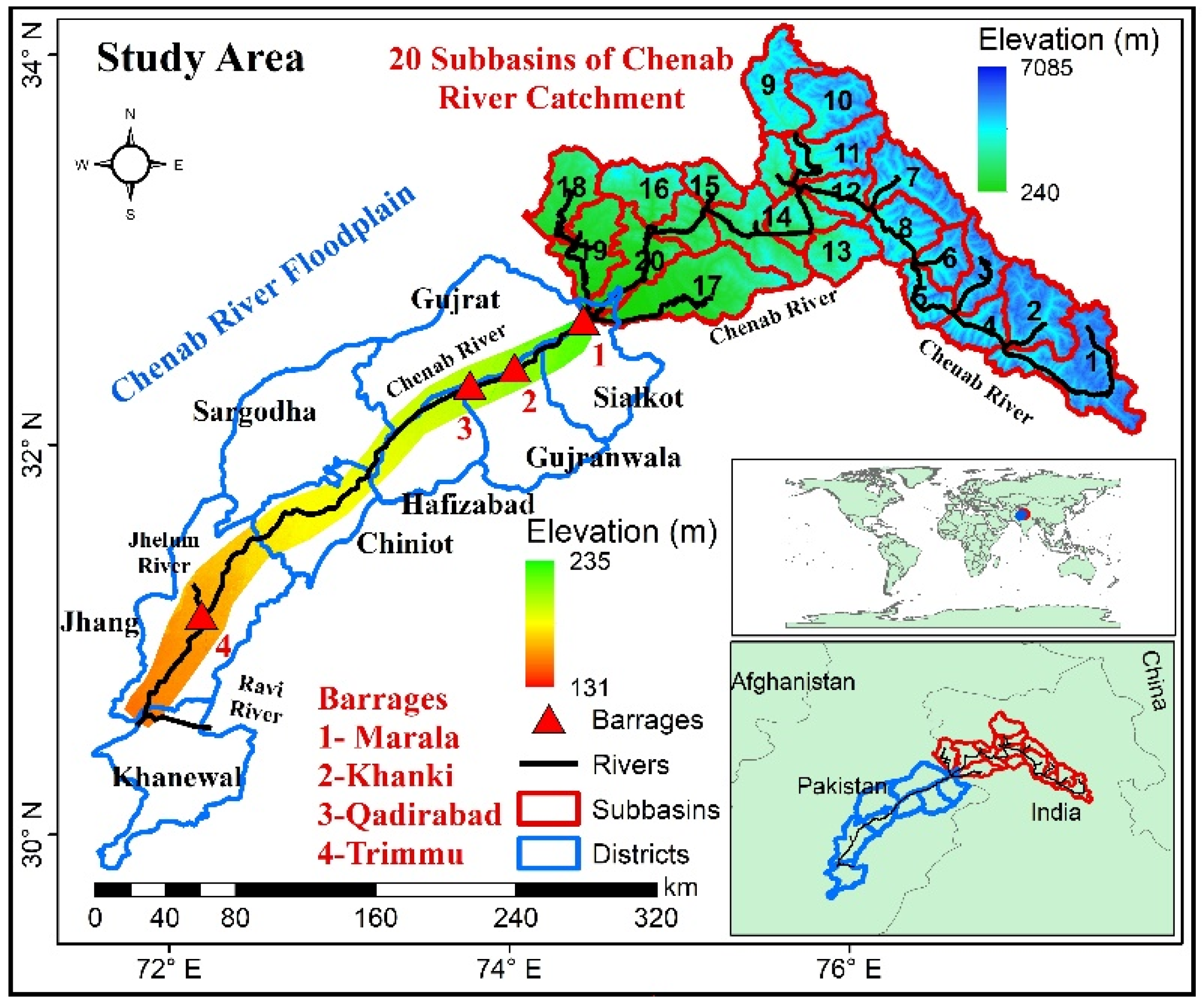
2.1. Study Area

The study area is divided in two components: (1) the upper catchment, which includes 20 subbasins contributing the flows to the Marala barrage (outlet), and (2) the lower part, which includes the river floodplain from the Marala barrage to the Chenab–Ravi Rivers’ confluence, as show in Figure 1. The geographic extent of the Chenab River catchment lies 74–77.85°E and 32–34.3°N, while elevation ranges from 240 to 7085 m. The geographic extent of the floodplain lies 71.6–74.47°E and 30.4–32.8°N, while elevation ranges from 131 to 235 m. The transboundary Chenab River basin has a total area of 67,430.34 km², of which 28,480.97 km² of catchment area is lying above the Marala barrage. The catchment area above the Marala barrage is divided among Pakistan (402 km²), Jammu and Kashmir (20,139.7 km²), and India (7939.27 km²). It clearly reflects that 27.87%, 70.71%, and 1.42% area of the catchment lies in India, Jammu and Kashmir, and Pakistan, respectively. The transboundary Chenab River in the Indian territory extends to about 230 km, and then the river enters the Jammu and Kashmir region, where it flows across a length of about 276 km. Then it enters the Marala barrage at Sialkot (Pakistan) after covering a total distance of about 506 km. The Chenab River then flows from the Marala barrage in the southwest direction to the Khanki barrage after covering a 59 km distance. The river further flows in the same direction for a downstream distance of 29 km to the Qadirabad barrage. It then proceeds toward the Trimmu barrage located at a distance of 247 km, where the Jhelum River diverts its water into the Chenab River. The last point of the study area is the confluence of the Chenab and Ravi Rivers, which is about 75 and 410 km downstream of the Trimmu and Marala barrages, respectively. The slope of the river in the upper catchment is about 25 m/km, and in the floodplain, it is about 0.4 m/km [101]. The Chenab River catchment is a snow-dominant area, and about 65% of precipitation is received in monsoon and pre-monsoon, while 26% precipitation is received in winter in the form of snow [102]. Therefore, the river receives a high magnitude of flow due to heavy precipitation in monsoon, which is augmented by the overlapped snowmelt due to the summer season. Conclusively, the peak flow from the Chenab River catchment occurs from June to September [99,103].

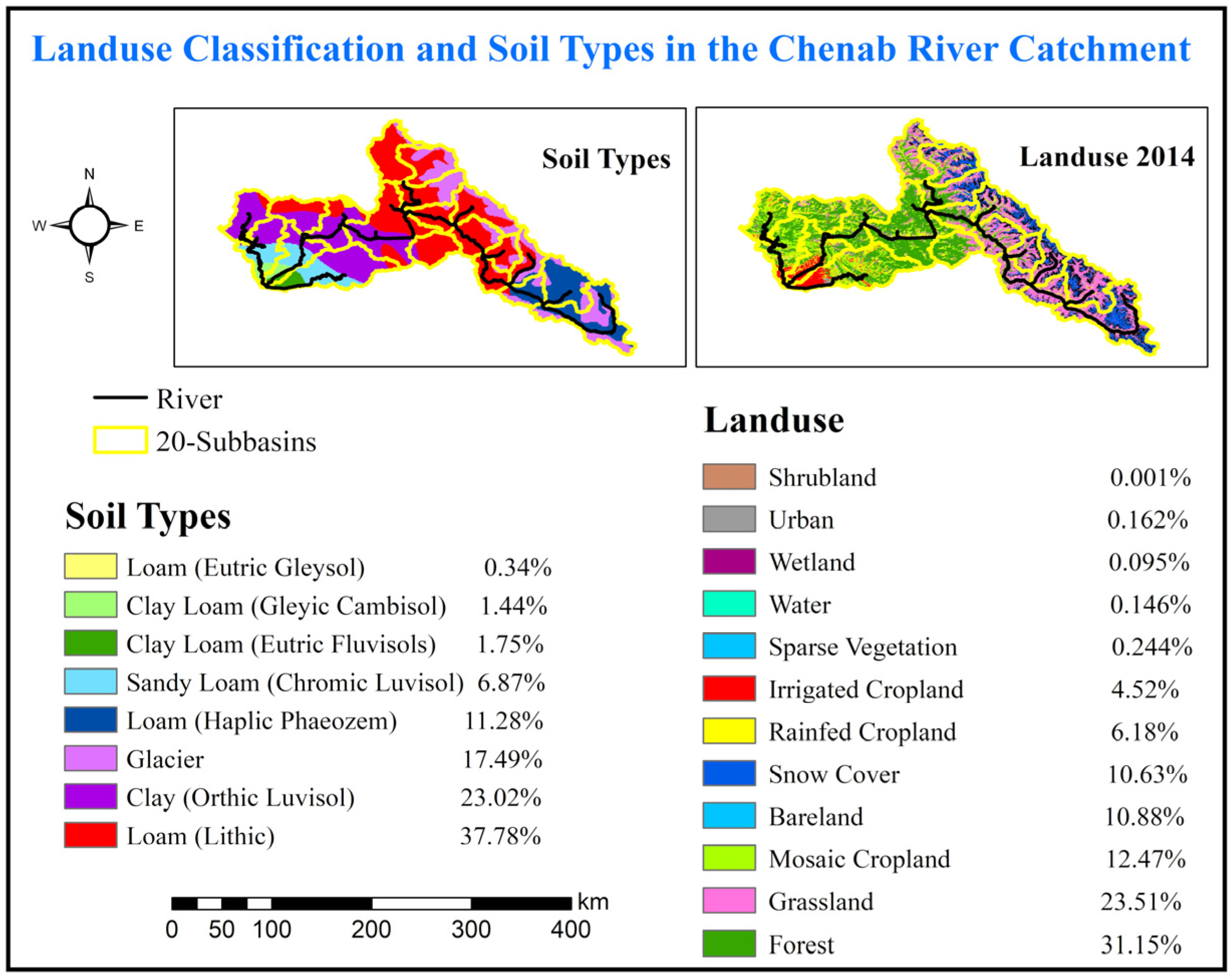
2.2. Hydrometeorological, Soil, and Landuse Datasets Used in the Study

Flood forecasting and early warning through hydrological and hydrodynamic modeling in HEC-HMS and HEC-RAS models require high spatiotemporal and reliable landuse, soil types, and all the related hydrometeorological information about the river basin [104,105,106,107,108]. Most of the Chenab River catchment is under Indian control; therefore, timely and reliable in situ hydrometeorological information is a serious issue for hydrological studies and flood forecasting. For this purpose, several satellite and global-gridded datasets were used for landuse, soil types, precipitation, temperature, and SWE information. IMERG-F for GPM Level 3 Version 6 (GPM_3IMERGDF) was used in this research, which provides daily multi-satellite precipitation at a spatial resolution of 0.1° [109]. The daily IMERG-F data depend upon the availability of half-hourly data, and the latency period for the daily data can be from 3 to 4 months. The data are processed using the Goddard Profiling Algorithm (GPROF2017) [110,111] and then gridded and intercalibrated to the GPM Combined Ku Radar-Radiometer Algorithm (CORRA) and merged into half-hourly data [112]. The daily Tropical Rainfall Measuring Mission (3B42 near Real Time (RT)) Version 7 was also used in this study at a spatial resolution of 0.25°, which is generated from 3-hourly TRMM Multi-Satellite Precipitation Analysis (TMPA) [113,114]. The TRMM_3B42RT is available after 2 months of observation due to data incorporation from multi-satellites, gauge calibration, sensor calibration, and post-processing using algorithms [115]. The GSMaP estimates have various input data sources of high spatiotemporal resolution, comprising extensive satellite information from infrared and passive microwave radiometers [116,117,118,119]. The GSMaP_NRT was also used in this research with a spatial resolution of 0.1° with a low latency period (4 h) [120,121], which is the core cause for its use in monitoring the hydrological response in the river basins. The GlobSnow SWE Level 3A product, developed by the Finnish Meteorological Institute (FMI) and Environment Canada, was used in this study at a spatial resolution of 0.25° (https://www.globsnow.info/swe/GlobSnow2_SE_SWE_Product_User_Guide_v1_r1.pdf, accessed on 21 August 2021).

Land surface temperature (LST) also plays an important role in predicting the hydrological response of the snow-dominant river catchments in the form of snowmelt [122]. For the 1992 flood event, the daily mean temperature AphroClim_V1808 (over Monsoon Asia APHRO_MA_TAVE_CLM_V1808) data was used at a spatial resolution of 0.05° (http://aphrodite.st.hirosaki-u.ac.jp/products.html, accessed on 21 August 2021). The said temperature data was developed by the APHRODITE project [123], including the Himalayas, South and Southeast Asia, and mountainous areas in the Middle East [124]. For the 2014 flood event, the global near-real-time (NRT) hourly LST data at a spatial resolution of 0.05° of geostationary satellites were incorporated in the analysis. The said NRT hourly LST data were produced after less than 3h of observation of top-of-atmosphere brightness temperatures, from the infrared spectral channels of a constellation of geostationary satellites (Meteosat Second Generation, Geostationary Operational Environmental Satellite, and Multifunction Transport Satellite/Himawari) [125].

The landuse change detection of the river catchments is a major challenge [126] and helps to understand hydrological processes and associated systems, which define the water yield from the river catchments [38,127,128,129]. Due to lack of in situ data, the global land cover map was used for 2014 for the Chenab River catchment, which was produced at a spatial resolution of 300 m by the European Space Agency (ESA) Climate Change Initiative (CCI; https://maps.elie.ucl.ac.be/CCI/viewer/, accessed on 21 August 2021) [130]. The landuse for the Chenab River floodplain was developed using Landsat 5 Thematic Mapper (TM) and Landsat 8 Operational Land Imager (OLI) for the 1992 and 2014 flood events, respectively. The supervised classification was performed using the training data (ground-truth data collected from the farming community) for each earth feature in the Chenab River floodplain for both flood events. The Normalized Difference Vegetation Index (NDVI) [131], as presented in Equation (1), was used for landuse classification at a spatial resolution of 30 m for the Chenab River floodplain, using green and NIR bands of Landsat 5 TM and Landsat 8 OLI, as presented in

Table 1. MODIS and Landsat information and thresholds of the NDWI, MNDWI 1, and MNDWI 2 used by researchers.

Satellite Products	Approach (Band)	Threshold(s)	Reference(s)
Landsat 5 TM Band 2 Green 0.52–0.60 µm Band 3 Red 0.63–0.69 µm Band 4 NIR1 0.77–0.90 µm Band 5 SWIR1 1.55–1.75 µm Band 7 SWIR2 2.08–2.35 µm	NDWI (2,4) MNDWI 1 (2,5)	0.234, 0.205 0.35, 0.45, 0.33	[162,163] [160,162,164]
Landsat 7 ETM+ Band 2 Green 0.525–0.605 µm Band 4 NIR1 0.75–0.90 µm Band 5 SWIR1 1.55–1.75 µm Band 7 SWIR2 2.09–2.35 µm	NDWI (2,4) MNDWI 1 (2,5)	0.234, 0.257 0.35, 0.45, 0.33, 0.3	[162,163] [160,162,164,165]
Landsat 8 OLI Band 3 Green 0.533–0.590 µm Band 4 Red 0.64–0.67 µm Band 5 NIR1 0.851–0.879 µm Band 6 SWIR1 1.566–1.651 µm Band 7 SWIR2 2.107–2.294 µm	NDWI (3,5) MNDWI 1 (3,6) MNDWI 2 (3,7)	0.113, 0.09 0.286, 0.33, 0.25–0.31 0.462	[157,164] [157,164,166] [157]
MODIS (MOD09GA/MOD09A1) Band 4 Green 0.545–0.565 µm Band 2 NIR1 0.841–0.876 µm Band 6 SWIR1 1.628–1.652 µm Band 7 SWIR2 2.105–2.155 µm	NDWI (4,2) MNDWI 1 (4,6)	0.0 0.44, 0.34	[167] [168,169]

.

$$\mathrm{NDVI} =\frac{\mathrm{NIR}-\mathrm{RED} }{\mathrm{NIR} +\mathrm{RED} }$$

(1)

The main purpose of the detailed landuse classification was to explore the earth features, especially the vegetation types, in the Chenab River floodplain. The Manning’s roughness coefficient (n) for each earth feature was selected from the literature [132,133] and incorporated in the numerical simulation of the HEC-RAS model.

The soil types and texture are also important, along with landuse, to understand the hydrological response of a complex river catchment [134,135]. Harmonized World Soil Database (HWSD) version 1.2 was used, which is produced at a spatial resolution of 1 km by a collaboration between the UNESCO and the Food and Agriculture Organization (FAO) with the International Institute for Applied Systems Analysis, the International Soil Reference and Information Centre (ISRIC)—World Soil Information, the Institute of Soil Science of the Chinese Academy of Sciences, and the Joint Research Centre of the European Commission (http://www.fao.org/soils-portal/data-hub/soil-maps-and-databases/harmonized-world-soil-database-v12/en/, accessed on 21 August 2021) [136].

2.3. Peak Flow Simulation Using the HEC-HMS Model

The Advanced Spaceborne Thermal Emission and Reflection Radiometer (ASTER) Digital Elevation Model (DEM) was used at a spatial resolution of 30 m for delineation of watershed, river, and river catchment using the HEC-GeoHMS model. The resultant delineated catchment and river network were imported into the HEC-HMS model for hydrological modeling. The HEC-HMS model is designed to simulate the hydrological processes of complex and dendritic river basins [137]. The HEC-HMS model can be applied to analyze the flood magnitude, flood frequency, flood warning, and spillway and reservoir planning, and can also be used for event-based and continuous hydrological modeling [46,138,139]. The soil moisture accounting (SMA) method was used for loss estimation for calibration, validation, and application periods of the HEC-HMS model, and it has been applied for event and continuous modeling worldwide [140,141,142]. The SMA method accounts for retention by canopy cover and simulates the water through soil layers to the groundwater [143]. The SMA requires the initial soil moisture condition for each subbasin at the beginning of the simulation. As a physical survey is not possible due to transboundary conflicts, the daily TMI/TRMM surface soil moisture information was retrieved from Land Parameter Retrieval Model (LPRM) Level 3 at a spatial resolution of 0.25° [144].

The snowmelt model is important for quantification of the streamflow from snow-dominant watersheds. The temperature index (TI) method was used for snowmelt runoff modeling in the HEC-HMS model due to its worldwide applications [145,146,147,148]. The TI method represents cold energy stored in the snowpack (SWE) with past conditions and all the other factors for estimation of melting for each degree above freezing temperature. The melt rate of the model is estimated by considering the present and past situations of the snowpack in the river catchment. The PX temperature (threshold temperature) differentiates snow from liquid rain, and the base temperature separates melt and non-melt periods of snow. The Soil Conservation Services Unit Hydrograph was used as the transform method, the constant monthly method was used for baseflow estimation, and the lag method was used for river routing. Automatic calibration was performed in the HEC-HMS model, which is used to minimize the objective function by fitting the best-possible agreement between the observed and the simulated flow at the gauging station [137]. The observed and simulated flows were compared at the outlet Marala barrage, as presented in Figure 1. The R², Pearson’s r, Nash and Sutcliffe efficiency (NSE), and root-mean-square error (RMSE) were used to compare the simulated flow with the observed flow, and equations are provided in Appendix A.

2.4. Numerical Simulation in the HEC-RAS Model

Two-dimensional floodplain inundation modeling requires fine-resolution topographic information about the river channel and floodplain areas [149] to get better control over the flow distribution [72,150]. For this purpose, the RTC elevation dataset (DEM) of the Phased Array type L-band SAR (PALSAR), mounted on the Advanced Land Observing Satellite-1 (ALOS), was used in the study. There were 96 cross sections, and their extraction was performed by converting the elevation model to a triangulated irregular network using the Delaunay triangulation interpolation method, which is a simple alternative of a regular raster and continuous surface with triangular facets. The extracted cross sections were corrected using Google Earth imagery to give the river a suitable and realistic shape.

The HEC-RAS v5 is a 2D numerical simulation model that be used to solve the 2D Saint Venant equation or 2D diffusive-wave equations [73,151,152]:

$$\frac{\partial \zeta }{\partial t}+\frac{\partial p}{\partial x}+\frac{\partial q}{\partial x}=0$$

(2)

$$\frac{\partial p}{\partial t}+\frac{\partial }{\partial x}\left(\frac{p^2}{h}\right)+\frac{\partial }{\partial y}\left(\frac{pq}{h}\right)=-\frac{n^{2}pg\sqrt{p^2+q^2}}{h^2}-gh\frac{\partial \zeta }{\partial x}+pf+\frac{\partial }{\rho \partial x}\left(h{\tau }_{xx}\right)+\frac{\partial }{\rho \partial y}\left(h{\tau }_{xy}\right)$$

(3)

$$\frac{\partial q}{\partial t}+\frac{\partial }{\partial y}\left(\frac{q^2}{h}\right)+\frac{\partial }{\partial x}\left(\frac{pq}{h}\right)=-\frac{n^{2}qg\sqrt{p^2+q^2}}{h^2}-gh\frac{\partial \zeta }{\partial x}+qf+\frac{\partial }{\rho \partial y}\left(h{\tau }_{yy}\right)+\frac{\partial }{\rho \partial x}\left(h{\tau }_{xy}\right)$$

(4)

where h is the depth of water (m), $g$ is the acceleration due to gravity (m s⁻²), p and q are specific flow (m² s⁻¹) in cartesian directions, n is the Manning resistance, $\zeta$ is the surface elevation (m), $\rho$ is the density of water (kg m⁻³), $f$ is the Coriolis term (s⁻¹), and ${\tau }_{xx}$, ${\tau }_{yy},$ and ${\tau }_{xy}$ are the components of effective shear stress [73]. The Coriolis term of the equation was disregarded in agreement with shallow-water assumptions and gravity flow conditions [153,154]. The inertial terms of the last 2 equations are neglected for diffusive-wave equation-based simulation. Both the Saint Venant and diffusive-wave equations were applied in the HEC-RAS model. The computing cells were created within a closed-boundary polygon, with staggered grids of rectangular cells of similar size (12.5 m × 12.5 m) and polygons of different shapes at the corners. The implicit finite volume method was applied for solving the equations, which approximates an average integral on a reference volume, and hydraulic property tables were computed before solving the equations. Elevation–hydraulic property relationships for each computational cell face and elevation–volume relationship for each cell were computed. Finally, both the equations were solved for the 2D model, and 30 iterations were preferred as compared to the coupled 1D–2D model due to limited information about overflow locations. The inflow hydrograph at the Marala barrage was applied as a boundary condition, and flow was defined in the cells covering the river width at the first cross section. The normal depth boundary conditions were applied at the borders of the model.

2.5. Satellite-Based Flood Extent Mapping

The Landsat 5 TM, Landsat 7 ETM+, Landsat 8 OLI, MOD09GA, and MOD09A1 datasets were used to map the flood extent for calibration and validation of the HEC-RAS model. The digital numbers of the Landsat images were converted to reflectance using the Fast Line-of-Sight Atmospheric Analysis of Spectral Hypercubes (FLAASH) module used for atmospheric correction [99,155,156,157]. Landsat 5 (TM), Landsat 7 ETM+, and Landsat 8 OLI have 30 m spatial resolution, while MOD09GA and MOD09A1 have 500 m spatial resolution. All the satellite datasets were then reprojected to the Universal Transverse Mercator projection and resampled at 12.5 m spatial resolution (similar to the cell size of the DEM) using the nearest-neighbor method [97,98].

By considering the higher concentration of sediments in the floodwater, different NDWI equations were applied for water body delineation for all the satellite products. The NDWI equation [93] is between the green and NIR bands:

$$\mathrm{NDWI} =\frac{\mathrm{Green}-\mathrm{NIR} }{\mathrm{Green} +\mathrm{NIR} }$$

(5)

The modified NDWI (MNDWI) can also be used as an indicator for water body delineation using green and shortwave-infrared (SWIR) bands [95,158,159], with a minimum MNDWI threshold of 0.0 [94]:

$$\mathrm{MNDWI} 1=\frac{\mathrm{Green}-\mathrm{SWIR} 1}{\mathrm{Green} +\mathrm{SWIR}1 }$$

(6)

$$\mathrm{MNDWI} 2=\frac{\mathrm{Green}-\mathrm{SWIR} 2}{\mathrm{Green} +\mathrm{SWIR}2 }$$

(7)

The bands used for calculation of the NDWI, MNDWI 1, and MNDWI 2 and their thresholds are presented in Table 1. In general, the NDWI, MNDWI 1, and MNDWI 2 range from −1 to +1, and theoretical threshold values for all the indices greater than 0 indicate water bodies in the above equations [94,155]. However, thresholds greater than 0 are not possible for all the methods [160] and all the water bodies due to sensor quality, atmospheric interference, and characteristics of water bodies, and slight adjustment of the threshold is necessary for better results [95,161]. For this purpose, all the three approaches were used with threshold values indicated in the literature by different scientists, as presented in Table 1.

The NDWI, MNDWI 1, and MNDWI 2 methods were used to delineate the blended high spatiotemporal flood extent using Landsat and MODIS products. All the three algorithms (NDWI, MNDWI 1, and MNDWI 2) were applied, owing to the high turbidity of floodwater, using thresholds recommended in the literature for flood extent delineation, and a blended flood map was developed by combining outputs of all the algorithms. The NDWI and MNDWI 1 were used for flood extent mapping using Landsat 5 (TM) for the calibration year 1992, and the blended flood extent was prepared for analysis. The NDWI, MNDWI 1, and MNDWI 2 were used to map the flood extent using Landsat 7 ETM+, Landsat 8 OLI, MOD09GA, and MOD09A1 products, and a final blended flood map was developed using outputs of all the products for the 2014 flood.

2.6. Calibration and Validation of the HEC-RAS Model

The HEC-RAS model was calibrated and validated for the flood events of 1992 and 2014, respectively, using different combinations of Manning’s n values for the main channel and floodplain. Only Landsat 5 (TM) was used for the 1992 flood event, while different satellite images were blended to produce high-resolution spatiotemporal flood extent for the 2014 flood, as presented in

Table 2. Flood events and satellite products used for water bodies delineation.

Flood Events at Barrages/Satellite Imagery	1992	2014
Marala	845,000 cusecs 10-09-1992	861464 cusecs Flood 06-09-2014
Khanki	910,500 cusecs 10-09-1992	947,000 cusecs Flood 07-09-2014
Qadirabad	948,530 cusecs 11-09-1992	904,000 cusecs Flood 07-09-2014
Trimmu	888,000 cusecs 14-09-1992	703,000 cusecs Flood 10-09-2014
Satellite Products used in the study	Landsat 5 TM 20-09-1992 29-09-1992	MOD09A1 14-09-2014 MOD09GA 09-09-2014 Landsat 7 ETM+ 09-09-2014 and 18-09-2014 Landsat 8 OLI 10-09-2014 and 17-09-2014

. Manning’s n values were selected for rivers and the floodplain using land cover data of the European Space Agency for 1992 and 2014. The roughness coefficients were further parametrized based on sensitivity analysis for the calibration year 1992. The model was calibrated and validated by comparing the inundation extent with the satellite-based inundation extent, and by comparing the simulated flow against the observed flow at barrages within the study area. Information about flow at barrages and satellite imagery used in the analysis for both the flood events are presented in Table 2. The simulated flood extent, produced by HEC-RAS against different values of Manning’s n for the river and floodplain, was compared with satellite-based inundation extent for accuracy assessment, and to fine-tune Manning’s n for the river and floodplain.

2.7. Accuracy Assessment of the HEC-RAS Model

The overall accuracy was estimated by comparing the correctly predicted flood area only (simulated cells) with the observed (satellite-based) flooded cells. It is the simplest way and provides accurate measures:

$$P_{0 }=\frac{ C_p}{n}$$

(8)

where $P_0$ is the overall accuracy, n is the total number of flooded cells observed through satellite imagery, and $C_p$ are correctly predicted (simulated) flood cells.

The performance evaluation of the model was also tested using F1 and F2 calculations recommended by [170,171]:

$$F1=\frac{A}{A+B+C}$$

(9)

$$F2=\frac{A-B}{A+B+C}$$

(10)

where $A$ is the correctly predicted flood area, which is also observed in satellite imagery; B is the predicted flood area that is not actually observed in satellite imagery; and C is the area that is not simulated as flooded area by the model but is actually observed as flooded area in the satellite imagery. F1 and F2 values ranged from 0 to +1 and −1 to +1, respectively, where higher values (near to +1) indicated a good relationship between predicted and observed flooded cells.

3. Results and Discussion

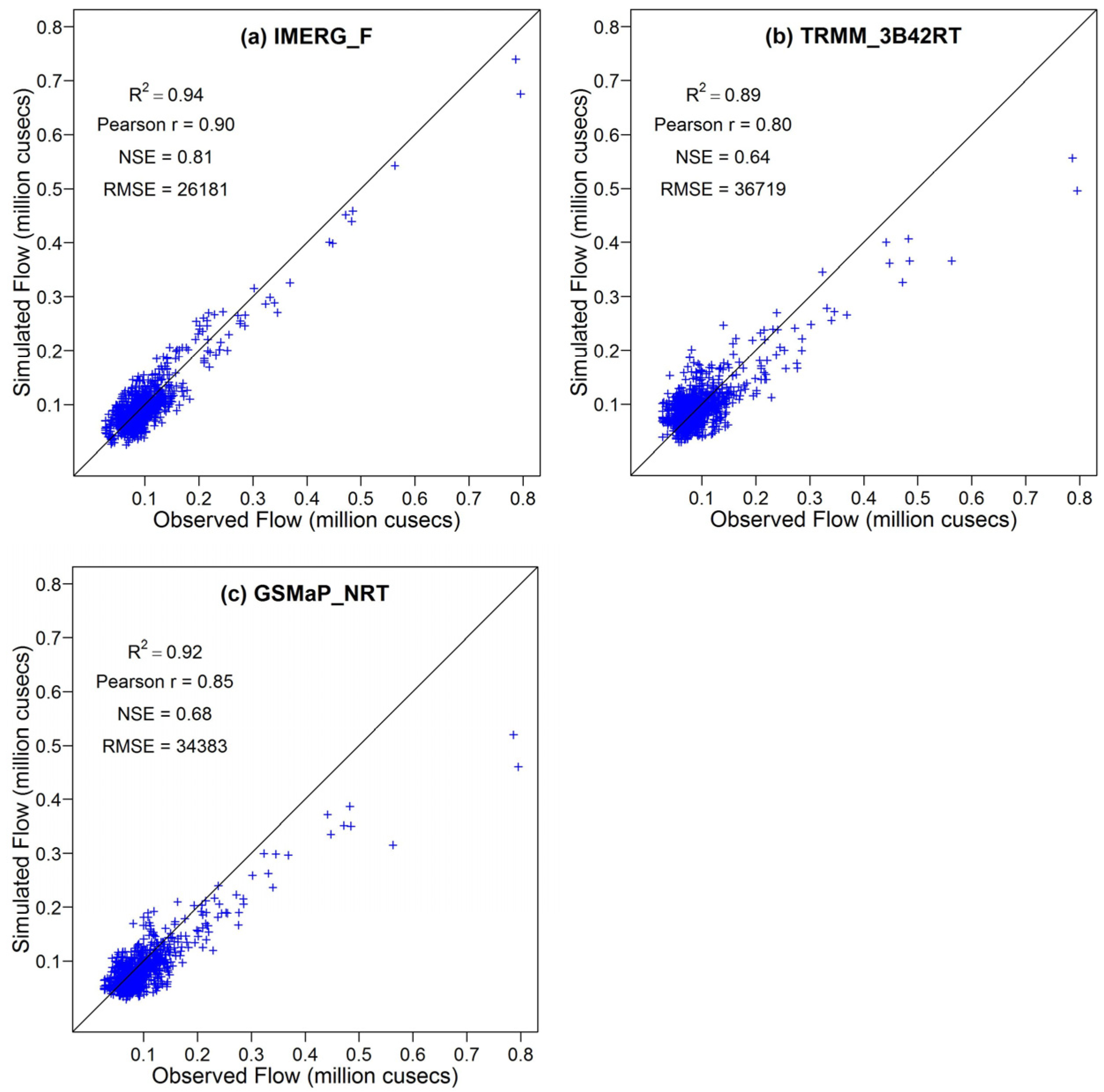
3.1. Performance Evaluation of the HEC-HMS Model

The landuse data of the ESA (2014) and HWSD are presented in Figure 2. There is a major contribution of loam and clay soil in the upper and middle catchment of the Chenab River, and a high percentage cover of a glacier is also present. The higher percentage of these mentioned classes represents major flow contribution from any high-precipitation event that can augment the surface flow significantly. The landuse map represents major landuse, such as forest, grassland, mosaic cropland, bare land and snow cover. The grassland and glacier are in the upper-to-middle part of the catchment, while forest and mosaic cropland are from the middle-to-lower parts of the catchment. The landuse of the river catchment reveals that the catchment is mostly covered by grassland and mosaic cropland and the combined effect of these two landuse features can be helpful to minimize the flood intensity. The landuse of the ESA has been successfully used by researchers for hydrological modeling of river basins [172,173].

The comparison of simulated and observed flows using all the three precipitation products for calibration, validation, and application periods are presented in Figure 3a–c. The IMERG-F-based simulated flow was in good agreement with the observed flow in validation and application periods, with higher values of R², Pearson’s r, and NSE. The IMERG-F-based simulated flow indicated slightly lower values of Pearson’s r and the NSE in the calibration period, while IMERG-F showed good performance in the peak flow simulation, which is obvious in the flood event of 2014 (Figure 3a). The TRMM_3B42RT-based simulated flow was also in reliable agreement with the observed flow in validation and application periods but with slightly lower values of R², Pearson’s r, and NSE as compared to the IMERG-F-based simulation. The TRMM_3B42RT-based simulated flow indicated a slightly fair agreement with the observed flow in the calibration period, and it did not perform well for simulation of the peak flow, which is clear in Figure 3b. The GSMaP_NRT-based simulated flow was in reliable agreement with the observed flow in calibration and application periods, with reliable values of R², Pearson’s r, and NSE, while it revealed slightly fair results in the validation period, and it did not perform well for peak flow simulation, as can be seen in Figure 3c. The scatter plots of all the simulated flows compared to the observed flow are presented in Figure 4a–c. The scatter plots covered all the calibration, validation, and application periods of the simulations. It is clear from the scatter plots that there were few deviations of points from the 1:1 line in IMERG-F-based simulation results as compared to the other simulation results. The scatter plots reveal that GSMaP_NRT-based simulation results indicate slightly lower deviations as compared to the TRMM_3B42RT-based simulation results, with slightly higher values of R², Pearson’s r, and the NSE.

A research on the same study area also revealed similar flow simulation results of IMERG-F (R² = 0.66, NSE = 0.61) and TRMM_3B42 v7 (R² = 0.64, NSE = 0.54) on the daily timescale [50]. The authors also concluded that GPM IMERG-F can be a good replacement of TRMM_3B42 v7. A hydrological study conducted by the researchers in the Beijiang River basin also revealed that IMERG-F presents satisfactory results, with a higher correlation coefficient (0.63) and NSE (0.742), with a higher probability of detection as compared to TRMM_3B42 v7, IMERG-Early, and IMERG-Late [174]. A study conducted by researchers in the Upper Huaihe River basin revealed that IMERG-F has better performance as compared to IMERG-E and IMERG-L [175]. A study conducted by researchers in Yunnan Province of China revealed that IMERG-F can capture more flood events and can be effectively used to improve the accuracy of flash flood warnings [176]. A study conducted by researchers in 300 river catchments across mainland China revealed that TRMM_3B42 has poor flow simulation performance, while IMERG-F has good results and it can be used for hydrological studies in ungauged river basins [177]. A study conducted by researchers in Myanmar watershed revealed that both IMERG-F and TRMM_3B42RT performed better in hydrological modeling, with higher NSE values of 0.84 and 0.868, respectively [178]. A study conducted by researchers in the Jhelum and Chenab River catchments revealed that GSMaP_NRT-based simulated flow underestimates peak flow events and it cannot be used for flood forecasting [179]. Reliable flow simulation performance of the GSMaP_NRT has also been observed by researchers in the Jhelum River basin, the Fuji River basin, and the sparsely gauged watershed in the Peruvian Andes [180,181,182]. From the results and discussions, it can be concluded that IMERG-F has better flow simulation performance than the other products used in the study, and IMERG-F can also be used for flood forecasting, while GSMaP_NRT and TRMM_3B42RT exhibit almost similar flow simulation results but both these products cannot be used for flood forecasting.

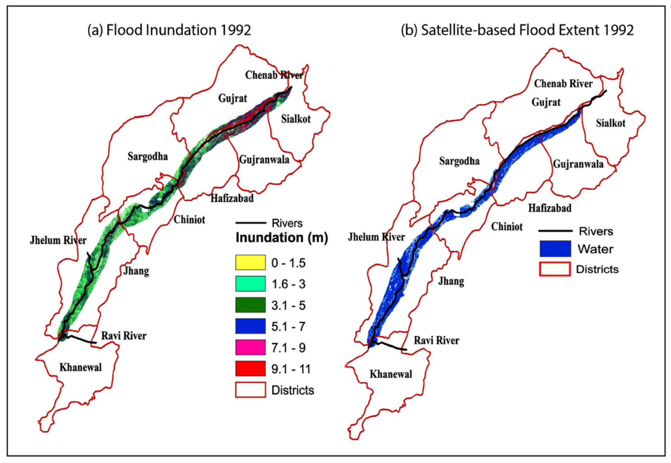
3.2. Performance Evaluation of the HEC-RAS Model

The landuse of the floodplain of the Chenab River catchment is presented in Figure 5, which was used in the HEC-RAS model for inundation modeling. The landuse of the 1992 flood event was developed using Landsat 5 TM, while the landuse of 2014 was developed using Landsat 8 OLI. The landuse plays a key role in flood propagation in the floodplain of the river basins due to variation in the roughness offered by the earth features. Manning’s runoff coefficients are also presented, along with the earth features in the floodplain of the study area, in Figure 5.

The maximum roughness coefficient is offered by forests, orchards, and sugarcane, but these classes reveal an insignificant percentage cover in the floodplain. The major contribution of landuse in the floodplain was by rice and cotton in 1992, in addition to fodders in 2014, and all these classes offered Manning’s roughness coefficient of about 0.05.

The performance assessment of the calibration event is presented in

Table 3. Calibration assessment of the model using overall accuracy, F1, and F2 for the 1992 flood.

Estimations	Floodplain n	Main Channel (River) n
		0.030	0.035	0.040	0.045	0.050	0.055	0.060
Simulated flood area (km2)	0.03	2914	3033	3122	3289	3415	3694	4112
	0.04	2976	3046	3156	3271	3468	3766	4069
	0.05	3003	3012	3144	3269	3506	3725	4125
	0.06	3056	3076	3188	3301	3539	3843	4155
Overall accuracy	0.03	75.67	76.43	80.96	83.58	84.10	86.39	89.44
	0.04	76.22	78.85	81.58	85.29	85.50	86.73	90.49
	0.05	76.51	79.14	81.78	85.52	85.81	87.28	91.43
	0.06	76.77	79.56	82.63	86.50	86.15	88.28	91.43
A	0.03	2880	2909	3081	3181	3201	3288	3404
	0.04	2901	3001	3105	3246	3254	3301	3444
	0.05	2912	3012	3112	3255	3266	3322	3480
	0.06	2922	3028	3145	3292	3279	3360	3480
B	0.03	34	124	41	108	214	406	708
	0.04	75	45	51	25	214	465	625
	0.05	91	0	32	14	240	403	645
	0.06	134	48	43	9	260	483	675
C	0.03	926	897	725	625	605	518	402
	0.04	905	805	701	560	552	505	362
	0.05	894	794	694	551	540	484	326
	0.06	884	778	661	514	527	446	326
F1	0.03	0.75	0.74	0.80	0.81	0.80	0.78	0.75
	0.04	0.75	0.78	0.81	0.85	0.81	0.77	0.78
	0.05	0.75	0.79	0.81	0.85	0.81	0.79	0.78
	0.06	0.74	0.79	0.82	0.86	0.81	0.78	0.78
F2	0.03	0.74	0.71	0.79	0.79	0.74	0.68	0.60
	0.04	0.73	0.77	0.79	0.84	0.76	0.66	0.64
	0.05	0.72	0.79	0.80	0.85	0.75	0.69	0.64
	0.06	0.71	0.77	0.81	0.86	0.74	0.67	0.63

, with an actual observed (satellite-based) flooded area of 3806 km². Manning’s n values for the channel and floodplain were selected, ranging from 0.030 to 0.060 with an interval of 0.005 and 0.01 for the channel and the floodplain, respectively. It was observed that the simulated flood extent increased by increasing the n value for the channel and floodplain. The increment in the simulated flood extent was observed more by a small increase in channel n, while the increase in the simulated flood extent was observed as low with a high increase in the n value of the floodplain. The lowest inundated area was recorded as 2914 km², and the highest inundation extent was recorded as about 4155 km². The A represents overlapped inundation of both simulated and observed data, and the maximum correctly simulated area was observed as 3480 km² at channel n of 0.060 and floodplain n of 0.04 and 0.05. The mentioned combinations of n values had a maximum overall accuracy of about 91.43% and higher values of F1 and F2, representing good and reliable results that have also been observed by researchers [170,171]. It was also clear that the values of F1 and F2 were higher at channel n of 0.04, but the overall accuracy was less at this value of n. Keeping in view all the approaches, a floodplain n of 0.05 and a channel n of 0.06 indicate the best fit for the calibration period, and the overall accuracy for all the tested combinations was more than 75%, representing reliable results.

The results of numerical simulation of 2D diffusive-wave equations were compared with the Landsat 5 (TM)-based inundation extent for the 1992 flood, as presented in Figure 6a,b. All the approaches (NDWI and MNDWI 1) were used, and outputs were blended to produce a single better inundation extent. It is clear from Figure 6a,b that simulated and observed inundated extents represented almost similar patterns in each district. However, the simulated inundation extent overestimated the observed flood extent in the Gujranwala, Hafizabad, and Chiniot districts. A flooded area was also observed on the northern side of the Ravi River due to high magnitude of the water. The area between the Chenab and the Jhelum River on the upper side of the Jhang district was inundated due to the high flood in the Jhelum River, which further augmented the flow of the Chenab River at the Trimmu barrage.

The validation of the model was performed by selecting four higher values of the main channel n against the floodplain n values, as used in the calibration, as presented in

Table 4. Validation assessment of the model using overall accuracy, F1, and F2 for the 2014 flood.

Estimations	Floodplain n	Main Channel n
		0.045	0.050	0.055	0.060
Simulated flood area (km2)	0.03	2963	3149	3326	3571
	0.04	3005	3198	3309	3621
	0.05	2998	3209	3358	3658
	0.06	3056	3233	3366	3690
Overall accuracy	0.03	76.6	83.6	91.5	92.8
	0.04	77.3	85.0	93.0	93.3
	0.05	78.9	85.4	92.7	94.1
	0.06	79.7	86.4	92.3	94.2
A	0.03	2671	2918	3191	3239
	0.04	2698	2966	3244	3256
	0.05	2752	2981	3236	3284
	0.06	2781	3016	3219	3285
B	0.03	292.0	231.0	135.0	332.0
	0.04	307.0	232.0	65.0	365.0
	0.05	246.0	228.0	122.0	374.0
	0.06	275.0	217.0	147.0	405.0
C	0.03	818	571	298	250
	0.04	791	523	245	233
	0.05	737	508	253	205
	0.06	708	473	270	204
F1	0.03	0.71	0.78	0.88	0.85
	0.04	0.71	0.80	0.91	0.84
	0.05	0.74	0.80	0.90	0.85
	0.06	0.74	0.81	0.89	0.84
F2	0.03	0.63	0.72	0.84	0.76
	0.04	0.63	0.73	0.89	0.75
	0.05	0.67	0.74	0.86	0.75
	0.06	0.67	0.76	0.84	0.74

. Landsat 7 ETM+, Landsat 8 OLI, and MOD09A1 and MOD09GA were used for the NDWI, MNDWI 1, and MNDWI 2, with upper threshold values recorded from the literature. The final observed area was recorded as 3489 km² after blending outputs obtained using different approaches for each satellite product. The overall accuracy ranged from 76.6% to 94.2%. The n values of 0.06 for the floodplain and 0.06 for the main channel were the best combination with higher values of F1 and F2.

The comparison between simulated and observed inundation extents for 2014 is presented in Figure 7a,b, indicating good agreement between inundation extents. There was good agreement in almost all the districts, but the model simulated more inundated area in the lower part of the Hafizabad district and upper parts of the Chiniot district lying near the river.

Flood hazard maps indicate flood risk areas and provide the most advanced flood probability zones, which help people to decide about their investment in the floodplains.

The NDWI/MNDWI has been applied successfully using Landsat 8 OLI, TM, and ETM+ by researchers for water body delineation in different areas of China, the Evros River, wetlands of the Macquarie Marshes, and Varanasi (Banaras), India [183,184,185,186]. The spatiotemporal inundation mapping of the Murray–Darling Basin, Australia, was performed by researchers using the Open Water Likelihood algorithm for MODIS, and MNDWI for Landsat TM and ETM+ [187].

In this study, both the Saint Venant equation and the 2D diffusive-wave equation were applied. The results were similar, but the 2D diffusive-wave equation was much faster than the other, and similar findings have been observed by researchers [73]. A flood inundation study conducted by researchers for the 2002 Baeksan flood event in Korea revealed good agreement between the simulated inundation and observed data [70]. A flood inundation study by researchers in the Yesil (Ishim) River, Kazakhstan, revealed that there was good agreement between the observed (satellite-based) and simulated flood cells [188]. The HEC-RAS model has been used with reliable results by researchers for flood inundation modeling in the lower region of the Brazos River watershed, Prayagraj, Kilicozu Creek, and Secchia River [69,189,190,191].

The hydrographs at barrages downstream of the Marala barrage were also compared for accuracy assessment in calibration and validation periods, as shown in Figure 8a,b.

There existed a strong relationship between simulated and observed discharges for both the time periods at barrages, with a minimum R² of 0.98. The simulated hydrograph was lower as compared to the observed hydrograph at all the barrages for both the time periods, because of the overestimated inundation extent by the model for both the time periods. It was also observed that at the Trimmu barrage, the reduction in simulated flow was even more as compared to the first two barrages, which indicates a continuous overestimation of the riverbanks’ overflow by the model throughout the river section. The researchers conducted a study on the Grand River of Ohio, USA, which revealed that HEC-RAS is a suitable model for flood inundation modeling and river flow routing [192].

3.3. Severe Flood Risk Areas and River Routing for Early Flood Warning

The flood hazard areas were declared for the 2014 flood using criteria of the Ministry of Land Infrastructure and Transport (MLIT), Japan, as presented in

Table 5. Flood hazard classification criteria of the Ministry of Land Infrastructure and Transport (MLIT), Japan.

Flood Hazard	Depth (m)	Hazard
H1	<0.50	Very low
H2	0.50–1.0	Low
H3	1.0–2.0	Medium
H4	2.0–5.0	High
H5	>5.0	Extreme

.

In H1 and H2 categories, on-foot evacuation is possible, but slight complication is present in the latter case for adults, which creates problems during evacuation. On-foot evacuation is not possible in H3 category, and people should stay in their homes. The areas lying under H4 and H5 categories should be monitored on top priority during a flood as these categories are extremely dangerous for people, even inside their homes. It is also clear from Figure 7a,b that the areas in the Gujranwala, Hafizabad, Chiniot, and Jhang districts came under the H4 category in the 2014 flood. In such a situation, people are insecure inside their homes and have to wait on the roofs of their houses for emergency rescue. The areas lying nearby the river are at high risk (H5 category), and in this situation, early evacuation and emergency rescue should be treated as top priority.

The HEC-RAS model also provides travel time and estimates the point velocity along with the depth at any specific location in the study area [193]. The observed (actual) travel time of water from Marala to Khanki barrage is 12 h, Khanki to Qadirabad barrage is 6 h, and Qadirabad to Trimmu barrage is 48 h [194], while the simulated time of water from Marala to Khanki barrage is 10.8 h, Khanki to Qadirabad barrage is 6.2 h, and Qadirabad to Trimmu barrage is 47 h. The simulated and observed travel times of water in the river are almost similar, thereby indicating reliability of river routing performed by the HEC-RAS model. The simulated travel time enables administrative authorities to declare an emergency in severe-risk areas, and start emergency rescue and evacuation.

4. Implementation of Integrated Flood Management for Flood Mitigation in the Transboundary Chenab River Basin

Flood mitigation is a long-term and ongoing process before the occurrence of flood disasters, and it teaches us how to live rationally with floods. The World Meteorological Organization (WMO) and the Global Water Partnership established an Associated Programme on Flood Management (APFM) to develop a concept of IFM [195]. IFM aims at optimizing the use of floodplains and minimizing loss of life from flooding by integrating land and water resource development in a river basin [196]. IFM offers an underway paradigm shift from flood control to flood management by managing risk in living with floods [195], as there is a greater probability of floods in the future due to climate variability and change [197]. In Pakistan, the National Flood Protection Plan (NFPP)-IV (from 2005 to 2015) is being carried out using both structural and non-structural measures, with an amount of Rs. 290,919 and 41,327 million, respectively [198]. Non-governmental organizations (NGOs) and many federal and provincial institutes of Pakistan are directly or indirectly involved in flood management activities, such as the National Disaster Management Authority (NDMA), the Water and Power Development Authority (WAPDA), the Provincial Disaster Management Authority (PDMA), the Provincial Irrigation Department (PID), the Federal Flood Commission (FFC), the Flood Forecasting Division (FFD), the PMD, the District Administration (DA), the District Disaster Management Authority (DDMA), and the Army.

4.1. Clear and Objective Policies Supported with Legislation and Regulation

IFM suggests sound policies for planning, allocation, and management of available resources in river basins through a legislative framework by clearly defining powers, responsibilities, and obligations of the concerned departments and floodplain residents. There is a need to implement IFM in the Chenab River basin, with proper legislation and regulations to put IFM from concept into practice. The responsibilities and powers of all the departments and individuals should be fixed for pre-flood, flood, and post-flood conditions, for appropriate flood management in a coordinated way [199]. It is the responsibility of the WAPDA, FFC, FFD, NDMA, PDMA, and PMD to address the regulatory framework of IFM, which comprises water resources development, floodplain zoning, flood forecasting, flood early warning, and quick disaster response. The Army can be called in a flood emergency in H5 and H4 categories to help all the institutions responsible for the regulatory framework of IFM. NGOs can be permitted to use their available resources for the evacuation of people under H3 and H4 categories to save lives, which is the main aim of IFM. The situation is more complex in the transboundary Chenab River basin, and IFM should be implemented across the river basin if both the riperians (Pakistan and India) agree to it.

4.2. Adopting Basin Approach to Flood Management

Environmental degradation, urbanization, over-grazing, deforestation, and changes in farming systems have increased the probability of floods, and there is no effective landuse planning in the Chenab River basin to control floods in Pakistan [200]. IFM focuses on taking possible benefits from floods, such as retaining part of the floodwater in dams at upper catchments or at barrages in the lower reaches of the Chenab River. The purpose can be attained by strong coordination between India and Pakistan for storage and release of water from the dams. The purpose can also be attained in the lower reaches of the Chenab River in Pakistan, by compromising on agricultural lands just upstream of the barrages to declare storage areas for floodwater. Such storage areas at the barrages will not only reduce the flood intensity by providing temporary water storage, but will also augment the groundwater recharge due to alluvial floodplains of the Chenab River basin. Low-lying depressions nearby the banks of the Chenab River can also play a key role in flood attenuation, but dumping of waste in those depressions not only reduced the water storage facilities but also causes serious groundwater quality issues due to recharge. In the 2014 flood, areas in the Jhang district were badly affected, so IFM also considers alternate plans for extreme flood events to identify areas to be sacrificed for flooding away from the main cities without any sociopolitical influence.

4.3. A Multidisciplinary Approach

IFM focuses on multi-dimensional aspects of flood management in the Chenab River basin instead of traditional one-dimensional economic considerations. IFM considers the socioeconomic, environmental, and institutional aspects to determine the best-possible options to flood management by getting public input in the decision-making process. All the above-mentioned institutions, departments, and NGOs should work in good collaboration and under central coordination (DA), Government of Pakistan, in order to ensure that flood management activities are being carried out in a true manner, rather than converting a hazard into a disaster.

4.4. Manage Risk and Reduce Vulnerability

The livelihood of the majority of people living near the Chenab River (floodplain) is directly linked to farming, agriculture, and pastoral activities. IFM focuses on policy formulation for considering the flood risk for individuals living in poverty, with suitable socioeconomic implications for the future. Unfortunately, Pakistan has both extremes, high population growth and weaker economic conditions, which increases the flood risk. In these conditions, the main goal of IFM implementation is to prevent a hazard from becoming a disaster [201] in the Chenab River basin by strengthening livelihoods, providing easy access to resources, maintaining the ecosystem, enhancing flood preparedness, ensuring quick response, and pursuing sustainable recovery.

4.5. Enabling Community Participation

The community participation in flood management activities in the Chenab River basin can play a key role not only in building resilience in the communities but also in obtaining a better understanding of the sociopolitical barriers to flood management. The Punjab Province of Pakistan holds complex regional politics, so community participation can also bring input from all the cultural, religious, and regional communities to a single table, for a detailed discussion on IFM without any sociopolitical interference. Moreover, community participation decentralizes the flood management process and ensures equity in resources and development [201]. Gender and religion-based community participation can further bring the women, children, weaker persons of society, and representatives of different religions to the decision-making process.

4.6. Adopting the Best Mix of Strategies

Climate, basin characteristics, and socioeconomic conditions determine the best-possible strategies under the framework of IFM. As climate is unpredictable, catchment is under Indian control, and socioeconomic conditions of Pakistan are weaker, so IFM compares the available resources and suggests a combination of workable strategies that are resilient, flexible, and adaptable to changing conditions. IFM also suggests the implementation of structural and non-structural measures appropriate to the region.

4.6.1. Structural Measures Proposed for the Chenab River

There are three commissioned dams under Indian control in Jammu and Kashmir (Salal, Baglihar, and Dul Hasti dams), but in Pakistan, there is no suitable site for construction of a major water storage facility. Therefore, Pakistan has no dam option to control/manage floods, while mutual effective communication can be the only possible way to control floods downstream by managing the storage and release of water at upstream. There are four barrages in the floodplain areas of Pakistan, which are being used to store water temporarily in order to reduce the intensity of floods in the river. New inundation canals from Qadirabad and Trimmu barrages can be constructed in order to extract the excess water from the river, store it in several small ponds in the fields, and also divert water to the Cholistan Desert of Pakistan. River training works are of prime importance to control potential floods in this contemporary time [202]. Straightening of the river either by relocation or by cutoffs has been widely used to increase the river capacity, thereby minimizing overbank flooding [203]. The assessment and approval of new flood control schemes and flood protection works are under the domain of the PID and FFC. At present, the Chenab River from the Marala barrage to the Chenab–Ravi Rivers’ confluence has been subjected to meandering and following a zigzag manner, as presented in Figure 9a–h.

Apart from floods in this condition, the Chenab River is continuously expanding its breadth at off-structure sites and taking fertile land in it each year in Hafizabad, Chiniot, and Jhang districts. Artificial cutoffs should be preferred wherever needed, which will reduce overbank flooding from the Chenab River not only by shortening the river length but also by decreasing the resistance to flow [204]. The resulting higher velocity will further reduce the probability of overbank flooding not only by increasing the discharge but also by augmenting the river bed and bank erosion [205,206].

The confinement of flood flows over floodplains with the formation of levees and river training works, in the inner channel to transport high sediment load by guiding the flow away from the levees, save the river from scouring near the levees’ foundation [207], as proposed in Figure 9a–d,g. At the curved portions of the river throughout the river length, the river flow velocity remains maximum at the outer periphery, which ultimately loosens the nearby fertile soil, and the river expands its breadth by cutting that soil into itself. Short spurs should be constructed where there are steep curves in the river channel, as proposed in Figure 9h. Deflecting and attracting groynes in Figure 9d–g can also be used as a tool to divert water away from the weakened banks of the river to avoid land loss, as proposed. The hockey and T-shaped spurs can also be constructed at the banks to train the river flow in a specified path to minimize overbank flooding, as presented in Figure 9e,f.

4.6.2. Non-Structural Measures Proposed for the Chenab River Basin

IFM suggests that structural measures and non-structural measures including afforestation offer partial safety to the people, and these strategies require a huge economic budget. Some of the non-structural measures constitute cost-effective/inexpensive multiple sub-plans for flood management, so it is crucial to focus on these measures. The IHP of the UNESCO recommended some non-structural measures for flood mitigation [208], as discussed for the Chenab River basin.

Flood Preparedness Measures

The public awareness regarding flood information, training, expected response, and community responsibility, should be raised as a top priority by the NDMA, PDMA, DDMA, DA, and NGOs through news channels, radio communication, social media, cell-phone messages and alerts, in situ information transfer at public places, announcements from speakers installed on towers/buildings, announcements in educational institutions, etc. It will be more beneficial and of utmost importance to seek out and declare honest and non-political representatives from the community for a small and specific area of risky floodplains. All these representatives should be well trained in advance and should have strong coordination not only with the district administration but also with every person from the community of their domain without any socioeconomic, political, and religious conflict of interests. The NGOs and local/social representatives from each district should arrange flood rescue and evacuation rehearsals in the floodplains in order to ensure peaceful and smooth execution of flood management plans during an emergency. The DA and social representatives from the community should ensure good condition of roads parallel to the floodplains, and the availability of vehicles, boats, sufficient food, security, and other material-related necessary items in each district should be ensured.

Emergency Response Measures

Loss of life and property can be minimized with effective response measures with a reliable flood forecasting and early warning system. There should be effective planning and implementation of disaster management plans in the Chenab River basin, which is the responsibility of the NDMA and PDMA in collaboration with other provincial authorities. One of the main issues is the poverty of people living in the floodplains, who ignore the flood warnings and try to save their precious belongings, get stuck in the flooding water, and often die or wait on the rooftops for rescue by the Army. The DA and social representatives should be vigilant regarding rescue operations in the affected areas, and the Army should be called for rescue in H4 and H5 categories, wherever needed. The NDMA, PDMA, DDMA, and DA, along with social representatives and NGOs, should assess and plan financial management and donations from federal/provincial ministries and foreign institutions for early rehabilitation of the affected communities.

4.7. Preserving Ecosystems

IFM considers the entire river basin ecosystem as a single unit and focuses on the sustainability of the ecosystem, which is the main principle of the United Nations Convention on Biological Diversity (1998). It is observed that structural measures for flood control and management are threats to the sustainability of the environment due to alteration in the river’s natural environment. [209]. The proposed structural measures on the Chenab River may alter the flow regimes, fix the shape and geometry of the river, and separate the river from the natural floodplain, and can cause loss of habitats, threats to biological diversity, and decrease in productivity. The structural and some of the non-structural measures may adversely affect the riverine ecosystem, thereby disturbing a large number of flora and fauna by reducing the frequency of floods. Therefore, a trade-off is needed between competing interests to appraise the required flow regimes in a river basin for the sustainability of the riverine ecosystem necessary for food security and livelihoods in the Chenab River basin [210].

5. Conclusions

The hydrological modeling in HEC-HMS indicated that the IMERG-F precipitation product performed well in calibration, validation, and application periods as compared to GSMaP_NRT and TRMM_3B42RT, with higher values of R², Pearson’s r, and NSE. The flow simulation using low-latency precipitation products (GSMaP_NRT and TRMM_3B42RT) indicated reliable results with suitable values of R², Pearson’s r, and NSE. IMERG-F can be used for flood forecasting in data-scarce river basins, and it is also suitable for other fields of studies, such as agriculture water management, drought monitoring, groundwater recharge, etc. The GSMaP_NRT-based simulations are slightly good as compared to TRMM_3B42RT, and both these products can be used for other fields of studies, but cannot be used for predicting the extreme hydrological response of complex river basins. Both the finer resolution landuse developed using in situ data and detailed in situ soil texture information can be helpful in predicting the hydrologic response in a more reliable way. The in situ snow and precipitation measurements can be used to correlate with satellite precipitation data before hydrologic simulations, in order to decide which precipitation product can be used effectively. The HEC-HMS model in this study is used as a semi-distributed model, but a fully distributed model can be helpful to ensure better results. The calibration and validation results of HEC-RAS indicated that Manning’s n value of 0.06 is optimum for inundation modeling for the Chenab River and its floodplain. The overall accuracy, at Manning’s n value of 0.06 for the river and floodplain, was observed as 91.43% and 94.2% for the 1992 and 2014 floods, respectively. The detailed subsurface soil texture information of the Chenab River basin can be helpful to increase the accuracy of the model. The current landuse in the study area includes almost all the major crops, including some fodders, which are not suitable for the floodplain areas. Flood propagation can be minimized in the floodplain, but it requires massive changes in the landuse/agricultural measures, such as mulching, direct seeding, cover crops, perennial crops, and conversion of arable fields into grasslands. The detailed in situ information about river banks’ vegetation can be helpful in assigning exact roughness values to the banks in the model, which will increase the efficiency of the HEC-RAS model. The comparison of simulated and observed hydrographs at the barrages indicated good relationship, which forecasts the traveling time across the river length, thus provides guideline to administrative authorities for better planning of evacuation and rescue. River training works are also proposed for improving the river and minimizing the probability of overbank flooding. The multi-disciplinary approaches of IFM proposed in the Chenab River basin can be helpful for effective flood management.

References

1. Ashley, S.T.; Ashley, W.S. Flood fatalities in the United States. J. Appl. Meteorol. Climatol. 2008, 47, 805–818. [Google Scholar] [CrossRef]
2. Seyedeh, S.; Thamer, A.; Mahmud, A.; Majid, K.; Amir, S. Integrated Modelling for Flood Hazard Mapping Using Watershed Modelling System. Am. J. Eng. Appl. Sci. 2008, 1, 149–156. [Google Scholar]
3. Stefanidis, S.; Stathis, D. Assessment of flood hazard based on natural and anthropogenic factors using analytic hierarchy process (AHP). Nat. Hazards 2013, 68, 569–585. [Google Scholar] [CrossRef]
4. IRFC. World Disasters Report, 2003. International Federation of Red Cross and Red Crescent Societies; Imprimerie Chirat: Lyon, France, 2003. [Google Scholar]
5. ARDC. Natural Disaster Data Book 2009 (an Analytical Review); Asia Disaster Reduction Center: Kobe, Japan, 2009; p. 23. [Google Scholar]
6. FFC. Annual Flood Report, Federal Flood Commission, Ministry of Water and Power of Pakistan; Water and Power Development Authority: Islamabad, Pakistan, 2015.
7. Li, J.; Shi, W. Effects of alpine swamp wetland change on rainfall season runoff and flood characteristics in the headwater area of the Yangtze River. Catena 2015, 127, 116–123. [Google Scholar] [CrossRef]
8. Ghimire, R.; Ferreira, S.; Dorfman, J.H. Flood-induced displacement and civil conflict. World Dev. 2015, 66, 614–628. [Google Scholar] [CrossRef]
9. Munich, R. NatCatSERVICE Loss Events Worldwide 1980–2014; Munich Reinsurance: Munich, Germany, 2015; Volume 10. [Google Scholar]
10. Chao, L.; Ruihua, N.; Xingnian, L.; Weilin, X. Research Conception and Achievement Prospect of Key Technologies for Forecast and Early Warning of Flash Flood and Sediment Disasters in Mountainous Rainstorm. Adv. Eng. Sci. 2020, 52, 1–8. [Google Scholar]
11. Jonkman, S.N. Global perspectives on loss of human life caused by floods. Nat. Hazards 2005, 34, 151–175. [Google Scholar] [CrossRef]
12. Winsemius, H.C.; Aerts, J.C.; van Beek, L.P.; Bierkens, M.F.; Bouwman, A.; Jongman, B.; Kwadijk, J.C.; Ligtvoet, W.; Lucas, P.L.; Van Vuuren, D.P. Global drivers of future river flood risk. Nat. Clim. Chang. 2016, 6, 381. [Google Scholar] [CrossRef]
13. UNESCO. Water for People, Water for Life: The United Nations World Water Development Report; World Water Assessment Programme: Paris, France, 2003. [Google Scholar]
14. Kundzewicz, Z.W.; Kanae, S.; Seneviratne, S.I.; Handmer, J.; Nicholls, N.; Peduzzi, P.; Mechler, R.; Bouwer, L.M.; Arnell, N.; Mach, K. Flood risk and climate change: Global and regional perspectives. Hydrol. Sci. J. 2014, 59, 1–28. [Google Scholar] [CrossRef] [Green Version]
15. Field, C.B.; Barros, V.; Stocker, T.F.; Dahe, Q. Managing the Risks of Extreme Events and Disasters to Advance Climate Change Adaptation: Special Report of the Intergovernmental Panel on Climate Change; Cambridge University Press: Cambridge, UK, 2012. [Google Scholar]
16. Visser, H.; Petersen, A.C.; Ligtvoet, W. On the relation between weather-related disaster impacts, vulnerability and climate change. Clim. Chang. 2014, 125, 461–477. [Google Scholar] [CrossRef] [Green Version]
17. Arnell, N.W.; Gosling, S.N. The impacts of climate change on river flood risk at the global scale. Clim. Chang. 2016, 134, 387–401. [Google Scholar] [CrossRef] [Green Version]
18. Alfieri, L.; Burek, P.; Feyen, L.; Forzieri, G. Global warming increases the frequency of river floods in Europe. Hydrol. Earth Syst. Sci. 2015, 19, 2247–2260. [Google Scholar] [CrossRef] [Green Version]
19. Lehner, B.; Döll, P.; Alcamo, J.; Henrichs, T.; Kaspar, F. Estimating the impact of global change on flood and drought risks in Europe: A continental, integrated analysis. Clim. Chang. 2006, 75, 273–299. [Google Scholar] [CrossRef]
20. Jongman, B.; Hochrainer-Stigler, S.; Feyen, L.; Aerts, J.C.; Mechler, R.; Botzen, W.W.; Bouwer, L.M.; Pflug, G.; Rojas, R.; Ward, P.J. Increasing stress on disaster-risk finance due to large floods. Nat. Clim. Chang. 2014, 4, 264. [Google Scholar] [CrossRef]
21. Brown, C.; Meeks, R.; Ghile, Y.; Hunu, K. Is water security necessary? An empirical analysis of the effects of climate hazards on national-level economic growth. Philos. Trans. R. Soc. A Math. Phys. Eng. Sci. 2013, 371, 20120416. [Google Scholar] [CrossRef] [Green Version]
22. UNESCO. Water: A Shared Responsibility, The United Nations World Water Development Report 2; World Water Assessment Programme: Paris, France, 2006. [Google Scholar]
23. FFC. Annual Flood Report, Federal Flood Commission, Ministry of Water and Power of Pakistan; Water and Power Development Authority: Islamabad, Pakistan, 2017.
24. FFC. Annual Flood Report, Federal Flood Commission, Ministry of Water and Power of Pakistan; Water and Power Development Authority: Islamabad, Pakistan, 2014.
25. Das, T.; Maurer, E.P.; Pierce, D.W.; Dettinger, M.D.; Cayan, D.R. Increases in flood magnitudes in California under warming climates. J. Hydrol. 2013, 501, 101–110. [Google Scholar] [CrossRef]
26. Plate, E.J. Flood risk and flood management. J. Hydrol. 2002, 267, 2–11. [Google Scholar] [CrossRef]
27. Luo, P.; He, B.; Duan, W.; Takara, K.; Nover, D. Impact assessment of rainfall scenarios and land-use change on hydrologic response using synthetic Area IDF curves. J. Flood Risk Manag. 2018, 11, S84–S97. [Google Scholar] [CrossRef]
28. Fread, D. Flow Routing, Handbook of Hydrology; McGraw-Hill: New York, NY, USA, 1992; Chapter 10; Volume 10, pp. 1–10. [Google Scholar]
29. Kundzewicz, Z.W.; Kaczmarek, Z. Coping with hydrological extremes. Water Int. 2000, 25, 66–75. [Google Scholar] [CrossRef]
30. Ebert, A.; Kerle, N.; Stein, A. Urban social vulnerability assessment with physical proxies and spatial metrics derived from air-and spaceborne imagery and GIS data. Nat. Hazards 2009, 48, 275–294. [Google Scholar] [CrossRef]
31. Ali, S.; Cheema, M.J.M.; Bakhsh, A.; Khaliq, T. Near real time flood forecasting in the transboundary Chenab river using Global Satellite Mapping of Precipitation. Pak. J. Agric. Sci. 2020, 57, 1327–1335. [Google Scholar]
32. Ranzi, R.; Mazzoleni, M.; Milanesi, L.; Pilotti, M.; Ferri, M.; Giuriato, F.; Michel, G.; Fewtrell, T.; Bates, P.D.; Neal, J. Critical review of non-structural measures for water-related risks. In KULTURisk; UNESCO-IHE: Delft, The Netherlands, 2011; p. 42. [Google Scholar]
33. Chiang, P.; Willems, P.; Berlamont, J. A conceptual river model to support real-time flood control (Demer River, Belgium). In Proceedings of the River Flow 2010 International Conference on Fluvial Hydraulics, TU Braunschweig, Braunschweig, Germany, 8–10 June 2010; pp. 8–10. [Google Scholar]
34. Wu, J.; Liu, H.; Wei, G.; Song, T.; Zhang, C.; Zhou, H. Flash flood forecasting using support vector regression model in a small mountainous catchment. Water 2019, 11, 1327. [Google Scholar] [CrossRef] [Green Version]
35. Xiao, Z.; Liang, Z.; Li, B.; Hou, B.; Hu, Y.; Wang, J. New flood early warning and forecasting method based on similarity theory. J. Hydrol. Eng. 2019, 24, 04019023. [Google Scholar] [CrossRef] [Green Version]
36. Chu, H.; Wu, W.; Wang, Q.; Nathan, R.; Wei, J. An ANN-based emulation modelling framework for flood inundation modelling: Application, challenges and future directions. Environ. Model. Softw. 2020, 124, 104587. [Google Scholar] [CrossRef]
37. Rauf, A.-u.; Ghumman, A.R. Impact assessment of rainfall-runoff simulations on the flow duration curve of the Upper Indus River—A comparison of data-driven and hydrologic models. Water 2018, 10, 876. [Google Scholar] [CrossRef] [Green Version]
38. Koneti, S.; Sunkara, S.L.; Roy, P.S. Hydrological modeling with respect to impact of land-use and land-cover change on the runoff dynamics in Godavari River Basin using the HEC-HMS model. ISPRS Int. J. Geo. Inf. 2018, 7, 206. [Google Scholar] [CrossRef] [Green Version]
39. Verma, A.K.; Jha, M.K.; Mahana, R.K. Evaluation of HEC-HMS and WEPP for simulating watershed runoff using remote sensing and geographical information system. Paddy Water Environ. 2010, 8, 131–144. [Google Scholar] [CrossRef]
40. Yuan, W.; Liu, M.; Wan, F. Calculation of critical rainfall for small-watershed flash floods based on the HEC-HMS hydrological model. Water Resour. Manag. 2019, 33, 2555–2575. [Google Scholar] [CrossRef]
41. Garee, K.; Chen, X.; Bao, A.; Wang, Y.; Meng, F. Hydrological modeling of the upper indus basin: A case study from a high-altitude glacierized catchment Hunza. Water 2017, 9, 17. [Google Scholar] [CrossRef] [Green Version]
42. Yuan, S.; Quiring, S.M.; Kalcic, M.M.; Apostel, A.M.; Evenson, G.R.; Kujawa, H.A. Optimizing climate model selection for hydrological modeling: A case study in the Maumee River Basin using the SWAT. J. Hydrol. 2020, 588, 125064. [Google Scholar] [CrossRef]
43. Zhang, L.; Jin, X.; He, C.; Zhang, B.; Zhang, X.; Li, J.; Zhao, C.; Tian, J.; De Marchi, C. Comparison of SWAT and DLBRM for hydrological modeling of a mountainous watershed in arid northwest China. J. Hydrol. Eng. 2016, 21, 04016007. [Google Scholar] [CrossRef]
44. Anderson, M.; Chen, Z.-Q.; Kavvas, M.; Feldman, A. Coupling HEC-HMS with atmospheric models for prediction of watershed runoff. J. Hydrol. Eng. 2002, 7, 312–318. [Google Scholar] [CrossRef]
45. Cydzik, K.; Hogue, T.S. Modeling postfire response and recovery using the hydrologic engineering center hydrologic modeling system (HEC-HMS) 1. JAWRA J. Am. Water Resour. Assoc. 2009, 45, 702–714. [Google Scholar] [CrossRef]
46. Knebl, M.; Yang, Z.-L.; Hutchison, K.; Maidment, D. Regional scale flood modeling using NEXRAD rainfall, GIS, and HEC-HMS/RAS: A case study for the San Antonio River Basin Summer 2002 storm event. J. Environ. Manag. 2005, 75, 325–336. [Google Scholar] [CrossRef]
47. Chu, X.; Steinman, A. Event and continuous hydrologic modeling with HEC-HMS. J. Irrig. Drain. Eng. 2009, 135, 119–124. [Google Scholar] [CrossRef]
48. Wang, N.; Liu, W.; Sun, F.; Yao, Z.; Wang, H.; Liu, W. Evaluating satellite-based and reanalysis precipitation datasets with gauge-observed data and hydrological modeling in the Xihe River Basin, China. Atmos. Res. 2020, 234, 104746. [Google Scholar] [CrossRef]
49. Le, M.-H.; Lakshmi, V.; Bolten, J.; Du Bui, D. Adequacy of Satellite-derived Precipitation Estimate for Hydrological modeling in Vietnam Basins. J. Hydrol. 2020, 586, 124820. [Google Scholar] [CrossRef]
50. Ahmed, E.; Al Janabi, F.; Zhang, J.; Yang, W.; Saddique, N.; Krebs, P. Hydrologic assessment of TRMM and GPM-based precipitation products in transboundary river catchment (Chenab River, Pakistan). Water 2020, 12, 1902. [Google Scholar] [CrossRef]
51. Immerzeel, W.W.; Pellicciotti, F.; Shrestha, A.B. Glaciers as a proxy to quantify the spatial distribution of precipitation in the Hunza basin. Mt. Res. Dev. 2012, 32, 30–38. [Google Scholar] [CrossRef]
52. Rasmussen, R.; Baker, B.; Kochendorfer, J.; Meyers, T.; Landolt, S.; Fischer, A.P.; Black, J.; Thériault, J.M.; Kucera, P.; Gochis, D. How well are we measuring snow: The NOAA/FAA/NCAR winter precipitation test bed. Bull. Am. Meteorol. Soc. 2012, 93, 811–829. [Google Scholar] [CrossRef] [Green Version]
53. Stephens, G.L.; L’Ecuyer, T.; Forbes, R.; Gettelmen, A.; Golaz, J.C.; Bodas-Salcedo, A.; Suzuki, K.; Gabriel, P.; Haynes, J. Dreary state of precipitation in global models. J. Geophys. Res. 2010, 115. [Google Scholar] [CrossRef]
54. Herold, N.; Alexander, L.; Donat, M.; Contractor, S.; Becker, A. How much does it rain over land? Geophys. Res. Lett. 2016, 43, 341–348. [Google Scholar] [CrossRef] [Green Version]
55. Collischonn, B.; Collischonn, W.; Tucci, C.E.M. Daily hydrological modeling in the Amazon basin using TRMM rainfall estimates. J. Hydrol. 2008, 360, 207–216. [Google Scholar] [CrossRef]
56. Zubieta, R.; Getirana, A.; Espinoza, J.C.; Lavado-Casimiro, W.; Aragon, L. Hydrological modeling of the Peruvian–Ecuadorian Amazon Basin using GPM-IMERG satellite-based precipitation dataset. Hydrol. Earth Syst. Sci. 2017, 21, 3543–3555. [Google Scholar] [CrossRef] [Green Version]
57. Ning, S.; Song, F.; Udmale, P.; Jin, J.; Thapa, B.R.; Ishidaira, H. Error analysis and evaluation of the latest GSMap and IMERG precipitation products over Eastern China. Adv. Meteorol. 2017, 2017. [Google Scholar] [CrossRef] [Green Version]
58. Xu, H.; Xu, C.-Y.; Chen, S.; Chen, H. Similarity and difference of global reanalysis datasets (WFD and APHRODITE) in driving lumped and distributed hydrological models in a humid region of China. J. Hydrol. 2016, 542, 343–356. [Google Scholar] [CrossRef]
59. Liechti, T.C.; Matos, J.P.; Boillat, J.-L.; Schleiss, A.J. Comparison and evaluation of satellite derived precipitation products for hydrological modeling of the Zambezi River Basin. Hydrol. Earth Syst. Sci. 2012, 16, 489–500. [Google Scholar] [CrossRef] [Green Version]
60. Lai, C.; Zhong, R.; Wang, Z.; Wu, X.; Chen, X.; Wang, P.; Lian, Y. Monitoring hydrological drought using long-term satellite-based precipitation data. Sci. Total Environ. 2019, 649, 1198–1208. [Google Scholar] [CrossRef]
61. Tuo, Y.; Duan, Z.; Disse, M.; Chiogna, G. Evaluation of precipitation input for SWAT modeling in Alpine catchment: A case study in the Adige river basin (Italy). Sci. Total Environ. 2016, 573, 66–82. [Google Scholar] [CrossRef] [Green Version]
62. Wu, Y.; Guo, L.; Zheng, H.; Zhang, B.; Li, M. Hydroclimate assessment of gridded precipitation products for the Tibetan Plateau. Sci. Total Environ. 2019, 660, 1555–1564. [Google Scholar] [CrossRef]
63. Begnudelli, L.; Sanders, B.F. Unstructured grid finite-volume algorithm for shallow-water flow and scalar transport with wetting and drying. J. Hydraul. Eng. 2006, 132, 371–384. [Google Scholar] [CrossRef]
64. Horritt, M.; Bates, P. Evaluation of 1D and 2D numerical models for predicting river flood inundation. J. Hydrol. 2002, 268, 87–99. [Google Scholar] [CrossRef]
65. Nguyen, P.; Thorstensen, A.; Sorooshian, S.; Hsu, K.; AghaKouchak, A.; Sanders, B.; Koren, V.; Cui, Z.; Smith, M. A high resolution coupled hydrologic–hydraulic model (HiResFlood-UCI) for flash flood modeling. J. Hydrol. 2016, 541, 401–420. [Google Scholar] [CrossRef] [Green Version]
66. Bates, P.D.; Horritt, M.S.; Fewtrell, T.J. A simple inertial formulation of the shallow water equations for efficient two-dimensional flood inundation modelling. J. Hydrol. 2010, 387, 33–45. [Google Scholar] [CrossRef]
67. Booij, M.J. Impact of climate change on river flooding assessed with different spatial model resolutions. J. Hydrol. 2005, 303, 176–198. [Google Scholar] [CrossRef]
68. Myronidis, D.; Emmanouloudis, D.; Stathis, D.; Stefanidis, P. Integrated flood hazard mapping in the framework of the EU Directive on the assessment and management of flood risks. Fresenius Environ. Bull. 2009, 18, 102–111. [Google Scholar]
69. Shustikova, I.; Domeneghetti, A.; Neal, J.C.; Bates, P.; Castellarin, A. Comparing 2D capabilities of HEC-RAS and LISFLOOD-FP on complex topography. Hydrol. Sci. J. 2019, 64, 1769–1782. [Google Scholar] [CrossRef]
70. Dasallas, L.; Kim, Y.; An, H. Case study of HEC-RAS 1D–2D coupling simulation: 2002 Baeksan flood event in Korea. Water 2019, 11, 2048. [Google Scholar] [CrossRef] [Green Version]
71. Bates, P.D.; Anderson, M. A two-dimensional finite-element model for river flow inundation. Proc. R. Soc. Lond. Ser. A Math. Phys. Sci. 1993, 440, 481–491. [Google Scholar]
72. Nicholas, A.; Mitchell, C. Numerical simulation of overbank processes in topographically complex floodplain environments. Hydrol. Process. 2003, 17, 727–746. [Google Scholar] [CrossRef]
73. Quirogaa, V.M.; Kurea, S.; Udoa, K.; Manoa, A. Application of 2D numerical simulation for the analysis of the February 2014 Bolivian Amazonia flood: Application of the new HEC-RAS version 5. Ribagua 2016, 3, 25–33. [Google Scholar] [CrossRef] [Green Version]
74. Yang, J.; Townsend, R.D.; Daneshfar, B. Applying the HEC-RAS model and GIS techniques in river network floodplain delineation. Can. J. Civ. Eng. 2006, 33, 19–28. [Google Scholar] [CrossRef]
75. Bates, P.D.; De Roo, A. A simple raster-based model for flood inundation simulation. J. Hydrol. 2000, 236, 54–77. [Google Scholar] [CrossRef]
76. Haq, M.; Akhtar, M.; Muhammad, S.; Paras, S.; Rahmatullah, J. Techniques of Remote Sensing and GIS for flood monitoring and damage assessment: A case study of Sindh province, Pakistan. Egypt. J. Remote Sens. Space Sci. 2012, 15, 135–141. [Google Scholar] [CrossRef] [Green Version]
77. Chormanski, J.; Okruszko, T.; Ignar, S.; Batelaan, O.; Rebel, K.; Wassen, M. Flood mapping with remote sensing and hydrochemistry: A new method to distinguish the origin of flood water during floods. Ecol. Eng. 2011, 37, 1334–1349. [Google Scholar] [CrossRef]
78. Schumann, G.J.-P.; Neal, J.C.; Mason, D.C.; Bates, P.D. The accuracy of sequential aerial photography and SAR data for observing urban flood dynamics, a case study of the UK summer 2007 floods. Remote Sens. Environ. 2011, 115, 2536–2546. [Google Scholar] [CrossRef]
79. Zhang, J.; Zhou, C.; Xu, K.; Watanabe, M. Flood disaster monitoring and evaluation in China. Glob. Environ. Chang. Part B Environ. Hazards 2002, 4, 33–43. [Google Scholar] [CrossRef]
80. Stephens, E.M.; Bates, P.; Freer, J.; Mason, D. The impact of uncertainty in satellite data on the assessment of flood inundation models. J. Hydrol. 2012, 414, 162–173. [Google Scholar] [CrossRef] [Green Version]
81. Kuenzer, C.; Guo, H.; Huth, J.; Leinenkugel, P.; Li, X.; Dech, S. Flood mapping and flood dynamics of the Mekong Delta: ENVISAT-ASAR-WSM based time series analyses. Remote Sens. 2013, 5, 687–715. [Google Scholar] [CrossRef] [Green Version]
82. Ding, L.; Ma, L.; Li, L.; Liu, C.; Li, N.; Yang, Z.; Yao, Y.; Lu, H. A Survey of Remote Sensing and Geographic Information System Applications for Flash Floods. Remote Sens. 2021, 13, 1818. [Google Scholar] [CrossRef]
83. Giardino, C.; Bresciani, M.; Villa, P.; Martinelli, A. Application of remote sensing in water resource management: The case study of Lake Trasimeno, Italy. Water Resour. Manag. 2010, 24, 3885–3899. [Google Scholar] [CrossRef]
84. Van Dijk, A.; Renzullo, L.J. Water resource monitoring systems and the role of satellite observations. Hydrol. Earth Syst. Sci. 2011, 15, 39–55. [Google Scholar] [CrossRef] [Green Version]
85. Jain, S.K.; Singh, R.; Jain, M.; Lohani, A. Delineation of flood-prone areas using remote sensing techniques. Water Resour. Manag. 2005, 19, 333–347. [Google Scholar] [CrossRef]
86. Ahmed, K.R.; Akter, S. Analysis of landcover change in southwest Bengal delta due to floods by NDVI, NDWI and K-means cluster with Landsat multi-spectral surface reflectance satellite data. Remote Sens. Appl. Soc. Environ. 2017, 8, 168–181. [Google Scholar] [CrossRef]
87. Xiao, X.; Boles, S.; Frolking, S.; Salas, W.; Moore Iii, B.; Li, C.; He, L.; Zhao, R. Observation of flooding and rice transplanting of paddy rice fields at the site to landscape scales in China using VEGETATION sensor data. Int. J. Remote Sens. 2002, 23, 3009–3022. [Google Scholar] [CrossRef]
88. Sun, D.; Yu, Y.; Goldberg, M.D. Deriving water fraction and flood maps from MODIS images using a decision tree approach. IEEE J. Sel. Top. Appl. Earth Obs. Remote Sens. 2011, 4, 814–825. [Google Scholar] [CrossRef]
89. Takeuchi, W.; Gonzalez, L. Blending MODIS and AMSR-E to predict daily land surface water coverage. In Proceedings of the International Remote Sensing Symposium (ISRS), Busan, Korea, 27–29 October 2009. [Google Scholar]
90. Sheng, Y.; Gong, P.; Xiao, Q. Quantitative dynamic flood monitoring with NOAA AVHRR. Int. J. Remote Sens. 2001, 22, 1709–1724. [Google Scholar] [CrossRef]
91. Hall, D.; Foster, J.; Verbyla, D.; Klein, A.; Benson, C. Assessment of snow-cover mapping accuracy in a variety of vegetation-cover densities in central Alaska. Remote Sens. Environ. 1998, 66, 129–137. [Google Scholar] [CrossRef]
92. Hall, D.K.; Riggs, G.A.; Salomonson, V.V.; Barton, J.; Casey, K.; Chien, J.; DiGirolamo, N.; Klein, A.; Powell, H.; Tait, A. Algorithm theoretical basis document (ATBD) for the MODIS snow and sea ice-mapping algorithms. NASA GSFC. 2001, 1–45. [Google Scholar]
93. McFeeters, S.K. The use of the Normalized Difference Water Index (NDWI) in the delineation of open water features. Int. J. Remote Sens. 1996, 17, 1425–1432. [Google Scholar] [CrossRef]
94. Xu, H. Modification of normalised difference water index (NDWI) to enhance open water features in remotely sensed imagery. Int. J. Remote Sens. 2006, 27, 3025–3033. [Google Scholar] [CrossRef]
95. Ji, L.; Zhang, L.; Wylie, B. Analysis of dynamic thresholds for the normalized difference water index. Photogramm. Eng. Remote Sens. 2009, 75, 1307–1317. [Google Scholar] [CrossRef]
96. Wang, X.; Xie, S.; Zhang, X.; Chen, C.; Guo, H.; Du, J.; Duan, Z. A robust Multi-Band Water Index (MBWI) for automated extraction of surface water from Landsat 8 OLI imagery. Int. J. Appl. Earth Obs. Geoinf. 2018, 68, 73–91. [Google Scholar] [CrossRef]
97. Gao, F.; Masek, J.; Schwaller, M.; Hall, F. On the blending of the Landsat and MODIS surface reflectance: Predicting daily Landsat surface reflectance. IEEE Trans. Geosci. Remote Sens. 2006, 44, 2207–2218. [Google Scholar]
98. Hilker, T.; Wulder, M.A.; Coops, N.C.; Linke, J.; McDermid, G.; Masek, J.G.; Gao, F.; White, J.C. A new data fusion model for high spatial-and temporal-resolution mapping of forest disturbance based on Landsat and MODIS. Remote Sens. Environ. 2009, 113, 1613–1627. [Google Scholar] [CrossRef]
99. Ali, S.; Cheema, M.J.M.; Waqas, M.M.; Waseem, M.; Awan, U.K.; Khaliq, T. Changes in Snow Cover Dynamics over the Indus Basin: Evidences from 2008 to 2018 MODIS NDSI Trends Analysis. Remote Sens. 2020, 12, 2782. [Google Scholar] [CrossRef]
100. Tariq, M.; van de Giesen, N. Why Pakistan deserves generosity. In The Great Debate UK; Reuters Group Limited: London, UK, 2010. [Google Scholar]
101. Awan, S.A. Pakistan: Flood Management-River Chenab from Marala to Khanki. World Meteorol. Organ. Glob. Water Partnersh. 2003, 1–4. [Google Scholar]
102. Singh, P.; Ramasastri, K.; Kumar, N. Topographical influence on precipitation distribution in different ranges of western Himalayas. Hydrol. Res. 1995, 26, 259–284. [Google Scholar] [CrossRef]
103. Singh, P.; Jain, S.; Kumar, N. Estimation of snow and glacier-melt contribution to the Chenab River, Western Himalaya. Mt. Res. Dev. 1997, 17, 49–56. [Google Scholar] [CrossRef]
104. Ramly, S.; Tahir, W.; Abdullah, J.; Jani, J.; Ramli, S.; Asmat, A. Flood Estimation for SMART Control Operation Using Integrated Radar Rainfall Input with the HEC-HMS Model. Water Resour. Manag. 2020, 34, 3113–3127. [Google Scholar] [CrossRef]
105. Natarajan, S.; Radhakrishnan, N. An Integrated Hydrologic and Hydraulic Flood Modeling Study for a Medium-Sized Ungauged Urban Catchment Area: A Case Study of Tiruchirappalli City Using HEC-HMS and HEC-RAS. J. Inst. Eng. Ser. A 2020, 101, 381–398. [Google Scholar] [CrossRef]
106. Cho, Y. Application of NEXRAD Radar-Based Quantitative Precipitation Estimations for Hydrologic Simulation Using ArcPy and HEC Software. Water 2020, 12, 273. [Google Scholar] [CrossRef] [Green Version]
107. Teng, F.; Huang, W.; Ginis, I. Hydrological modeling of storm runoff and snowmelt in Taunton River Basin by applications of HEC-HMS and PRMS models. Nat. Hazards 2018, 91, 179–199. [Google Scholar] [CrossRef]
108. Devi, N.N.; Sridharan, B.; Kuiry, S.N. Impact of urban sprawl on future flooding in Chennai city, India. J. Hydrol. 2019, 574, 486–496. [Google Scholar] [CrossRef]
109. Huffman, G.J.; Bolvin, D.T.; Nelkin, E.J. Integrated Multi-satellitE Retrievals for GPM (IMERG) technical documentation. NASA/GSFC Code 2015, 612, 47. [Google Scholar]
110. Kummerow, C.D. GPROF2017 Version 1; NASA/GSFC: Greenbelt, MD, USA, 2017.
111. Joyce, R.J.; Xie, P. Kalman filter–based CMORPH. J. Hydrometeorol. 2011, 12, 1547–1563. [Google Scholar] [CrossRef]
112. Huffman, G.; Stocker, E.; Bolvin, D.; Nelkin, E.; Jackson, T. GPM IMERG Final Precipitation L3 Half Hourly 0.1 Degree × 0.1 Degree V06; Goddard Earth Sciences Data and Information Services Center (GES DISC): Greenbelt, MD, USA, 2019.
113. Huffman, G.J.; Adler, R.F.; Bolvin, D.T.; Nelkin, E.J. The TRMM multi-satellite precipitation analysis (TMPA). In Satellite Rainfall Applications for Surface Hydrology; Springer: Dordrecht, Germany, 2010; pp. 3–22. [Google Scholar]
114. Huffman, G.J.; Bolvin, D.T.; Nelkin, E.J.; Wolff, D.B.; Adler, R.F.; Gu, G.; Hong, Y.; Bowman, K.P.; Stocker, E.F. The TRMM multisatellite precipitation analysis (TMPA): Quasi-global, multiyear, combined-sensor precipitation estimates at fine scales. J. Hydrometeorol. 2007, 8, 38–55. [Google Scholar] [CrossRef]
115. Liu, Z. Comparison of precipitation estimates between Version 7 3-hourly TRMM Multi-Satellite Precipitation Analysis (TMPA) near-real-time and research products. Atmos. Res. 2015, 153, 119–133. [Google Scholar] [CrossRef] [Green Version]
116. Okamoto, K.; Ushio, T.; Iguchi, T.; Takahashi, N.; Iwanami, K. The global satellite mapping of precipitation (GSMaP) project. In Proceedings of the 2005 IEEE International Geoscience and Remote Sensing Symposium, 2005, Seoul, Korea, 29 July 2005; pp. 3414–3416. [Google Scholar]
117. Kubota, T.; Shige, S.; Hashizume, H.; Aonashi, K.; Takahashi, N.; Seto, S.; Hirose, M.; Takayabu, Y.N.; Ushio, T.; Nakagawa, K. Global precipitation map using satellite-borne microwave radiometers by the GSMaP project: Production and validation. IEEE Trans. Geosci. Remote Sens. 2007, 45, 2259–2275. [Google Scholar] [CrossRef]
118. Aonashi, K.; Awaka, J.; Hirose, M.; Kozu, T.; Kubota, T.; Liu, G.; Shige, S.; Kida, S.; Seto, S.; Takahashi, N. GSMaP passive microwave precipitation retrieval algorithm: Algorithm description and validation. J. Meteorol. Soc. Jpn. Ser. II 2009, 87, 119–136. [Google Scholar] [CrossRef] [Green Version]
119. Ushio, T.; Sasashige, K.; Kubota, T.; Shige, S.; Okamoto, K.I.; Aonashi, K.; Inoue, T.; Takahashi, N.; Iguchi, T.; Kachi, M. A Kalman filter approach to the Global Satellite Mapping of Precipitation (GSMaP) from combined passive microwave and infrared radiometric data. J. Meteorol. Soc. Jpn. Ser. II 2009, 87, 137–151. [Google Scholar] [CrossRef] [Green Version]
120. Tang, G.; Zeng, Z.; Ma, M.; Liu, R.; Wen, Y.; Hong, Y. Can near-real-time satellite precipitation products capture rainstorms and guide flood warning for the 2016 summer in South China? IEEE Geosci. Remote Sens. Lett. 2017, 14, 1208–1212. [Google Scholar] [CrossRef]
121. Kubota, T.; Aonashi, K.; Ushio, T.; Shige, S.; Takayabu, Y.N.; Arai, Y.; Tashima, T.; Kachi, M.; Oki, R. Recent progress in global satellite mapping of precipitation (GSMaP) product. In Proceedings of the 2017 IEEE International Geoscience and Remote Sensing Symposium (IGARSS), Fort Worth, TX, USA, 23–28 July 2017; pp. 2712–2715. [Google Scholar]
122. Han, P.; Long, D.; Han, Z.; Du, M.; Dai, L.; Hao, X. Improved understanding of snowmelt runoff from the headwaters of China’s Yangtze River using remotely sensed snow products and hydrological modeling. Remote Sens. Environ. 2019, 224, 44–59. [Google Scholar] [CrossRef]
123. Yatagai, A.; Kamiguchi, K.; Arakawa, O.; Hamada, A.; Yasutomi, N.; Kitoh, A. APHRODITE: Constructing a long-term daily gridded precipitation dataset for Asia based on a dense network of rain gauges. Bull. Am. Meteorol. Soc. 2012, 93, 1401–1415. [Google Scholar] [CrossRef]
124. Yasutomi, N.; Hamada, A.; Yatagai, A. Development of a long-term daily gridded temperature dataset and its application to rain/snow discrimination of daily precipitation. Glob. Environ. Res. 2011, 15, 165–172. [Google Scholar]
125. Freitas, S.C.; Trigo, I.F.; Macedo, J.; Barroso, C.; Silva, R.; Perdigão, R. Land surface temperature from multiple geostationary satellites. Int. J. Remote Sens. 2013, 34, 3051–3068. [Google Scholar] [CrossRef]
126. Leta, M.K.; Demissie, T.A.; Tränckner, J. Modeling and Prediction of Land Use Land Cover Change Dynamics Based on Land Change Modeler (LCM) in Nashe Watershed, Upper Blue Nile Basin, Ethiopia. Sustainability 2021, 13, 3740. [Google Scholar] [CrossRef]
127. Singh, S.K.; Srivastava, P.K.; Gupta, M.; Thakur, J.K.; Mukherjee, S. Appraisal of land use/land cover of mangrove forest ecosystem using support vector machine. Environ. Earth Sci. 2014, 71, 2245–2255. [Google Scholar] [CrossRef]
128. Dwarakish, G.; Ganasri, B. Impact of land use change on hydrological systems: A review of current modeling approaches. Cogent Geosci. 2015, 1, 1115691. [Google Scholar] [CrossRef]
129. Leta, M.K.; Demissie, T.A.; Tränckner, J. Hydrological Responses of Watershed to Historical and Future Land Use Land Cover Change Dynamics of Nashe Watershed, Ethiopia. Water 2021, 13, 2372. [Google Scholar] [CrossRef]
130. European Space Agency. Land Cover CCI Product User Guide Version 2. Tech. Rep. (2007). Available online: Maps.elie.ucl.ac.be/CCI/viewer/download/ESACCI-LC-Ph2-PUGv2_2.0.pdf (accessed on 16 July 2021).
131. Tucker, C.J. Red and photographic infrared linear combinations for monitoring vegetation. Remote Sens. Environ. 1979, 8, 127–150. [Google Scholar] [CrossRef] [Green Version]
132. Arcement, G.J.; Schneider, V.R. Guide for Selecting Manning’s Roughness Coefficients for Natural Channels and Flood Plains; United States Department of Transportation, Federal Highway Administration: Washington, DC, USA, 1989.
133. Jobe, A.; Kalra, A.; Ibendahl, E. Conservation Reserve Program effects on floodplain land cover management. J. Environ. Manag. 2018, 214, 305–314. [Google Scholar] [CrossRef] [PubMed]
134. Srivastava, P.K.; Han, D.; Rico-Ramirez, M.A.; O’Neill, P.; Islam, T.; Gupta, M. Assessment of SMOS soil moisture retrieval parameters using tau–omega algorithms for soil moisture deficit estimation. J. Hydrol. 2014, 519, 574–587. [Google Scholar] [CrossRef] [Green Version]
135. Yang, D.; Gao, B.; Jiao, Y.; Lei, H.; Zhang, Y.; Yang, H.; Cong, Z. A distributed scheme developed for eco-hydrological modeling in the upper Heihe River. Sci. China Earth Sci. 2015, 58, 36–45. [Google Scholar] [CrossRef]
136. Fischer, G.; Nachtergaele, F.; Prieler, S.; Van Velthuizen, H.; Verelst, L.; Wiberg, D. Global Agro-Ecological Zones Assessment for Agriculture (GAEZ 2008); IIASA: Laxenburg, Austria; FAO: Rome, Italy, 2008; Volume 10. [Google Scholar]
137. Schaffenberg, W. Hydrologic Modeling System HEC-HMS, User Manual: Version 4.0; USA Army Corps of Engineers, Hydrologic Engineering Center HEC: Davis, CA, USA, 2013.
138. Du, J.; Qian, L.; Rui, H.; Zuo, T.; Zheng, D.; Xu, Y.; Xu, C.-Y. Assessing the effects of urbanization on annual runoff and flood events using an integrated hydrological modeling system for Qinhuai River basin, China. J. Hydrol. 2012, 464, 127–139. [Google Scholar] [CrossRef]
139. Haberlandt, U.; Radtke, I. Hydrological model calibration for derived flood frequency analysis using stochastic rainfall and probability distributions of peak flows. Hydrol. Earth Syst. Sci. 2014, 18, 353–365. [Google Scholar] [CrossRef] [Green Version]
140. Bhuiyan, H.A.; McNairn, H.; Powers, J.; Merzouki, A. Application of HEC-HMS in a cold region watershed and use of RADARSAT-2 soil moisture in initializing the model. Hydrology 2017, 4, 9. [Google Scholar] [CrossRef] [Green Version]
141. Fleming, M.; Neary, V. Continuous hydrologic modeling study with the hydrologic modeling system. J. Hydrol. Eng. 2004, 9, 175–183. [Google Scholar] [CrossRef]
142. De Silva, M.; Weerakoon, S.; Herath, S. Modeling of event and continuous flow hydrographs with HEC–HMS: Case study in the Kelani River Basin, Sri Lanka. J. Hydrol. Eng. 2014, 19, 800–806. [Google Scholar] [CrossRef]
143. Feldman, A.D. Hydrologic Modeling System HEC-HMS: Technical Reference Manual; USA Army Corps of Engineers, Hydrologic Engineering Center: Washington, DC, USA, 2000.
144. Owe, M.; de Jeu, R.; Holmes, T. Multisensor historical climatology of satellite-derived global land surface moisture. J. Geophys. Res. Earth Surf. 2008, 113. [Google Scholar] [CrossRef]
145. Gyawali, R.; Watkins, D.W. Continuous hydrologic modeling of snow-affected watersheds in the Great Lakes basin using HEC-HMS. J. Hydrol. Eng. 2013, 18, 29–39. [Google Scholar] [CrossRef]
146. Fazel, K.; Scharffenberg, W.A.; Bombardelli, F.A. Assessment of the melt rate function in a temperature index snow model using observed data. J. Hydrol. Eng. 2014, 19, 1275–1282. [Google Scholar] [CrossRef]
147. Dariane, A.B.; Bagheri, R.; Karami, F.; Javadianzadeh, M.M. Developing heuristic multi-criteria auto calibration method for continuous HEC-HMS in snow-affected catchment. Int. J. River Basin Manag. 2020, 18, 69–80. [Google Scholar] [CrossRef]
148. Azmat, M.; Choi, M.; Kim, T.-W.; Liaqat, U.W. Hydrological modeling to simulate streamflow under changing climate in a scarcely gauged cryosphere catchment. Environ. Earth Sci. 2016, 75, 186. [Google Scholar] [CrossRef]
149. Smirnov, S.; Werner, W. Critical exponents for two-dimensional percolation. Math. Res. Lett. 2001, 8, 729–744. [Google Scholar] [CrossRef] [Green Version]
150. Horritt, M.; Bates, P. Effects of spatial resolution on a raster based model of flood flow. J. Hydrol. 2001, 253, 239–249. [Google Scholar] [CrossRef]
151. Brunner, G.W. HEC-RAS River Analysis System 2D Modeling User’s Manual; US Army Corps of Engineers—Hydrologic Engineering Center: Davis, CA, USA, 2016; pp. 1–171.
152. Costabile, P.; Costanzo, C.; Ferraro, D.; Macchione, F.; Petaccia, G. Performances of the new HEC-RAS version 5 for 2-D hydrodynamic-based rainfall-runoff simulations at basin scale: Comparison with a state-of-the art model. Water 2020, 12, 2326. [Google Scholar] [CrossRef]
153. HEC. Hydrologic Engineering Center-River Analysis System (HEC-RAS). Hydraulic Reference Manual: Version 5.0; USA Army Corps of Engineers, Institute for Water Resources, Hydrologic Engineering Center: Davis, CA, USA, 2016.
154. HEC. Hydrologic Engineering Center-River Analysis System (HEC-RAS). 2D Modeling User’s Manual: Version 5.0; USA Army Corps of Engineers, Institute for Water Resources, Hydrologic Engineering Center: Davis, CA, USA, 2016.
155. Li, W.; Du, Z.; Ling, F.; Zhou, D.; Wang, H.; Gui, Y.; Sun, B.; Zhang, X. A comparison of land surface water mapping using the normalized difference water index from TM, ETM+ and ALI. Remote Sens. 2013, 5, 5530–5549. [Google Scholar] [CrossRef] [Green Version]
156. Feyisa, G.L.; Meilby, H.; Fensholt, R.; Proud, S.R. Automated Water Extraction Index: A new technique for surface water mapping using Landsat imagery. Remote Sens. Environ. 2014, 140, 23–35. [Google Scholar] [CrossRef]
157. Du, Z.; Li, W.; Zhou, D.; Tian, L.; Ling, F.; Wang, H.; Gui, Y.; Sun, B. Analysis of Landsat-8 OLI imagery for land surface water mapping. Remote Sens. Lett. 2014, 5, 672–681. [Google Scholar] [CrossRef]
158. Lu, S.; Wu, B.; Yan, N.; Wang, H. Water body mapping method with HJ-1A/B satellite imagery. Int. J. Appl. Earth Obs. Geoinf. 2011, 13, 428–434. [Google Scholar] [CrossRef]
159. Gao, B.C. NDWI—A normalized difference water index for remote sensing of vegetation liquid water from space. Remote Sens. Environ. 1996, 58, 257–266. [Google Scholar] [CrossRef]
160. Hui, F.; Xu, B.; Huang, H.; Yu, Q.; Gong, P. Modelling spatial-temporal change of Poyang Lake using multitemporal Landsat imagery. Int. J. Remote Sens. 2008, 29, 5767–5784. [Google Scholar] [CrossRef]
161. Feng, L.; Hu, C.; Chen, X.; Cai, X.; Tian, L.; Gan, W. Assessment of inundation changes of Poyang Lake using MODIS observations between 2000 and 2010. Remote Sens. Environ. 2012, 121, 80–92. [Google Scholar] [CrossRef]
162. Rokni, K.; Ahmad, A.; Selamat, A.; Hazini, S. Water feature extraction and change detection using multitemporal Landsat imagery. Remote Sens. 2014, 6, 4173–4189. [Google Scholar] [CrossRef] [Green Version]
163. Du, Z.; Bin, L.; Ling, F.; Li, W.; Tian, W.; Wang, H.; Gui, Y.; Sun, B.; Zhang, X. Estimating surface water area changes using time-series Landsat data in the Qingjiang River Basin, China. J. Appl. Remote Sens. 2012, 6, 063609. [Google Scholar] [CrossRef]
164. Yan, D.; Huang, C.; Ma, N.; Zhang, Y. Improved Landsat-BasedWater and Snow Indices for Extracting Lake and Snow Cover/Glacier in the Tibetan Plateau. Water 2020, 12, 1339. [Google Scholar] [CrossRef]
165. Ho, L.; Umitsu, M.; Yamaguchi, Y. Flood hazard mapping by satellite images and SRTM DEM in the Vu Gia–Thu Bon alluvial plain, Central Vietnam. Int. Arch. Photogramm. Remote Sens. Spat. Inf. Sci. 2010, 38, 275–280. [Google Scholar]
166. Panteras, G.; Cervone, G. Enhancing the temporal resolution of satellite-based flood extent generation using crowdsourced data for disaster monitoring. Int. J. Remote Sens. 2018, 39, 1459–1474. [Google Scholar] [CrossRef]
167. Sharma, R.C.; Tateishi, R.; Hara, K.; Nguyen, L.V. Developing superfine water index (SWI) for global water cover mapping using MODIS data. Remote Sens. 2015, 7, 13807–13841. [Google Scholar] [CrossRef] [Green Version]
168. Baig, M.H.A.; Zhang, L.; Wang, S.; Jiang, G.; Lu, S.; Tong, Q. Comparison of MNDWI and DFI for water mapping in flooding season. In Proceedings of the 2013 IEEE International Geoscience and Remote Sensing Symposium-IGARSS, Melbourne, Australia, 21 July 2013; pp. 2876–2879. [Google Scholar] [CrossRef]
169. Ogilvie, A.; Belaud, G.; Delenne, C.; Bailly, J.-S.; Bader, J.-C.; Oleksiak, A.; Ferry, L.; Martin, D. Decadal monitoring of the Niger Inner Delta flood dynamics using MODIS optical data. J. Hydrol. 2015, 523, 368–383. [Google Scholar] [CrossRef] [Green Version]
170. Horritt, M.; Di Baldassarre, G.; Bates, P.; Brath, A. Comparing the performance of a 2-D finite element and a 2-D finite volume model of floodplain inundation using airborne SAR imagery. Hydrol. Process. Int. J. 2007, 21, 2745–2759. [Google Scholar] [CrossRef]
171. Di Baldassarre, G.; Schumann, G.; Bates, P.D. A technique for the calibration of hydraulic models using uncertain satellite observations of flood extent. J. Hydrol. 2009, 367, 276–282. [Google Scholar] [CrossRef]
172. Shahid, M.A.; Boccardo, P.; Usman, M.; Albanese, A.; Qamar, M.U. Predicting peak flows in real time through event based hydrologic modeling for a trans-boundary river catchment. Water Resour. Manag. 2017, 31, 793–810. [Google Scholar] [CrossRef]
173. El Harraki, W.; Ouazar, D.; Bouziane, A.; El Harraki, I.; Hasnaoui, D. Streamflow Prediction Upstream of a Dam Using SWAT and Assessment of the Impact of Land Use Spatial Resolution on Model Performance. Environ. Process. 2021, 8, 1165–1186. [Google Scholar] [CrossRef]
174. Wang, Z.; Zhong, R.; Lai, C.; Chen, J. Evaluation of the GPM IMERG satellite-based precipitation products and the hydrological utility. Atmos. Res. 2017, 196, 151–163. [Google Scholar] [CrossRef]
175. Su, J.; Lü, H.; Zhu, Y.; Cui, Y.; Wang, X. Evaluating the hydrological utility of latest IMERG products over the Upper Huaihe River Basin, China. Atmos. Res. 2019, 225, 17–29. [Google Scholar] [CrossRef]
176. Ma, M.; Wang, H.; Jia, P.; Tang, G.; Wang, D.; Ma, Z.; Yan, H. Application of the GPM-IMERG Products in Flash Flood Warning: A Case Study in Yunnan, China. Remote Sens. 2020, 12, 1954. [Google Scholar] [CrossRef]
177. Jiang, L.; Bauer-Gottwein, P. How do GPM IMERG precipitation estimates perform as hydrological model forcing? Evaluation for 300 catchments across Mainland China. J. Hydrol. 2019, 572, 486–500. [Google Scholar] [CrossRef]
178. Yuan, F.; Zhang, L.; Soe, K.M.W.; Ren, L.; Zhao, C.; Zhu, Y.; Jiang, S.; Liu, Y. Applications of TRMM-and GPM-era multiple-satellite precipitation products for flood simulations at sub-daily scales in a sparsely gauged watershed in Myanmar. Remote Sens. 2019, 11, 140. [Google Scholar] [CrossRef] [Green Version]
179. Shahzad, A.; Gabriel, H.F.; Haider, S.; Mubeen, A.; Siddiqui, M.J. Development of a flood forecasting system using IFAS: A case study of scarcely gauged Jhelum and Chenab river basins. Arab. J. Geosci. 2018, 11, 1–18. [Google Scholar] [CrossRef]
180. Umer, M.; Gabriel, H.F.; Haider, S.; Nusrat, A.; Shahid, M. Application of precipitation products for flood modeling of transboundary river basin: A case study of Jhelum Basin. Theor. Appl. Climatol. 2021, 143, 989–1004. [Google Scholar] [CrossRef]
181. Llauca, H.; Lavado-Casimiro, W.; León, K.; Jimenez, J.; Traverso, K.; Rau, P. Assessing near real-time satellite precipitation products for flood simulations at sub-daily scales in a sparsely gauged watershed in Peruvian andes. Remote Sens. 2021, 13, 826. [Google Scholar] [CrossRef]
182. Zhou, L.; Rasmy, M.; Takeuchi, K.; Koike, T.; Selvarajah, H.; Ao, T. Adequacy of Near Real-Time Satellite Precipitation Products in Driving Flood Discharge Simulation in the Fuji River Basin, Japan. Appl. Sci. 2021, 11, 1087. [Google Scholar] [CrossRef]
183. Xie, H.; Luo, X.; Xu, X.; Pan, H.; Tong, X. Automated subpixel surface water mapping from heterogeneous urban environments using Landsat 8 OLI imagery. Remote Sens. 2016, 8, 584. [Google Scholar] [CrossRef] [Green Version]
184. Nandi, I.; Srivastava, P.K.; Shah, K. Floodplain mapping through support vector machine and optical/infrared images from Landsat 8 OLI/TIRS sensors: Case study from Varanasi. Water Resour. Manag. 2017, 31, 1157–1171. [Google Scholar] [CrossRef]
185. Mallinis, G.; Gitas, I.Z.; Giannakopoulos, V.; Maris, F.; Tsakiri-Strati, M. An object-based approach for flood area delineation in a transboundary area using ENVISAT ASAR and LANDSAT TM data. Int. J. Digit. Earth 2013, 6, 124–136. [Google Scholar] [CrossRef]
186. Thomas, R.F.; Kingsford, R.T.; Lu, Y.; Cox, S.J.; Sims, N.C.; Hunter, S.J. Mapping inundation in the heterogeneous floodplain wetlands of the Macquarie Marshes, using Landsat Thematic Mapper. J. Hydrol. 2015, 524, 194–213. [Google Scholar] [CrossRef]
187. Huang, C.; Chen, Y.; Wu, J. Mapping spatio-temporal flood inundation dynamics at large river basin scale using time-series flow data and MODIS imagery. Int. J. Appl. Earth Obs. Geoinf. 2014, 26, 350–362. [Google Scholar] [CrossRef]
188. Ongdas, N.; Akiyanova, F.; Karakulov, Y.; Muratbayeva, A.; Zinabdin, N. Application of HEC-RAS (2D) for flood hazard maps generation for Yesil (Ishim) river in Kazakhstan. Water 2020, 12, 2672. [Google Scholar] [CrossRef]
189. Bhandari, M.; Nyaupane, N.; Mote, S.R.; Kalra, A.; Ahmad, S. 2D unsteady flow routing and flood inundation mapping for lower region of Brazos River watershed. In Proceedings of the World Environmental and Water Resources Congress 2017, Sacramento, CA, USA, 21–25 May 2017; pp. 292–303. [Google Scholar]
190. Yalcin, E. Assessing the impact of topography and land cover data resolutions on two-dimensional HEC-RAS hydrodynamic model simulations for urban flood hazard analysis. Nat. Hazards 2020, 101, 995–1017. [Google Scholar] [CrossRef]
191. Kumar, N.; Kumar, M.; Sherring, A.; Suryavanshi, S.; Ahmad, A.; Lal, D. Applicability of HEC-RAS 2D and GFMS for flood extent mapping: A case study of Sangam area, Prayagraj, India. Model. Earth Syst. Environ. 2020, 6, 397–405. [Google Scholar] [CrossRef]
192. Ghimire, E.; Sharma, S.; Lamichhane, N. Evaluation of one-dimensional and two-dimensional HEC-RAS models to predict flood travel time and inundation area for flood warning system. ISH J. Hydraul. Eng. 2020, 1–17. [Google Scholar] [CrossRef]
193. Patel, D.P.; Ramirez, J.A.; Srivastava, P.K.; Bray, M.; Han, D. Assessment of flood inundation mapping of Surat city by coupled 1D/2D hydrodynamic modeling: A case application of the new HEC-RAS 5. Nat. Hazards 2017, 89, 93–130. [Google Scholar] [CrossRef]
194. PDMA. Disaster Risk Manageemnt Plan; Provincial Disaster Management Authority: Punjab, Pakistan, 2008.
195. Grabs, W.; Tyagi, A.; Hyodo, M. Integrated flood management. Water Sci. Technol. 2007, 56, 97–103. [Google Scholar] [CrossRef]
196. APFM. Integrated flood management: Concept paper. In Associated Programme on Flood Management; World Meteorological Organization: Geneva, Switzerland, 2009. [Google Scholar]
197. Houghton, J.T.; Ding, Y.; Griggs, D.J.; Noguer, M.; van der Linden, P.J.; Dai, X.; Maskell, K.; Johnson, C. Climate Change 2001: The Scientific Basis; The Press Syndicate of the University of Cambridge: Cambridge, UK, 2001. [Google Scholar]
198. FFC. Development of National Flood Protection Plan-IV (NFPP-IV) and Related Studies to Enhance Capacity Building of Federal Flood Commission; Ministry of Water Resources, Government of Pakistan: Islamabad, Pakistan, 2017.
199. APFM. Legal and Institutional Aspects of Integrated Flood Management: Case Studies; Associated Programme on Flood Management, World Meteorological Organization: Geneva, Switzerland, 2006; Volume 1004. [Google Scholar]
200. Tariq, M.A.U.R.; Van De Giesen, N. Floods and flood management in Pakistan. Phys. Chem. Earth Parts A B C 2012, 47, 11–20. [Google Scholar] [CrossRef]
201. APFM. Social Aspects and Stakeholder Involvement in Integrated Flood Management; Technical Document No.4, Flood Management Policy Series; Associated Programme on Flood Management, World Meteorological Organization: Geneva, Switzerland, 2006. [Google Scholar]
202. Wu, B.; Wang, G.; Ma, J.; Zhang, R. Case study: River training and its effects on fluvial processes in the Lower Yellow River, China. J. Hydraul. Eng. 2005, 131, 85–96. [Google Scholar] [CrossRef]
203. Erskine, W.D. Channel response to large-scale river training works: Hunter River, Australia. Regul. Rivers Res. Manag. 1992, 7, 261–278. [Google Scholar] [CrossRef]
204. Erskine, W.D.; Warner, R. Geomorphic effects of alternating flood-and drought-dominated regimes on NSW coastal rivers. Fluv. Geomorphol. Aust. 1988, 223–244. [Google Scholar]
205. Mosley, M. Channel changes on the River Bollin, Cheshire, 1872–1973. East Midl. Geogr. 1975, 6, 185–199. [Google Scholar]
206. Berryman, A.; Christian, H.; Richardson, E. Missouri river stage-discharge shift. In Proceedings of the 3. Symposium on Inland Waterways for Navigation, Flood Control, and Water Diversions, Fort Collins, CO, USA, 10–12 August 1976. [Google Scholar]
207. Li, W.X.; Wang, H.R.; Su, Y.Q.; Jiang, N.Q. Flood and flood control of the Yellow River. Int. J. Sediment. Res. IRTCES 2002, 17, 275–285. [Google Scholar]
208. Andjelkovic, I. Guidelines on Non-Structural Measures in Urban Flood Management; Intergovernmental Hydrological Programme (IHP); United Nations Educational, Scientific and Cultural Organization (UNESCO): Paris, France, 2001. [Google Scholar]
209. APFM. Environmental Aspects of Integrated Flood Management; APFM Technical Document No.3, Flood Management Policy Series, Associated Programme on Flood Management; World Meteorological Organization: Geneva, Switzerland, 2006. [Google Scholar]
210. MEA. Millennium Ecosystem Assessment. Ecosystems and Human Well-Being: Opportunities and Challenges for Business and Industry; World Resources Institute: Washington, DC, USA, 2005; Volume 5. [Google Scholar]
Figure 1. Topographic map of the Chenab River catchment and floodplain. The catchment includes 20 subbasins (black labels from 1 to 20) and the floodplain from the Marala barrage to the Chenab–Ravi Rivers’ confluence. The black lines are the rivers (Chenab, Jhelum, and Ravi), and the red labels from 1 to 4 represent the barrages (Marala, Khanki, Qadirabad, and Trimmu).
Remotesensing 13 03916 g001
Figure 2. Landuse of the European Space Agency and the Harmonized World Soil Database for the transboundary Chenab River catchment.
Remotesensing 13 03916 g002
Figure 3. (ac) Comparison of simulated and observed flows at the Marala barrage for calibration, validation, and application periods: (a) IMERG-F, (b) TRMM_3B42RT, and (c) GSMaP_NRT.
Remotesensing 13 03916 g003
Figure 4. (ac) Statistical comparison of simulated and observed flows at the Marala barrage for calibration, validation, and application periods: (a) IMERG-F, (b) TRMM_3B42RT, and (c) GSMaP_NRT.
Remotesensing 13 03916 g004
Figure 5. Floodplain landuse of the Chenab River for 1992 and 2014, developed using the Landsat 5 Thematic Mapper and the Landsat 8 Operational Land Imager, respectively.
Remotesensing 13 03916 g005
Figure 6. (a,b) Simulated and observed inundation extents for the 1992 flood.
Remotesensing 13 03916 g006
Figure 7. (a,b) Simulated and observed inundation extents for the 2014 flood.
Remotesensing 13 03916 g007
Figure 8. (a,b) Simulated and observed hydrographs at barrages for calibration (a) and validation (b) periods.
Remotesensing 13 03916 g008
Figure 9. (ah) Proposed river training works over the Chenab River (source: Google Earth imagery).
Remotesensing 13 03916 g009