Abstract
Timely clearing-up interventions are essential for effective recovery of flood-damaged housing, however, time-consuming door-to-door inspections for insurance purposes need to take place before major repairs can be done to adequately assess the losses caused by flooding. With the increased probability of flooding, there is a heightened need for rapid flood damage assessment methods. High resolution imagery captured by unmanned aerial vehicles (UAVs) offers an opportunity for accelerating the time needed for inspections, either through visual interpretation or automated image classification. In this study, object-oriented image segmentation coupled with tree-based classifiers was implemented on a 10 cm resolution RGB orthoimage, captured over the English town of Cockermouth a week after a flood triggered by storm Desmond, to automatically detect debris associated with damages predominantly to residential housing. Random forests algorithm achieved a good level of overall accuracy of 74%, with debris being correctly classified at the rate of 58%, and performing well for small debris (67%) and skips (64%). The method was successful at depicting brightly-colored debris, however, was prone to misclassifications with brightly-colored vehicles. Consequently, in the current stage, the methodology could be used to facilitate visual interpretation of UAV images. Methods to improve accuracy have been identified and discussed.
1. Introduction
The risk of occurrence of floods has risen globally, being driven by climatic, terrestrial and hydrological as well as socio-economic factors [1]. In the UK, there is evidence of upward trends in peak flows at nearly a quarter (117) of river gauges, especially in the upland areas starting from the 1990s [2]. In England, one in six properties is at risk of flooding from rivers and the sea [3], with the scales of economic costs to residential properties varying between 320–1500 million £ (2015 prices), depending on severity of flooding events [4]. Rapid assessment of damages for insurance purposes is vital for fast recovery, however, it may be delayed due to the necessity for door-to-door inspections to be carried out before cleaning up activities can take place. Such delays may cause further deterioration of the properties and consequently increase overall insurance costs. They also slow down the pace of recovery, thus contributing negatively to increasing urban resilience to flooding.
Remote sensing techniques, and imagery captured by unmanned aerial vehicles (UAVs) in particular, can be used to shorten the time needed for flood damage assessment. Although satellite and aerial imagery have been used in the context of flood detection [5], UAV imagery has the advantage of on-demand availability, independence from cloud cover, high spatial resolution of the imagery allowing for recognition of detailed on-the-ground features, and the capacity of easy access to areas not accessible by manned aircraft [6].
RGB imagery captured by UAVs when combined with machine learning (ML) methods such as random forests [7] or artificial neural networks [8,9,10] can be used to determine the extent of the inundated area, ascertaining the locations where damage to properties has occurred without the need for time-consuming reconnaissance visits. Generally, this involves ML methods to be facilitated by photogrammetric digital elevation models (DEMs) generated from UAV imagery [11]. UAV-derived DEM and optical imagery coupled with object-based image analysis (OBIA) can also be used to facilitate detection of houses affected by flooding [12].
To date, only a couple of studies have used UAV data to detect damage caused by flooding. In [6], a visual interpretation of an UAV RGB image was deployed to identify signs of damage over the English town of Cockermouth which included water-damaged items associated with households, as well as signs of natural damage and damage to the infrastructure. Visual interpretation required over four days of work to digitize in excess of 8000 points depicting flood damage. Another study [13] developed an automated method for detection of water-related disaster damage. It used two convoluted neural network-based image segmentation architectures and an object library generated from publicly available aerial (UAV and helicopter) video footage captured of different hurricane-struck areas in the United States. The library identified bulk objects such as flooded area, vegetation and roads as well as countable objects including people, damaged and undamaged building roofs, cars, debris, and boats. The average precision of the method achieved 77.01% accuracy for the bulk classes and 51.54% mean average precision for the countable classes.
However, ML methods have been used successfully to assess damage from other natural disasters. For example, several ML techniques including decision trees (DTs) and random forests (RFs) were used to predict vulnerability of buildings to earthquake-related based on information on building age, size, and value as well as parameters describing earthquake spectral acceleration, distance to fault and shear-wave velocity [14]. Xu et al. [15] used photogrammetric UAV point clouds with RGB information coupled with active learning and support vector machines to detect earthquake damage in three towns, achieving 64 to 88% accuracy, depending on site, in classification of associated debris. Nex et al. [16] applied a convolutional neural network to UAV imagery captured at four different sites to detect earthquake damaged buildings with overall accuracies ranging from 67 to 93%. Moreover, various ML methods, that including RFs, have been successfully applied in civil engineering not only to investigate damage to structures but also for structural health monitoring and performance evaluation [17].
With the automated methods for flood damage detection from UAV imagery in their infancy, the overarching aim of this study is to develop a modelling framework for the automated detection of flood damage using UAV RGB imagery and ML methods coupled with object-oriented image analysis, allowing for rapid recognition of signs of flood damage. We chose to focus our analysis on the application of tree-based classifiers such as DTs and RFs due to their good performance in damage detection tasks without the limitation of deep learning approaches of the inability to learn from small amounts of data [18]. We based our work on the existing study of flooding damage in Cockermouth [6] and our specific objective are defined as follows:
- (1)
- To devise a combined OBIA-ML-UAV system engineering solution for the automated identification of flood impact to residential properties;
- (2)
- To calibrate and validate the method developed in (1);
- (3)
- To interpret the results from (1) and (2) within the context of current flood impact assessment practice.
As such, our study provides a methodological framework for the application of tree-based ML algorithms coupled with object-oriented image analysis in rapid post-event flood damage detection as well as insights into their capacity to distinguish between different types of debris. The implications of the devised framework for disaster management are also discussed.
2. Materials and Methods
2.1. Study Area
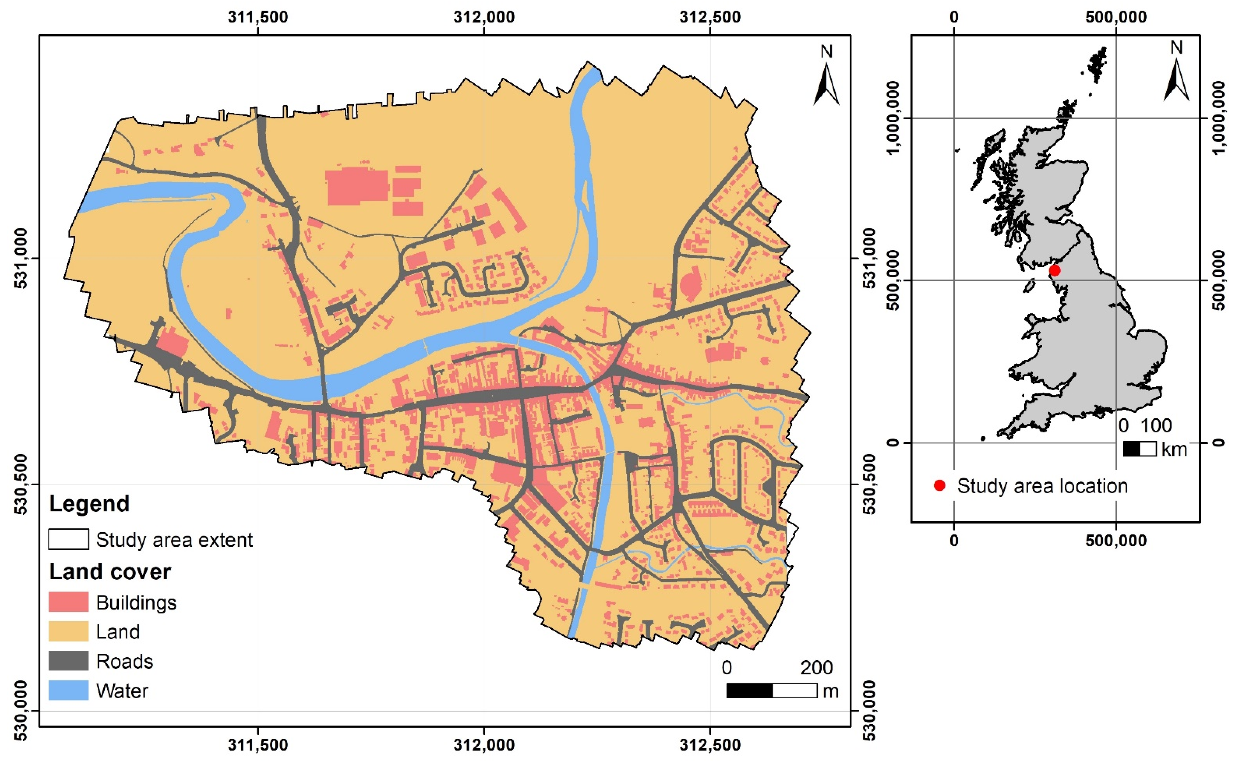
The study area is located in the town of Cockermouth, Cumbria, UK, at the confluence of the rivers Cocker and Derwent (Figure 1). The town was affected by a severe flood event caused by Storm Desmond that took place on 5–6 December 2015, damaging 466 properties [19]. The event was a consequence of heavy rainfall over an extended period with more than 300 mm of rainfall over a 24 h period [19], which translated into flows in the Derwent River of 395 m3 s−1 at the Ouse Bridge gauging station and 170 m3 s−1 at the Cocker Southwaite River gauging station. The estimated annual exceedance probability for the observed event was less than 1% for both rainfall and river flows.
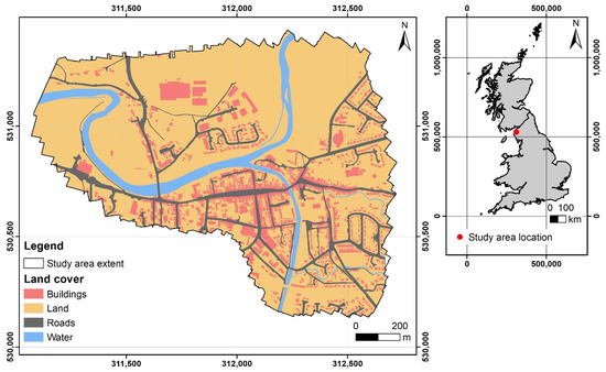
Figure 1.
Location of the study area with main land cover types depicted from aggregated classes of OS MasterMap Topography layer. The grid overlay is calibrated to British National Grid coordinates. [OS MasterMap® Topography Layer [FileGeoDatabase geospatial data], Scale 1:1250, Tiles: GB, Updated: 11 June 2015, Ordnance Survey (GB), Using: EDINA Digimap Ordnance Survey Service, Available online: https://digimap.edina.ac.uk, Downloaded: 10 November 2020 14:30:04.429].
2.2. Data
This study is based on a high resolution (0.1 m) UAV orthoimage in the visible light spectrum captured a week after the storm event, on 13 December 2015, over an area of 142 ha with a Sirus-Pro (Topcon Positioning System Inc., Livermore, CA, USA) fixed wing platform. The horizontal and vertical position accuracy of 0.01 m and 0.015 m, respectively, were ascertained by the Real Time Kinematic Global Navigation Satellite System GNSS-RTK---L1/L2 GPS and GLONASS (Global Navigation Satellite System) with RTK mounted on the platform. The camera was a 16-megapixel Panasonic GX-1 with 0.03 m pixel size, 14 mm focal length and Micro4/3 sensor type. The images were captured with 85% along and 65% across track accuracy at a speed of 65 km h−1 and at 112 m altitude with resulting ground sampling distance of 0.026 m. Further details regarding the UAV data acquisition are available in [6]. All the imagery was collected by a qualified pilot following airspace regulation. An ancillary data set with the location of the centroid of six random ground control points (GCPs) was obtained with a Topcon HiPer V GPS (Topcon Positioning System Inc., Livermore, CA, USA).
Interpretation of the main land cover classes present within the study area was facilitated by the OS MasterMap topographic map at the scale of 1:1 250 updated on 11 June 2015.
2.3. Photogrammetric Process
The quality and spatial coverage of each of the UAV images collected was inspected prior to their inclusion in the photogrammetric process. Individual frames that were distorted or blurred, did not present a nadir orientation and did not cover the area of interest were discarded. The geomatic products were obtained using Photoscan Pro version 1.1.6 (Agisoft LLC, St. Petersburg, Russia). Each individual frame was located, translated, and rotated into the World Geodetic System WGS84 for georeferencing purposes. The coordinates of the GCPs centroids were used to minimize distortion. The coregistration error was automatically derived from Photoscan Agisoft following [6]. From the geomatic products obtained i.e., orthoimage, point cloud and digital elevation model), only the orthoimage was used for the purpose of this study.
2.4. Object-Oriented Image Classification
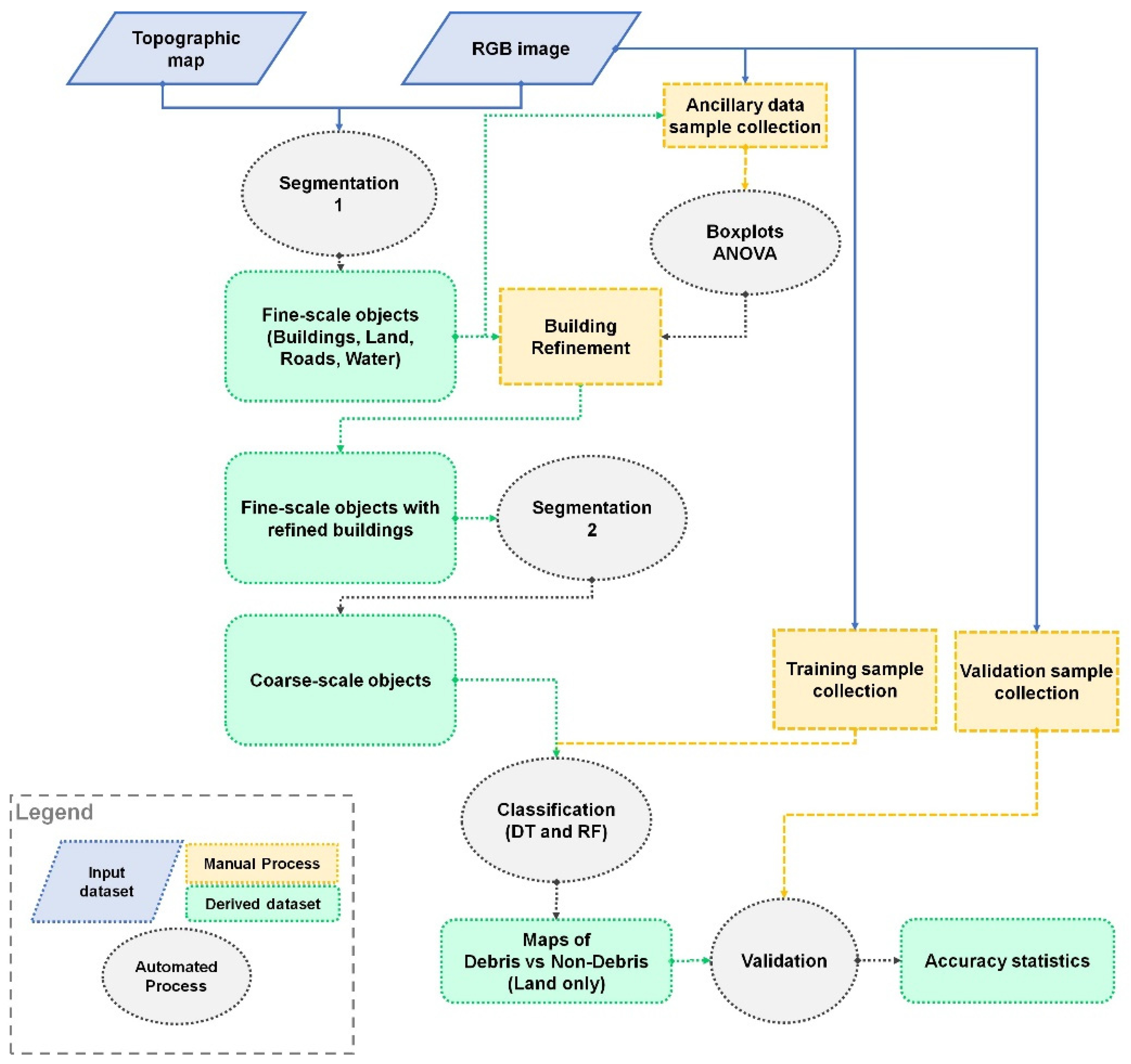
The methodology applied to detect debris indicative of flood damage to residential properties was based on object-oriented classification implemented within the eCognition Developer v10 (Trimble Geospatial, Munich, Germany) software (Figure 2). Supporting GIS tasks were carried out using ArcGIS Desktop v10.6 (ESRI, Redlands, CA, USA) and statistical analyses were conducted in R (R Foundation for Statistical Computing, Vienna, Austria) [20]. The methodology comprised two distinct steps: image segmentation and flooding damage classification, described Section 2.4.1 and Section 2.4.2 below.

Figure 2.
Workflow of the method applied for classification of flood debris. DT—decision trees, RF—random forests, RGB—red-green-blue image bands, ANOVA—analysis of variance.
In remote sensing, image classification can be carried out on pixel- or object-basis whereby a class value is assigned either to individual grid cells of an image or objects representing groupings of pixels possessing similar spectral properties. Object-based approaches are often cited as having a superior classification accuracy [21]. Image objects are created during the image segmentation process aimed at minimizing internal object heterogeneity with regards to set criteria. Multiple segmentation techniques exist, three of which have been used in this study: multiresolution segmentation, spectral difference segmentation and vector-based segmentation.
In multiresolution image segmentation techniques, which allow for segmentation of multi-band images taking into account spectral and textural properties of objects, homogeneity criteria are determined by parameters of scale, color, shape and compactness [22]. Scale determines the maximum allowed heterogeneity for the resulting image objects by defining the maximum standard deviation of the homogeneity criteria for each image band, with larger values yielding larger objects. The size of resulting objects will depend on the level of homogeneity within the image, with the same scale value yielding larger objects for more homogenous data. Color and shape define the importance weights of the spectral information of the image versus texture of resulting objects contributing to the homogeneity criterion. Compactness defines shape and can be used to separate compact from fractured objects that have similar spectral values.
Spectral difference segmentation merges neighboring image objects based on the maximum spectral difference value determined by the user, defined by the differences in mean intensity of the objects. Vector-based segmentation is used to convert vector thematic layers into objects retaining the shape and size of polygons.
Object-oriented image classification is carried out on objects derived during segmentation process and is based on the values of features that may be related to their spectral, geometric, and topological properties, among others. Spectral features refer to the statistical descriptors of the image’s pixel values for each available image bands, such as mean, mode and standard deviation. Spectral properties of image bands can also be used to describe texture of objects from the grey-level co-occurrence matrix (GLCM) defining the frequency at which different combinations of pixel gray levels occur in the scene. Geometry features constitute a large pool of descriptors related to the extent and shape of objects, polygons derived from objects or skeletons drawn within objects. Topological features describe the position of an object with regards to other objects, taking into account both their spatial and spectral properties.
2.4.1. Image Segmentation and Building Refinement
Image segmentation was carried out with the purpose of deriving homogenous objects depicting flood damage, referred throughout this manuscript to as debris, as well as remaining land cover features (i.e., non-debris). The segmentation and subsequent debris classification were necessarily facilitated by incorporation of main land cover classes (buildings, land, roads and water) depicted by the large-scale topographic OS MasterMap to avoid misclassification between buildings and their immediate surroundings. Whilst the topographic map helped to distinguish buildings from their surrounding land, it also provided excessive detail in terms of locations of large-scale features such as footpaths or structures, and these were incorporated into the principal land cover classes of land, buildings, roads and water. The procedure used is described in Table S1 of Supplementary Materials. Therefore, in the first step ‘vector-based segmentation’ process was used to derive objects corresponding to the major land cover classes as depicted by the topographic map. Objects representing classes ‘land’ and ‘buildings’ were further sub-divided during the ‘multiresolution segmentation’ process that used the RGB bands of the Cockermouth UAV image. The scale, shape and compactness parameters required for the segmentation were set to 10, 0.5 and 0.5 during a trial-and-error approach, calibrating the segmentation process so that the derived objects offered good separation of debris and non-debris features, and preventing the debris objects from comprising low-contrast features associated with their background when the scale parameter was set to larger values. Water and road objects were excluded from the multiresolution segmentation due to a very low presence of debris within these features.
The land cover features depicted by the topographic map and the UAV image were misaligned with regards to each other due to existing co-registration errors. The resulting misalignment posed an issue especially for buildings due to the exposure of their walls, which, when brightly colored, could be easily confused with debris by the classification algorithms deployed in the subsequent steps of the analysis. Additionally, white features such as conservatories that frequently were classified as ‘land’ in the topographic map, where also likely to be misclassified as debris and therefore had to be incorporated into the ‘building’ class. Building refinement was carried out through a multi-step reclassification procedure, implemented via the ‘assign class’ algorithm that reclassifies objects through application of conditional statements related to their spectral and geometrical properties. For this purpose, an ancillary sample of objects representing roofs, dark land, tiling, conservatories, white walls, and heaps of debris was captured and attributed with 70 different descriptors available from eCognition. The types of objects included in the ancillary data sample represented land cover features located in high proximity to building roofs that were likely misclassified as roofs or debris. For example, dark land representing water-saturated bare ground or ground sparsely covered with grass was likely to be misclassified as darker parts of roofs, whilst tiling characterized with bright, yellow-to-orange hues, was often misclassified as brighter parts of roofs. On the other hand, brightly-colored conservatories and white walls were frequently misclassified as heaps of debris, that were typically white/bright in color, especially when the latter were placed immediately next to the buildings. Selection of descriptors types and their values that offered the best distinction between these classes was facilitated by the analysis of variance (ANOVA) and boxplots, respectively. Descriptors presenting statistically significant differences (p-value < 0.05) between building roofs and walls and the remaining classes were considered in the refinement. It is important to note that the goal of this step was to reduce the confusion between buildings and debris rather than identify exact boundaries of the buildings, allowing for a small amount of overspill of the class ‘buildings’ onto the adjacent land cover objects.
In the final segmentation step, objects located within areas belonging to class ‘land’ were coarsened with the ‘spectral difference segmentation’ algorithm, using the maximum spectral difference setting of 10 for the RGB bands and 3 iteration cycles. These parameters were carefully chosen to minimize joining objects depicting debris to objects representing non-debris features whilst reducing the overall number of objects present within the image to facilitate the classification process and data handling. Larger values would have resulted in joining objects depicting both the debris and non-debris features together, reducing the accuracy of the subsequent classification, whilst smaller values of these parameters would retain an excessive number of objects within the image, increasing the time needed for the deployment of classification models. The ‘merge region’ algorithm was also used to merge all fine-resolution objects belonging to class ‘buildings’.
2.4.2. Flood Damage Classification
Flood damage classification was carried out on coarse-resolution objects in three steps: sample collection, classification, and accuracy assessment, described in the Sub-Sections below.
Sample Collection
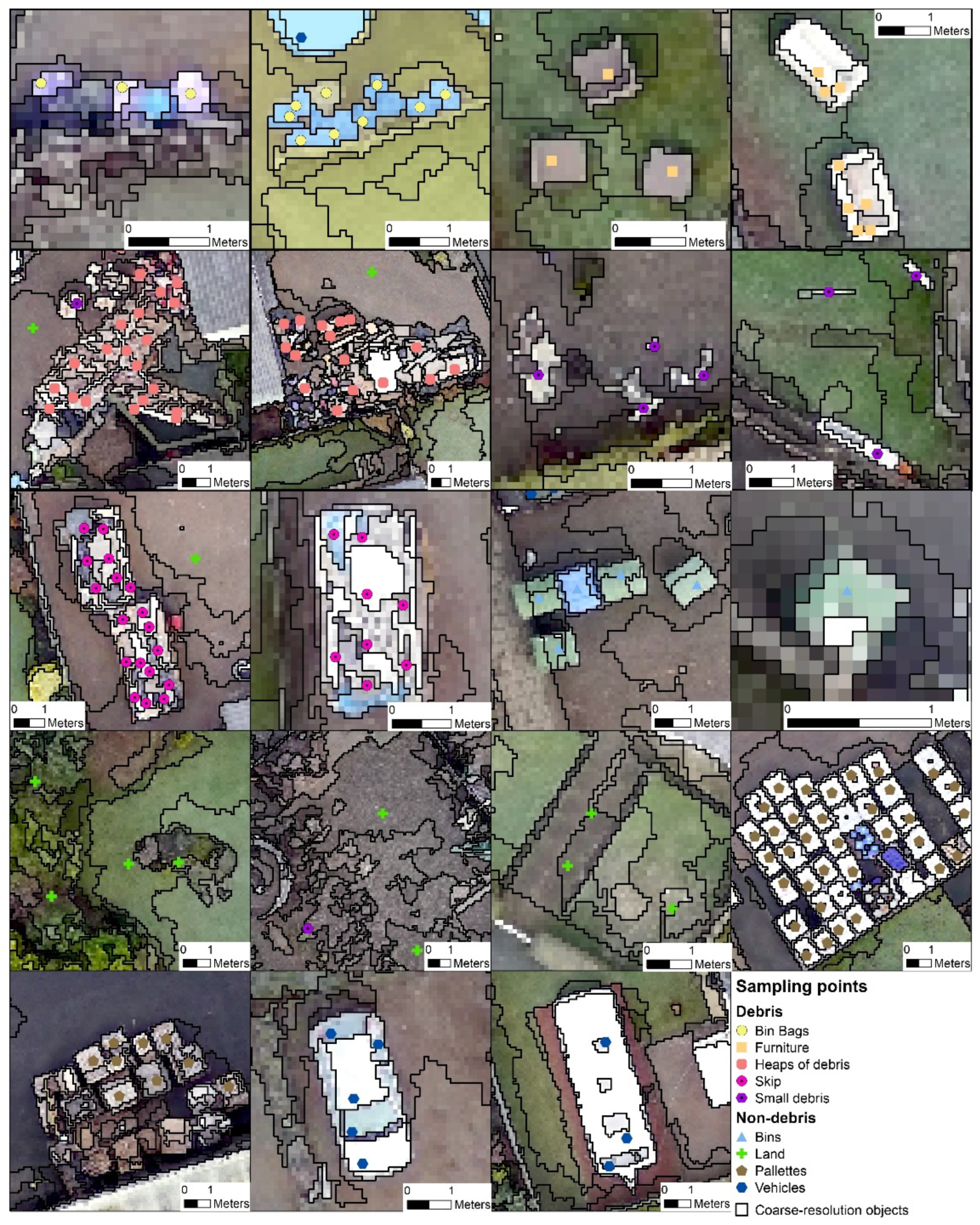
Point sample collection was carried out in ArcGIS Desktop environment upon careful inspection of the Cockermouth UAV image for different types of debris, and was informed by an existing image interpretation carried out for the purpose of a previous study [6]. The most prominent signs of flood damage comprised large heaps of debris representing water damaged goods stored in a high proximity to houses as well as skips containing such goods placed in the driveways or front gardens, however, also included small scattered debris, furniture left to dry outside, as well as multiple bin bags gathered in front gardens. For algorithm training and validation purposes, the data sample was supplemented with features that could potentially be confused with debris, which included bins, industrial palettes, cars, as well as objects representing tiling/paths, grass and bare ground of different shades, hedges, shrubs and trees. No samples were collected for road features or water, given that the subsequent classification was targeted at the ‘land’ class where the majority of the debris were located. Figure 3 shows examples of debris and non-debris features.

Figure 3.
Examples of debris and non-debris data samples.
Prior to classification, the sample was divided into approximately 70–30% sub-samples, used for model training and validation, respectively (Table 1). Purity of the samples was ensured by visual inspection of the coarse-resolution objects intersecting with the samples and removal of any points placed within objects containing both the debris and the surrounding land. Whilst the training sample was only drawn from areas classified as ‘land’, the validation sample covered both features within ‘land’ and the refined ‘buildings’, allowing for assessment of accuracy including the potential overspill of buildings into adjacent debris during refinement. Additionally, only one point per object was retained in cases where multiple points were placed within an object during sample collection. Finally, the different types of flooding damage identified during the sample collection, were amalgamated into debris and non-debris classes prior to training of the models.

Table 1.
Model training and validation samples types and sizes expressed as number of coarse-resolution objects. Values in brackets refer to the proportion of the total sample size used for model training and validation. NV—samples excluding vehicles, WV—samples including vehicles.
Classification
Classification of objects related to debris and non-debris features was carried out in eCognition Developer software using tree-based classifiers. Tree-based classifiers are machine learning methods that can be used to generate prediction models from tabular data, and have exhibited high performance levels in land cover classification problems [23,24] including classifications of very high resolution imagery in urban settings [25,26]. Decision trees, being an implementation of classification and regression trees (CARTs) [27], and random forests (RF) [28] were used in this study. In general, tree-based classifiers recursively partition the data to fit a simple prediction model within each partition so that a tree-like decision structure is created, with branches representing pathways through splits of predictor values and the leaves—the target classes associated with these values [24,29]. Whilst the DT algorithm derives a single tree from the dataset that clearly visualizes the classification rules and is fast to implement, RFs make the final decision based on the majority vote from multiple trees that use a random subset of observations and predictor variables, and are therefore difficult to visualize. RFs, however, do not overfit data, as opposed to other machine learning methods used in urban flood mapping such as artificial neural networks, do not require the input variables to be normally distributed as is the case in maximum likelihood methods, and are quicker to parameterize than support vector machines [26]. RFs can also provide an unbiased estimation of accuracy as well as relative importance of each variable used in the prediction.
In this study, regardless of the algorithm used, classification of the UAV image into debris and non-debris features was carried out in two steps. Firstly, DT and RF models were trained with coarse-resolution objects derived during the second step of image segmentation that intersected with training points locations captured during visual interpretation of the image. These objects were attributed with multiple spectral and geometrical properties available in the eCognition Developer software (Table S4 Supplementary Materials). Both the DT and RF models were trained twice, with or without vehicles included in the training sample using settings shown in Table 2 below.
Table 2.
Settings used to train the random forests (RF) and decision trees (DT) models, with training data sample excluding (WV) and including (NV) vehicles; n/a refers to settings not applicable to the algorithms.
The parameters of depth and minimum sample count, both set to 0 in the RF and DT algorithms, did not constrain the trees in terms of their depth as well as the allowed number of observations at each node. Given that the data sample did not contain any missing values, there was no need for the algorithms to use surrogate splits to predict actual splits of the data. The maximum categories parameter refers to the number of clusters used in categorical variables, which in the case of this study was spurious due to all predictors being continuous. The DT algorithm was pruned during 10 cross-validation folds, reducing the likelihood of overfitting our data. No additional pruning due to the application of 1 SE rule, selecting the smallest tree with estimated error smaller than the lowest estimate of error increased by 1 standard error of this estimate, was applied. Finally, no truncation of the pruned tree was requested, allowing for the retrieval of non-truncated branches. In the RF algorithm settings, the active variables parameter of 0 allowed for a random selection of the square root of the total number of predictive variables at each tree node, which is a default setting used by the algorithm. The maximum tree number was set to a large number of 500 allowing for the forest to minimize the out of bag error before reaching the termination criteria, which were set to both criteria of achieving the maximum number of trees as well as the sufficient forest accuracy. Sufficient forest accuracy was set to a low value of 0.01% not to constrain the evolution of the forest.
In the second step of the classification, the trained models were deployed on all coarse-resolution objects covering land depicted by the topographic map to yield four different classified maps in total.
Accuracy Assessment
Given that our flood damage detection approach aimed at classification of debris vs. non-debris features, accuracy assessment was carried out with binary confusion matrices derived with the ‘caret’ library [30] in R software. An independent validation data sample was used. Confusion matrices allow for calculation of multiple metrics for diagnostics of performance of a classification scheme. These include overall accuracy (ACR) (Equation (1)), sensitivity, i.e., true positive prediction rate (TPR) expressing the ratio of correctly classified positive samples (P) (Equation (2)), specificity, i.e., true negative prediction rate (TNR) expressing the ratio of correctly classified negative samples (N) (Equation (3)), precision and inverse precision, i.e., positive and negative prediction values (PPV and NPV), measuring the proportion of correctly classified positive or negative samples to the total number of positive or negative samples (Equations (4) and (5)), prevalence (PRV), indicating the proportion of the positive samples in the data (Equation (6)), detection rate (DT) (Equation (7)) measuring the rate at which positive values were correctly classified, detection prevalence (DPRV) (Equation (8)), and balanced accuracy (BACR) (Equation (9)) correcting the accuracy score for an imbalanced data sample. In this study, p values refer to samples of debris and N values refer to non-debris features. The notation of equations was adapted from [30,31]. Additionally, the unweighted Cohen’s kappa coefficient was calculated (Equation (10)) [32].
3. Results
3.1. Refinement of Buildings
The ANOVA (Table S2 in Supplementary Materials) carried out for pairs of different land cover features considered in the building refinement procedure over multiple spectral and geometrical properties of fine-resolution objects, identified eleven descriptors that, based on statistically different means (p-value < 0.05), could be helpful in discriminating between buildings and other land cover features. These descriptors included brightness, mode (maximum) of the RGB image bands, length of the border to buildings, relative border to buildings, width, relative border to land, distance to buildings, asymmetry, GLCM contrast in all directions, and length/width ratio. Boxplots plotting the range of values of these descriptors for each land cover class considered in the procedure (Figure 4), however, revealed that some overlap was present between roofs or white walls and the remaining features. The size of the overlap varied depending on the descriptor and land cover feature, however, roofs could appear similar to adjacent dark land and tiling, and white walls to heaps of debris and conservatories.
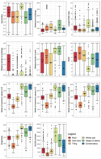
Figure 4.
Boxplots depicting the discriminatory variables between building roofs and adjacent land cover features used in the building refinement procedure. Points outside the interquartile range represent both outliers and extreme values.
The 13-step building refinement procedure (Table S3 in Supplementary Materials) was primarily based on brightness and maximum mode values of the RGB bands, classifying objects that were moderately bright, and brighter in the B than R image band as roofs, with the remaining descriptors acting as refining variables. Importantly, white walls were set apart from brightly colored debris through their width.
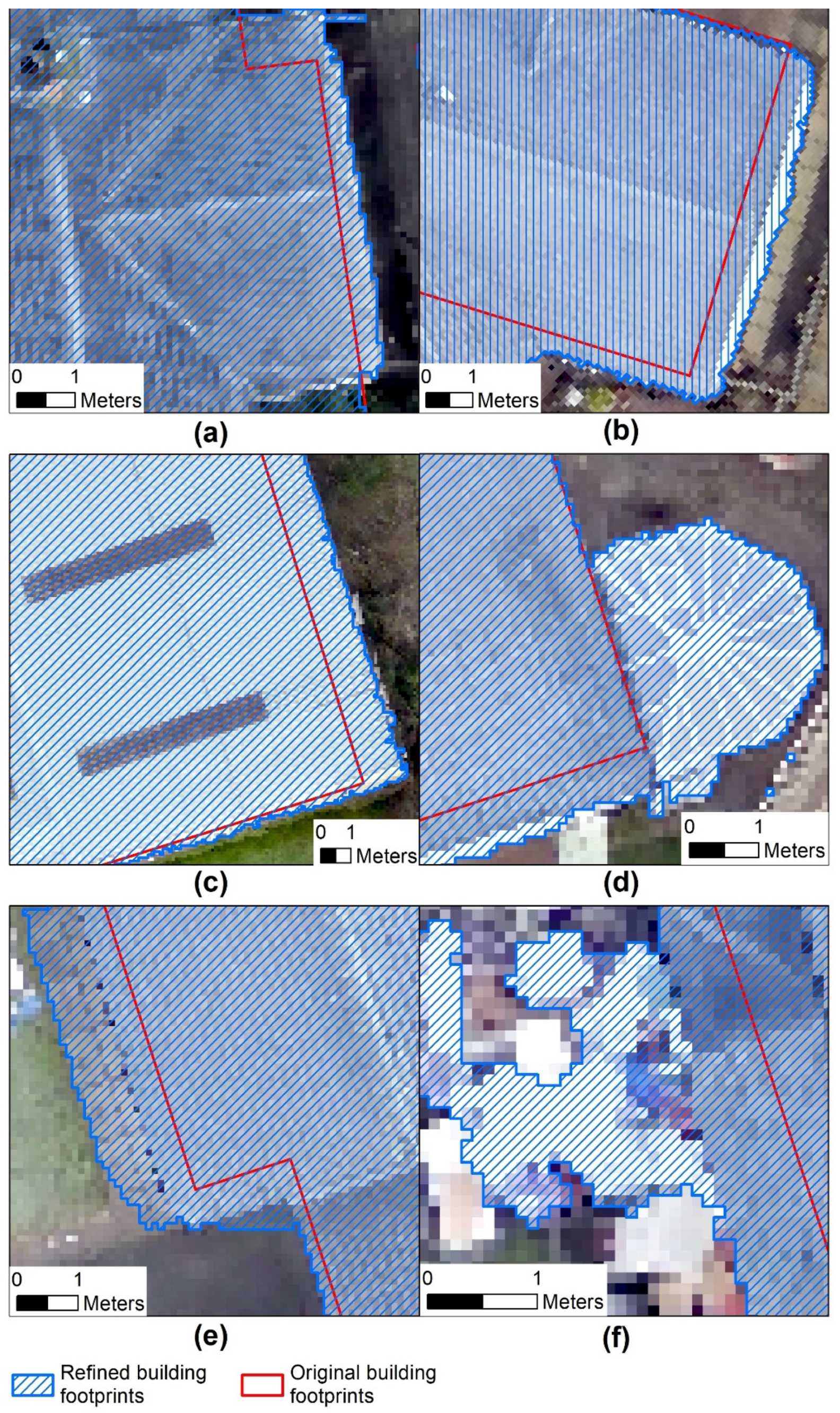
Visual inspection of the outcomes of the procedure showed that in overall it was successful at improving the delineations of building footprints including conservatories (Figure 5). Despite the implementation of the numerous refinement steps with carefully selected thresholds informed both by the boxplots and a trial-and-error approach, however, some tiling immediately adjacent to buildings as well as debris was erroneously classified as buildings. Given that the principal goal of this classification was to separate buildings from debris rather than accurately represent building footprints, some misclassifications between buildings and adjacent paving or the ground were allowed. Any confusion with the debris, however, was not desirable and was captured during validation of the flood damage classification results presented in Section 3.2.
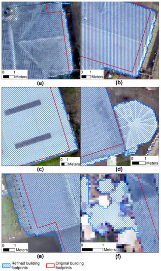
Figure 5.
Outcomes of the building refinement procedure aiming at the reduction of the misclassification rate of flooding debris into buildings. Images (a–d) show accurately refined buildings, including white walls (b) and conservatories (d). Images (e,f) show examples of buildings overspilling onto adjacent pavement or debris following the procedure.
3.2. Classification of Flooding Damage
3.2.1. Classification Accuracy
Numerical assessment of the accuracy of the classification of image objects into classes representing flood damage, i.e., debris, and other land cover features, i.e., non-debris, (Table 3), indicated that the random forest model trained with data sample that excluded vehicles was most successful at depicting debris, with the overall accuracy of 74%, (p-value < 0.001). The value of specificity metric of 0.82, however, indicated that the model was more successful at classifying features belonging to the non-debris class, and the sensitivity metric indicated that only 58% of the debris was successfully classified.
Table 3.
Accuracy assessment for debris classifications obtained with the random forests (RF) and decision trees (DT) algorithms with exclusion (NV) or inclusion (WV) of vehicles in the training data sample. In the assessment, positive value was set to ‘Debris’.
Decision tree models were not successful at depicting the debris, which could be associated with only two predictor variables (contribution of the green image band to overall brightness and border length of image objects) being included in the tree structure, likely resulting from excessive pruning during the 10-fold cross-validation process. All models trained with the data sample containing vehicles were unable to detect debris within the image, indicating high levels of confusion between vehicles and debris features. Inspection of the map obtained from the RF model that excluded vehicles during training revealed that brightly-colored vehicles, including cars, vans or camper vans, were typically misclassified as debris. In fact, the brightness of color was a decisive factor for classification of objects as debris, with darker debris not being picked out in the classification.
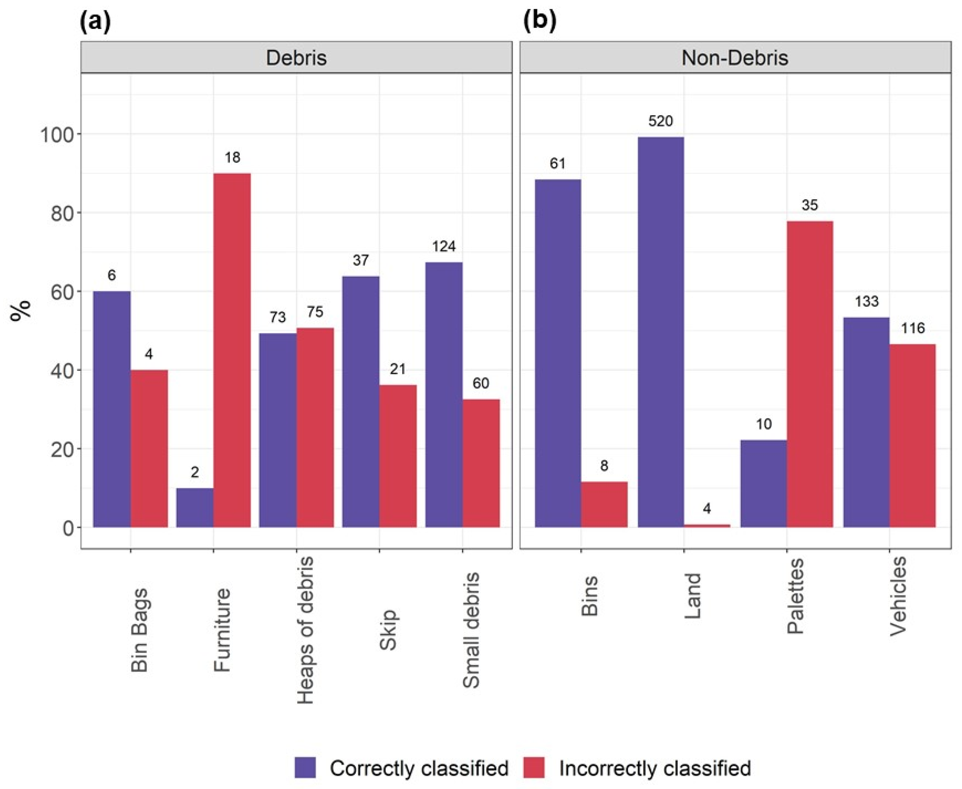
Analysis of the distribution of the correctly and incorrectly classified features (Figure 6) revealed that out of the different debris types, small debris followed by heaps of debris and skips were most accurately classified, and pieces of furniture were least accurately represented by the random forest model. Amongst the non-debris features, a great majority of objects representing land and bins were correctly classified. Approximately half of the vehicles as well as the majority of industrial palettes were misclassified as debris. Finally, fragments of the RF image showing correctly and incorrectly classified debris are shown in Figure 7.
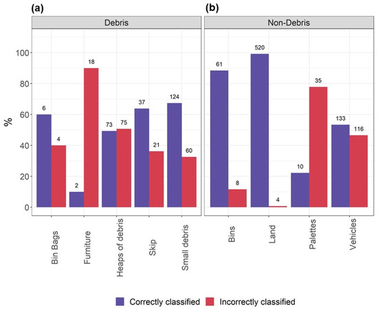
Figure 6.
Distribution within the validation data sample of correctly and incorrectly classified land cover features representing (a) debris and (b) non-debris split into their respective feature types for the random forest model trained with data sample excluding vehicles. Counts of objects falling into the correctly or incorrectly classified categories are shown above the bars.
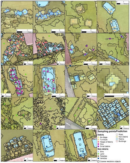
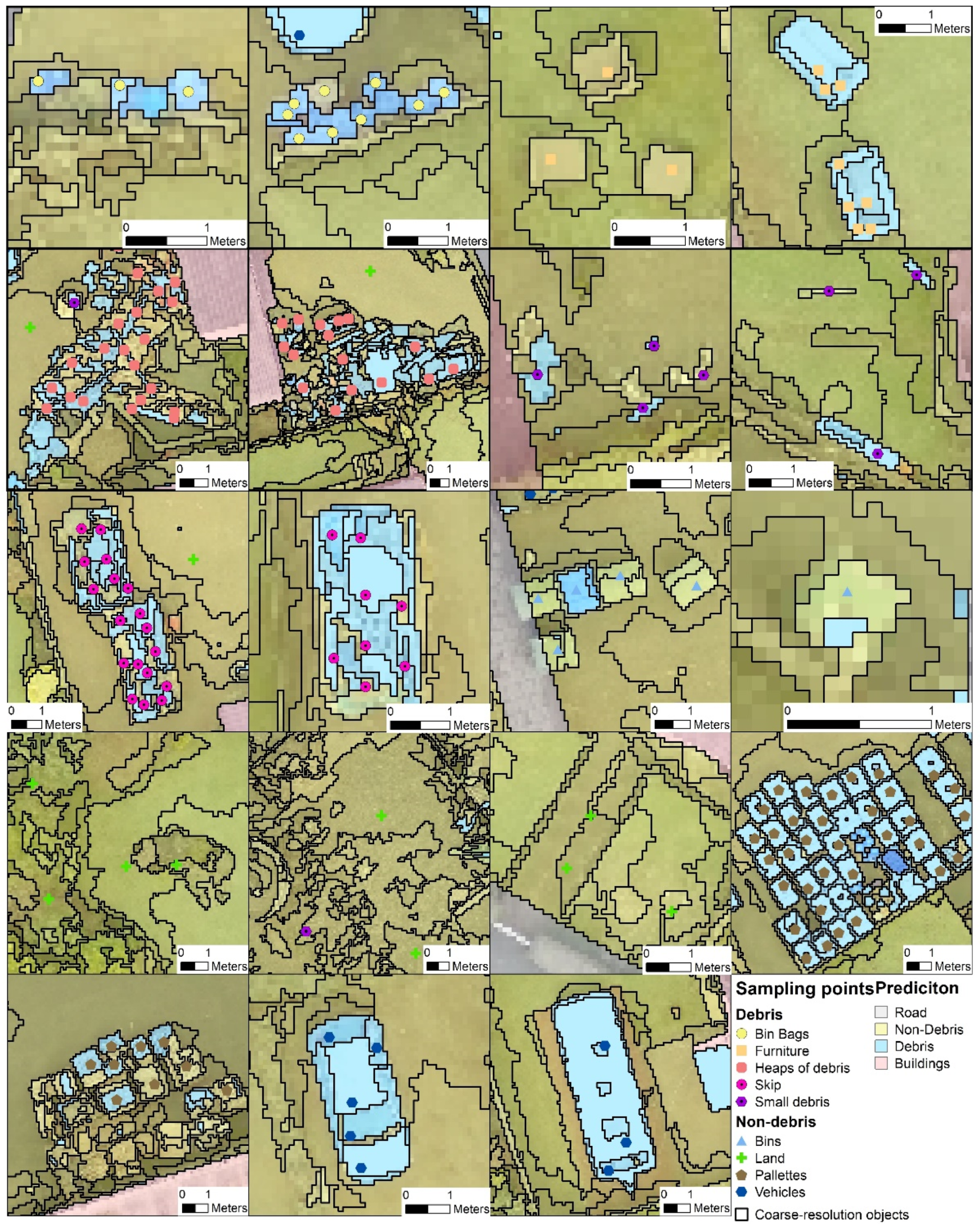
Figure 7.
Fragments of maps of debris and non-debris features predicted with RF model trained with data sample excluding vehicles. The correct label of an object is provided by the sampling points displayed in the figure.
3.2.2. Variable Importance
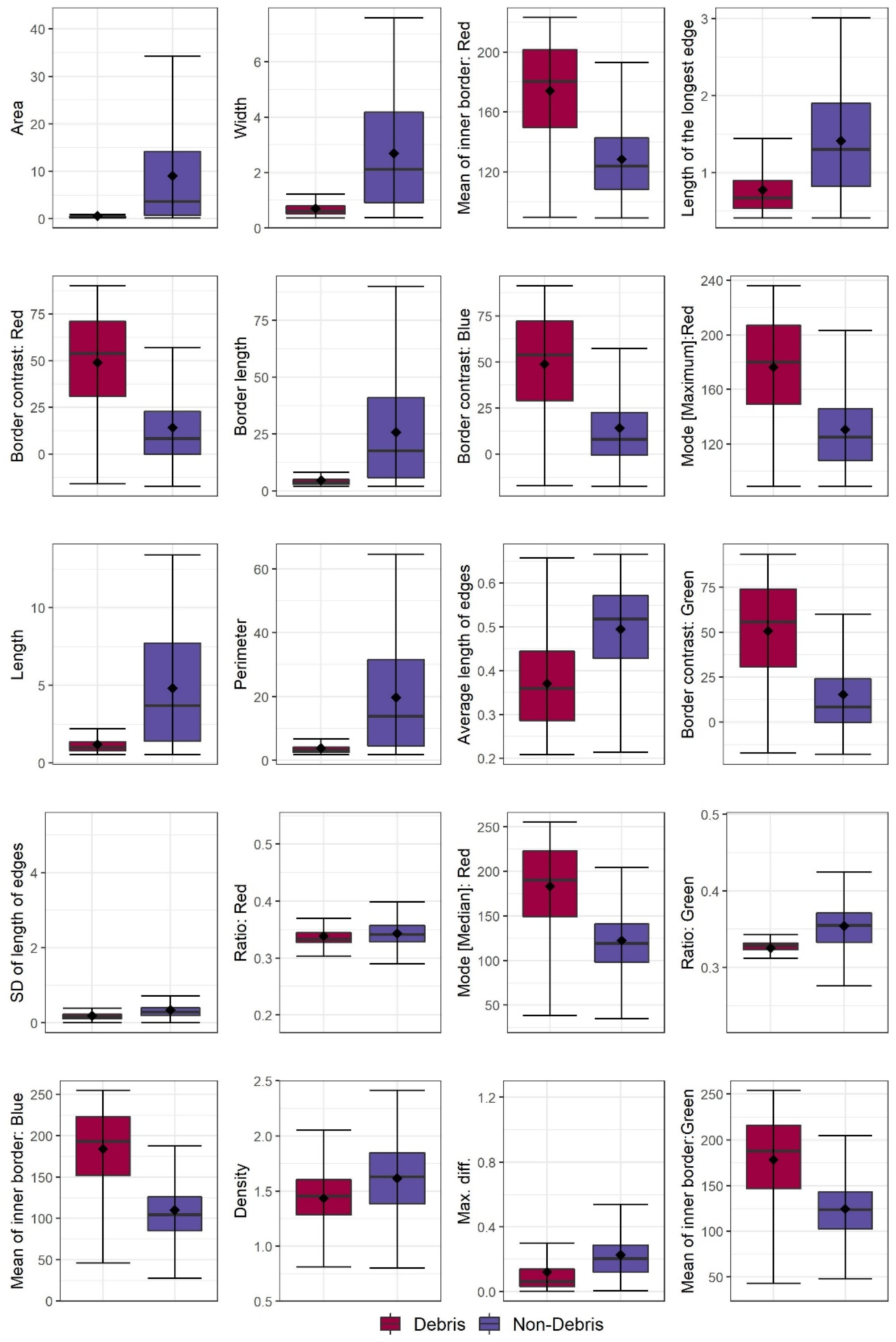
The list of variable importance of the random forest model constructed with the training sample excluding vehicles pointed to a high variety of spectral and geometrical properties of objects useful for making a distinction between debris and other features in our study area setting (Table 4). The most important variable used in the classification was “area” expressed as the number of image pixels forming an image object, closely followed by “object width”, both referring to the geometric properties of image objects. The third most important variable was the “mean value” of the red image band of the pixels forming the inner border of an object, referring to the objects’ spectral properties. Out of the arbitrarily chosen top twenty predictors and metrics representing spectral properties of the image objects, the red band was used most frequently, with five different metrics, followed by the green band (three metrics) and blue band (two metrics). Both the spectral and geometric properties of the objects were equally important, given the near equal distribution of metrics belonging to these categories within the top twenty predictors. The distributions of these predictors for debris and non-debris features are shown in Figure 8, with the debris typically associated with relatively higher values of spectral and lower values of geometric properties as compared to non-debris, corresponding to their brighter color and smaller size.
Table 4.
Top twenty most important predictors of flood damage identified by the random forest model. The full list of predictors is given in Table S4 in Supplementary Materials. Letters R, G, and B refer to the red, green and blue bands of the Unmanned Aerial Vehicle (UAV) image. Variable type refers to its capacity to describe spectral (Sl) or geometric (Gc) properties of an image object. Variable definitions are based on [22].
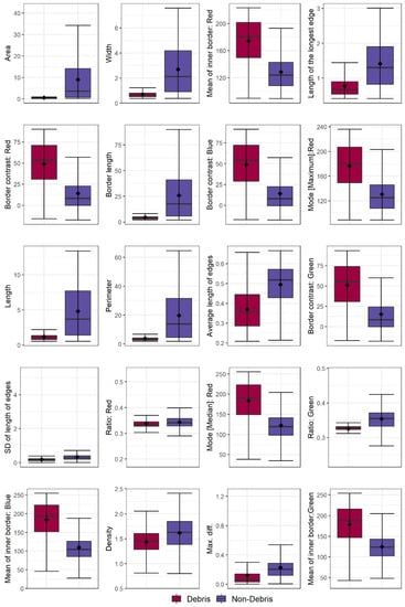
Figure 8.
Distribution of the top 20 predictor variables of debris and non-debris features identified by the random forest model training dataset excluding vehicles. Predictor descriptions are given in Table 4.
4. Discussion
4.1. Flood Damage Detection
This study aimed at the development of a combined OBIA-ML-UAV system engineering solution for automated identification of flood impact to residential properties with the purpose to facilitate rapid screening for damaged properties and consequently reduce the time needed for insurance assessments. As such, out of different types of flood damage identified during a visual interpretation of the available image during a previous study [6], features representing natural debris e.g., sediment deposits, trees, branches and other types of organic matter deposited across the study area; scour, leftover water pools as well as signs of damage to infrastructure including exposed pipes and bridge barriers were excluded from the analysis. Instead, we focused on detection of water-damaged goods removed from affected households stored next to the houses (heaps of debris) or placed in skips located in the front gardens. Scattered smaller pieces of debris, house furniture placed outside of houses and bin bags filled with damaged goods were considered in the final classification as well.
Our classification approach required selection of objects representing land cover features not associated with flood damage. These included different types of natural land cover (grass of different shades, trees or shrubs with and without leaves) as well as items that were frequently misclassified as debris in preliminary classifications (bins, industrial palettes, and vehicles). Our training dataset did not include any samples related to buildings, roads or water, given that these areas were excluded from the classification as the vast majority of the debris associated with households were located in class ‘land’ depicted by the topographic map and effectively constraining our methodology to sub-urban type residential properties surrounded by gardens. Although the overall accuracy rate for the classified image was 74%, the random forest algorithm was more successful at correctly classifying features representing non-debris classes (80%), with debris being correctly classified at the rate of approximately 60%. Inspection of the resulting predictive map and the original UAV image revealed that debris was more likely to be correctly classified when it was brightly-colored, ensuring distinct contrast to the surrounding land. Conversely, fragments of debris similar in color to their immediate surroundings where either not delineated correctly during segmentation process or misclassified. These results are consistent with those reported in [13] where a convolutional neural network was used to detect water-related disaster damage with an overall accuracy of 77.01% for the bulk classes such as the flooded area, vegetation and roads, and 51.4% for the countable classes (e.g., damaged and not damaged building roofs, cars, and debris).
High levels of confusion also occurred between debris and brightly colored vehicles, which were frequently confused with skips. In fact, confusion with vehicles was very prominent pointing to the inability of the deployed algorithms to detect debris within the image when objects corresponding to vehicles were included in the training datasets. This is confirmed by a greater degree of overlap between values of the most important predictors of debris and non-debris features in training data sample including vehicles as compared the data sample excluding vehicles (Figure S1 Supplementary Materials).
Given that flood-affected houses in the study area were associated with both bright and dark debris, the moderate detection accuracy achieved in this study was sufficient to identify properties that suffered flood damage. Post-classification visual inspection of the image would have to be deployed, however, to identify vehicles incorrectly classified as debris to avoid misidentification of undamaged houses.
Lower accuracy of detection of debris than non-debris features could be associated with an imbalanced sample of these features used in the model training. ML algorithms, including tree-based classifiers, may be sensitive to imbalanced training data samples, i.e., samples containing an unequal number of observations in each class. This may lead to predictions of the most dominant category only, especially in binary classification problems [24], which was the case in our study. Nevertheless, given that debris to non-debris ratio of 1.3 and 2.1 for training samples excluding and including vehicles did not exceed the factor of 4 or more, which can be considered as a severe imbalance [33], we attribute the lower detection rate of debris to class overlap, especially when vehicles were included in the data sample. Consequently, further improvements should focus on deployment of more robust models for prediction of imbalanced data as well as an enhanced description of the land cover features to reduce confusion, e.g., via further refinement of objects representing debris and non-debris features
4.2. Implications for Flood Impact Assessment
The automated method for flood damage detection from UAV imagery presented in this study could facilitate rapid screening of flood-affected areas for signs of damage to houses, given the availability of processed UAV imagery. Manual detection and classification of flood damage in the same study area took 132 h in total, 36 h of which were dedicated to the photogrammetric process required to process the collected UAV imagery, 72 h for digitization of impact features and 24 h for estimation of losses [6]. The automated method developed here reduced the detection time of debris from 72 h to circa 98 min, of which 48 min was dedicated to image segmentation within buildings and land covering an area 119 ha in size, 27 min to building refinement and coarsening of objects, 12 s to training and 22 min to deployment of the RF model from pre-collected training data run on a 64 GB Lenovo® UK PC with 2 Intel® Xeon® 4110CPU @ 2.10 GHz processors. Given moderate accuracy of our approach, which may be hindered by specific properties of a different study area and data, additional time should be allocated for manual reclassification of incorrectly classified objects.
The times needed for automated debris detection may significantly be increased when a training data sample needs to be collected, involving visual interpretation of the UAV imagery. In such cases we recommend visual inspection and sample collection from a representative portion of the study area where most of the damage had occurred, for example by random selection of 50% of quadrants sized proportionally to the size of the affected area to reduce the time needed for the analysis. Additionally, to ensure good predictive power of the RF model, care should be taken to collect a balanced sample of objects representing debris and non-debris features [34]. This can be achieved by application of sampling strategies aiming at equalization of the numbers of observations for each class, such as for example under-sampling of overrepresented features or synthetic over-sampling of minority features, discussed in [35].
UAV imagery has been used for flood extent and associated damage assessment as well as rescue operations, allowing for rapid and safer actions immediately after or during the event [36]. In our context, however, the successful flood damage detection requires flood water to retreat and the area to be safe enough for people to return and clear out their homes from damaged goods that can be subsequently detected within the imagery. Consequently, UAV survey needs to be timed well with clearing out activities that happen days after the flood occurred. In the light of the door-to-door inspections for insurance purposes having to take place before the debris can be removed, the risk of it being cleared out completely causing non-detection is currently small but may increase in the future when automated damage detection methods are adopted.
4.3. Future Work
Future attempts for object-based classification of flood damage could benefit from inclusion of the near-infrared spectral band at both the image segmentation and classification stages to help mitigate the confusion between debris colored with hues of green and brown and the surrounding vegetation that occurred in this study. The green pigment contained within plant cells, chlorophyl, has a distinctly high reflectance in the NIR light spectrum, which is absent from artificial pigments, and therefore may provide sufficient contrast to the natural land cover. Conversely, inclusion of surface elevation data derived from stereo-pairs of the UAV images (nadir and oblique) in addition to the digital elevation model obtained from the photogrammetric process could help with accurate detection of buildings as well as reduce confusion between lightly colored debris and other bright features, and sheds and stand-alone conservatories in particular, whose height is typically greater than that of debris. Note that the inclusion of any surface elevation information would require an ancillary data set of accurate elevation measurements for validation purposes.
Moreover, application of different types of algorithms, including deep learning should be considered in future studies. For example, different architectures of deep learning algorithms were successful at accurately classifying complex urban land cover from objects derived from high-resolution imagery, with the caveat that state-of-the-art ML methods such as gradient boosting trees or support vector machines, less dependent on large training samples, performed comparably well [37]. To facilitate the deployment of computer vision algorithms such as convolutional neural networks and other ML algorithms, we have generated a library of image objects [10.17862/cranfield.rd.14816355.v1], available upon a reasonable request, containing visual and tabular samples of the different types of debris detected in this study. The transferability of application of our debris libraries will depend on spatial resolution of the UAV image available, time of year the flood event occurred and/or climatic zone determining the development stage of green vegetation, and on-the-ground moisture conditions affecting the saturation of color of land cover features depicted by the image.
4.4. Limitations and Reproducibility of the Results
The main limitation of this study relates to the fact that the image segmentation parameters used to derive objects were tailored to the specific properties of our UAV image in terms of spatial resolution and altitude of the sensors affecting the scaling between actual and represented size of ground features and invoking the need to modify parameters used in this study. Conversely, both the building-refinement procedure and the tree-based classification approaches relied on the RGB values of the image, which may be altered with different season of the year, weather, and physiography of the study area. Should these differ largely from our data, a new training sample of objects would have to be captured. Moreover, implementation of our procedure requires a certain level of expertise in handling of geospatial data that may necessitate outsourcing of the task to appropriate consultants or employment of geospatial analysts, both incurring additional costs to insurance companies. Alternatively, the procedure could be packaged into a user friendly and flexible software solution, for example with the use of eCognition Architect software, facilitating implementation of existing object-oriented image classification solutions to new study areas by non-specialists.
5. Conclusions
This study presents an automated method for object-based UAV image classification aimed at detection of flood damage to residential housing with the overarching aim of shortening the time needed for damage assessment for insurance purposes. Object-oriented classification of a very high resolution RGB image with the use of the random forest algorithm was able to detect items damaged during the flood and removed from houses fairly well provided that the debris was lightly colored. Darker items provided insufficient contrast to the land surface predominantly composed of wet soil, sediment and grass and were omitted by the process. Additionally, some brightly-colored land cover features were misclassified as debris. Consequently, we propose that the presented procedure can aid visual interpretation of an UAV image at the screening stage for signs of flood damage, however, is not sufficiently accurate to replace it entirely. Future improvements to the classification should consider inclusion of multispectral imagery as well as surface height data to reduce confusion between land surface features representing debris and non-debris as well as implementation of deep learning methods such as convolutional neural networks. When successful, automated flood damage detection methods can assist the estimation of insurance costs for insurance companies as well as identification of houses requiring inspections. Moreover, data on locations of housing affected by flooding can be used by appropriate agencies to devise risk management plans and implement tangible solutions preventing the damage from reoccurring. Similarly, in an event of another flood, emergency and rescue services could prioritize locations that are known to have suffered most severe damage in the past to increase their effectiveness and potentially save lives.
Supplementary Materials
The following are available online at https://www.mdpi.com/article/10.3390/rs13193913/s1. Table S1 Aggregation of land cover classes present in the OS MasterMap topographic layer used as an ancillary dataset in the automated procedure for detection of flood damage. Table S2 ANOVA analysis for selected descriptors of objects belonging to ancillary land cover classes used for refinement of buildings delineated by the topographic map. Table S3 Building refinement procedure. Table S4 Variable importance determined by the RF model trained with a sample that excluded vehicles. Figure S1 Distribution of the top 20 predictor variables of debris and non-debris features identified by the Random Forest model training dataset including vehicles.
Author Contributions
Conceptualization, J.Z. and M.R.C.; methodology, J.Z and M.R.C.; software, J.Z.; validation, J.Z.; formal analysis, J.Z.; investigation, J.Z.; resources, M.R.C.; data curation, M.R.C.; writing—original draft preparation, J.Z.; writing—review and editing, I.T., A.K., M.R.C.; visualization, J.Z.; supervision, M.R.C.; project administration, M.R.C.; funding acquisition, M.R.C. All authors have read and agreed to the published version of the manuscript.
Funding
This research was funded by Innovate UK, grant number 104880.
Institutional Review Board Statement
Not applicable.
Informed Consent Statement
Not applicable.
Data Availability Statement
The underlying data is confidential and cannot be shared.
Acknowledgments
We would like to thank Innovate UK for funding this project. We would also like to thank the reviewers for their useful and detailed comments. We believe the manuscript is easier to read and follow as a result.
Conflicts of Interest
The authors declare no conflict of interest. The funders had no role in the design of the study; in the collection, analyses, or interpretation of data; in the writing of the manuscript, or in the decision to publish the results.
References
- Kundzewicz, Z.W.; Kanae, S.; Seneviratne, S.I.; Handmer, J.; Nicholls, N.; Peduzzi, P.; Mechler, R.; Bouwer, L.M.; Arnell, N.; Mach, K.; et al. Le risque d’inondation et les perspectives de changement climatique mondial et régional. Hydrol. Sci. J. 2014, 59, 1–28. [Google Scholar] [CrossRef] [Green Version]
- Faulkner, D.; Warren, S.; Spencer, P.; Sharkey, P. Can we still predict the future from the past? Implementing non-stationary flood frequency analysis in the UK. J. Flood Risk Manag. 2020, 13, e12582. [Google Scholar] [CrossRef] [Green Version]
- Environment Agency. Flooding in England: A National Assessment of Flood Risk; Environment Agency: Bristol, UK, 2009. Available online: https://www.gov.uk/government/publications/flooding-in-england-national-assessment-of-flood-risk (accessed on 7 May 2021).
- Environment Agency. Estimating the Economic Costs of the 2015 to 2016 Winter Floods; Environment Agency: Bristol, UK, 2018. Available online: https://www.gov.uk/government/publications/floods-of-winter-2015-to-2016-estimating-the-costs (accessed on 11 July 2021).
- Sghaier, M.O.; Hammami, I.; Foucher, S.; Lepage, R. Flood extent mapping from time-series SAR images based on texture analysis and data fusion. Remote Sens. 2018, 10, 237. [Google Scholar] [CrossRef] [Green Version]
- Casado, M.R.; Irvine, T.; Johnson, S.; Palma, M.; Leinster, P. The use of unmanned aerial vehicles to estimate direct tangible losses to residential properties from flood events: A case study of Cockermouth Following the Desmond Storm. Remote Sens. 2018, 10, 1548. [Google Scholar] [CrossRef] [Green Version]
- Feng, Q.; Liu, J.; Gong, J. Urban flood mapping based on unmanned aerial vehicle remote sensing and random forest classifier-A case of yuyao, China. Water 2015, 7, 1437–1455. [Google Scholar] [CrossRef]
- Popescu, D.; Ichim, L.; Stoican, F. Unmanned aerial vehicle systems for remote estimation of flooded areas based on complex image processing. Sensors 2017, 17, 446. [Google Scholar] [CrossRef] [Green Version]
- Hashemi-Beni, L.; Gebrehiwot, A.A. Flood Extent Mapping: An Integrated Method Using Deep Learning and Region Growing Using UAV Optical Data. IEEE J. Sel. Top. Appl. Earth Obs. Remote Sens. 2021, 14, 2127–2135. [Google Scholar] [CrossRef]
- Ichim, L.; Popescu, D. Flooded Areas Evaluation from Aerial Images Based on Convolutional Neural Network. In Proceedings of the International Geoscience and Remote Sensing Symposium (IGARSS), Yokohama, Japan, 28 July–2 August 2019; pp. 9756–9759. [Google Scholar]
- Hashemi-Beni, L.; Jones, J.; Thompson, G.; Johnson, C.; Gebrehiwot, A. Challenges and opportunities for UAV-based digital elevation model generation for flood-risk management: A case of princeville, north carolina. Sensors 2018, 18, 3843. [Google Scholar] [CrossRef] [Green Version]
- Jiménez-Jiménez, S.I.; Ojeda-Bustamante, W.; Ontiveros-Capurata, R.E.; Marcial-Pablo, M. de J. Rapid urban flood damage assessment using high resolution remote sensing data and an object-based approach. Geomat. Nat. Hazards Risk 2020, 11, 906–927. [Google Scholar] [CrossRef]
- Pi, Y.; Nath, N.D.; Behzadan, A.H. Detection and Semantic Segmentation of Disaster Damage in UAV Footage. J. Comput. Civ. Eng. 2021, 35, 04020063. [Google Scholar] [CrossRef]
- Mangalathu, S.; Sun, H.; Nweke, C.C.; Yi, Z.; Burton, H.V. Classifying earthquake damage to buildings using machine learning. Earthq. Spectra 2020, 36, 183–208. [Google Scholar] [CrossRef]
- Xu, Z.; Wu, L.; Zhang, Z. Use of active learning for earthquake damage mapping from UAV photogrammetric point clouds. Int. J. Remote Sens. 2018, 39, 5568–5595. [Google Scholar] [CrossRef]
- Nex, F.; Duarte, D.; Tonolo, F.G.; Kerle, N. Structural building damage detection with deep learning: Assessment of a state-of-the-art CNN in operational conditions. Remote Sens. 2019, 11, 2765. [Google Scholar] [CrossRef] [Green Version]
- Salehi, H.; Burgueño, R. Emerging artificial intelligence methods in structural engineering. Eng. Struct. 2018, 171, 170–189. [Google Scholar] [CrossRef]
- Cremer, C.Z. Deep limitations? Examining expert disagreement over deep learning. Prog. Artif. Intell. 2021, 1–16. [Google Scholar] [CrossRef]
- McCall, I.; Evans, C. Cockermouth. S. 19 Flood Investigation Report; Environment Agency, Cumbria County Council: Penrith, UK, 2016. Available online: https://www.cumbria.gov.uk/eLibrary/Content/Internet/536/6181/42774103411.pdf (accessed on 11 July 2021).
- R Core Team. R: A Language and Environment for Statistical Computing; R Foundation for Statistical Computing: Vienna, Austria, 2021. [Google Scholar]
- Ye, S.; Pontius, R.G.; Rakshit, R. A review of accuracy assessment for object-based image analysis: From per-pixel to per-polygon approaches. ISPRS J. Photogramm. Remote Sens. 2018, 141, 137–147. [Google Scholar] [CrossRef]
- Trimble Germany GmbH. Trimble Documentation eCognition Developer 10.0 Reference Book; Trimble Germany GmbH: Munich, Germany, 2020. [Google Scholar]
- Ma, L.; Li, M.; Ma, X.; Cheng, L.; Du, P.; Liu, Y. A review of supervised object-based land-cover image classification. ISPRS J. Photogramm. Remote Sens. 2017, 130, 277–293. [Google Scholar] [CrossRef]
- Maxwell, A.E.; Warner, T.A.; Fang, F. Implementation of machine-learning classification in remote sensing: An applied review. Int. J. Remote Sens. 2018, 39, 2784–2817. [Google Scholar] [CrossRef] [Green Version]
- Zhang, Q.; Qin, R.; Huang, X.; Fang, Y.; Liu, L. Classification of Ultra-High Resolution Orthophotos Combined with DSM Using a Dual Morphological Top Hat Profile. Remote Sens. 2015, 7, 16422–16440. [Google Scholar] [CrossRef] [Green Version]
- Feng, Q.; Liu, J.; Gong, J. UAV Remote Sensing for Urban Vegetation Mapping Using Random Forest and Texture Analysis. Remote Sens. 2015, 7, 1074–1094. [Google Scholar] [CrossRef] [Green Version]
- Breiman, L.; Friedman, J.H.; Olshen, R.A.; Stone, C.J. Classification and Regression Trees, 1st ed.; Routledge: London, UK, 1984; ISBN 9780412048418. [Google Scholar]
- Breiman, L. Random forests. Mach. Learn. 2001, 45, 5–32. [Google Scholar] [CrossRef] [Green Version]
- Loh, W.Y. Classification and regression trees. Wiley Interdiscip. Rev. Data Min. Knowl. Discov. 2011, 1, 14–23. [Google Scholar] [CrossRef]
- Kuhn, M. Caret: Classification and Regression Training. R Package Version 6.0-86. 2020. Available online: https://cran.r-project.org/web/packages/caret/caret.pdf (accessed on 20 March 2020).
- Tharwat, A. Classification assessment methods. Appl. Comput. Inform. 2018, 17, 168–192. [Google Scholar] [CrossRef]
- Chicco, D.; Warrens, M.J.; Jurman, G. The Matthews Correlation Coefficient (MCC) is More Informative Than Cohen’s Kappa and Brier Score in Binary Classification Assessment. IEEE Access 2021, 9, 78368–78381. [Google Scholar] [CrossRef]
- Krawczyk, B. Learning from imbalanced data: Open challenges and future directions. Prog. Artif. Intell. 2016, 5, 221–232. [Google Scholar] [CrossRef] [Green Version]
- Shetty, S.; Gupta, P.K.; Belgiu, M.; Srivastav, S.K. Assessing the effect of training sampling design on the performance of machine learning classifiers for land cover mapping using multi-temporal remote sensing data and google earth engine. Remote Sens. 2021, 13, 1433. [Google Scholar] [CrossRef]
- Azadbakht, M.; Fraser, C.S.; Khoshelham, K. Synergy of sampling techniques and ensemble classifiers for classification of urban environments using full-waveform LiDAR data. Int. J. Appl. Earth Obs. Geoinf. 2018, 73, 277–291. [Google Scholar] [CrossRef]
- Salmoral, G.; Casado, M.R.; Muthusamy, M.; Butler, D.; Menon, P.P.; Leinster, P. Guidelines for the Use of Unmanned Aerial Systems in Flood Emergency Response. Water 2020, 12, 521. [Google Scholar] [CrossRef] [Green Version]
- Jozdani, S.E.; Johnson, B.A.; Chen, D. Comparing Deep Neural Networks, Ensemble Classifiers, and Support Vector Machine Algorithms for Object-Based Urban Land Use/Land Cover Classification. Remote Sens. 2019, 11, 1713. [Google Scholar] [CrossRef] [Green Version]

Publisher’s Note: MDPI stays neutral with regard to jurisdictional claims in published maps and institutional affiliations. |
© 2021 by the authors. Licensee MDPI, Basel, Switzerland. This article is an open access article distributed under the terms and conditions of the Creative Commons Attribution (CC BY) license (https://creativecommons.org/licenses/by/4.0/).