Abstract
The weighted mean temperature (Tm) is a crucial parameter for determining the tropospheric delay in transforming precipitable water vapor. We used the reanalysis data provided by European Centre for Medium-Range Weather Forecasts (ECMWF) to analyze the distribution characteristics of Tm in the vertical direction in China. To address the problem that the precision of the traditional linear function model is limited in fitting the Tm profile, a scheme using the linear and Fourier functions to fit the Tm profile was constructed. Based on the least squares principle (LSQ) to fit the change in its coefficients over time, a Tm model for China with nonlinear elevation correction (CTm-h) was constructed. The experimental results show that, using ECMWF and radiosonde data to evaluate the precision of the CTm-h model, the RMS is 3.43 K and 4.64 K, respectively. Compared to GPT2w, the precision of the CTm-h model in China is increased by about 26.8%. The CTm-h model provides a significant improvement in the correction effect of Tm in the vertical direction, and the Tm profile calculated by the model is closer to the reference value.
1. Introduction
Water vapor plays an important role in the global energy balance and the water cycle. It is also closely related to various meteorological and climatic disasters [1]. The precipitable water vapor (PWV) reflects the water vapor content in the atmosphere and has become an important monitoring object in the field of meteorology and climate [2]. However, traditional atmospheric detection methods, such as radiosonde stations, microwave radiometers, etc., due to the observation costs and technical reasons, struggle to capture the temporal and spatial characteristics of water vapor. In recent years, ground-based GNSS has developed rapidly in the field of meteorology and has become an indispensable method used for meteorological detection. Ground-based GNSS functions in all weather, is high precision, and provides wide coverage, especially in the area of water vapor detection, being superior to traditional weather detection methods [3]. GNSS technology can obtain accurate zenith wet delay (ZWD), and then use the water vapor conversion factor Π to obtain the PWV. In the water vapor conversion factor Π, the weighted mean temperature (Tm) is a key parameter in the PWV inversion process [4]. The precise determination of Tm plays a vital role in the precision of PWV values.
Since ground-based GNSS meteorological applications often require real-time acquisition of Tm, a certain lag exists regardless of whether they are based on radiosonde stations or numerical weather forecast products. Therefore, many scholars have conducted studies on Tm modeling. According to the data of 8718 radiosonde stations in the United States (27~60° N), Bevis et al. [5] obtained the unary linear expression of Tm and the surface temperature (Ts): Tm = 0.72Ts + 70.2. This modeling method is simple and practical, and high precision can be obtained in certain areas, so some experts have improved it and established corresponding localized models for different areas [6,7,8]. However, the precision of this type of model is limited by the scope of the study area, and ensuring that high-precision Tm estimates can be obtained in other areas is difficult. In addition, this model requires measured meteorological parameters, which limits the applicability of the model. Therefore, many experts shifted their focus to the establishment of global high-precision Tm models [9,10,11,12]. These models are usually based on spherical harmonic functions or grid models to simulate the spatial variation in Tm. Yao and colleagues established GTm-I [11], GTm-II [13], GTm-III [14], and other models, which provide high-precision Tm estimates on a global scale. Later, Boehm et al. improved the GPT2 model [10], established the Global Pressure and Temperature 2 wet (GPT2w) model, and added the estimated value of Tm [15]. However, of the above models, the vertical adjustment of Tm is not involved, which restricts the precision of the estimated value of Tm. Therefore, some scholars studied the calculation and modeling lapse rate of Tm [16,17]. Huang et al. [18] constructed a Tm lapse rate function model for estimating seasonal fine changes given the large fluctuations in China, which improved the precision of Tm estimation. However, fitting a linear model to the lapse rate of Tm is not the best choice because Tm does not change linearly with increasing altitude. Therefore, it is necessary to perform nonlinear fitting on the change in Tm with elevation. Yao et al. [19] found that as the latitude increases, the profile of Tm approximates a trigonometric function with a period of 20 km; based on this, they built a Tm model that considers the GTm-H nonlinear elevation correction. This model describes the nonlinear change in temperature in the Tm profile and has higher precision than GTm-III and other models. Based on the above research results, many experts have obtained meaningful conclusions. However, studies on the nonlinear fitting of the Tm profile are lacking, and limitations remain on the precision of Tm estimation.
Current research regards the Tm decline rate change feature as a linear function [20,21], which limits the precision of Tm estimation in the vertical direction. Nonlinear modeling of the change in the Tm in the vertical direction would solve this problem. This paper proposes a linear and Fourier combined function method to fit the Tm profile, and based on this, a weighted mean temperature model considering nonlinear elevation correction is established. Since the model is developed based on grid data, it can theoretically cover any location in the world. China is vast and its terrain is undulating, with the maximum height difference between east and west is more than 6~8 km. This provided an excellent test site for this study of the change characteristics of Tm with elevation. Therefore, we selected China as an example to analyze the reliability of the modeling method and the precision of the model.
2. Material and Methods
2.1. Research Area
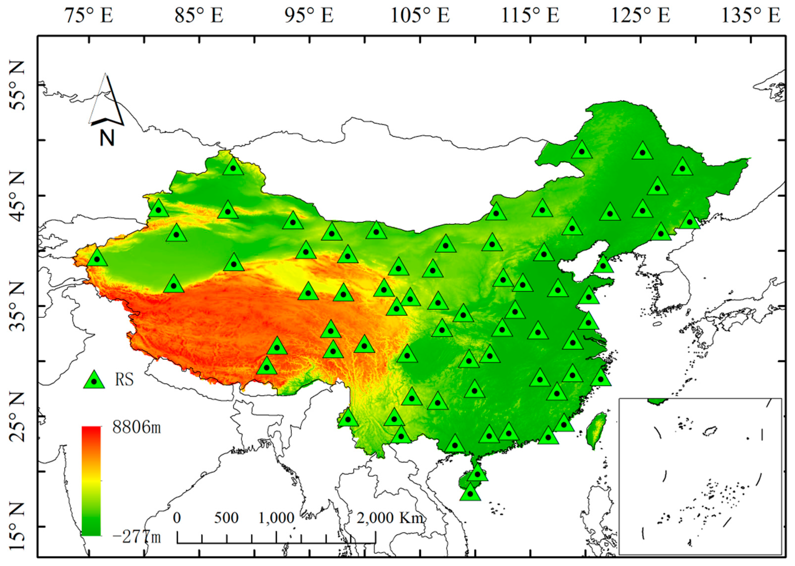
China has a vast territory with large undulations; high-altitude areas mostly occur in the Qinghai-Tibet Plateau and Yunnan-Guizhou Plateau. However, sounding stations are scarce and unevenly distributed in high-altitude areas, so building a high-precision Tm model on a large-scale using radiosonde data in high-altitude areas is challenging. Compared to the DEM in China, the maximum elevation difference in the study area is more than 6~8 km, which is suitable for the study of the elevation direction modeling of Tm. The distribution of the study area is shown in Figure 1.
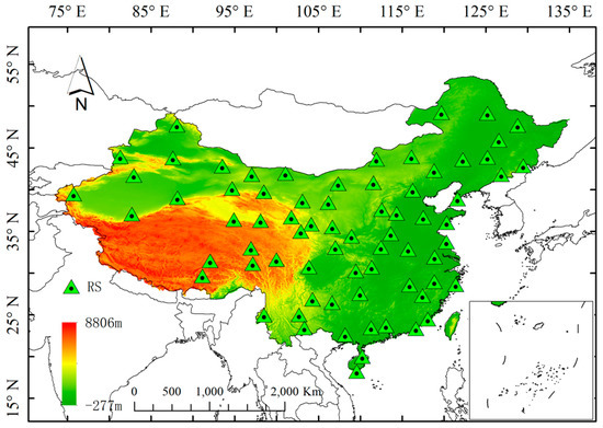
Figure 1.
The distribution of the study area and the radiosonde stations (RS) used for modeling.
Therefore, we selected 55~15° N and 70~140° E, including all of China as the research area. The pressure stratification data provided by ECMWF were used to construct a Tm model (CTm-h) in China with a nonlinear elevation correction. In addition, the common model usually obtains the Tm value of the ground surface, but because a height difference exists between the reference altitude plane of Tm and the GNSS site, this height difference often cannot be ignored when estimating Tm [18]. Therefore, we used the 1000–250 hpa (elevation 0–10 km) pressure layer as the bottom layer to integrate upwards to obtain the Tm at different heights, and modeled the vertical direction of Tm.
2.2. Research Data
Using the 2014–2018 reanalysis data in the ERA5 dataset provided by ECMWF, the original spatial resolution was 0.25° × 0.25°, the time resolution was 1 h, and the vertical resolution was 37 layers. To reduce the amount of data processing as much as possible without affecting the performance of the model, we selected the data of the four periods of 00:00, 06:00, 12:00, and 18:00 to simulate the changes in the day and night y, and downsampled the spatial resolution to 0.5° × 0.5°. Each layer of meteorological data includes temperature T (K), geopotential Z (m2/s2), specific humidity q (kg/kg), and air pressure P (hpa), which were used to calculate the Tm for all research grid points in China. Tm is calculated by the numerical integration method [4]:
A height difference often exists between the reference height level of the Tm model and the GNSS site. It is necessary to reasonably interpolate or extrapolate the Tm value obtained from the reference plane to the height of the GNSS site. This requires the lapse rate of Tm. Therefore, the lapse rate of Tm affects the precision of the final estimation of Tm [16,17,18,21]:
In Equation (2), T is the absolute temperature; β is the temperature lapse rate; h0 and are the height at the reference height and Tm, respectively; the range h − h0 is the entire troposphere; and Z is the height along the zenith direction. The water vapor pressure cannot be obtained through actual measurement; it needs to be calculated by [10]:
In Equation (3), Q is the specific humidity and P is the atmospheric pressure. Since ECMWF use geopotential height, they record different isobaric surfaces. GNSS stations and DEM elevations often use the WGS-84 coordinate system. Therefore, in terms of elevation transformation, it is necessary to convert its geopotential height to earth height [8].
3. Establishment of Tm Model (CTm-h) with Nonlinear Elevation Correction
3.1. Problems with Existing Tm Models
The current common Tm model usually chooses a linear function model for the correction in the elevation direction, and the expression is shown in Equation (4). At present, the commonly used method of calculating β is to substitute the Tm and height h of each pressure layer at a certain time into Equation (4) and obtain the Tm lapse rate β of the grid point at the corresponding time through the LSQ. The Tm lapse rate obtained by the linear function model is suitable for elevation correction in most low-latitude areas, and can achieve accurate results:
In Equation (4), β is the lapse rate of Tm (K/km), h is the height (km), and k is a constant.
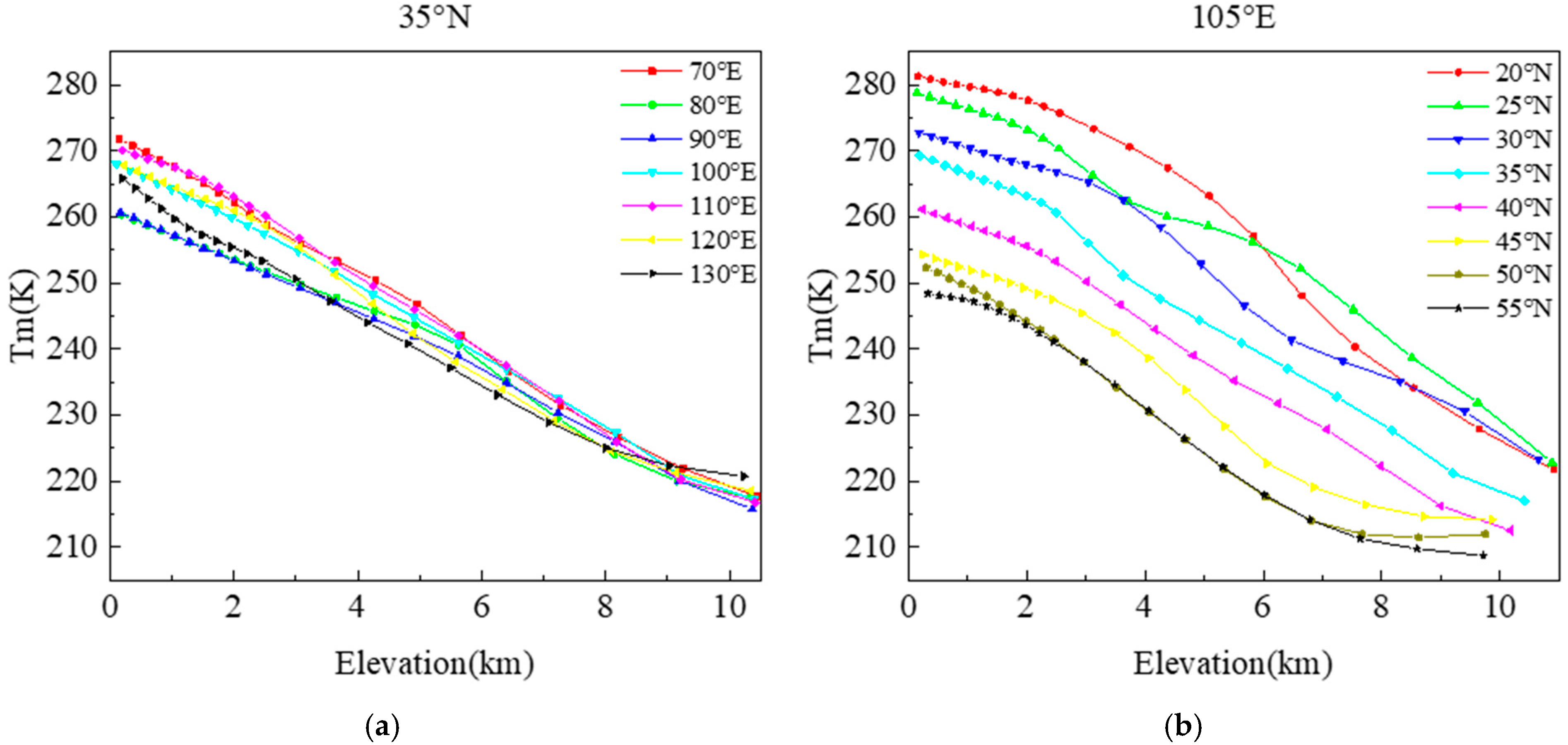
To analyze the change in Tm with elevation in the study area, several grid points, such as 35° N and 105° E area, were used to analyze the influence of longitude and latitude on Tm with elevation. The result is shown in Figure 2.
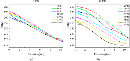
Figure 2.
Tm profile of 35° N (a) and 105° E (b).
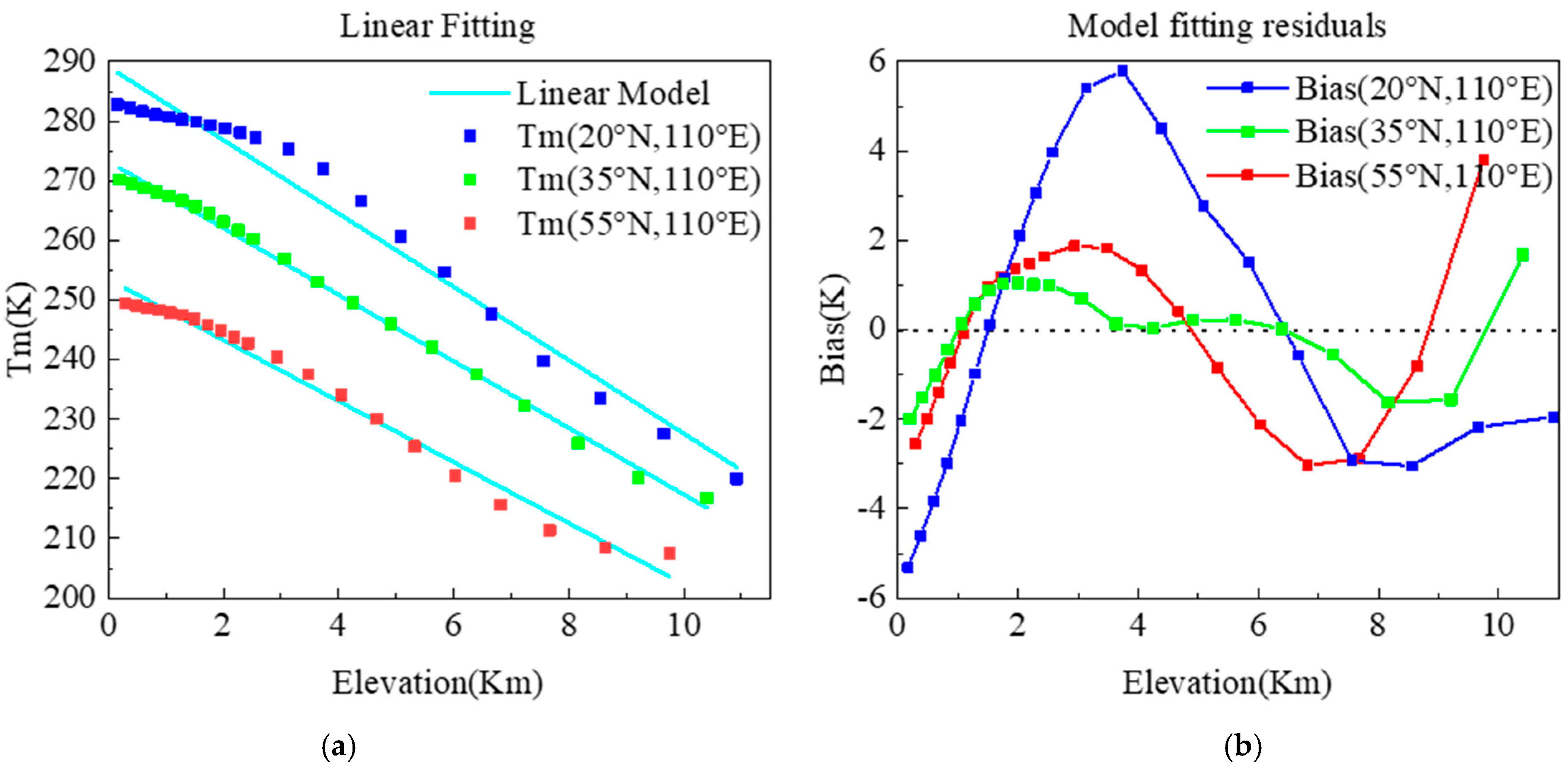
Figure 2a shows that the trend of the change in Tm for the grid points with different longitudes at the same latitude is not much different. However, as the latitude increases, Tm shows a clear downward trend (Figure 2b). In addition, the latitude changes in the Tm profile gradually show a trend of varying degrees of nonlinearity (Figure 2b). Specifically, the changes in the nonlinear characteristics of the Tm profile of some grid points in the study area with the height change are particularly consistent with the shape of the trigonometric function in mathematics. Nonlinear features do not necessarily appear in areas with higher latitudes, and similar situations occur for a large number of grid points at low latitudes. In this case, it is not appropriate to continue to use the linear function model (Equation (4)) to fit the Tm profile (Figure 3a), as it will affect the precision of the elevation correction (Figure 3b). Th linear function model is not the best solution in this case because it does not conform to the natural law of temperature changes with elevation. Regardless of low- or high-latitude regions, temperature changes with elevation show nonlinear characteristics, so it was necessary to establish a new model to obtain the characteristics of the Tm profile.
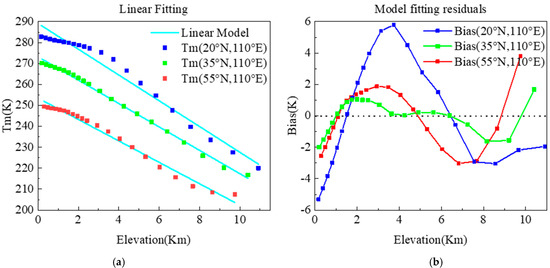
Figure 3.
Fitting effect of linear function model (a) and its residual (b).
3.2. Establishment of Tm Model with Nonlinear Elevation Correction (CTm-h)
As the linear function model does not fit the Tm profile well, we propose adding the Fourier function to the linear function model to fit the Tm profile. We consider it a model with a nonlinear elevation correction. That is, we use Equation (5) to fit the Tm profile:
In Equation (5), is the Tm value obtained by numerical integration for each pressure layer; α1, α2, α3, α4, and α5 are all the coefficients to be estimated, where α1 is the linear partial coefficient of Tm elevation correction, α2 and α4 are nonlinear partial coefficients, α3 is the coefficient related to the period of the Fourier function, and α5 is a constant. Enter the Tm and h of different heights from 0 to 10 km into Equation (5) and use the LSQ to solve for each coefficient. We used an equal weight strategy to estimate the model coefficients for the calculated Tm of each layer.
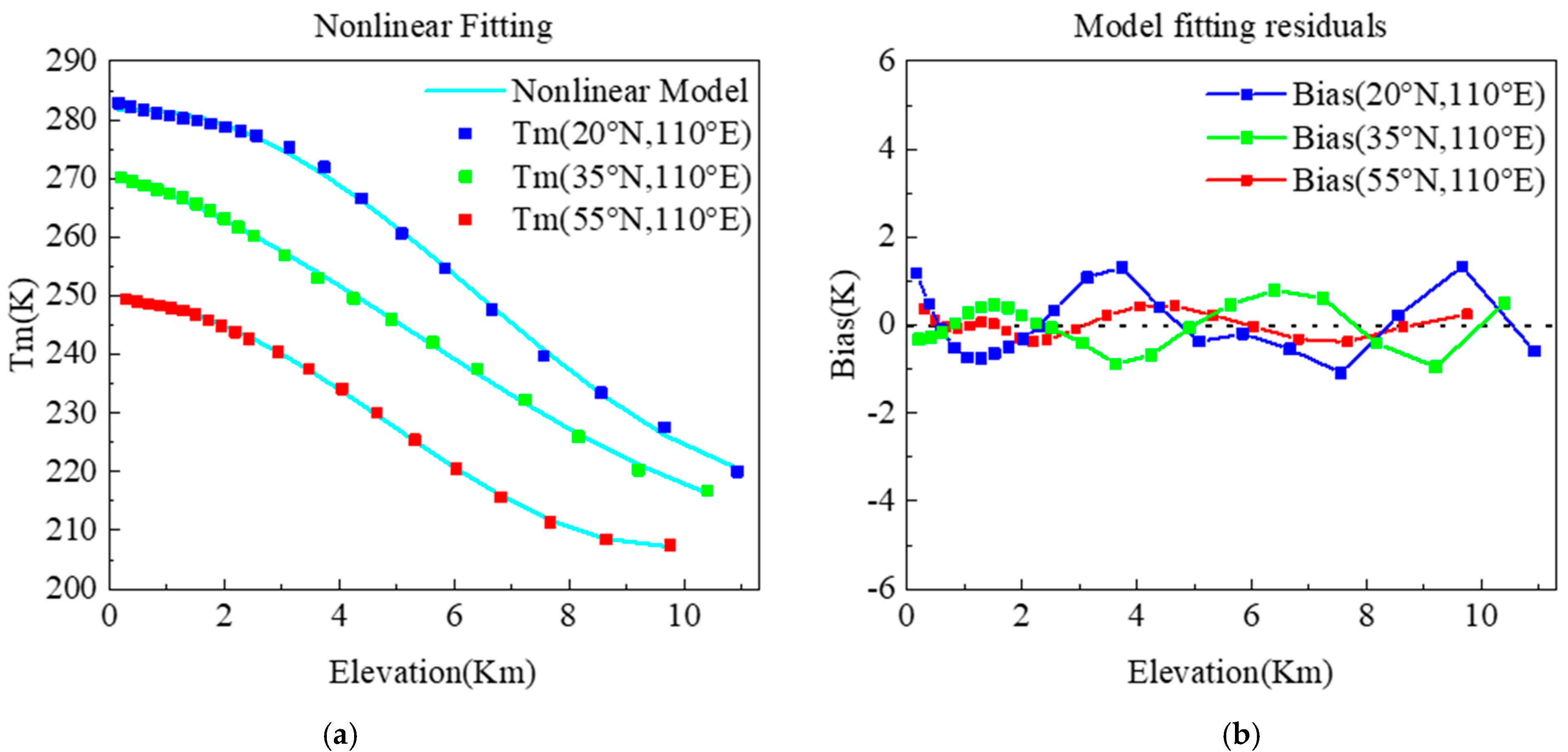
From the fitting result (Figure 4a) using Equation (5), the model with the nonlinear correction is more sensitive and effective in the elevation correction of Tm, which considerably reduces the error caused by the linear function model in the elevation direction (Figure 4b). We calculated the RMS of the two models. The RMS values of the linear function model (Equation (4)) and of the model with the nonlinear elevation correction (Equation (5)) are 2.69 K and 0.17 K, respectively. This means that Equation (5) accurately fits the change in Tm with elevation.
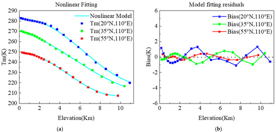
Figure 4.
Fitting results (a) and residuals (b) of the model with nonlinear elevation correction.
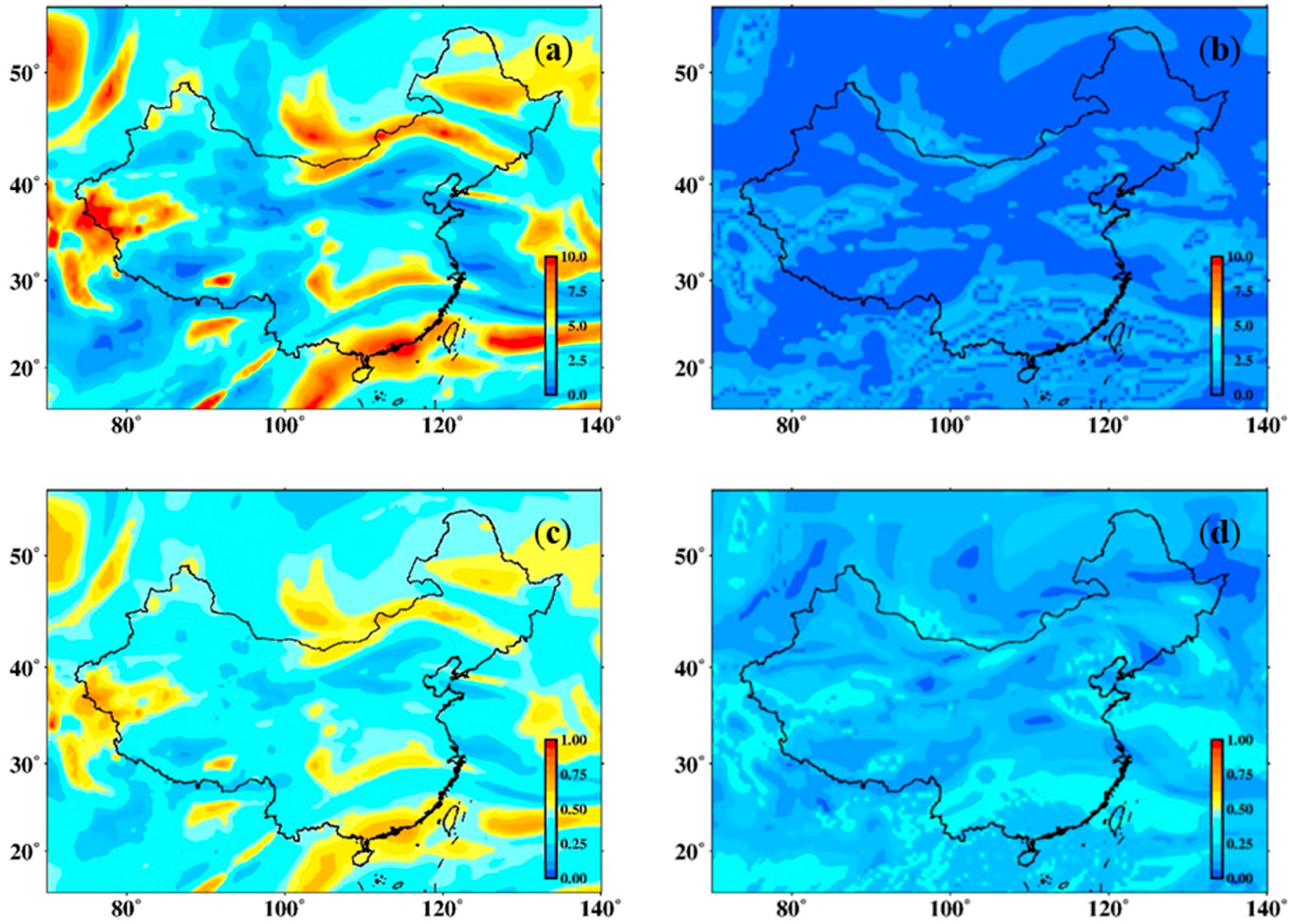
In addition, we used a linear function model (Equation (4)) and a model with a nonlinear elevation correction (Equation (5)) to fit the Tm profile of all grid points in the study area on 1 January 2018 and calculated the statistics (the average SD and RMS) of all grid points. The statistical results are shown in Figure 5.
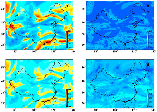
Figure 5.
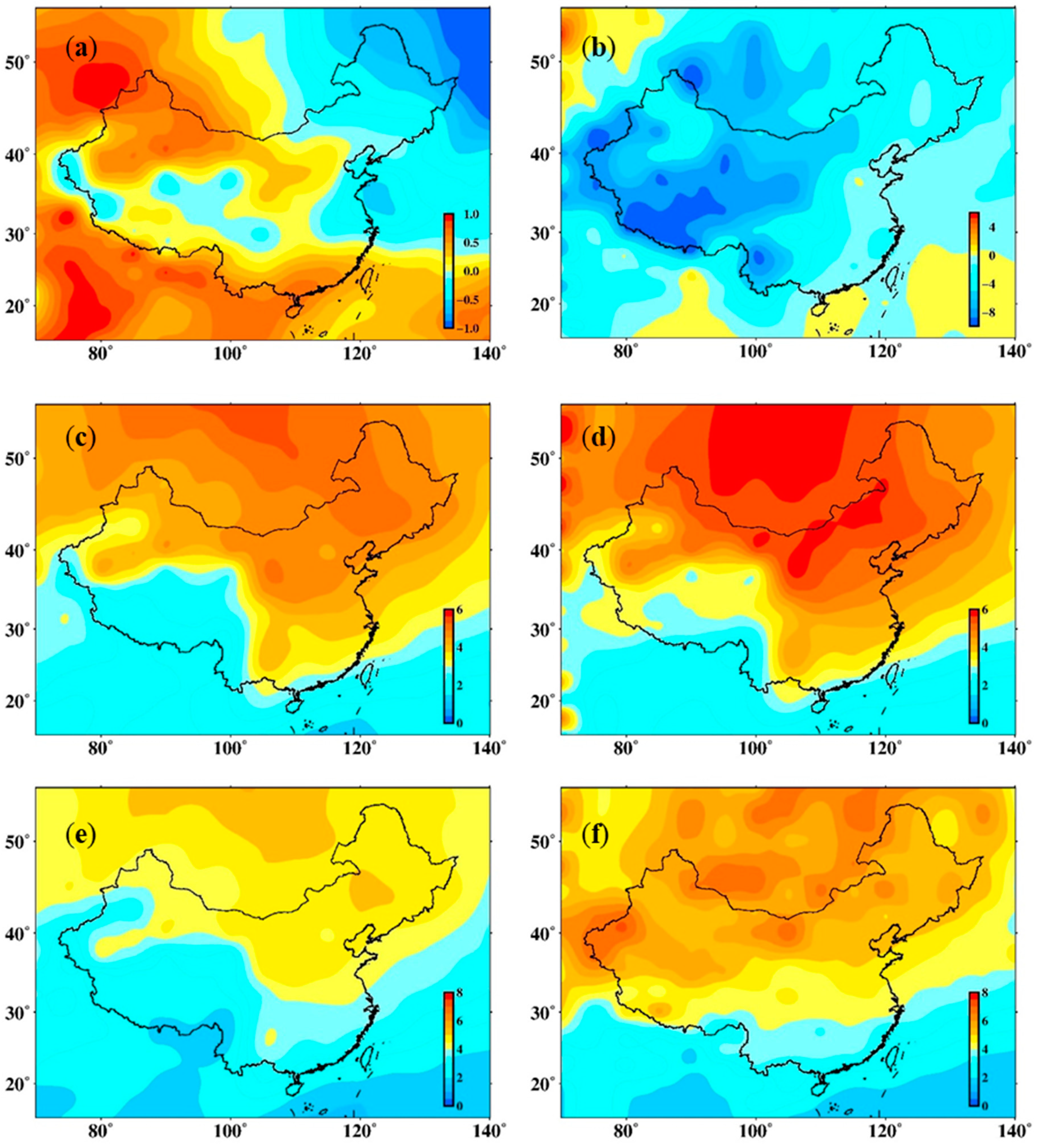
SD distribution (linear (a) and nonlinear (b)) and RMS distribution (linear (c) and nonlinear (d)) of all grid points in the study area.
The statistical results show that the average SD using the linear model is 4.84 K, and the average RMS is 0.48 K. The average SD using the model with the nonlinear elevation correction is 0.67 K, and the average RMS is 0.19 K. The SD of the linear model is much higher than that of the model with nonlinear elevation correction because the linear model does not well-fit the nonlinear trend in Tm with elevation changes, which leads to the discrete difference between the estimated value of the Tm obtained by the linear model and the calculated value. Figure 5a shows that in some areas, the maximum SD reached 9.6 K, which reflects that the stability of the linear function model is weak. This drawback was corrected after adding the nonlinear correction. The RMS of the model with the nonlinear elevation correction was improved by about 60% compared to the linear model, and higher precision was obtained on all grid points in the study area. This finding shows that although the study area (15~55° N) has middle and low latitudes, the change in Tm still has obvious nonlinear characteristics and cannot be ignored, proving that this nonlinear elevation correction is necessary and reasonable.
The pressure stratification data with a time resolution of 6h in the ERA5 data set provided by ECMWF were used. We calculated the time series of the model coefficients at four times (00:00, 06:00, 12:00, and 18:00 UTC) for the five years from 2014 to 2018. The time resolution of the data used in this paper is 6 h, which can indirectly reflect the changes in Tm to a certain degree.
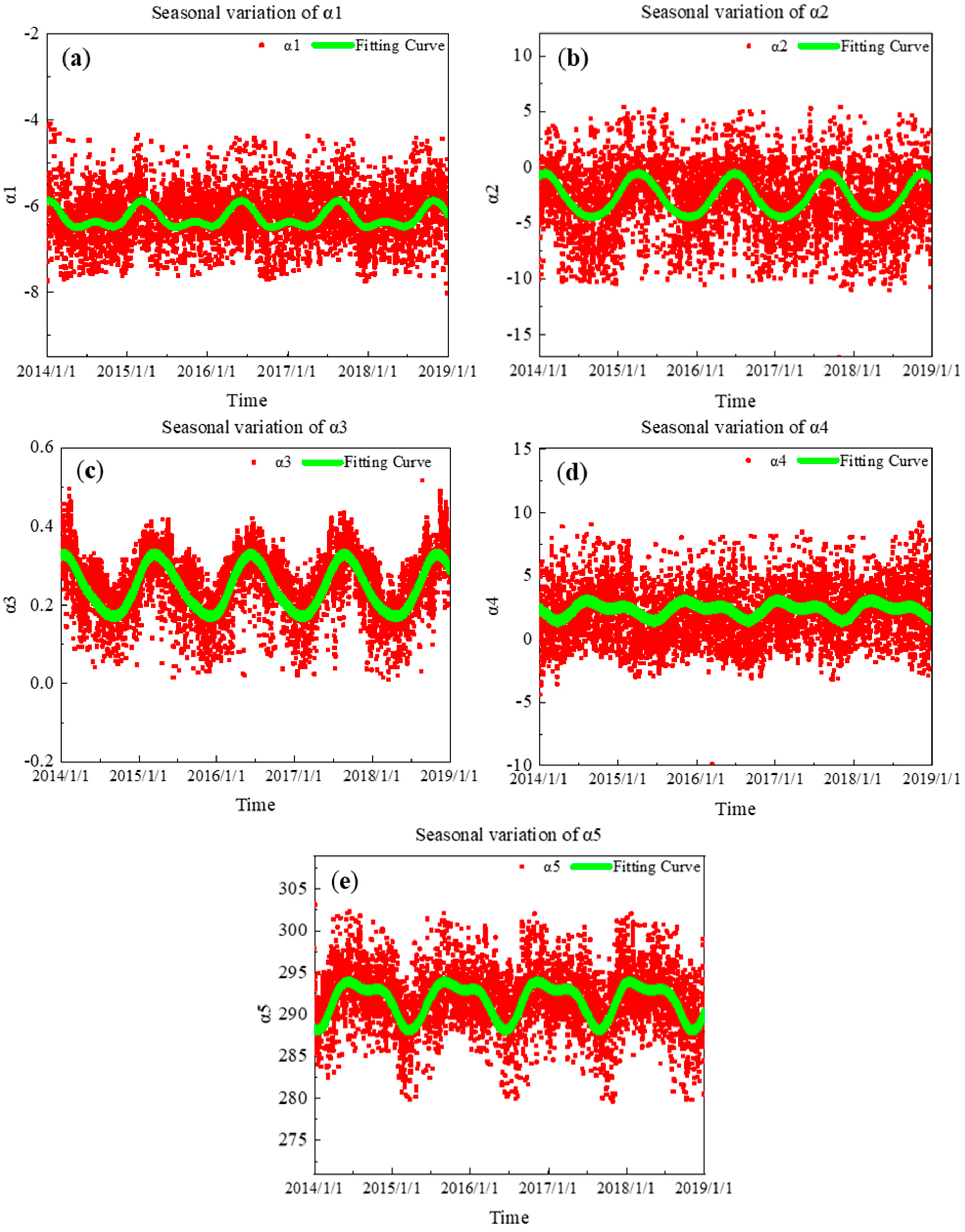
Therefore, firstly, we used Equation (5) to fit the changes of Tm in all pressure layers within 0~10 km at four times per day for 5 years. Secondly, the five coefficients of were fitted using Equation (6), which indirectly reflects the seasonal changes and daily changes in Tm. Figure 6 shows the fitting results of each model coefficient with grid points (55° N, 110° E) as an example:
where αi is the coefficient to be estimated, where the value range of i is 1~4; DOY is the day of the year; DOH is the hour of the day; and βj is the coefficient estimated by the least square principle, where the value range of j is 1~7.

Figure 6.
Time series of coefficients of the model with nonlinear elevation correction from 2014 to 2018 (α1 (a), α2 (b), α3 (c), α4 (d), α5 (e)): 55° N, 110° E.
When the proposed Tm model uses the LSQ for adjustment, since α3 is within the trigonometric function included in the Fourier function, the entire Equation needs to be linearized. Therefore, in the adjustment process, the strategy proposed by Yao et al. [19] is used, that is, α3 = π/10. This obtains a more accurate initial value of the coefficient in Equation (5), and then LSQ is used to adjust Equation (5).
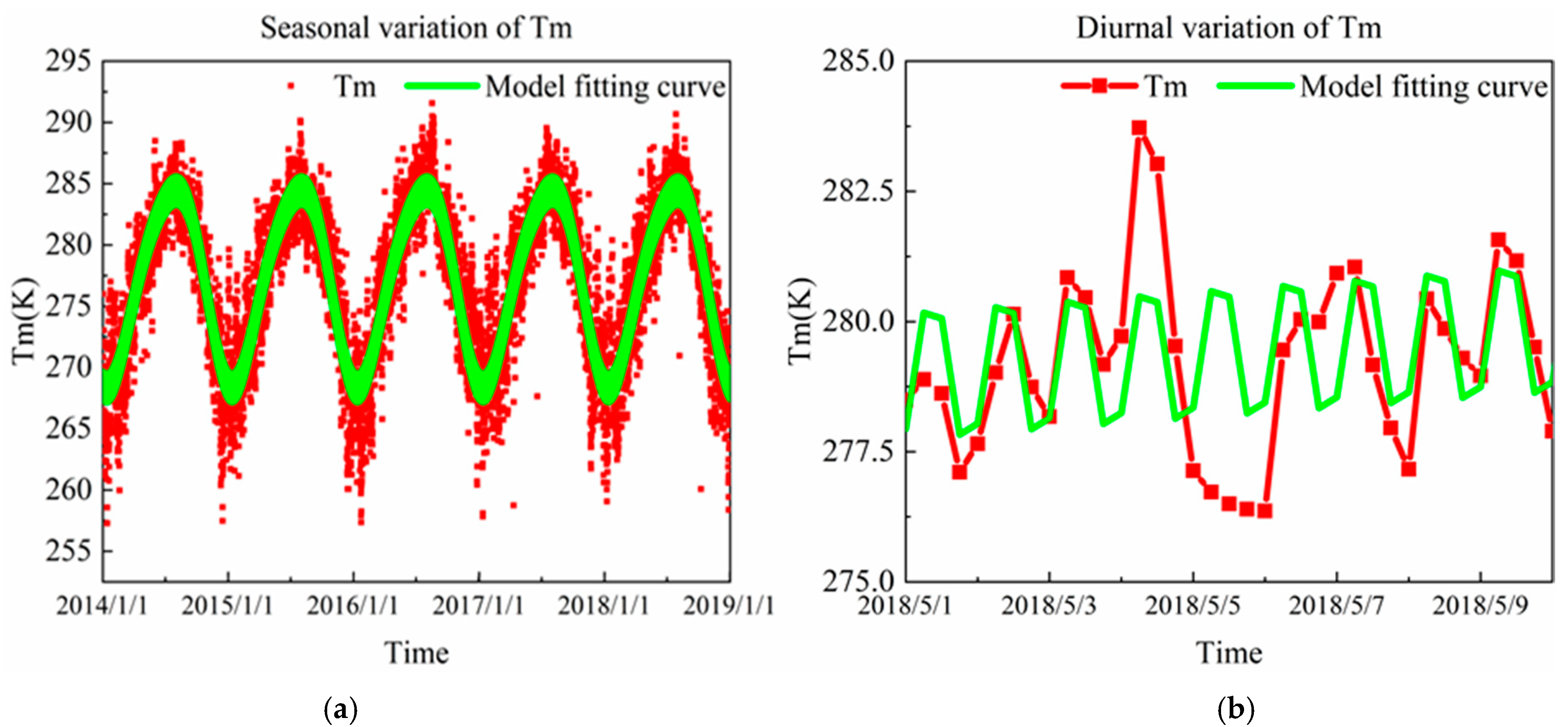
The Tm model with nonlinear elevation correction not only effectively fits the Tm in the elevation direction, but also increases the sensitivity and effectiveness of the correction of Tm. The spatial resolution of 0.5° × 0.5° effectively reduces the influence of latitude and other factors on Tm in the horizontal direction. Simultaneously, the model also considers the seasonal cycle and day–night variation of Tm, which ensures the precision of Tm remains high in the time series. We call the new model CTm-h. The fitting results are shown in Figure 7. Regardless of seasonal changes or daily changes, the Tm is well-reflected in the CTm-h model, with higher precision than provided by previous models.
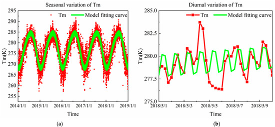
Figure 7.
Seasonal (a) and diurnal (b) changes in the values estimated by the model.
Notably, the CTm-h model is a grid empirical model. Using the ECMWF air pressure stratified data from 2014 to 2018, Equation (5) is first used to fit the Tm profile in the elevation direction of the grid points, and then Equation (6) is used to fit the model coefficients of the Tm profile of each grid point. The method used to solve the coefficients is the least square method, and the coefficients obtained are stored in the horizontal grid points with a resolution of 0.5° × 0.5°.
4. Results
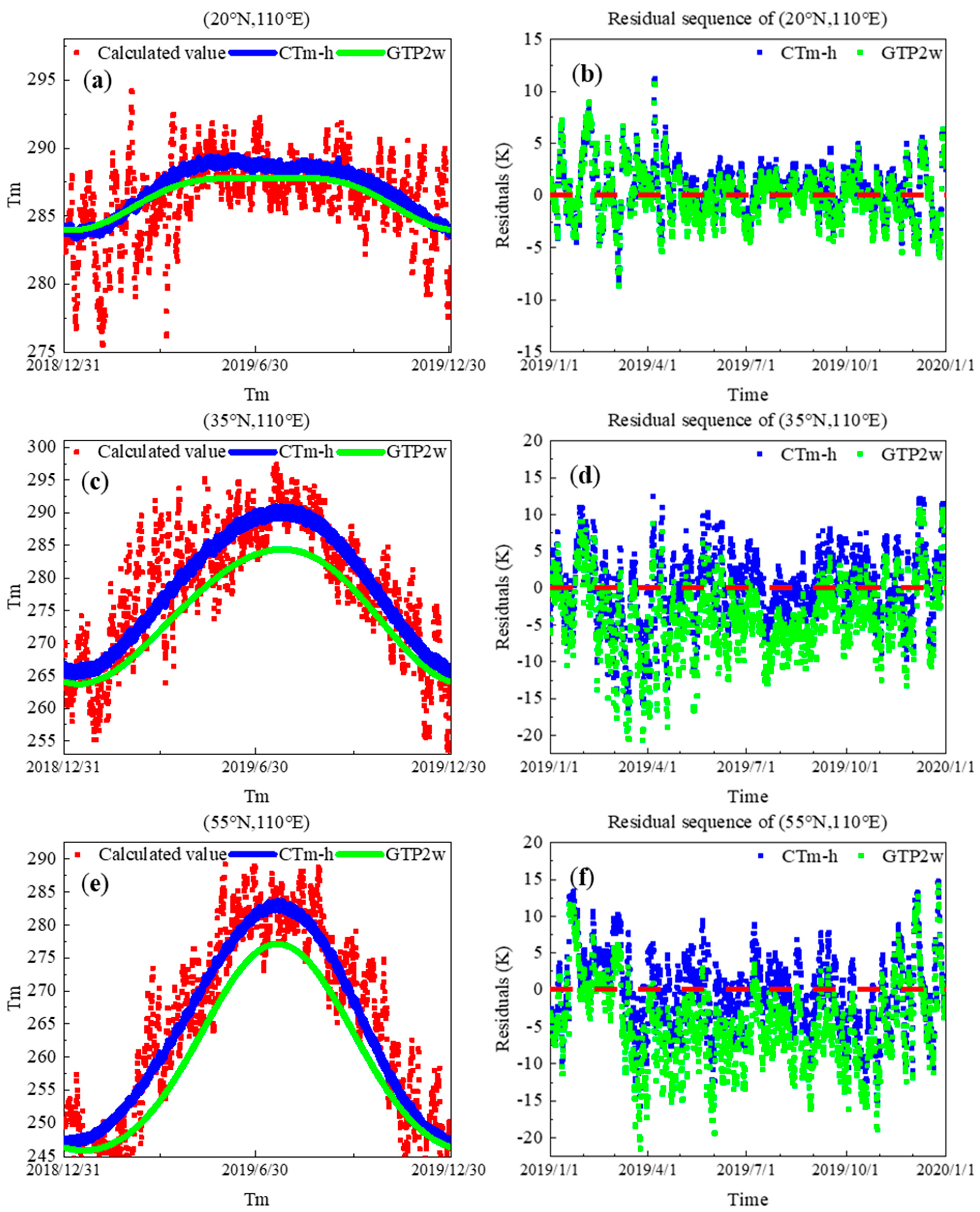
We used bias, RMS, and SD to evaluate model reliability. The ECMWF reanalysis data in 2019 that were not involved in the modeling were used to verify the precision of all grid points in the study area (55~15° N, 70~140° E). For related expressions, see Equations (5) and (6). First, we selected three grid points distributed in different latitudes in the study area, namely 20° N, 110° E; 35° N, 110° E; and 55° N, 110° E. We selected these three grid points at different latitudes as examples to evaluate the precision of the model. The precision of the CTm-h model was studied with the data from 2019 and the results were compared to those the GPT2w model, as shown in Figure 8. It is worth noting that although GPT3 is the latest version of the GPT series model, Tm has not been improved in GPT3. Therefore, the Tm in GPT3 still maintains the performance of GTP2w.
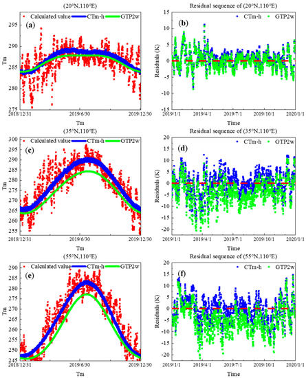
Figure 8.
Fitting results (a,c,e) and model residuals (b,d,f) (20° N, 110° E); (35° N, 110° E); and (55° N, 110° E).
Three grid points of different latitudes roughly located in the center of the study area were selected to study the precision of the CTm-h model, which was compared to the GPT2w model. Figure 8 shows that the model residuals of the CTm-h model at the three grid points are all around zero. From the perspective of residual distribution, the residual distribution of grid points at low latitudes (20° N, 110° E) is mostly concentrated in the (−5, 5) interval. The residual distributions for the other two grid points are roughly the same, most of which are in the (−10,10) interval. The residual error distribution of the GPT2w model at the 20° N, 110° E grid point is also concentrated in the (−5, 5) interval, which is equivalent to CTm-h. However, the residuals for the other two grid points show obvious negative deviations. The bias, SD, and RMS of the two models for the three grid points were calculated and compared. As shown in Table 1, the precision of grid points at low latitudes is higher than at mid-latitude regions. This is also a problem that occurs in the current Tm model and needs to be further analyzed. The precision of the three grid points (20° N, 110° E; 35° N, 110° E; 55° N, 110° E) is improved by 5%, 13%, and 22% compared to GPT2w, respectively.

Table 1.
Precision comparison of three grid points between CTm-h and GPT2w (K).
Then, the estimated and calculated values of Tm of all grid points in the study area were compared, and the distribution diagrams of bias, SD, and RMS of all grid points are depicted in Figure 9. Figure 9 shows that the average bias of the CTm-h model is positive in the west of the study area, and gradually decreases from west to east. The average bias of the CTm-h model in the entire study area is (−1,1), and most of them are near zero in China; GPT2w has a relatively obvious negative deviation in the northwestern region of China, and the overall average bias is in the (−8,4) interval. The RMS and SD of the two models both show an increase with increasing latitude, and their distributions are roughly the same. The model precision of the two models in the study area was calculated and is reported in Table 2. The average bias of the CTm-h model in China is 0.18 K, the average RMS is 3.43 K, the maximum RMS is 5.45 K, the average SD is 3.39K, and the maximum SD is 5.47 K. The average bias of the GPT2w model in for all of China is −2.48 K, the average RMS is 4.69 K, the maximum RMS is 6.68 K, the average SD is 3.58 K, and the maximum SD is 5.86 K.

Figure 9.
The average bias (a), SD (c), and RMS (e) distribution of CTm-h; the average bias (b), SD (d), an RMS (f) distribution of GPT2w.

Table 2.
Precision statistics of CTm-h and GPT2w models (K).
In terms of the overall situation, the precision of CTm-h in China has increased by about 26.8% compared to that of GPT2w, and higher precision can be obtained for the entire study area. Finally, we used the radiosonde data provided by IGRA to verify the precision of the CTm-h model. The official website of IGRA provides the data of a total of 218 radiosonde stations in China. However, some of the stations provide data that are not updated in real-time and the quality is poor. Therefore, we selected 71 radiosonde stations with sufficient high-quality data, uniformly distributed in China. Their distribution is shown in Figure 1. We calculated the average bias, RMS, and SD of each sounding station in 2019, and the results are shown in Figure 10.

Figure 10.
The average bias (a), SD (b), and RMS (c) of the CTm-h model verified by the radiosonde stations.
Figure 10 shows that from the verification using sounding data, the CTm-h model has a certain positive deviation in the study area. The average bias is positive throughout the study area, and gradually decreases from north to south. The bias at most sites is concentrated near 3 K. The SD and RMS also appear to rise with the increase in latitude, and the distribution is roughly the same. We calculated the average bias, SD, and RMS of the data from all sounding stations in the study area. From Table 3, the average bias of the CTm-h model verified by radiosonde data in China is 3.63 K, the average RMS is 4.64 K, the maximum RMS is 7.12 K, the average SD is 3.65K, and the maximum SD is 6.22 K.

Table 3.
Precision statistics of CTm-h model of radiosonde station (K).
5. Conclusions
In this study, ECMWF reanalysis data were used to analyze the distribution characteristics of Tm in the elevation direction in China. We found that Tm exhibits nonlinear changes in the vertical direction. Especially as the latitude increases, this nonlinear characteristic becomes more obvious. In response to this problem, we proposed using a combination of linear and Fourier functions to simulate the Tm profile. Then, based on LSQ fitting of the changes in the coefficient time series, a China Tm (CTm-h) model with a nonlinear elevation correction was established. We used ECMWF and radiosonde data to verify the precision of CTm-h. The results showed that when using ECMWF and radiosonde data, the RMS is 3.63 K and 4.64 K, respectively. Compared to the existing high-precision GPT2w model, the CTm-h model has higher precision by about 26.8%. This study shows that the CTm-h model can provide high-precision Tm estimates in China.
Author Contributions
All the authors participated in editing and reviewing the manuscript. G.H., H.Z. and K.C. conceived and designed the experiments; G.H. and H.Z. performed the experiments; G.H., H.Z. and K.C. analyzed and interpreted the results. All authors have read and agreed to the published version of the manuscript.
Funding
This research was funded by the Young Talent Promotion Project of China Association for Science and Technology, the National Natural Science Foundation of China (grant no. 42074024), The National Natural Science Foundation of China (nos. 41731066 and 41774025), The National Key Research and Development Program of China (no. 2018YFC1505102), The Outstanding Youth Foundation of Shaanxi (no. 2019JC-20), The Grand Projects of the BeiDou-2 System (no. GFZX0301040308), and The Special Fund for Basic Scientific Research of Central Colleges (no. CHD300102268305).
Institutional Review Board Statement
Not applicable.
Informed Consent Statement
Not applicable.
Data Availability Statement
The Radiosonde data prepared by IGRA are available at https://www1.ncdc.noaa.gov/pub/data/igra/ (accessed on 1 November 2020). The reanalysis data, consisting of ERA5 products, were released by ECMWF at https://www.ecmwf.int/ (accessed on 1 November 2020).
Acknowledgments
The author would like to thank the two anonymous reviewers for their valuable comments, the reanalysis data provided by ECMWF and the radiosonde data provided by IGRA.
Conflicts of Interest
The authors declare no conflict of interest.
References
- Barindelli, S.; Realini, E.; Venuti, G.; Fermi, A.; Gatti, A. Detection of water vapor time variations associated with heavy rain in northern Italy by geodetic and low-cost GNSS receivers. Earth Planets Space 2018, 70, 1–18. [Google Scholar] [CrossRef] [Green Version]
- Zhang, W.; Zhang, H.; Liang, H.; Lou, Y.; Cai, Y.; Cao, Y.; Zhou, Y.; Liu, W. On the suitability of ERA5 in hourly GPS precipitable water vapor retrieval over China. J. Geod. 2019, 93, 1897–1909. [Google Scholar] [CrossRef]
- Zhao, Q.; Yao, Y.; Yao, W.; Li, Z. Real-time precise point positioning-based zenith tropospheric delay for precipitation forecasting. Sci. Rep. 2018, 8, 7939. [Google Scholar] [CrossRef] [PubMed]
- Davis, J.L.; Herring, T.A.; Shapiro, I.I.; Rogers, A.; Elgered, G. Geodesy by radio interferometry: Effects of atmospheric modeling errors on estimates of baseline length. Radio Sci. 1985, 20, 1593–1607. [Google Scholar] [CrossRef]
- Bevis, M.; Businger, S.; Herring, T.A.; Rocken, C.; Anthes, R.A.; Ware, R.H. GPS meteorology: Remote sensing of atmospheric water vapor using the global positioning system. J. Geophys. Res. Atmos. 1992, 97, 15787–15801. [Google Scholar] [CrossRef]
- Li, L.; Wu, S.; Wang, X.; Tian, Y.; He, C.; Zhang, K. Seasonal Multifactor Modelling of Weighted-Mean Temperature for Ground-Based GNSS Meteorology in Hunan, China. Adv. Meteorol. 2017, 2017, 1–13. [Google Scholar] [CrossRef]
- Zhang, W.; Lou, Y.; Huang, J.; Liu, W. A refined regional empirical pressure and temperature model over China. Adv. Space Res. 2018, 62, 1065–1074. [Google Scholar] [CrossRef]
- Zhu, H.; Huang, G.; Zhang, J. A regional weighted mean temperature model that takes into account climate differences: Taking Shaanxi, China as an example. Acta Geod. Cartogr. Sin. 2021, 50, 356–367. [Google Scholar]
- Boehm, J.; Heinkelmann, R.; Schuh, H. Short Note: A global model of pressure and temperature for geodetic applications. J. Geod. 2007, 81, 679–683. [Google Scholar] [CrossRef]
- Lagler, K.; Schindelegger, M.; Bohm, J.; Krasna, H.; Nilsson, T. GPT2: Empirical slant delay model for radio space geodetic techniques. Geophys. Res. Lett. 2013, 40, 1069–1073. [Google Scholar] [CrossRef] [Green Version]
- Yao, Y.; Zhang, B.; Xu, C.; Yan, F. Improved one/multi-parameter models that consider seasonal and geographic variations for estimating weighted mean temperature in ground-based GPS meteorology. J. Geod. 2013, 88, 273–282. [Google Scholar] [CrossRef]
- Yao, Y.; Zhu, S.; Yue, S. A globally applicable, season-specific model for estimating the weighted mean temperature of the atmosphere. J. Geod. 2012, 86, 1125–1135. [Google Scholar] [CrossRef]
- Yao, Y.B.; Zhang, B.; Yue, S.Q.; Xu, C.Q.; Peng, W.F. Global empirical model for mapping zenith wet delays onto precipitable water. J. Geod. 2013, 87, 439–448. [Google Scholar] [CrossRef]
- Yao, Y.; Xu, C.; Zhang, B.; Cao, N. GTm-III: A new global empirical model for mapping zenith wet delays onto precipitable water vapour. Geophys. J. Int. 2014, 197, 202–212. [Google Scholar] [CrossRef] [Green Version]
- Böhm, J.; Möller, G.; Schindelegger, M.; Pain, G.; Weber, R. Development of an improved empirical model for slant delays in the troposphere (GPT2w). GPS Solut. 2014, 19, 433–441. [Google Scholar] [CrossRef] [Green Version]
- Yang, F.; Guo, J.; Meng, X.; Shi, J.; Xu, Y.; Zhang, D. Determination of Weighted Mean Temperature (Tm) Lapse Rate and Assessment of Its Impact on Tm Calculation. IEEE Access 2019, 7, 155028–155037. [Google Scholar] [CrossRef]
- Yang, F.; Guo, J.; Meng, X.; Shi, J.; Zhang, D.; Zhao, Y. An improved weighted mean temperature (Tm) model based on GPT2w with Tm lapse rate. GPS Solut. 2020, 24, 1–13. [Google Scholar] [CrossRef] [Green Version]
- Huang, L.; Peng, H.; Liu, L.; Li, C.; Kang, C.; Xie, S. An empirical atmospheric weighted mean temperature model considering the lapse rate function for China. Acta Geod. Cartogr. Sin. 2020, 49, 432–442. [Google Scholar]
- Yao, Y.; Sun, Z.; Xu, C.; Xu, X. Global Weighted Mean Temperature Model Considering Nonlinear Vertical Reduction. Geomat. Inf. Sci. Wuhan Univ. 2019, 44, 106–111. [Google Scholar]
- Mateus, P.; Catalão, J.; Mendes, V.B.; Nico, G. An ERA5-Based Hourly Global Pressure and Temperature (HGPT) Model. Remote Sens. 2020, 12, 1098. [Google Scholar] [CrossRef] [Green Version]
- Sun, Z.; Zhang, B.; Yao, Y. A Global Model for Estimating Tropospheric Delay and Weighted Mean Temperature Developed with Atmospheric Reanalysis Data from 1979 to 2017. Remote Sens. 2019, 11, 1893. [Google Scholar] [CrossRef] [Green Version]
Publisher’s Note: MDPI stays neutral with regard to jurisdictional claims in published maps and institutional affiliations. |
© 2021 by the authors. Licensee MDPI, Basel, Switzerland. This article is an open access article distributed under the terms and conditions of the Creative Commons Attribution (CC BY) license (https://creativecommons.org/licenses/by/4.0/).

