Abstract
Canopy closure (CC), a useful biophysical parameter for forest structure, is an important indicator of forest resource and biodiversity. Light Detection and Ranging (LiDAR) data has been widely studied recently for forest ecosystems to obtain the three-dimensional (3D) structure of the forests. The components of the Unmanned Aerial Vehicle LiDAR (UAV-LiDAR) are similar to those of the airborne LiDAR, but with higher pulse density, which reveals more detailed vertical structures. Hemispherical photography (HP) had proven to be an effective method for estimating CC, but it was still time-consuming and limited in large forests. Thus, we used UAV-LiDAR data with a canopy-height-model-based (CHM-based) method and a synthetic-hemispherical-photography-based (SHP-based) method to extract CC from a pure poplar plantation in this study. The performance of the CC extraction methods based on an angular viewpoint was validated by the results of HP. The results showed that the CHM-based method had a high accuracy in a 45° zenith angle range with a 0.5 m pixel size and a larger radius (i.e., k = 2; = 0.751, = 0.053), and the accuracy declined rapidly in zenith angles of 60° and 75° ( = 0.707, 0.490; = 0.053, 0.066). In addition, the CHM-based method showed an underestimate for leaf-off deciduous trees with low CC. The SHP-based method also had a high accuracy in a 45° zenith angle range, and its accuracy was stable in three zenith angle ranges (: 0.688, 0.674, 0.601 and = 0.059, 0.056, 0.058 for a 45°, 60° and 75° zenith angle range, respectively). There was a similar trend of CC change in HP and SHP results with the zenith angle range increase, but there was no significant change with the zenith angle range increase in the CHM-based method, which revealed that it was insensitive to the changes of angular CC compared to the SHP-based method. However, the accuracy of both methods showed differences in plantations with different ages, which had a slight underestimate for 8-year-old plantations and an overestimate for plantations with 17 and 20 years. Our research provided a reference for CC estimation from a point-based angular viewpoint and for monitoring the understory light conditions of plantations.
1. Introduction
Plantations, as a major component of forest ecosystems, play an important role in biodiversity conservation, climate change and economic development [1,2]. Poplar plantations provide a large amount of timber and forest products in China [3]. So, it is essential to investigate the resources of poplar plantation timely and accurately [4].
The canopy structure affects different species in forest ecosystems by affecting light levels [5]. Canopy closure (CC), as a useful biophysical parameter for forest canopy structure, is widely used as an index for carbon fluxes, forest production, biodiversity and ecosystem functions by affecting energy transmission and microclimate in forest ecosystems [6,7,8,9]. Jennings et al. (1999) defined CC as “the proportion of sky hemisphere obscured by vegetation when viewed from a single point” to distinguish it from the concept of canopy cover, which was defined as the “proportion of the forest floor covered by the vertical projection of the tree crowns” [10]. Although both parameters are related to the penetration of light though the canopy, CC includes all sizes of gaps in the field of view (FOV), while canopy cover focuses on the space between crown gaps [11]. From an ecological view, CC is more meaningful for understory light conditions, which can be used to estimate other canopy indices such as leaf area index (LAI) and foliage clumping index [12,13,14,15].
The filed measure of CC often used hemispherical photography (HP) and quantum sensors (e.g., LAI-2200) [16,17,18]. Compared to quantum sensors, HP has the advantage to record the geometry of canopy openings from different zenith angles with a permanent two-dimensional form [19,20], but it needs to be taken at dawn, dusk or under an overcast sky due to the influence of sky lighting [21]. Despite the proven feasibility of HP, it is still time-consuming in image acquisition and processing, thus limiting its application on a large scale.
Synthetic Aperture Radar (SAR) and Light Detection and Ranging (LiDAR) have been widely studied for forest ecosystems to quantify the three-dimensional (3D) vertical structure of the forests [22,23,24,25]. LiDAR is superior to SAR for reconstructing the 3D structure of the tree canopy more accurately and is less sensitive to different forest vegetation [26]. However, LiDAR has a penetrating ability, is less affected by solar illumination and is thus considered superior to passive optical sensors in CC extraction [27,28]. Airborne LiDAR data enable a large-scale continuous monitoring of the biophysical parameters in forest ecosystems, such as biomass, tree species, tree height and CC [29,30,31,32]. In the literature, the common form of CC extraction is to calculate the ratio of the canopy hits above a specified height threshold based on airborne LiDAR data, and the threshold performs well when using the height of HP acquisition [33,34]. Hopkinson and Chasmer (2009) also found that CC can be calculated based on the ratio of the LiDAR return intensity, and the results required little calibration [35]. Another similar way is using the ratio between the number of canopy pixels and the total pixels, which is based on the canopy height model (CHM) generated from LiDAR data. The height threshold of canopy separation often used a fixed value, like 2 m [28,36,37]. A circular analysis window is needed for modeling CC with CHM to delineate the field of view (FOV), and its radial distances are not very clear, often using a fixed value or the height of the forest canopy [35,38,39]. Another promising method is to convert the point cloud into the angular FOV directly, to correspond to the characteristics of the photographs. This method is based on synthetic hemispherical photographs (SHP) from LiDAR data. Many studies have proved that the SHP-based method is reliable in evaluating canopy indices and solar irradiance based on the terrestrial LiDAR [40,41,42] and airborne LiDAR [13,43,44,45].
Recently, an unmanned aerial vehicle (UAV) has become an alternative remote sensing platform, which can effectively monitor the forest parameters by carrying different sensors [46,47,48,49]. The UAV-RGB system (i.e., a UAV platform carrying a camera or sensor with red, green and blue bands), a widely used UAV system, is often used for forest classification and parameters extraction in combination with deep learning algorithms, because it can obtain ultra-high spatial resolution images to describe forest characteristics [50]. Meanwhile, image processing techniques, such as structure from motion (SfM), can be used to generate dense point clouds from RGB images to estimate forest parameters [51]. Although the UAV-RGB system has a lower cost, the UAV-LiDAR system has its advantages in monitoring the forest’s 3D structure due to its ability to penetrate the canopy [52]. Moreover, the UAV-LiDAR system has been proven to be more accurate than the airborne LiDAR system in forest parameter investigations because of its higher density point cloud, simple operation, flight flexibility and lower costs [52,53,54,55]. Brede et al. (2017) compared terrestrial LiDAR and UAV-LiDAR for estimating forest canopy heights and diameter at breast heights (DBH), and their results showed a strong correlation of two LiDAR data in the DBH estimation ( = 0.98) [56]. Liu et al. (2018) evaluated the capability of the UAV-LiDAR system for estimating forest structural attributes and analyzed the effects of point cloud densities. They found that it was robust for estimating forest attributes when the point cloud density is higher than 16 pts·m−2 [57]. Wu et al. (2019) used UAV-LiDAR data to estimate the canopy cover of a ginkgo-planted forest with three methods and found that the CHM-based method with a 0.5 m resolution had a high accuracy ( = 0.92) [54]. Thus, the UAV-LiDAR data with high density point cloud are highly advantageous in describing the forest canopy structure, which has a high potential for an accurate CC extraction.
Although there have been many studies using LiDAR data for CC extraction, few of them evaluate the method based on CHM and SHP comprehensively, such as exploring the effects of different FOVs on different methods and explaining the scope of applicability of different methods. Moreover, previous studies rarely focused on the CC estimation in forest plantations based on UAV-LiDAR data. Therefore, this study aims to evaluate an efficient method to extract CC directly from UAV-LiDAR data. To achieve this goal, the specific objectives are: (1) to estimate CC in three zenith angle ranges, of 45°, 60° and 75°, based on CHM and SHP data from UAV-LiDAR data; (2) to validate the results of the two CC extraction methods by the classification results from HP data; (3) to explore the effect of different resolutions and stand ages on CHM-based and SHP-based methods.
2. Materials and Methods
2.1. Study Area
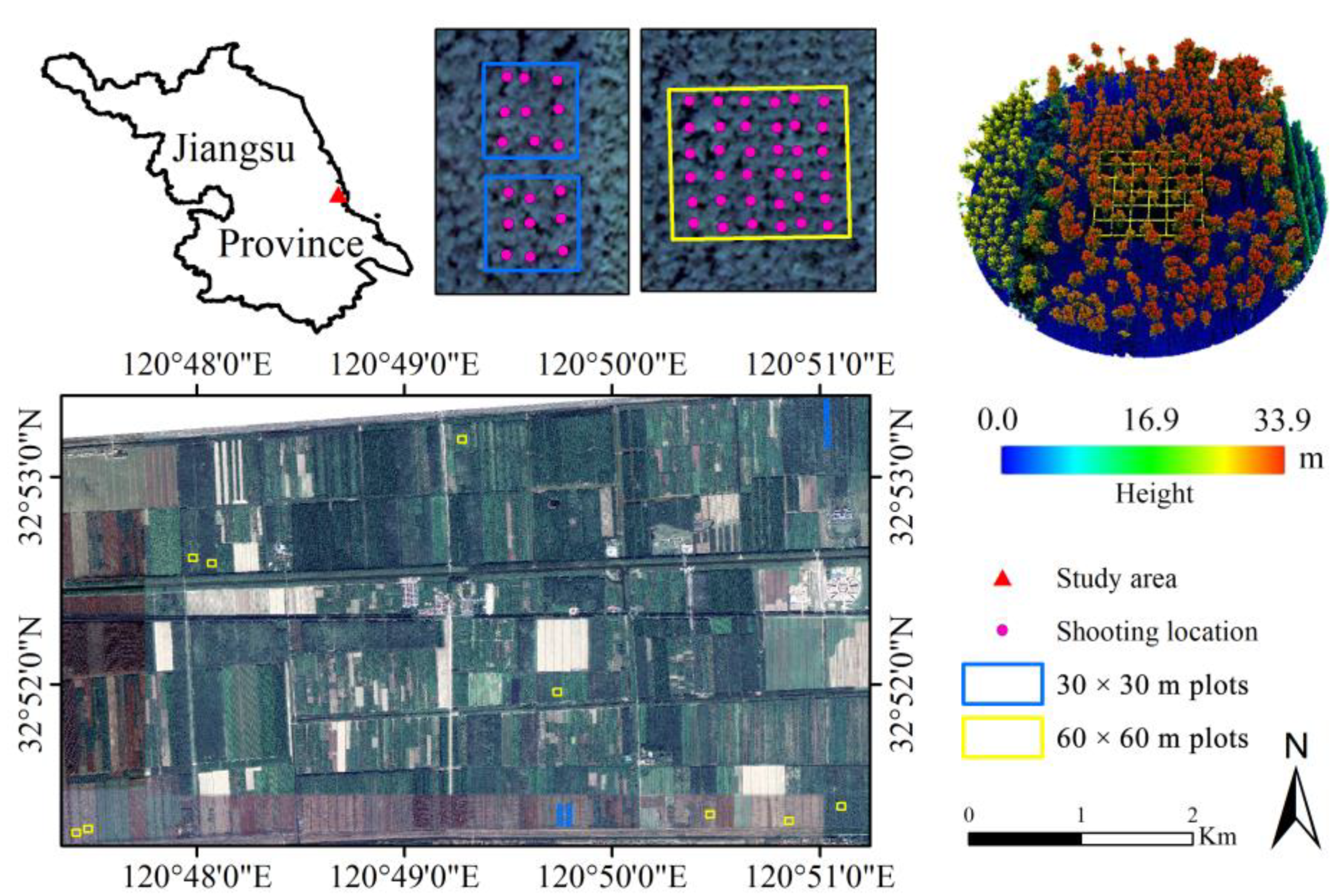
The study area is located in Dongtai City, Jiangsu Province (Figure 1). The area is flat, with a range of elevation from 11 to 14 m. It falls in the climate region of the transition zone between the subtropical and warm temperate area [58]. The annual mean temperature is 15.4 °C, the annual rainfall is 1494.0 mm and the average relative humidity is 76.0% [58]. The main soil type is desalted meadow soil, and the soil texture is sandy loam, alkaline (pH = 8.2). The main tree species include poplar (Populus deltoids), fir (Metasequoia glyptostroboides), ginkgo trees (Ginkgo biloba L.). Among all the three species, poplar has the largest plantation area, as well as with a variety of stand ages.

Figure 1.
The study area and field sample design. The pink dots are the location of the photos taken, the yellow and blue rectangular boxes represent two different size sample plots.
2.2. Field Design and Field Data Collection
The field work was conducted in May 2021. According to the difference in the size of poplar sublots, two different scale plots were set (60 × 60 m, 30 × 30 m; Figure 1). The plots contain varying stand ages, planting spacing and canopy structural characteristics (Table 1). A total of 29 square sample plots were measured, including 20 small plots (i.e., the total area is 900 m2) and 9 large plots (i.e., the total area is 3600 m2). Each of the plots was divided into several small blocks by a 10 × 10 m grid, and the center of each small block was the location for taking HP (Figure 1). In total, 570 HP were collected from 29 plots. All the HP were taken horizontally using a Canon M50 with a LAOWA CF 4 mm F2.8 circular fisheye lens. The camera was fixed on a tripod and each photo was taken 1.4 m above the ground. The HP was taken before sunrise, after sunrise or during daytime at an overcast sky to ensure a low light condition. All photos were taken in auto-exposure mode, and the shooting location was avoided too close to the trees. The shooting location was recorded below the tripod using a HUACE T10 real-time-kinematic (RTK) equipment (centimeter accuracy), and corrected with high precision real-time signals received from continuously operating reference stations (CORS). The recorded location of the global positioning system (GPS) points was regarded as the shooting location of HP.

Table 1.
The descriptions of poplar plot per site location.
The UAV-LiDAR data were collected via a Velodyne VLP-16 LiDAR sensor carried by a six-rotor DJI M600 PRO UAV. The parameters of the LiDAR sensor are as follows: wavelength 903 nm, vertical scanning angle ±15°, horizontal scanning angle 360° (a range of ±70° was reserved), pulse frequency 30 kHz. The flight parameters are the following: flight altitude 70 m, flight speed 3.6 m·s−1, flight interval 60 m. The point density of different sample plots was not the same because of the difference of flight strip numbers (Table 1). In addition, the forest planting spacing, the average tree height and the average branch height of each plot were collected for the subsequent data processing and analysis (Table 1).
2.3. Methodology
After the pre-processing of UAV-LiDAR data, including georeferencing, strip alignment, merging, de-noising and the interpolation of point clouds with different types, CHM and a normalized point cloud were generated. Then the shooting locations of HP data were used to delineate the FOV in CHM and normalized point cloud data, and the CC of different plots was extracted by height based on the FOV-CHM. SHP data were generated using a 3D polar coordinate conversion method to extract CC from all the normalized point cloud data directly. Finally, the CC extracted by the UAV-LiDAR data of different resolutions was validated by the results from HP data in different FOVs. The age effects of poplar plantations on CC extraction from UAV-LiDAR point cloud data were also explored in this study. In addition, a new classification model was developed to extract CC from HP data in this study as the validation data to compare the CC extraction result from UAV-LiDAR point cloud data using the CHM-based and SHP-based methods. An overview of the flowchart for CC extraction is shown in Figure 2.
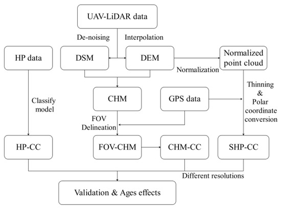
Figure 2.
Methodology flowchart. DEM: digital elevation model; DSM: digital surface model; CHM: canopy height model; HP: hemispherical photography; FOV: field of view; SHP: synthetic hemispherical photography; CC: canopy closure.
2.3.1. Preprocessing of UAV-LiDAR Point Cloud Data
The raw UAV-LiDAR point cloud coordinate was transformed based on UAV station GPS data, inertial measurement unit (IMU) data and base station data. Each strip was adjusted by a surface matching method based on the iterative closest point (ICP) algorithm [59]. After merging all the strips, the noised points were removed depending on the maximum distance from the point to its neighboring points in the LiDAR360 software. The ground points were classified by an improved progressive triangulated irregular network (TIN) densification filtering algorithm [60]. Then, the ground points were interpolated to generate the digital elevation model (DEM) by the TIN algorithm, and the digital surface model (DSM) was generated by the same interpolation method. Then, we subtracted the DEM from the DSM to generate CHM of different resolutions. We also normalized the height of the denoising point cloud based on the DEM to generate normalized point cloud data in preparation for the subsequent generation of SHP data.
2.3.2. Preprocessing of HP and FOV Delineation
Each photo was checked for quality, and the ones with overexposure and underexposure were discarded. We cropped all the photos and reduced the effect of image local highlights in the Adobe Photoshop CC 2019 software. The resolution of the processed photo was 3124 × 3124 pixels. The directed upward HP had a nearly polar projection, so the azimuth angle and zenith angle ranges of the photo could be divided according to the center of the photo [20]. Considering the difference of CC extraction results in different zenith angle ranges [42,61], we calculated the CC from three zenith angle ranges, of 45°, 60° and 75°. The different zenith angle ranges represented the different FOVs and radius in the image (Equation (1)).
where is the radius of the entire FOV in the photograph, and 90° represents the theoretical maximum zenith angle. is the zenith angle, which in this study is 45°, 60° and 75°. is the new radius with different FOVs in HP.
2.3.3. CC Extraction by the CHM-Based Method with a Hemispherical FOV
Compared to the estimation of canopy cover using CHM, it is a challenge to estimate the CC using CHM by a hemispherical FOV. In this study, the delineated FOV was used as the analysis window to calculate CC based on the CHM data generated by the preprocessed point cloud data. Because the FOV for field measured CC has the shape of an inverted cone, the horizontal radius of the analysis window should be generated based on the tree height [38]. However, the analysis window radius in the CHM-based method was not clear in previous studies [35,62]. Parent et al. (2014) put it forward using the height multiplied by the tangent of the zenith as the CHM radius range [37], but we found the radius of this model too large to fit the actual results of HP data in our study. Thus, we improved this FOV-delineated model based on the average height of the sample plot and the zenith angle of interest (Equation (2)).
where is the radius of the CHM analysis window; is the distance coefficient to adjust the radius (i.e., the radius that with is 2 and 3 in the three zenith angle ranges); is the average height of a sample plot, and is the zenith angle of interest.
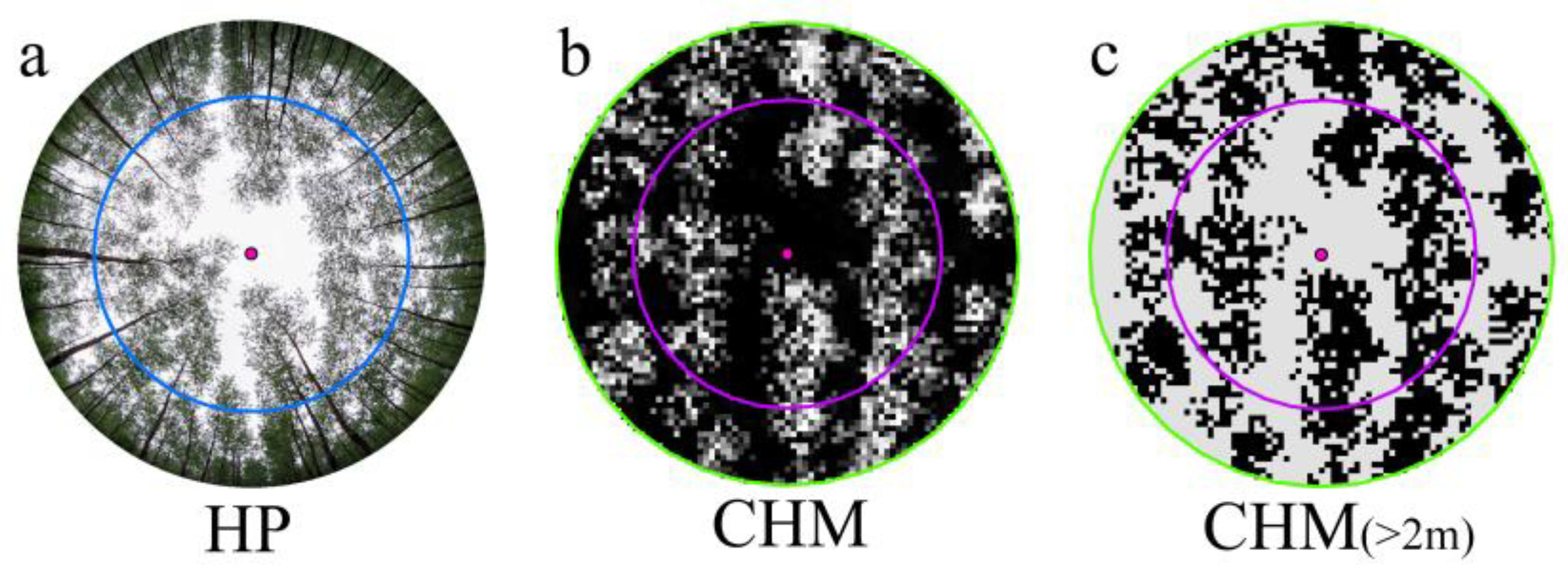
CC extraction from CHM images is a method based on the ratio of extracted canopy pixels to total pixels. The separation of canopy pixels and non-canopy pixels usually used a fixed height threshold (i.e., 2 or 3 m [28]). By using this threshold, the point cloud of the low plants had little effect on the generation of CHM data, so a CHM image with a height greater than this threshold is assumed as canopy pixels (Figure 3). However, the spatial resolution of CHM images might have influences on CC extraction. Thus, it is worth to explore whether there is an optimum spatial resolution to extract CC with the CHM-based model. Thus, we generated CHM with three spatial resolution, of 0.5, 2 and 5 m, for a sensitivity analysis. The CHM images were generated by a preprocessed point cloud data, and the different spatial resolutions were generated through an interpolation algorithm (see the description in Section 2.3.1). All the steps of the CHM-based method were written as a python script (see Supplementary Materials) to enhance the capacity of automatic batch-processing of this method.
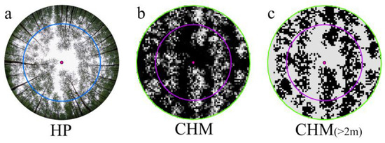
Figure 3.
Examples of CHM-based method. (a) a sample of HP: the pink dot is the view point of HP, and the blue circle is the zenith angle of 60° in HP.; (b) CHM image with a spatial resolution of 0.5 m generated from the UAV-LiDAR point cloud data collected in the same location of (a): the green circle and the purple circle represent the analysis window range when is 2 and 3, respectively; (c) a height threshold of 2 m was applied to (b): the black and grey pixels in (c) are canopy pixels and non-canopy pixels, respectively.
2.3.4. Estimation of CC with a SHP-Based Method
In order to extract CC from a point-based angular viewpoint, we transformed the coordinate system of the normalized point cloud data. The traditional Cartesian coordinates (x, y, z) were converted into polar coordinates (, , ), and all the point cloud data were printed in the polar coordinate system to simulate the photos taken by a circular fisheye lens [44] (Equation (3)).
where is the zenith angle in the polar coordination; is the azimuth in the polar coordination; is the distance between point cloud and the shooting location; are the 3D properties of the point cloud; are the GPS-coordinates of the shooting location; is the height of the camera set (a constant of 1.4 m in this study).
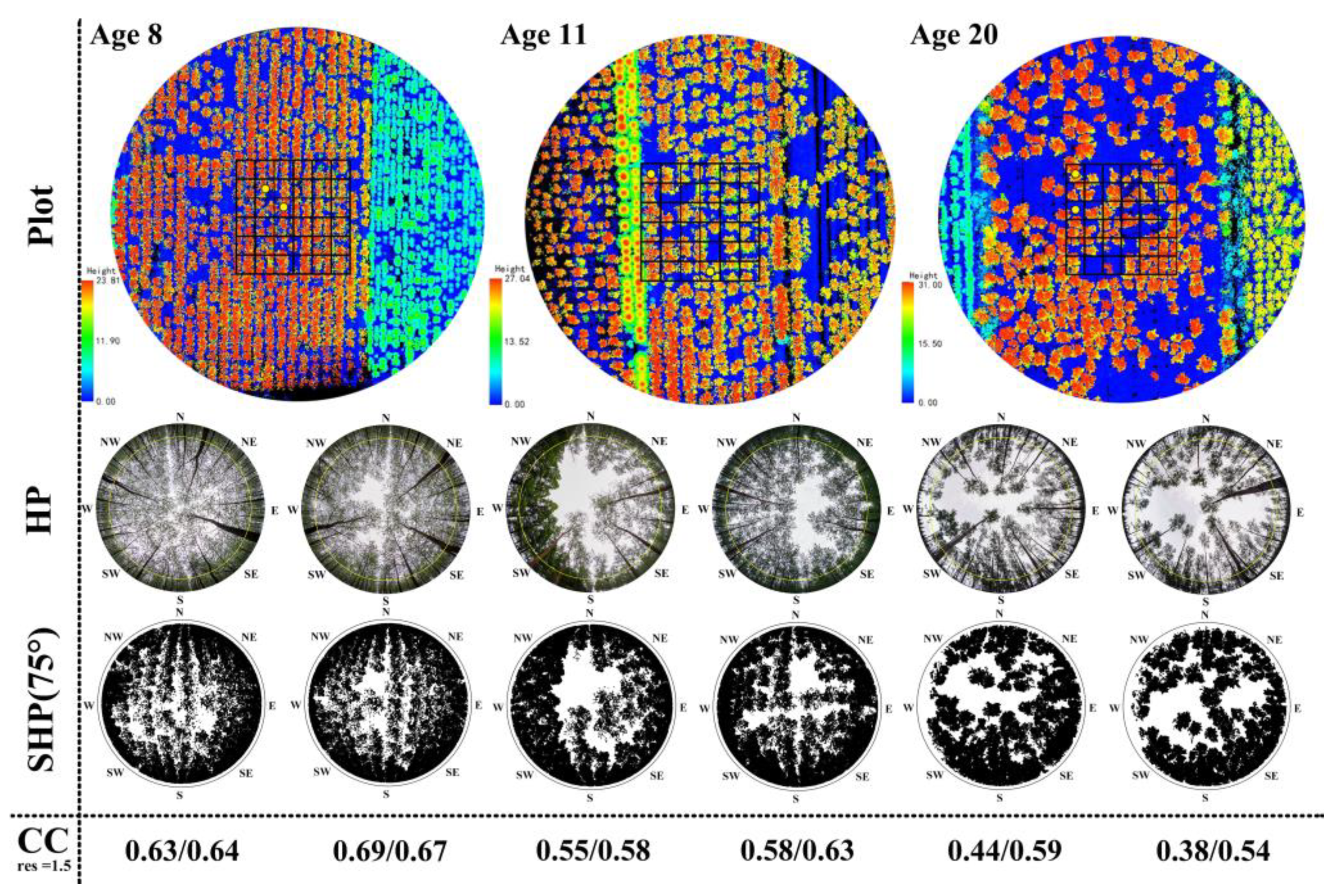
The maximum horizontal distance between the transformed point cloud and origin (i.e., shooting location) would have an effect on the results [44]. A large distance would ensure the correctness of the results [44], but the huge data of the point cloud would reduce the efficiency of the computing process. Considering that the maximum zenith angle in our study was 75°, we used the maximum tree height multiplied by a tangent of 75° as a theoretical distance range of the point cloud data in this study (i.e., 80 m). To eliminate the influence of the different point cloud density, we used the point cloud thinning algorithm to transform all the data into the same point density (50 pts·m−2). Then, the average branch height of each plot was used as the threshold to mask out the point clouds of the main tree trunks. The zenith angle information of the converted point cloud was used to correspond to the results from photos in three FOVs. Finally, we generated the SHP data, which correspond to the HP data (Figure 4).

Figure 4.
Examples of CC extraction via the SHP-based method from poplar plantations with stand ages of 8, 11 and 20. The yellow dots in the plot are the shooting location, corresponding to the HP below. The yellow circle is the zenith angle of 75° in HP. The zenith angle range and grid resolution in SHP is 75° and 1.5, respectively.
In order to extract the optimum value of CC with this point cloud density, we need to establish different grid resolutions based on the zenith and azimuth angles of all the point clouds data. Too many grids would make the projected area of the point clouds too small in the overall grid; on the contrary, too few grids would make it too large. So, we selected three different resolutions, of 1, 1.5 and 2, to extract the CC based on the range of zenith angles and azimuth angles. For example, resolution 1 represents the use of 1 degree to split the gird composed of the zenith angle (the maximum zenith angle is 90°) and the azimuth angle (the maximum azimuth angle is 360°), and it has 360 × 90 grids when the zenith angle is 90°. Similarly, resolution 1.5 represents 240 × 60 grids in a zenith angle of 90°, and resolution 2 refers to 180 × 45 grids in a zenith angle of 90°. Then, the CC was calculated by the ratio of the number of grids with existing point clouds to the total number of grids. We used this model instead of the method based on a binarized image to avoid the subsequent image processing. All the steps of the SHP-based method, including the coordinate system transformation and the CC automatic extraction, was written as a python script based on the version of Python 3.8 (see Supplementary Materials).
2.3.5. A New Semi-Automated Classification Method for CC Extraction from HP
We developed a new semi-automatic classification method based on the morphology image processing and threshold classification. According to the spectral characteristics of the tree trunks in the three bands of RGB in the images, we used an index (R > G and R > B) to extract most of the trunks. Then, the extracted portion was morphologically processed to preserve the main trunk, this process included one mode filtering, two minimum filtering and two maximum filtering. The sky and canopy were then distinguished after the main trunk components were masked out from the images. The blue band was often used as the optimal channel for classifying sky and canopy pixels [35,63]. However, a fixed threshold (G < 200) based on the green band was used to distinguish canopy pixels from the sky pixels due to the influence of bright blue leaves under the influence of light in the blue band. Then, CC was calculated based on the ratio of classified canopy pixels to total pixels (Equation (4)). All the steps were written as a python script (see Supplementary Materials) to enhance the capacity of automatic batch-processing of this method.
where means canopy closure; were canopy pixels classified from the new semi-automatic method; refers to total pixels of the preprocessed HP, including the pixels of sky, tree trunk and tree canopy.
Two random photos were selected from each sample plot to perform the accuracy assessment of the semi-automatic classification method of HP. Twenty random points were generated in each photo for accuracy assessment. The confusion matrix F-score was selected as the indicator of accuracy assessment (Equations (5)–(7)).
where is the recall of the results, is the precision of the results and is an index of the overall accuracy. is the number of canopy pixels classified correctly by the model. is the number of canopy pixels classified incorrectly by the model. is the number of other pixels which were extracted as canopy by the model.
2.3.6. Validation and Accuracy Assessment of CC Extraction from UAV-LiDAR Point Cloud Data
The CC extraction results from HP were used to validate the CC extraction from the UAV-LiDAR point cloud data based on the CHM-based method by a hemispherical FOV and the SHP-based method. The accuracy of the CC estimation was evaluated with the coefficient of determination () and root mean squared error (), and the significance test was also conducted (Equations (8) and (9)).
where is the number of all hemispherical photos, is the field measured CC, is the average of the field measured CC, is the estimation value by the model.
3. Results
3.1. The Extracted CC from UAV-LiDAR Data in Different Poplar Plots
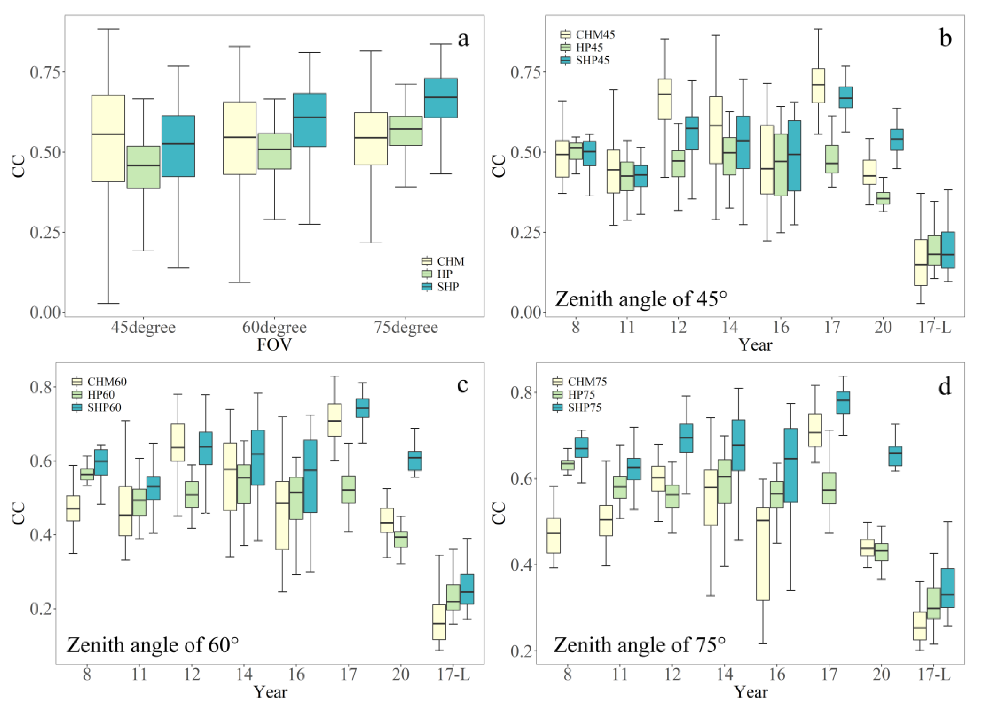
Along with the increase of the FOV, the result range of extracted CC from UAV-LiDAR data by both CHM-based and SHP-based methods becomes narrower (Figure 5a), which indicates that the CHM-based and SHP-based methods with smaller FOV are more sensitive to extract CC. CC extraction from HP, the validation data in this study, had a narrower data range than the CC extracted from UAV-LiDAR (Figure 5a). The extracted CC results by HP classification and the SHP-based method increased according to the increase of the zenith angle range from 45° to 75°, while the extracted results by the CHM-based method are not sensitive to the FOV change (Figure 5a). The performance of CC extraction based on the three methods was different in the poplar plantations with different stand ages (Figure 5b–d). The range of the extracted value of CC by the three methods was relatively consistent in the 45° zenith angle range comparing to that in the 60° and 75° zenith angle ranges (Figure 5b). Comparing to the CC extraction from the HP classification, the CC extraction by the CHM-based method had an underestimation trend along with the increasing FOV (Figure 5c,d).
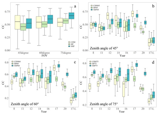
Figure 5.
The extracted CC in the poplar plots using HP and UAV-LiDAR data. (a) The overall range of CC extracted by three methods in different FOVs. (b–d) Boxplots for the HP, CHM-based and SHP-based methods of CC extraction with three FOVs from poplar plantations with different ages. The 17-L represents a leaf-off poplar plantation caused by soil acidification in the 17-year-old plantations.
3.2. Validation of CC Extraction by the CHM-Based Method with the Extraction Results from HP
The relationship between the CC extracted from HP and the CC extracted by the CHM-based model fit the broke-line relationship instead of a simple linear relationship (Figure 6). It indicated that the CC extracted from HP might have a saturation issue in the range of a high CC value, comparing to the CC extract by the CHM-based method with a hemispherical FOV. The validation model had different responses for the CHM-based method with different FOVs (Figure 6). Among all the three validation models (i.e., 45°, 60° and 75° zenith angle ranges; Figure 6), the model with a 45° zenith angle range had the best performance (R2 = 0.751, RMSE = 0.053; Figure 6a) with a segmented point of 0.537. The model with a 60° zenith angle range had a similar result with the zenith angle of 45° (R2 = 0.707, RMSE = 0.053; Figure 6b) with a segmented point of 0.518. However, the validation model with a 75° zenith angle range shows a lower correlation between the CC extracted from the CHM-based and HP method (R2 = 0.490, RMSE = 0.066; Figure 6c), and its segmented point was much lower (0.320) due to the underestimate of CC extracted by the CHM-based method in many locations.

Figure 6.
Validation of CC estimation by the CHM-based method with three zenith angles ((a): 45°, (b): 60°and (c): 75°). The red line is the trend line of a single linear regression. The blue line is the trend line of the broke-line regression. The 1:1 line is displayed as a black oblique dash line. The segmented position is displayed as a black vertical dash line. The spatial resolution of CHM images is 0.5 m, and the range coefficient for the radius is 2.
Different spatial resolutions of CHM images also had an impact on the accuracy of the model (Table 2). Along with the decreasing CHM pixel size, the accuracy of the model gradually declined for all the FOVs. The model accuracy declined faster from the 0.5 m to 2.0 m and from the 2.0 to 5.0 m spatial resolutions in a 45° zenith angle range than in the 60° and 75° zenith angle ranges (Table 2). In other words, the model accuracy was relatively stable in the 60° and 75° zenith angle ranges (Table 2).

Table 2.
Accuracy assessments of CHM-based models of varying spatial resolutions (the range coefficient for the radius is 2).
The different radius of the CHM analysis window (i.e., different range coefficient (k) for radius) also had an influence on the model’s accuracy (Table 3). There was an obvious decline of model accuracy in the 45° zenith angle range, along with the reduction of the radius range (i.e., the range coefficient for radius (k) from 2 to 3). A slight decline of accuracy was observed in the 60° zenith angle range when k changes from 2 to 3. However, the model accuracy had a great improvement for the validation model with the 75° zenith angle range (i.e., R2 increased from 0.490 to 0.589; RMSE decreased from 0.066 to 0.059).

Table 3.
Accuracy assessments of the CHM-based models of varying areas (the resolution of CHM is 0.5 m).
3.3. Validation of CC Extraction by the SHP-Based Method with the Extraction Results from HP
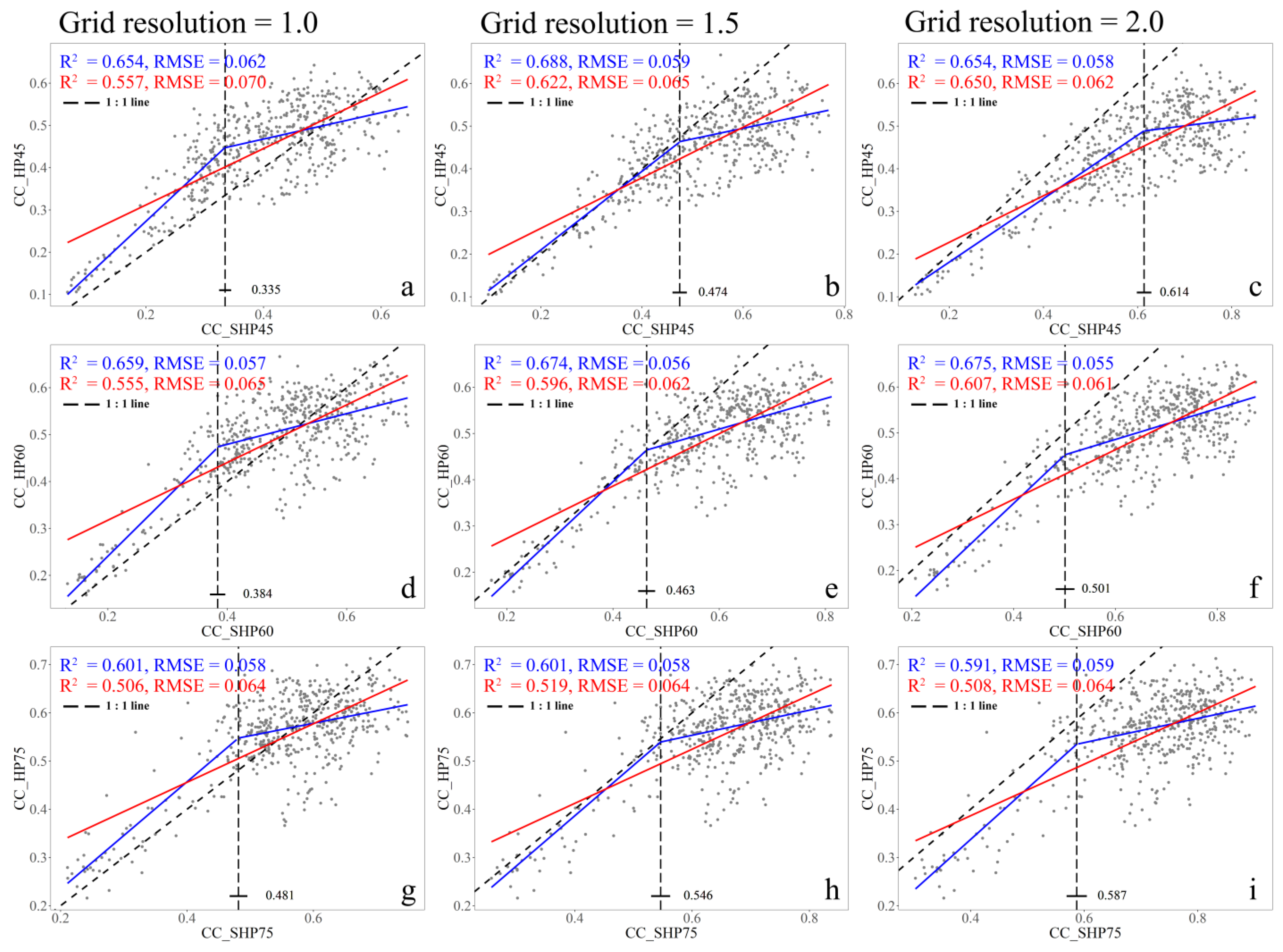
Comparing to the CC extraction from HP, the SHP-based models also had a good performance in the CC extraction from UAV-LiDAR data (Figure 7). The validation models for the relationship between the CC extraction with the SHP-based method and the CC extraction from HP fit the broke-line relationship better than a simple linear relationship (Figure 7), which also indicated that the CC extraction from HP might have a saturation issue in the range of the high CC value, comparing to the extraction results with the SHP-based method in all three FOVs. The grid resolution has slight effects on the model accuracy. The SHP-based method with a 1.5 grid resolution showed the best fit along with the 1:1 line before the segmented point (Figure 7b,e,h). However, comparing with the results from HP, the extraction with the SHP-based model showed an underestimation and overestimation in the range of lower CC values before the segmented point with a grid resolution of 1.0 and 2.0, respectively (Figure 7). With the optimum grid resolution of 1.5, the validation model in a 45° zenith angle range had the best performance (R2 = 0.688; RMSE = 0.065; the segmented point is 0.474; Figure 7b), and the model in a 60° zenith angle range had a similar result (R2 = 0.674; RMSE = 0.062; the segmented point is 0.463; Figure 7e). However, the model in a 75° zenith angle range had a slightly lower performance (R2 = 0.601; RMSE = 0.064; the segmented point is 0.546; Figure 7h).
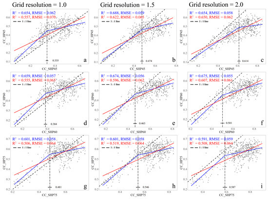
Figure 7.
Validation of the field measured CC and prediction of CC by the SHP-based method with three zenith angles ((a–c): 45°, (d–f): 60°and (g–i): 75°). The red line is the trend line of the single linear regression. The blue line is the trend line of the broke-line regression. The 1:1 line is displayed as a black oblique dash line. The segmented position is displayed as a black vertical dash line. The grid resolutions are 1.0 (a,d,g), 1.5 (b,e,h) and 2.0 (c,f,i).
4. Discussion
4.1. The Advantages and Disadvantages of CC Extraction from UAV-LiDAR Data by CHM-Based and SHP-Based Methods with a Hemispherical FOV
The extracted CC based on the CHM and SHP data had a good relationship and similar regression trends with the CC extraction from HP classification. Another similarity between the two methods using UAV-LiDAR data was that they both have the best performance at the zenith angle of 45° compared to that of 60° and 75° (Figure 5, Figure 6 and Figure 7). The accuracy of the two models decreases with the increase of FOV, which was more obvious in the CHM-based model (Figure 6 and Figure 7). One possible reason was that the CHM-based method does not correspond well to a ground-based hemispherical FOV for a large zenith angle [11,37]. A previous study also showed that the CHM-based method might have a better description for the spatial averages of CC [44]. This could be confirmed with the CC results of the CHM-based model with the zenith angle range increase (Figure 5a), which might be the main reason why the accuracy of the CHM-based model continues to decrease with the increase of the FOV. Another interesting phenomenon was that the SHP-based model’s result was usually consistent with the 1:1 line before the segmented point, while the CHM result showed an underestimation (Figure 6 and Figure 7). In addition to the reasons above, another reason was that the CHM-based method would underestimate CC for leaf-off deciduous trees (i.e., “17-L” in Figure 5) because the pulses of UAV-LiDAR were more likely to pass between the branches [37]. Overall, the SHP-based model describes the change of the ground hemisphere FOV better than the CHM-based method based on UAV-LiDAR data.
Although the SHP-based model was relatively stable, its accuracy slightly decreased with the increase of the FOV (Figure 7), which might be related to the coverage range of the point cloud and the geographic conditions of poplar plantations [41]. We used the algorithm of SHP to meet the range of the zenith angle as much as possible, but the range of the laser pulse is limited and it is hard to detecting the objects far from the shooting location. Moreover, the point cloud data had been normalized to eliminate the impact of the terrain, which cannot be achieved in the HP classification. Other factors, including understory vegetation, the unevenness of foliage lighting, the noise effects of UAV-LiDAR and other differences between HP and LiDAR data might be magnified in the range of a high zenith angle [64].
The spatial resolution had some impact on the accuracy of the CHM-based model, but the CC extraction results were still robust even when we increase the spatial resolution to 5 m (Table 2). The accuracy of the CHM-based model had a pronounced decline with the decrease of spatial resolution at a low zenith angle range (i.e., 45°). The gap fraction of the canopy was more sensitive to the CC extraction with the range of the low zenith angle, and the small canopy gap might not be the primary factor in CC extraction with a lager zenith angle range [37]. However, the SHP-based method showed a better robustness with the grid resolution change (Figure 7). On the one hand, the grid resolution interval of the SHP-based method was not very large. On the other hand, the SHP-based method is more accurate for the description of the canopy gap in a FOV range [48].
Our radius model of the CHM-based method had different CC extraction results in different zenith angle ranges, and the different distance coefficient () provided a probable reference for it. The fixed radius range was not suitable for our study because of the distinguishing difference of tree height between the plots. A diverse FOV was also a big challenge to the accurate radius model. To improve the accuracy of the CHM-based model, it is necessary to find a better radius model or improve the CHM-based algorithm in subsequent research. However, the range of area in the SHP-based method was simple, and the only need was to determine the theoretical maximum horizontal radius at the maximum zenith angle to obtain the same result as the ground FOV [13,44,45], which was verified by the visualization results of the SHP algorithm (Figure 4). The point cloud density’s unevenness in different plots might have an effect on the results [57], but this impact was eliminated by thinning the point clouds of all sample plots.
4.2. The Accuracy of the Validation Data (CC Extraction from HP)
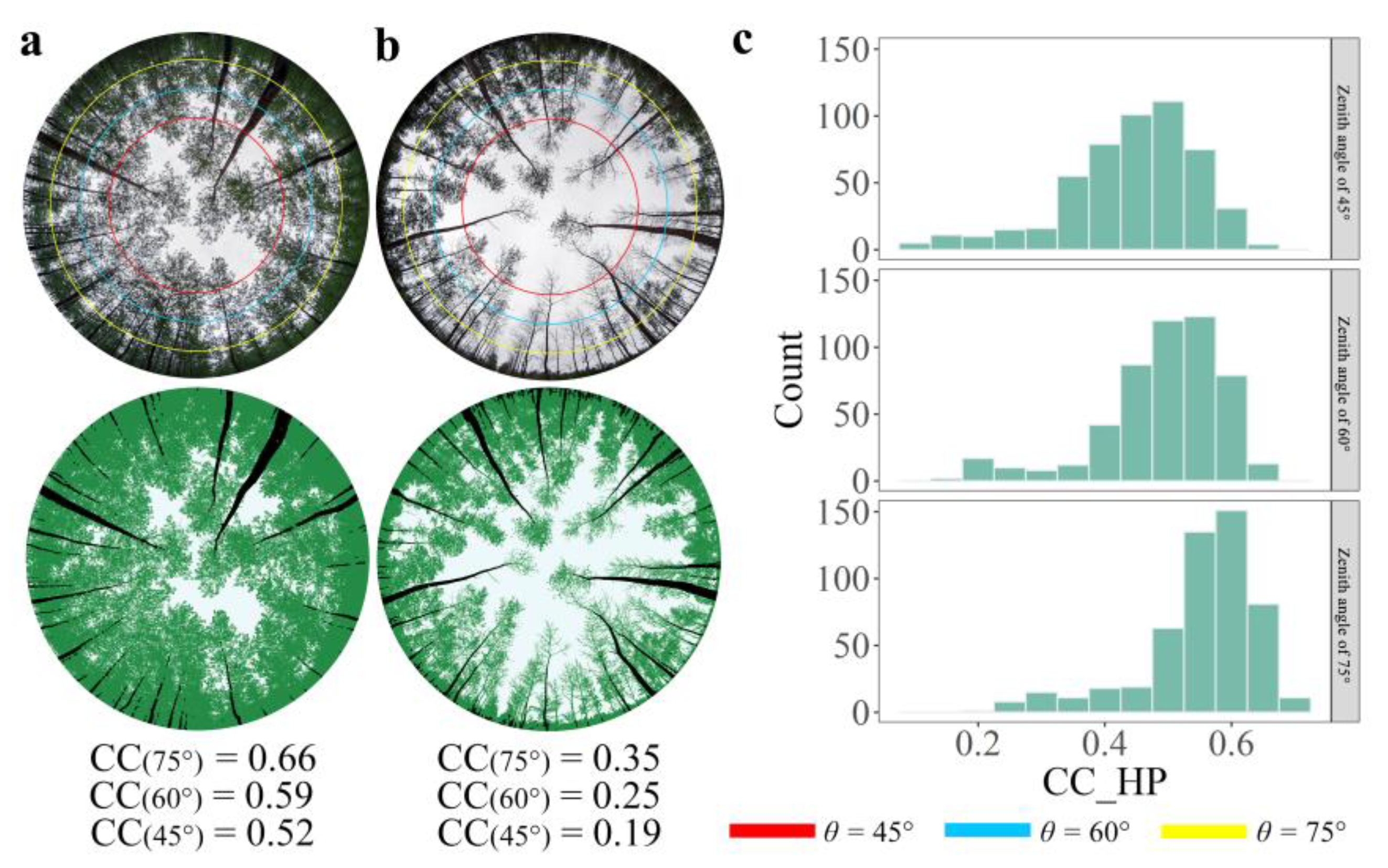
The validation data were extracted from HP in three zenith angle ranges (Figure 8). The distribution of CC in different FOVs was different from the histogram of the results (Figure 8c), and this distribution pattern appeared both in high and low CC conditions (Figure 8a,b). Overall, the extracted CC from HP is larger when the zenith angle is larger, which is consistent with Fiala et al.’s results [65]. The accuracy of the HP method was robust in three zenith angle ranges (Table 4). The overall accuracy of all plots was highest in the zenith angle of 45° (F = 0.967), followed by the zenith angle of 75° (F = 0.942) and the zenith angle of 60° (F = 0.938).
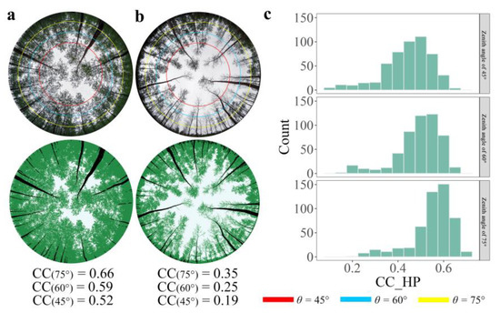
Figure 8.
Results of CC extraction from field sites. (a) Example of a HP method result in a high CC situation. (b) Example of a HP method result in a low CC situation. (c) The CC for hemispherical photographs covers the range from 0.1 to 0.8 with three zenith angles. The green, black and white pixels in (a,b) represent canopy pixel, trunk pixel and sky pixel, respectively. is the zenith angle in HP.

Table 4.
The accuracy assessments for the HP method with three zenith angles.
In the study, we improved the accuracy of CC extraction in HP by removing the main trunk of poplar trees because the tree trunks account for a certain percentage (Figure 8a,b). In addition, the UAV-LiDAR system could describe the tree crown well, but had difficulty in describing the trunk [66], so it is necessary to eliminate the trunk’s influence in HP. HP is essentially a two-dimensional passive sensor in a hemisphere FOV [14], which is different from the UAV-LiDAR point cloud data. Thus, there is a certain underestimate after removing the trunks in HP. Moreover, HP data and UAV-LiDAR data are sensitive to different factors (i.e., sensor differences and sensitivity to the environment) in the CC extraction. In addition to the difference in sensor parameters, the accuracy of the CC results from HP is more sensitive to environmental factors, such as radiometric condition, terrain, wind, unevenness of foliage lighting and the choice of subjective threshold, which would increase this uncertainty [14,41].
4.3. Stand Age Effects on the Model Accuracy for CC Extraction
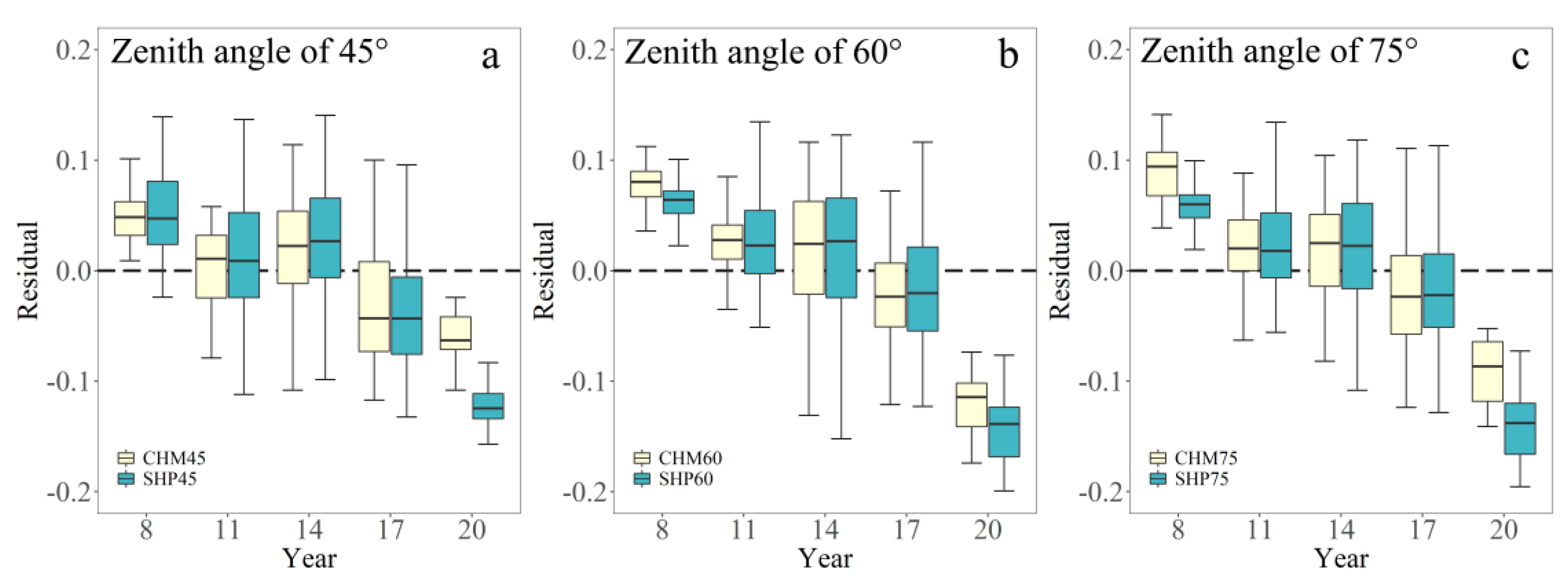
The residual boxplot distribution results were similar in the young poplar plantations (i.e., 8, 11 and 14 years old) in the 45° zenith angle range. A significant overestimation of the CC extraction from UAV-LiDAR data was observed in the old plantations (i.e., 17 and 20 years old; Figure 9a). However, by the CHM-based models, the results appeared an underestimation in the young plantations and an overestimation in the old plantations with the 60° and 75° zenith angle ranges (Figure 9b,c). This phenomenon also appeared in the results of the SHP-based method, but the underestimation was slighter in the 8-year-old plantations and more obvious in the 20-year-old plantations (Figure 9b,c). However, along with the increase of the zenith angle range, there was an obvious increase of the CC value extracted by the HP and SHP-based methods, while there was no significant change by the CHM-based method (Table 5). The characteristics of the CHM-based method, which had a better description for the spatial averages of CC, cause this phenomenon (see the description in Section 4.1 for a detailed discussion).
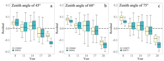
Figure 9.
Residual boxplots for the CHM-based and SHP-based models in plantations with different ages with three zenith angles ((a): 45°, (b): 60°and (c): 75°). The resolution is 0.5 m, and the range coefficient for the radius is 2 with the CHM-based models. The grid resolution is 1.5 with the SHP-based models.

Table 5.
The growth rate of HP, SHP-based and the CHM-based method for each 15° zenith angle increase in plantations with different ages. The mean is the average growth rate of 45–60° and 60–75°.
The distinguished differences in the extraction of CC in young poplar plantations and old poplar plantations had a great impact on the accuracy of the model. The variety of tree heights in different ages plots is the main reason for the difference in CC extractions, and different structures in the poplar age plots would affect the extraction accuracy as well [13,67]. The longer distance between the camera lens and the tree canopy lead to a low resolution of the canopy, which brings errors in the CC extraction of HP [61,68]. Another reason is the difference of light conditions between plots, because we found there was a slight exposure in HP of these old poplar plantations, especially at the larger zenith angle. Thus, this might be due to the underestimation of CC from HP instead of the overestimation of CC from the UAV-LiDAR point cloud data in old poplar plantations, because the photographs are more sensitive to changes of the environment [41,64]. The age effects caused by the limitation of the camera sensor led to a saturation tendency in the model. However, the regression relationship of the model under the same age plot is theoretically linear. One way of eliminating age effects is to consider regression models for each age plot, but it might not be effective in plantations with uniform planting density, because the narrow range of CC often leads to an insignificant regression relationship in the model [69]. Another way is to find a balance coefficient to normalize all plots, but it is also a challenge due to the difficulty of quantifying complex environmental conditions. Further research is needed to assess the age effects and how to eliminate them.
Overall, the UAV-LiDAR system can obtain reliable forest CC information over extensive areas. This is also a good way to store the 3D information of the forest canopy, in which there is an agreement of the extracted CC results with the hemispherical photos taken in the same location. The automatic CC extraction from UAV-LiDAR data would benefit the description of understory light conditions as well, which is consistent with the finding, in the previous study, that CC extraction is promising for assessing regional solar radiation metrics [70]. Moreover, CC often have a strong relationship with various forest parameters. Thus, our results and methods of CC extraction can become good references for further studies on the extraction of other forest parameters in plantation forests.
5. Conclusions
Both CHM-based and SHP-based methods show a good performance when extracting CC from UAV-LiDAR data in poplar plantations with a uniform planting density. The CHM-based method had the highest accuracy in a 45° zenith angle range ( = 0.751, = 0.053), and the accuracy showed a decline when choosing a zenith angle of 60° and 75° ( = 0.707, 0.490; = 0.053, 0.066). The higher resolution of pixel size enhances the performance of CC extraction by the CHM-based model, and a suitable radius of the CHM analysis window is another factor which can mitigate the bias in the model. The accuracy of the SHP-based method was stable in three zenith angle ranges (: 0.688, 0.674, 0.601 and = 0.059, 0.056, 0.058 for 45°, 60° and 75° zenith angle ranges), and it showed a better consistency with the 1:1 line before the segmented point. Comparing to the HP results, the CC extracted from UAV-LiDAR data showed an overestimation in old poplar plantation plots due to the difference between camera and LiDAR sensors. Compared to the HP results, the SHP-based method was more sensitive to the FOV changes than the CHM-based method. Based on our research, the SHP-based model had a better performance in CC extraction than the CHM-based method in different FOVs. Our research proved that the UAV-LiDAR data are useful for CC estimation in forest plantation, which provided a reasonable reference for monitoring regional understory lighting conditions in the future.
Supplementary Materials
The following are available online at https://www.mdpi.com/article/10.3390/rs13193837/s1. Python scripts, ArcToolbox.
Author Contributions
Y.P. contributed by developing the methodology, writing the python script, analyzing the data and writing the manuscript. D.X. contributed by coming up with the initial ideas, guiding the research directions and revising the manuscript. H.W. and D.A. contributed to the field work design, field data collection and data analysis. X.X. contributed by providing information of the study area and interpreting the research results. All authors have read and agreed to the published version of the manuscript.
Funding
This study was funded by the National Natural Science Foundation of China (41901361), the Six Talent Peaks Project in Jiangsu Province (TD-XYDXX-006), the Natural Science Foundation of Jiangsu Province (BK20180769) and the Major Basic Research Project of the Natural Science Foundation of the Jiangsu Higher Education Institutions (18KJB180009).
Acknowledgments
The authors would like to acknowledge the field crew for collecting the field data.
Conflicts of Interest
The authors declare no conflict of interest.
References
- Hartley, M.J. Rationale and methods for conserving biodiversity in plantation forests. For. Ecol. Manag. 2002, 155, 81–95. [Google Scholar] [CrossRef]
- Pawson, S.M.; Brin, A.; Brockerhoff, E.G.; Lamb, D.; Payn, T.W.; Paquette, A.; Parrotta, J.A. Plantation forests, climate change and biodiversity. Biodivers. Conserv. 2013, 22, 1203–1227. [Google Scholar] [CrossRef]
- Wang, G.B.; Deng, F.F.; Xu, W.H.; Chen, H.Y.H.; Ruan, H.H.; Goss, M. Poplar plantations in coastal China: Towards the identification of the best rotation age for optimal soil carbon sequestration. Soil Use Manag. 2016, 32, 303–310. [Google Scholar] [CrossRef]
- Meroni, M.; Colombo, R.; Panigada, C. Inversion of a radiative transfer model with hyperspectral observations for LAI mapping in poplar plantations. Remote Sens. Environ. 2004, 92, 195–206. [Google Scholar] [CrossRef]
- Canham, C.D.; Finzi, A.C.; Pacala, S.W.; Burbank, D.H. Causes and consequences of resource heterogeneity in forests: Interspecific variation in light transmission by canopy trees. Can. J. For. Res. 1994, 24, 337–349. [Google Scholar] [CrossRef]
- Popescu, S.C.; Wynne, R.H. Seeing the trees in the forest: Using lidar and multispectral data fusion with local filtering and variable window size for estimating tree height. Photogramm. Eng. Remote Sens. 2004, 70, 589–604. [Google Scholar] [CrossRef] [Green Version]
- Lee, A.C.; Lucas, R.M. A LiDAR-derived canopy density model for tree stem and crown mapping in Australian forests. Remote Sens. Environ. 2007, 111, 493–518. [Google Scholar] [CrossRef]
- Lieffers, V.J.; Messier, C.; Stadt, K.J.; Gendron, F.; Comeau, P.G. Predicting and managing light in the understory of boreal forests. Can. J. For. Res. 1999, 29, 796–811. [Google Scholar] [CrossRef]
- Korhonen, L.; Korhonen, K.T.; Rautiainen, M.; Stenberg, P. Estimation of forest canopy cover: A comparison of field measurement techniques. Silva. Fenn. 2006, 40, 577–588. [Google Scholar] [CrossRef] [Green Version]
- Jennings, S.B.; Brown, N.D.; Sheil, D. Assessing forest canopies and understorey illumination: Canopy closure, canopy cover and other measures. Forestry 1999, 72, 59–74. [Google Scholar] [CrossRef]
- Korhonen, L.; Korpela, I.; Heiskanen, J.; Maltamo, M. Airborne discrete-return LIDAR data in the estimation of vertical canopy cover, angular canopy closure and leaf area index. Remote Sens. Environ. 2011, 115, 1065–1080. [Google Scholar] [CrossRef]
- Musselman, K.N.; Molotch, N.P.; Margulis, S.A.; Kirchner, P.B.; Bales, R.C. Influence of canopy structure and direct beam solar irradiance on snowmelt rates in a mixed conifer forest. Agric. For. Meteorol. 2012, 161, 46–56. [Google Scholar] [CrossRef]
- Alexander, C.; Moeslund, J.E.; Bocher, P.K.; Arge, L.; Svenning, J.-C. Airborne laser scanner (LiDAR) proxies for understory light conditions. Remote Sens. Environ. 2013, 134, 152–161. [Google Scholar] [CrossRef]
- Zhu, X.; Liu, J.; Skidmore, A.K.; Premier, J.; Heurich, M. A voxel matching method for effective leaf area index estimation in temperate deciduous forests from leaf-on and leaf-off airborne LiDAR data. Remote Sens. Environ. 2020, 240, 111696. [Google Scholar] [CrossRef]
- Wei, S.; Yin, T.; Dissegna, M.A.; Whittle, A.J.; Ow, G.L.F.; Yusof, M.L.M.; Lauret, N.; Gastellu-Etchegorry, J.-P. An assessment study of three indirect methods for estimating leaf area density and leaf area index of individual trees. Agric. For. Meteorol. 2020, 292, 108101. [Google Scholar] [CrossRef]
- Welles, J.M. Some indirect methods of estimating canopy structure. Remote Sens. Rev. 1990, 5, 31–43. [Google Scholar] [CrossRef]
- Jonckheere, I.; Nackaerts, K.; Muys, B.; Coppin, P. Assessment of automatic gap fraction estimation of forests from digital hemispherical photography. Agric. For. Meteorol. 2004, 132, 96–114. [Google Scholar] [CrossRef]
- Jonckheere, I.; Fleck, S.; Nackaerts, K.; Muys, B.; Coppin, P.; Weiss, M.; Baret, F. Review of methods for in situ leaf area index determination—Part I. Theories, sensors and hemispherical photography. Agric. For. Meteorol. 2004, 121, 19–35. [Google Scholar] [CrossRef]
- Danson, F.M.; Hetherington, D.; Morsdorf, F.; Koetz, B.; Allgoewer, B. Forest canopy gap fraction from terrestrial laser scanning. IEEE Geosci. Remote Sens. Lett. 2007, 4, 157–160. [Google Scholar] [CrossRef] [Green Version]
- Thimonier, A.; Sedivy, I.; Schleppi, P. Estimating leaf area index in different types of mature forest stands in Switzerland: A comparison of methods. Eur. J. For. Res. 2010, 129, 543–562. [Google Scholar] [CrossRef]
- Smith, A.M.; Ramsay, P.M. A comparison of ground-based methods for estimating canopy closure for use in phenology research. Agric. For. Meteorol. 2018, 252, 18–26. [Google Scholar] [CrossRef]
- Tao, S.; Wu, F.; Guo, Q.; Wang, Y.; Li, W.; Xue, B.; Hu, X.; Li, P.; Tian, D.; Li, C.; et al. Segmenting tree crowns from terrestrial and mobile LiDAR data by exploring ecological theories. ISPRS-J. Photogramm. Remote Sens. 2015, 110, 66–76. [Google Scholar] [CrossRef] [Green Version]
- Luo, L.; Zhai, Q.; Su, Y.; Ma, Q.; Kelly, M.; Guo, Q. Simple method for direct crown base height estimation of individual conifer trees using airborne LiDAR data. Opt. Express 2018, 26, A562–A578. [Google Scholar] [CrossRef]
- Zhou, H.; Chen, Y.; Feng, Z.; Li, F.; Hyyppa, J.; Hakala, T.; Karjalainen, M.; Jiang, C.; Pei, L. The Comparison of Canopy Height Profiles Extracted from Ku-band Profile Radar Waveforms and LiDAR Data. Remote Sens. 2018, 10, 701. [Google Scholar] [CrossRef] [Green Version]
- Rostami, M.; Kolouri, S.; Eaton, E.; Kim, K. SAR Image Classification Using Few-Shot Cross-Domain Transfer Learning. In Proceedings of the 2019 IEEE/CVF Conference on Computer Vision and Pattern Recognition Workshops (CVPRW), Long Beach, CA, USA, 16–17 June 2019; pp. 907–915. [Google Scholar]
- Pardini, M.; Armston, J.; Qi, W.; Lee, S.K.; Tello, M.; Cazcarra Bes, V.; Choi, C.; Papathanassiou, K.P.; Dubayah, R.O.; Fatoyinbo, L.E. Early Lessons on Combining Lidar and Multi-baseline SAR Measurements for Forest Structure Characterization. Surv. Geophys. 2019, 40, 803–837. [Google Scholar] [CrossRef]
- Cao, C.; Bao, Y.; Xu, M.; Chen, W.; Zhang, H.; He, Q.; Li, Z.; Guo, H.; Li, J.; Li, X.; et al. Retrieval of forest canopy attributes based on a geometric-optical model using airborne LiDAR and optical remote-sensing data. Int. J. Remote Sens. 2012, 33, 692–709. [Google Scholar] [CrossRef]
- Ma, Q.; Su, Y.; Guo, Q. Comparison of Canopy Cover Estimations From Airborne LiDAR, Aerial Imagery, and Satellite Imagery. IEEE J. Sel. Top. Appl. Earth Observ. Remote Sens. 2017, 10, 4225–4236. [Google Scholar] [CrossRef]
- Lefsky, M.A.; Cohen, W.B.; Acker, S.A.; Parker, G.G.; Spies, T.A.; Harding, D. Lidar remote sensing of the canopy structure and biophysical properties of Douglas-fir western hemlock forests. Remote Sens. Environ. 1999, 70, 339–361. [Google Scholar] [CrossRef]
- Zhang, Y.; Shao, Z. Assessing of Urban Vegetation Biomass in Combination with LiDAR and High-resolution Remote Sensing Images. Int. J. Remote Sens. 2020, 42, 964–985. [Google Scholar] [CrossRef]
- Shen, X.; Cao, L. Tree-Species Classification in Subtropical Forests Using Airborne Hyperspectral and LiDAR Data. Remote Sens. 2017, 9, 1180. [Google Scholar] [CrossRef] [Green Version]
- Parent, J.R.; Volin, J.C. Assessing species-level biases in tree heights estimated from terrain-optimized leaf-off airborne laser scanner (ALS) data. Int. J. Remote Sens. 2015, 36, 2697–2712. [Google Scholar] [CrossRef]
- Hopkinson, C. The influence of flying altitude, beam divergence, and pulse repetition frequency on laser pulse return intensity and canopy frequency distribution. Can. J. Remote Sens. 2007, 33, 312–324. [Google Scholar] [CrossRef]
- McLane, A.J.; McDermid, G.J.; Wulder, M.A. Processing discrete-return profiling lidar data to estimate canopy closure for large-area forest mapping and management. Can. J. Remote Sens. 2009, 35, 217–229. [Google Scholar] [CrossRef]
- Hopkinson, C.; Chasmer, L. Testing LiDAR models of fractional cover across multiple forest ecozones. Remote Sens. Environ. 2009, 113, 275–288. [Google Scholar] [CrossRef]
- Torresani, M.; Rocchini, D.; Sonnenschein, R.; Zebisch, M.; Hauffe, H.C.; Heym, M.; Pretzsch, H.; Tonon, G. Height variation hypothesis: A new approach for estimating forest species diversity with CHM LiDAR data. Ecol. Indic. 2020, 117, 106520. [Google Scholar] [CrossRef]
- Parent, J.R.; Volin, J.C. Assessing the potential for leaf-off LiDAR data to model canopy closure in temperate deciduous forests. ISPRS-J. Photogramm. Remote Sens. 2014, 95, 134–145. [Google Scholar] [CrossRef]
- Riano, D.; Valladares, F.; Condes, S.; Chuvieco, E. Estimation of leaf area index and covered ground from airborne laser scanner (Lidar) in two contrasting forests. Agric. For. Meteorol. 2004, 124, 269–275. [Google Scholar] [CrossRef]
- Bunce, A.; Volin, J.C.; Miller, D.R.; Parent, J.; Rudnicki, M. Determinants of tree sway frequency in temperate deciduous forests of the Northeast United States. Agric. For. Meteorol. 2019, 266, 87–96. [Google Scholar] [CrossRef] [Green Version]
- Seidel, D.; Fleck, S.; Leuschner, C. Analyzing forest canopies with ground-based laser scanning: A comparison with hemispherical photography. Agric. For. Meteorol. 2012, 154, 1–8. [Google Scholar] [CrossRef]
- Hancock, S.; Essery, R.; Reid, T.; Carle, J.; Baxter, R.; Rutter, N.; Huntley, B. Characterising forest gap fraction with terrestrial lidar and photography: An examination of relative limitations. Agric. For. Meteorol. 2014, 189, 105–114. [Google Scholar] [CrossRef] [Green Version]
- Perez, R.P.A.; Costes, E.; Theveny, F.; Griffon, S.; Caliman, J.-P.; Dauzat, J. 3D plant model assessed by terrestrial LiDAR and hemispherical photographs: A useful tool for comparing light interception among oil palm progenies. Agric. For. Meteorol. 2018, 249, 250–263. [Google Scholar] [CrossRef]
- Varhola, A.; Frazer, G.W.; Teti, P.; Coops, N.C. Estimation of forest structure metrics relevant to hydrologic modelling using coordinate transformation of airborne laser scanning data. Hydrol. Earth Syst. Sci. 2012, 16, 3749–3766. [Google Scholar] [CrossRef] [Green Version]
- Moeser, D.; Roubinek, J.; Schleppi, P.; Morsdorf, F.; Jonas, T. Canopy closure, LAI and radiation transfer from airborne LiDAR synthetic images. Agric. For. Meteorol. 2014, 197, 158–168. [Google Scholar] [CrossRef]
- Zellweger, F.; Baltensweiler, A.; Schleppi, P.; Huber, M.; Kuchler, M.; Ginzler, C.; Jonas, T. Estimating below-canopy light regimes using airborne laser scanning: An application to plant community analysis. Ecol. Evol. 2019, 9, 9149–9159. [Google Scholar] [CrossRef] [PubMed] [Green Version]
- Chianucci, F.; Disperati, L.; Guzzi, D.; Bianchini, D.; Nardino, V.; Lastri, C.; Rindinella, A.; Corona, P. Estimation of canopy attributes in beech forests using true colour digital images from a small fixed-wing UAV. Int. J. Appl. Earth Obs. Geoinf. 2016, 47, 60–68. [Google Scholar] [CrossRef] [Green Version]
- Adão, T.; Hruška, J.; Pádua, L.; Bessa, J.; Peres, E.; Morais, R.; Sousa, J. Hyperspectral Imaging: A Review on UAV-Based Sensors, Data Processing and Applications for Agriculture and Forestry. Remote Sens. 2017, 9, 1110. [Google Scholar] [CrossRef] [Green Version]
- Bruellhardt, M.; Rotach, P.; Schleppi, P.; Bugmann, H. Vertical light transmission profiles in structured mixed deciduous forest canopies assessed by UAV-based hemispherical photography and photogrammetric vegetation height models. Agric. For. Meteorol. 2020, 281, 107843. [Google Scholar] [CrossRef]
- Beland, M.; Parker, G.; Sparrow, B.; Harding, D.; Chasmer, L.; Phinn, S.; Antonarakis, A.; Strahler, A. On promoting the use of lidar systems in forest ecosystem research. For. Ecol. Manag. 2019, 450, 117484. [Google Scholar] [CrossRef]
- Feng, Q.; Yang, J.; Liu, Y.; Ou, C.; Zhu, D.; Niu, B.; Liu, J.; Li, B. Multi-Temporal Unmanned Aerial Vehicle Remote Sensing for Vegetable Mapping Using an Attention-Based Recurrent Convolutional Neural Network. Remote Sens. 2020, 12, 1668. [Google Scholar] [CrossRef]
- Guimarães, N.; Pádua, L.; Marques, P.; Silva, N.; Peres, E.; Sousa, J.J. Forestry Remote Sensing from Unmanned Aerial Vehicles: A Review Focusing on the Data, Processing and Potentialities. Remote Sens. 2020, 12, 1046. [Google Scholar] [CrossRef] [Green Version]
- Cao, L.; Liu, H.; Fu, X.; Zhang, Z.; Shen, X.; Ruan, H. Comparison of UAV LiDAR and Digital Aerial Photogrammetry Point Clouds for Estimating Forest Structural Attributes in Subtropical Planted Forests. Forests 2019, 10, 145. [Google Scholar] [CrossRef] [Green Version]
- Wallace, L.; Lucieer, A.; Watson, C.; Turner, D. Development of a UAV-LiDAR System with Application to Forest Inventory. Remote Sens. 2012, 4, 1519–1543. [Google Scholar] [CrossRef] [Green Version]
- Wu, X.; Shen, X.; Cao, L.; Wang, G.; Cao, F. Assessment of Individual Tree Detection and Canopy Cover Estimation using Unmanned Aerial Vehicle based Light Detection and Ranging (UAV-LiDAR) Data in Planted Forests. Remote Sens. 2019, 11, 908. [Google Scholar] [CrossRef] [Green Version]
- Yan, W.; Guan, H.; Cao, L.; Yu, Y.; Li, C.; Lu, J. A Self-Adaptive Mean Shift Tree-Segmentation Method Using UAV LiDAR Data. Remote Sens. 2020, 12, 515. [Google Scholar] [CrossRef] [Green Version]
- Brede, B.; Lau, A.; Bartholomeus, H.M.; Kooistra, L. Comparing RIEGL RiCOPTER UAV LiDAR Derived Canopy Height and DBH with Terrestrial LiDAR. Sensors 2017, 17, 2371. [Google Scholar] [CrossRef]
- Liu, K.; Shen, X.; Cao, L.; Wang, G.; Cao, F. Estimating forest structural attributes using UAV-LiDAR data in Ginkgo plantations. ISPRS-J. Photogramm. Remote Sens. 2018, 146, 465–482. [Google Scholar] [CrossRef]
- Li, Y.; Chen, Y.; Xu, C.; Xu, H.; Zou, X.; Chen, H.Y.H.; Ruan, H. The abundance and community structure of soil arthropods in reclaimed coastal saline soil of managed poplar plantations. Geoderma 2018, 327, 130–137. [Google Scholar] [CrossRef]
- Glira, P.; Pfeifer, N.; Briese, C.; Ressl, C. A Correspondence Framework for ALS Strip Adjustments based on Variants of the ICP Algorithm. Photogramm. Fernerkund. Geoinf. 2015, 275–289. [Google Scholar] [CrossRef]
- Zhao, X.; Guo, Q.; Su, Y.; Xue, B. Improved progressive TIN densification filtering algorithm for airborne LiDAR data in forested areas. ISPRS-J. Photogramm. Remote Sens. 2016, 117, 79–91. [Google Scholar] [CrossRef] [Green Version]
- Woodgate, W.; Jones, S.D.; Suarez, L.; Hill, M.J.; Armston, J.D.; Wilkes, P.; Soto-Berelov, M.; Haywood, A.; Mellor, A. Understanding the variability in ground-based methods for retrieving canopy openness, gap fraction, and leaf area index in diverse forest systems. Agric. For. Meteorol. 2015, 205, 83–95. [Google Scholar] [CrossRef]
- Solberg, S.; Brunner, A.; Hanssen, K.H.; Lange, H.; Næsset, E.; Rautiainen, M.; Stenberg, P. Mapping LAI in a Norway spruce forest using airborne laser scanning. Remote Sens. Environ. 2009, 113, 2317–2327. [Google Scholar] [CrossRef]
- Leblanc, S.G.; Chen, J.M.; Fernandes, R.; Deering, D.W.; Conley, A. Methodology comparison for canopy structure parameters extraction from digital hemispherical photography in boreal forests. Agric. For. Meteorol. 2005, 129, 187–207. [Google Scholar] [CrossRef] [Green Version]
- Zhu, X.; Skidmore, A.K.; Wang, T.; Liu, J.; Darvishzadeh, R.; Shi, Y.; Premier, J.; Heurich, M. Improving leaf area index (LAI) estimation by correcting for clumping and woody effects using terrestrial laser scanning. Agric. For. Meteorol. 2018, 263, 276–286. [Google Scholar] [CrossRef]
- Fiala, A.C.S.; Garman, S.L.; Gray, A.N. Comparison of five canopy cover estimation techniques in the western Oregon Cascades. For. Ecol. Manag. 2006, 232, 188–197. [Google Scholar] [CrossRef]
- Lu, J.; Wang, H.; Qin, S.; Cao, L.; Pu, R.; Li, G.; Sun, J. Estimation of aboveground biomass of Robinia pseudoacacia forest in the Yellow River Delta based on UAV and Backpack LiDAR point clouds. Int. J. Appl. Earth Obs. Geoinf. 2020, 86. [Google Scholar] [CrossRef]
- Lovell, J.L.; Jupp, D.L.B.; Culvenor, D.S.; Coops, N.C. Using airborne and ground-based ranging lidar to measure canopy structure in Australian forests. Can. J. Remote Sens. 2003, 29, 607–622. [Google Scholar] [CrossRef]
- Macfarlane, C. Classification method of mixed pixels does not affect canopy metrics from digital images of forest overstorey. Agric. For. Meteorol. 2011, 151, 833–840. [Google Scholar] [CrossRef]
- Wasser, L.; Day, R.; Chasmer, L.; Taylor, A. Influence of Vegetation Structure on Lidar-derived Canopy Height and Fractional Cover in Forested Riparian Buffers During Leaf-Off and Leaf-On Conditions. PLoS ONE 2013, 8, e54776. [Google Scholar] [CrossRef] [Green Version]
- Moeser, D.; Morsdorf, F.; Jonas, T. Novel forest structure metrics from airborne LiDAR data for improved snow interception estimation. Agric. For. Meteorol. 2015, 208, 40–49. [Google Scholar] [CrossRef]
Publisher’s Note: MDPI stays neutral with regard to jurisdictional claims in published maps and institutional affiliations. |
© 2021 by the authors. Licensee MDPI, Basel, Switzerland. This article is an open access article distributed under the terms and conditions of the Creative Commons Attribution (CC BY) license (https://creativecommons.org/licenses/by/4.0/).

