Abstract
We apply the Support Vector Regression (SVR) machine learning model to estimate surface roughness on a large alluvial fan of the Kosi River in the Himalayan Foreland from satellite images. To train the model, we used input features such as radar backscatter values in Vertical–Vertical (VV) and Vertical–Horizontal (VH) polarisation, incidence angle from Sentinel-1, Normalised Difference Vegetation Index (NDVI) from Sentinel-2, and surface elevation from Shuttle Radar Topographic Mission (SRTM). We generated additional features (VH/VV and VH–VV) through a linear data fusion of the existing features. For the training and validation of our model, we conducted a field campaign during 11–20 December 2019. We measured surface roughness at 78 different locations over the entire fan surface using an in-house-developed mechanical pin-profiler. We used the regression tree ensemble approach to assess the relative importance of individual input feature to predict the surface soil roughness from SVR model. We eliminated the irrelevant input features using an iterative backward elimination approach. We then performed feature sensitivity to evaluate the riskiness of the selected features. Finally, we applied the dimension reduction and scaling to minimise the data redundancy and bring them to a similar level. Based on these, we proposed five SVR methods (PCA-NS-SVR, PCA-CM-SVR, PCA-ZM-SVR, PCA-MM-SVR, and PCA-S-SVR). We trained and evaluated the performance of all variants of SVR with a 60:40 ratio using the input features and the in-situ surface roughness. We compared the performance of SVR models with six different benchmark machine learning models (i.e., Gaussian Process Regression (GPR), Generalised Regression Neural Network (GRNN), Binary Decision Tree (BDT), Bragging Ensemble Learning, Boosting Ensemble Learning, and Automated Machine Learning (AutoML)). We observed that the PCA-MM-SVR perform better with a coefficient of correlation (R = 0.74), Root Mean Square Error (RMSE = 0.16 cm), and Mean Square Error (MSE = 0.025 ). To ensure a fair selection of the machine learning model, we evaluated the Akaike’s Information Criterion (AIC), corrected AIC (AICc), and Bayesian Information Criterion (BIC). We observed that SVR exhibits the lowest values of AIC, corrected AIC, and BIC of all the other methods; this indicates the best goodness-of-fit. Eventually, we also compared the result of PCA-MM-SVR with the surface roughness estimated from different empirical and semi-empirical radar backscatter models. The accuracy of the PCA-MM-SVR model is better than the backscatter models. This study provides a robust approach to measure surface roughness at high spatial and temporal resolutions solely from the satellite data.
1. Introduction
Surface soil roughness is an important parameter in many environmental applications, such as: agronomy, geomorphology, hydrology, meteorology, and climate change modeling [1,2]. By definition, surface roughness is a non-zero Gaussian random process that is parameterised by the Root Mean Square (RMS) height (s), and correlation length (l). The root mean square height describes the vertical roughness, whereas the correlation length is used to describe roughness at a horizontal scale. Usually, surface roughness measured in the horizontal scale is subject to large variability and uncertainty as compared to the vertical scale [3]. This is probably one reason that RMS height is used in the inversion of various backscattering models [4]. The surface roughness (RMS height) is considered a highly sensitive parameter in modeling soil moisture from the Synthetic Aperture Radar (SAR) images [5]. It is important to have an accurate measurement of surface roughness in order to model the soil moisture from SAR images [6].
Surface soil roughness can be categorised into four different scales, such as the microrelief, random, oriented roughness, and higher-order roughness [7]. The microrelief roughness is due to individual grains. The random roughness is due to natural changes such as soil cloudiness and weather conditions (rainfall, freeze). The oriented roughness is due to tillage operations. The higher-order roughness is due to elevation variation [8,9]. Generally oriented or high-order surface roughness is required in various backscatter models to estimate soil moisture from SAR images [10,11].
At the field scale, surface soil roughness can be measured using contact methods (i.e., roller chain and pin profilometer) or sensor methods (i.e., stereo-photogrammetry and laser scanning). The selection of an appropriate method depends on the field conditions, accuracy, and spatial resolution [12]. The roller chain method is based on the principle that, for a given chain length, the horizontal distance covered by the chain decreases as the surface roughness increases. This method is fast and requires little training, but overestimates the surface soil roughness [12,13]. A pin-profiler measures the surface roughness by tracing the one-dimensional surface profile from the relative position of pins placed vertically on the ground. This method is economical and provides acceptable accuracy for microwave remote-sensing applications, but it is time-consuming and requires physical contact with the surface [14,15,16,17,18]. In the stereo-photogrammetry technique, the DEM is calculated from two digital images acquired with 70% overlap of the same area. This method is economical, but the accuracy of the result highly depends on the data-processing algorithms [19]. The laser scanner approach uses optical triangulation technique using the laser beams to measure surface elevation automatically. It measures surface roughness precisely at high spatial resolution. It is time-consuming and often not recommended for extensive field campaigns [20].
Recently, active microwave remote-sensing images have been widely used to measure surface features at regional and local scales [21,22,23]. The microwave signal is highly sensitive to both geometric and dielectric properties of the soil. These properties are interlinked and often studied concurrently. The dielectric properties of the soil are sensitive to the texture, moisture, temperature, and bulk density of the soil. The geometric properties of soil correspond to the physical surface roughness [24]. The variation in the dielectric constant produces a “dielectric roughness effect” apart from the physical roughness. This effect is significant during the drying-out of the soil [25].
SAR images have significantly improved the measurement and estimation of soil attributes. Several studies are conducted to estimate surface soil moisture through various empirical, semi-empirical, and theoretical backscattering models [26,27,28,29,30,31,32,33]. These backscattering models require quad-polarised SAR images and mostly applicable to barren and agricultural lands. Shi et al. [34,35] were probably the first to estimate surface soil roughness from SAR images. They inverted the Integral Equation Method (IEM) model to estimate surface soil roughness from quad-polarised L-band Airborne SAR operated by the Jet Propulsion Laboratory (AIRSAR) and Spaceborne Imaging Radar-C (SIR-C) data. They reported surface roughness, estimated from the inversion of the IEM model, accord well with the in-situ measured values for barren and spare vegetated fields with an RMSE of 1.9 dB. Baghdadi et al. [36] used SAR images (RADARSAT and ERS) of various incidence angles to estimate surface soil roughness. They reported that surface soil roughness is highly sensitive to the incidence angle, and a higher incidence angle (>) is more suitable for differentiating various surface roughness classes over bare agricultural plots. Zribi et al. [37] proposed a semi-empirical model to estimate surface soil roughness over a heterogeneous terrain. They validated their model using the results of the IEM single-scattering model. They found a good correlation between these models for small- or medium-range surface roughness with incidence angle (>). Their model accurately estimates the surface roughness over the homogeneous surface and overestimates in the region characterised by a high degree of roughness. Rahman et al. [38], applied the IEM model on Envisat ASAR images to estimate surface roughness and soil moisture. Baghdadi et al. [39] proposed an inversion model based on multi-layer perceptron to estimate soil parameters using C-band SAR data over bare agricultural plots. They trained the neural network model using simulated datasets generated from IEM models over a valid range of input parameters. They reported a precision of 0.5 cm (RMSE) for surface soil roughness below 2 cm. Sawada et al. [40] proposed a novel algorithm to retrieve the surface soil roughness through a fusion of SAR and optical data. They fused the Moderate Resolution Imaging Spectroradiometer (MODIS) and Advanced Microwave Scanning Radiometer 2 (AMSR2) data to determine surface roughness through the radiative transfer model. Baghdadi et al. [4] proposed an inversion technique to estimate the surface soil roughness from Sentinel-1 images. They generated synthetic data by training a neural network model through IEM model simulations. More recently, Mirmazloumi et al. [41] proposed a new empirical model to estimate surface soil attributes (i.e., soil moisture and surface roughness) from AIRSAR and RADARSAT-1 images.
Zribi and Dechambre [42] proposed an empirical model to estimate surface soil roughness by using two SAR images acquired at different incidence angles. They selected a small incidence angle, i.e., and a large incidence angle, i.e., to estimate the surface soil roughness. Srivastava et al. [43] proposed an empirical regression model to estimate surface soil roughness from SAR (Envisat-1) images. They observed that the linear data fusion of VH and VV in the form of VH–VV polarisation is more sensitive to surface soil roughness. Later, Marzahn et al. [24] proposed a novel approach to estimate surface roughness over an agricultural field using a photogrammetric acquisition system. They generated the surface models from digital images. They reported that RMS roughness of could reliably be estimated from a 2 acquisition areas. Recently, Ullmann and Stauch [44] evaluated the relationship between the various mono- and multi-temporal Sentinel-1 (SAR) features with the surface soil roughness. They concluded that the surface soil roughness is more sensitive to the vertical variation of the profile than the horizontal. More recently, Azizi et al. [45] developed a computerised approach to estimate surface soil roughness based on the stereo vision technique. They computed the elevation component to reconstruct the 3-D model of the images taken from the field.
Accurate estimates of surface roughness through backscattering models are mainly limited by the model assumptions. All the studies discussed above assume ideal soil characteristics. Under this assumption, the soil roughness is explainable by a single-scale stationary process (i.e., parameters do not change over time). Such assumptions are overruled due to the complex geometry of inherent soil surface [3]. Furthermore, most of the backscattering models are validated at fine scales under a controlled environment [46,47]. They do not accord well over a region that exhibits large intra-field variability.
To overcome the issues with the existing methods, we propose a novel machine-learning approach to predict surface soil roughness solely from the publicly available remote-sensing data. We trained thirty-five variants of seven different machine-learning algorithms using relevant features and in-situ-measured surface roughness. We extract these features from Sentinel-1, Sentinel-2, and SRTM data. Once the models are trained, we evaluated their performance using robust performance metrics in terms of their accuracy and computational time complexity. Finally, we used the best model to generate a surface roughness map.
2. Site Characteristics
We conducted this study on a large alluvial fan of the Kosi River on the Himalayan Foreland in north Bihar plain, India. This fan has been active since the Holocene, and resulted from the gradual migration of the Kosi River. During this process, the Kosi River deposited its sediment, carried from the Himalayas, and built a large conical sedimentary structure, the Kosi Fan [48,49,50,51]. The Kosi Fan is one of the largest fluvial fans, built over an area approximately , and has a radius of about 115–150 km [48,51]. Its surface is composed of homogeneous quartz sediments with a median grain size, varying in a range from in its proximal to about in the distal part [51,52]. The dominant soil types are sandy, sandy loam, loam, and silty loam. The aerial view of the Kosi fan appears nearly conical. Elevation of the Kosi Fan from the mean sea level varies between 110 m and 80 m in the proximal and 50 m and 30 m in the distal part. The surface slope varies gently from 8 × 10 at the apex to 6 × 10 near the toe [51].
About 84% of the total fan area is agricultural lands, 9% wetlands and water bodies, and 7 % built-up [53]. The Kosi Fan is very fertile for agriculture. The agriculture is practiced in two crop seasons; the autumn (last weak of May–October) and spring (December–April), also called “Kharif” and “Rabi”, respectively. The landuse, geology, grain sizes, slope, and flat terrain, together, make the Kosi Fan an ideal field site for this study.
3. Material and Method
3.1. Satellite Data
We have used Sentinel-1, Sentinel-2 satellite images, and SRTM Digital Elevation Model (DEM) to set up the machine-learning models to estimate surface roughness (Table 1). These data are freely available; they can be downloaded from the official website of European Space Agency (https://scihub.copernicus.eu/; accessed on 17 December 2020) and US Geological Survey (https://earthexplorer.usgs.gov; accessed on 17 December 2020) respectively. The European Space Agency (ESA) launched the Sentinel-1A (March 2014) and -1B (March 2016) satellite missions under the Copernicus program.

Table 1.
Detailed specifications of Sentinel-1 and 2 images.
The Sentinel-1 (1A & 1B) satellites consist of C-band SAR. They operate at a frequency of 5.405 GHz and measure the uninterrupted backscattered signals from the earth’s surface in all weather conditions. Depending on the soil type and moisture conditions, at this frequency, the SAR signals can penetrate up to 5 cm of the topsoil surface [54,55]. Sentinel-1 satellites have a temporal resolution of 12 days, that jointly (1A and 1B) result in a 6-day repeat pass over the equator [56,57]. Sentinel-1 acquires images in four different modes: Stripmap (SM), Interferometric Wide swath (IW), Extra-Wide swath (EW), and Wave (WV). Based on the acquisition mode, they record the signals in co-polarisation (i.e., VV) or cross-polarisation (i.e., VH) at 10 m × 10 m cell size with 250 km swath. The incidence angle ranges between and in near- and far-range, respectively [56]. For our purpose, we have downloaded the dual polarised (VV & VH) Ground Range Detected (GRD) product (Table 1). Finally, we processed the Sentinel-1 images using the Sentinel Application Platform (SNAP) v8.0 Earth Observation processing tool to obtained the backscatter values ( and ). The processing steps include the radiometric calibration, multi-looking (with a multi-look factor of 6), speckle noise removal/minimising using refined Lee filter, and terrain correction. After processing, the resulting backscatter image has the cell size .
We downloaded Sentinel-2 images of level-2A processing (Table 1). These images are atmospherically corrected for Bottom-Of-Atmosphere (BOA) [58]. Sentinel-2, mission is a constellation of two satellites: Sentinel-2A and Sentinel-2B. They acquire images of the earth’s surface in 13 spectral bands at different spatial resolutions (10–60 m) in the optical region of the electromagnetic spectrum. Sentinel-2 (2A and 2B) satellites have the temporal resolution 10 days that together result in a 5-day revisit period [59]. We used band 4 (0.64–0.68 m) and band 8 (0.77–0.90 m) of Sentinel-2 to obtain the NDVI. To do this, we subtracted band 5 from band 4 and divided it by the summation of band 4 and band 5. The resulting NDVI image has spatial resolution and its value ranges from −1 to +1. Larger values of the NDVI represent healthy vegetation condition [60].
To know the elevation and topography of the study area, we used a DEM obtained from the SRTM. This mission was launched in February 2000 in a joint venture between NASA, the National Geospatial-Intelligence Agency, and the German and Italian Space Agencies, with the objective to generate a high-resolution DEM of the Earth [61]. SRTM employed two synthetic aperture radars, C ( = 5.6 cm) and X -band system ( = 3.1 cm). It provides the earth surface elevation sampled over a grid of arc sec (m) and about 15 m vertical accuracy [62,63]. These data are freely available in the public domain and can be downloaded from the official website of the US Geological Survey (https://earthexplorer.usgs.gov/; accessed on 17 December 2020).
3.2. In-Situ Measurement
In a field campaign during 11–20 December 2019, we measured the RMS surface roughness (s) at 78 different locations on the Kosi Fan (Figure 1). To measure surface roughness, we designed a one-dimensional pin-profiler (Figure 2a). This is a rectangular iron frame of length = 115 cm, width = 106 cm, and height = 105 cm. At one end along the width, a whiteboard (width = 106 cm and height = 65 cm) is attached with the help of two thin metal strips welded on either side to the arms of the frame. These strips have 100 holes (each 6 mm) at a regular spacing of 1 cm. They are used to place the aluminium pins (diameter = 5 mm and length = 60 cm) so that they can freely move vertically. The top end of these pins is painted in red, and the other end is made flat. This helps to clearly detect the position of pins on the board and also prevent them from pricking into the ground at the bottom end. A metal scale is attached vertically at the margin of the whiteboard by calibrating the instrument over a perfectly smooth surface. When this instrument is placed on the earth surface, these pins will adjust themselves according to the surface undulation. The amount of undulation can be measured by reading the position of each pin on the scale.

Figure 1.
Image in the top left shows the location of the Kosi megafan in the Himalayan Foreland, India. The rectangles in different colours represent the Sentinel-1 footprints on different dates during the field campaign. Image in the right shows the Kosi Fan boundary and locations of in-situ measurements in the field. Circles in different colours show the measurements locations on different dates. Grids in the bottom left illustrate the random sampling strategy for the measurements.
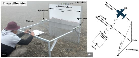
Figure 2.
(a) Pin-profilometer used to measure surface roughness in the field. (b) schematic on the top right illustrates the acquisition direction of the Sentinel-1 satellite sensor. Surface roughness is measured in the field by keeping the profile-meter parallel to the direction of the satellite.
In the field, we used the random grid sampling approach to measure the in-situ surface roughness. We divided the study area into several square grids of size 4 km × 4 km each (Figure 1). The circles marked in different colors (Figure 1) represent an average surface roughness value from 3 to 5 sampling sites (within a pixel size of the Sentinel-1) that are separated at least 20 m from each other. This is done to incorporate the effect of any spatial heterogeneity (variation) present at the length scale of a two-dimensional satellite pixel (i.e., 60 m). This minimises the measurement uncertainty and enables direct point-to-pixel comparison for training and testing the machine learning model [64,65]. Further, to measure surface roughness, we placed the pin-profiler at the location on the ground where surface roughness has to be recorded. We leveled the instrument properly using spirit levels on the two arms and on the top of the whiteboard to avoid any unintentional tilt (Figure 2a). While conducting measurements, we ensure that the pin-profiler is placed parallel to the acquisition direction of the Sentinel-1 satellite (Figure 2b). This ensures that we are measuring the same surface that is illuminated and recorded by the satellite sensors. This process ensures the qualitative measurements of surface roughness in terms of measurement directions. We have reported the directions for all the in-situ sites in Table A1. Once the instrument is laid over the surface, the pins are gently released until they touch the top surface. We take photographs by keeping the camera horizontal at the frame arm located in front of the whiteboard to capture the undulation of the pin’s position. We record the coordinates (latitude and longitude) at each sampling location using a Garmin-64s handheld GPS. At each sampling location, we have also measured the surface soil moisture using TDR-Probe (Theta-Probe). Before taking the measurements, we have calibrated the Theta-Probe (ML3 sensor) for our field using the procedure described in Singh et al. [56].
We then process the photograph that was automatically taken to detect surface roughness in MATLAB® considering the red tip of the pin as a reference (Figure 3). In doing so, we first calibrate the image to its natural size using the scale embedded on the instrument. We identify the red tips of the pins and digitise them. Once the photographs are processed, we compute the RMS surface roughness according to:
where is the number of vertical pins, is the recorded height of pin, and is the average height. The average values of the surface roughness and measurement directions are listed in Table A1 (Appendix A). Additionally, based on these values, we have classified the roughness into four major classes on the Kosi fan: stubble field, harrowed field, ploughed field, and furrow field (Figure 4).
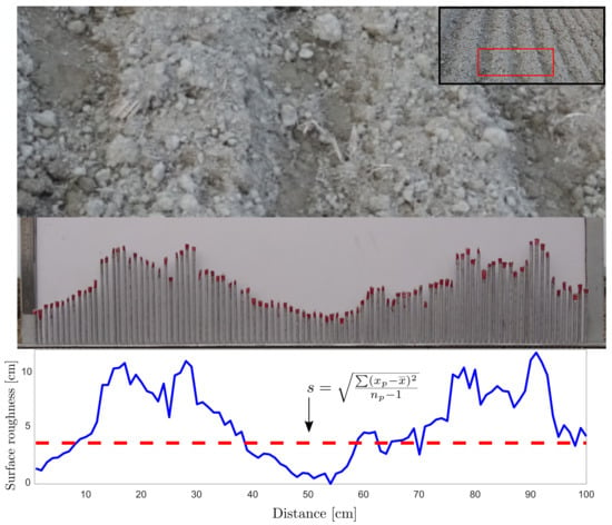
Figure 3.
Surface undulation profile extracted after processing the photographs captured for the pin-profile using a digital camera in the field.
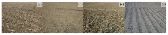
Figure 4.
Field photographs to illustrate the surface roughness conditions in different agricultural plots on the Kosi Fan. (a) shows the photograph of a stubble field (), (b) harrow field (), (c) ploughed field (), and (d) furrow field ().
3.3. Support Vector Regression
We use SVR algorithms to estimate soil roughness from satellite images. We preferred the interpretable regression-based machine-learning algorithms over the black-box models [66]. In black-box machine learning models, the prediction processes are not clear, whereas in the interpretable models, it is clear how predictions are made. Recently, the use of interpretable models has increased in machine learning [67].
The objective of a regression-based machine learning model is to obtain mapping functions that can predict the response variables. Parameters of such mapping functions are obtained from the training data. They are the initial data used to train the algorithms by fitting and tuning the parameters of a mapping function. This is usually complemented by a set of unseen datasets called the testing data and used to validate the trained machine-learning model. The SVR models are widely used to solve various problems in earth sciences, such as real-time flood stage forecasting, snow-depth retrieval, drought prediction, and landuse/landcover change analysis [68,69,70,71,72,73,74,75,76]. The SVR has an excellent generalisation capability with optimal accuracy that makes it applicable to the solution of various problems in earth sciences, image processing, wireless sensor networks, and blockchain [77,78,79,80].
Vapnik [81] introduced the support vector machine in statistical learning theory. Support vectors that deal with the regression are known as support vector regression [82]. A mathematical explanation of the SVR is provided below.
Given a sample set, S = [(,), (,), ..., (,), ..., (,)], where is the N-dimensional input data, is the corresponding output variable, and N is the total samples. Using SVR, we can estimate the dependent variable, for a given independent variable, x, according to Equation (2);
where is the high-dimensional feature spaces that are non-linearly mapped with respect to the independent variable, x. The coefficients w and b are the weight vector and bias term, respectively. The value of w and b are obtained by minimisation of the empirical risk function according to Equation (3):
where is the loss function (Figure 5b) given by;
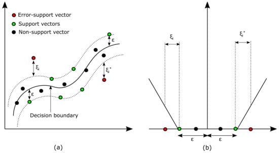
Figure 5.
Schematic to illustrate (a) the conceptual structure of the support vector regression, (b) the loss function.
The risk function (Equation (3)) is modified by introducing the relaxation variables and according to:
where is the loss factor and C is the penalty factor. To extend the SVR for non-linear function (Figure 5a), the risk function and its constraints can be rewritten in their dual form by introducing the dual set of variables using the Lagrange function.
where and are the Lagrange multipliers and K is the kernel function given according to;
We used the Homogeneous Polynomial kernel because it is a non-stationary kernel that is well-suited to standardised training data.
where and d represent the structural parameter and degree of the Polynomial function respectively.
The final risk function for the non-linear SVR reads;
3.3.1. Model Setup
We setup the SVR model to estimate surface roughness. This includes feature generation from the input features, selection of training and validation data, optimisation of the training model, and finally, model evaluation. A detailed flow chart of the model setup is illustrated in Figure 6.
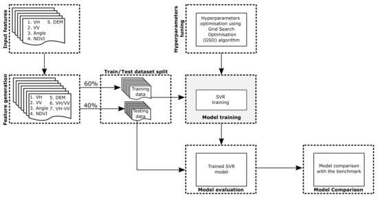
Figure 6.
Flowchart illustrates the overall methodology used to set-up the SVR model.
We identified five input features, namely incidence angle, backscatter values () Sentinel-1 for both (VH and VV) polarisation, NDVI from Sentinel-2, and elevation from the SRTM DEM. The spatial resolution of these features are different, for example; spatial resolution of the processed backscatter value () of the Sentinel-1 image is available at , NDVI at , and the surface elevation at . We applied the nearest-neighbor algorithm to resample the NDVI and elevation grids at ; a grid size comparable to the backscatter images. Finally, these input features were used to train the model and predict surface roughness. We evaluated the in-sample error (i.e., MSE) in the input features. They constitute an in-sample error of about . Furthermore, from a linear combination/fusion of input features, we generated two more features by taking the ratio of VH/VV and difference of VH–VV polarisation [83]. All seven features together reduce the in-sample error (MSE) to .
Now, we individually evaluate the relative importance of input features through regression tree ensemble in the prediction of surface roughness. We applied the Least-Squares Boosting (LSBoost) ensemble aggregation method with tree learner for 100 learning cycles to train the regression ensemble. We then calculated the predictor importance by adding changes in the MSE (created due to a split in the tree learner) and normalised it using the total branch nodes. The higher value of this ratio corresponds to high importance for the ensemble. Furthermore, we estimated predictive measures of association (i.e., feature association matrix) through Pearson’s linear correlation approach. The input features of a machine learning model should not be highly correlated. This makes the machine learning models unstable and highly sensitive [84].
We applied the Principal Component Analysis (PCA) to select the most uncorrelated information from the feature data. We selected the first five principal components of the feature data. This explains about 99% variance and reduces the time and space complexity required for the training and evaluation of the model. We then standardised the features to find the optimal scaling methods to predict surface roughness. We applied different methods, i.e., Not Standardised (NS), Center Mean (CM), Z-score Mean (ZM), Min–Max (MM), and Scale (S), to standardise our input features. Table 2 reports the description of different standardisation methods.
Table 2.
Different scaling methods and their descriptions.
Finally, we use the result of each standardisation method (i.e., PCA-NS-SVR, PCA-CM-SVR, PCA-ZM-SVR, PCA-MM-SVR, and PCA-S-SVR) to train the SVR model (Figure 7).
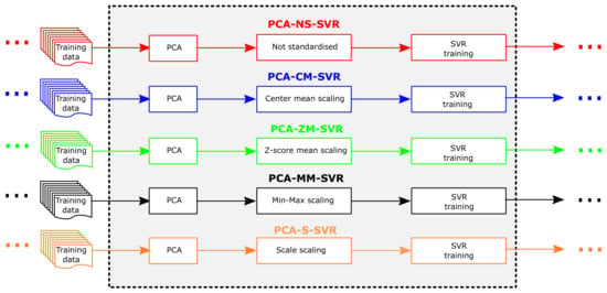
Figure 7.
SVR variants based on dimension reduction and scaling.
3.3.2. Hyperparameter Optimisation
The hyperparameters ( and C) of the SVR model determine the predictive efficiency and training error in the model. A condition where the overall residual is greater than , the hyperparameter C penalises the model output. A lower value of C results in computational complexity and a higher value of C in model under-fitting. To overcome these problems, we use the universal grid search algorithm to optimise the hyperparameter (C) by keeping the fixed in the SVR model. The Gird search algorithm needs an objective function to estimate the optimal value of the hyperparameter. In a regression model, the MSE is the most commonly used objective function [85]. The objective function (MSE) reads;
where n is the size of testing samples, is the observed values, is the predicted values. The grid search algorithm minimises the objective function to find the optimal value of C. Table 3 reports the optimal values of hyperparameters.
Table 3.
Simulation parameters of the SVR model.
4. Result
4.1. Feature Importance
The bar plot (Figure 8a) shows relative importance of our input features. A feature that has higher relative importance score is considered more important in the model for predicting surface roughness.

Figure 8.
(a) Bar plot illustrates the relative feature importance score of the input features, (b) feature association matrix.
Among all the input features we used for training SVR models, the incidence angle has the lowest, and DEM has the highest feature importance score. This indicates incidence angle has less impact, and DEM has more impact in predicting the surface soil roughness. Additional features (VH/VV and VH–VV) generated from the linear data fusion have more importance than the native features. It is important to highlight that the feature importance only calculates the relative importance, without the segregation of irrelevant and relevant features [86]. It is a common practice in machine learning to eliminate noisy, redundant, and irrelevant features, as they can reduce the prediction accuracy and increase the computational cost.
We applied the backward elimination to identify the irrelevant features in our model [87,88,89,90,91]. It is an iterative approach that eliminates the least important features and re-calculates the model loss (i.e., MSE) in each iteration. If the model loss for a feature decreases, we consider that feature irrelevant and eliminate it from the computation. This process continues until the model loss is constant. Alternatively, if the model loss increases, that feature is relevant and the process is terminated. As the incidence angle has the least feature importance score, we eliminated it using the backward elimination approach and re-calculated the model loss. We observed that, after the elimination of incidence angle, the model loss increased (MSE = ). This indicates that the incidence angle is not an irrelevant feature in the prediction of soil roughness. Similarly, the elimination of other features degrades the result. This suggests that all seven features are relevant in predicting surface soil roughness. Among them, DEM is the most important. Figure 8b shows the Pearson correlations of the features. All the input features are uncorrelated, which suggests the good reliability of our model.
4.2. Feature Sensitivity
Feature importance does not examine if a feature is positively or negatively affecting the models. To evaluate this, we performed a sensitivity analysis of our features when predicting the surface roughness. We generated the Partial Dependence Plot (PDP) [92] of each feature with their corresponding histogram (Figure 9). PDP measures the average marginal effect of all features on the predicted variable. The PDP of DEM shows a high partial dependency for surface roughness (Figure 9). The incidence angle and DEM are positive, whereas the NDVI has a negative effect on the surface roughness. The backscatter values () for VV and VH/VV have a fluctuating positive, and VH–VV has a fluctuating negative effect. We did not observe any clear trend for VH.

Figure 9.
PDP and ICE plot to show the sensitivity of different input features (i.e.; (a) VH, (b) VV, (c) VH/VV, (d) VH–VV, (e) incidence angle, (f) NDVI, and (g) DEM) on surface roughness. Curves in red and gray illustrate the PDP and ICE respectively. The corresponding histograms illustrate the probability distribution of the individual features and surface roughness.
Furthermore, to explore the localised explanation of individual features at each instance, we plotted the Individual Conditional Expectation (ICE) in the same plot [93]. This is considered a non-linear sensitivity analysis that disaggregates the averaging effects and evaluates the model at each instance. The average of all the ICE lines provides the PDP plot [94,95,96]. The averaging effect of PDP conceals any heterogeneous relationship present at any particular instance. For example, some instances in the ICE of DEM (between 50 and 55 m) behave differently compared to the majority instances (i.e., PDP).
4.3. Surface Roughness
We used the different variants of our SVR model to estimate surface roughness and compared the result with the ground measurement. We plot the model surface roughness against the in-situ values (Figure 10). We observed that the PCA-MM-SVR outperforms all other variants of SVR, with R = 0.75 and RMSE = 0.19 cm (Figure 10). The predicted surface roughness from PCA-MM-SVR accord well with the in-situ values. All the datapoints are clustered around the 1:1 line. The result of PCA-CM-SVR also compares well with the ground measurement. This ranks second-best in predicting the surface roughness with R = 0.70 and RMSE = 0.25 cm. The non-standardise version of SVR (PCA-NS-SVR) poorly performs with R = 0.50 and RMSE = 0.44 cm. This is primarily because PCA-NS-SVR underestimates the surface roughness value, and the datapoints are non-uniformly distributed on a 1:1 line with large scattering. This indicates bias in the prediction.

Figure 10.
Predicted surface roughness against the in-situ measurement. Symbols in different colours and shape illustrate the different variants of SVR models used for the prediction.
5. Discussion
5.1. Comparison with the Benchmark Machine Learning Models
Our results show that the PCA-MM-SVR predicts surface soil roughness more accurately compared to the other variants of SVR models. However, any conclusion based solely on a comparison of the different variants of the same machine-learning model may lead to a biased result. To overcome this, we compare the performance of the SVR model with the benchmark machine-learning algorithms (i.e., GPR, GRNN, BDT, Bragging Ensemble Learning, and Boosting Ensemble Learning). Apart from these benchmark algorithms, we also compared the performance of the SVR models with the recently emerged automated machine learning (AutoML) algorithms [97]. An AutoML module is embedded in MATLAB® and can be accessed through fitrauto library. It automatically selects the regression model (i.e., SVR, GPR, linear regression, BDT, and ensemble learning) with optimised hyperparameters. This uses Bayesian optimisation to iteratively tune the model through parallel computing by assuming as an objective function.
In machine learning, it is customary to use R and RMSE values to evaluate the model performance. These metrics are suitable for estimating the accuracy of a single model, but not for comparing the performance of different machine-learning models [98,99,100]. To ensure a fair evaluation, we use performance metrics such as: Akaike’s Information Criterion (AIC), corrected AIC (AICc), and Bayesian Information Criterion (BIC) [101] (Appendix B). These metrics penalise the model for a higher number of model parameters to select the best model [102,103]. The model with a lower value of AIC, AICc, and BIC is preferred.
Table 4 reports the performance of other machine learning models, evaluated using the same training and testing datasets. The SVR performs relatively well compared to the other machine-learning models. The PCA-MM-SVR exhibits the lowest values of AIC, and BIC amongst all other methods; this indicates the best goodness-of-fit. We also evaluate the model performance in terms of computational time complexity (using CPU @ 3.3 GHz, 10 cores). We observed that the computational time complexity of PCA-MM-SVR is optimal. The time complexity of the non-standardised variant of SVR (i.e., PCA-NS-SVR) is relatively high.
Table 4.
Comparison of SVR model with the benchmark machine-learning algorithms.
Other than SVR, the GRNN performs well and ranks second in terms of performance evaluation. In GRNN, the mix–max scaling variant (i.e., PCA-MM-GRNN) performs better (R = 0.67, RMSE = 0.04 cm, AIC = 509.3, AICc = −356.7, and BIC = 1241). This model is computationally more efficient than its other variants. Among the AutoML variants, we found that PCA-ZM-AutoML ranks third in terms of performance evaluation by outperforming all other variants, with R = 0.59, RMSE = 0.20 cm, AIC = 291.05, AICc = −225.70, and BIC = 784.04. We observed that the time complexity of mix–max and non-standardised scaling variant behave in a similar way for all the machine-learning models. The performance of mix–max scaling is the best in terms of computational time complexity and relatively low for the non-standardised scaling.
5.2. Comparison with Backscatter Models
We also compared the PCA-MM-SVR model’s result with the different empirical, semi-empirical backscatter, and regression models. We applied modified Dubois, modified Oh 2002, and modified Oh 2004 models [28,29,30] to estimate the surface roughness of the Kosi Fan from dual polarised Sentinel-1 images [56,104,105]. We inverted these models to obtain surface roughness from single co-polarised (i.e., VV) and single cross-polarised images (i.e., VH), and in-situ soil moisture. The inversion of different backscatter models is explained in Appendix C. Surface roughness can be estimated from SAR images by using calibrated regression curves. For example, Srivastava et al. [43] have proposed that the empirical coefficients of the linear regression model retrieve surface roughness for the Indian soils from the multi-polarized Envisat-1 ASAR images. We use this regression model to estimate the surface soil roughness of the Kosi Fan.
The surface roughness from backscatter and regression models is subjected to systematic errors and model biases. To obtain a fair comparison between the SVR, backscatter, and regression models, we use un-bias RMSE (ubRMSE) instead of RMSE. Table 5 reports a comparison of modelled surface roughness with the ground measurements.
Table 5.
Comparison of soil moisture estimated from SVR with the result of different backscatter and empirical regression models.
Among all the models discussed above, the PCA-MM-SVR machine learning performs better (R = 0.75, ubRMSE = 0.08 , and MSE = 0.04 ). The accuracy of SVR is relatively high compared to the backscatter and regression models. This is probably because the SVR considers a higher number of input features to predict the soil roughness as compared to the backscatter and regression-based models.
5.3. Surface Roughness of the Kosi Fan
Finally, we used the PCA-MM-SVR model to predict the surface roughness of the Kosi Fan for two consecutive satellite passes (11–12 and 17–18 December 2019) of the Sentinel-1. Figure 11 shows the spatial and temporal variation in surface roughness and its anomaly on the Kosi Fan Surface. The time difference between the two consecutive passes of Sentinel-1 A and B satellites is six days; we do not expect much change in the surface roughness. This is clearly reflected by the cross-section profiles drawn at a common region of the surface roughness maps of two different dates (Figure 11). We observed the negative surface roughness anomalies where surface roughness values were less than 1.5 cm and positive anomalies where the surface roughness values were greater than 1.5 cm.

Figure 11.
Spatial distribution of surface roughness predicted from PCA-MM-SVR (top) and the corresponding anomaly (bottom). The anomaly is calculated by subtracting the surface roughness at each pixel with the mean surface roughness value of the entire fan. The pixels in white represent invalid regions.
Interestingly, we observed some spatial patterns in the surface roughness of the Kosi Fan. Visually, it appears that the surface roughness is high near the apex of the fan and decreases towards the toe. Based on the elevation variation, we categorised the fan surface into proximal (110–70 m), middle (70–50 m), and distal (50–30 m) part. We drew the surface roughness profile along a longitudinal transect from the apex to the fan toe (Figure 12). We can clearly see that the surface decreases non-linearly (approximated using a nonlinear second-order polynomial equation) along the transect. The histogram of surface roughness in the proximal, middle, and distal parts appears to be normally distributed. We found a mild decrease in the average surface roughness from the proximal ( cm), middle ( cm), to the distal ( cm) part of the Kosi Fan. This is consistent with the values measured in the field. Further, it is important to note, on the Kosi fan, that the elevation (110–30 m) and median grain size (300–100 m) gradually decreases from the proximal to distal part. This indicates a possible control of the grain size of the soil sediments and elevation on the surface roughness.
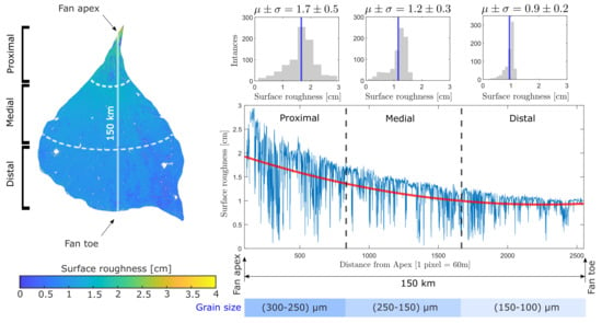
Figure 12.
Surface roughness variation from the proximal to distal part of the Kosi fan. The graph in the bottom right illustrates the surface roughness against the distance from fan apex to the toe. Histograms show the corresponding distribution of surface roughness in the proximal, middle and distal parts of the Kosi Fan.
Further, we observed that the dependency of the surface soil roughness on different features is highly dynamic and unclear. We observed no clear trend between the surface soil roughness and the features (Figure 9). However, an overall trend (or impact) is visible, with few features. For example, we observed a positive impact of DEM and incidence angle with the surface soil roughness. This observations are in consistent with the recent studies [40,106].
5.4. Sensitivity Analysis
Finally, we performed a sensitivity analysis of the PCA-MM-SVR machine learning model to assess the impact of individual features on the surface soil roughness. At every iteration, we estimated surface roughness by introducing a small uncertainty ( and ) in any one input feature at a particular time and keeping the remaining features constant. This was carried out for all the input features and the results were compared. We observed that an introduction of errors in the input features of the PCA-MM-SVR model resulted in an approximately change in the output (Figure 13).
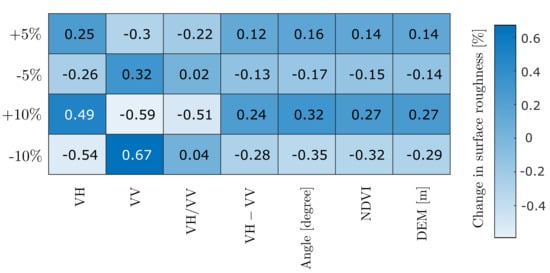
Figure 13.
Heat map illustrates the the sensitivity of the PCA-MM-SVR model for +5%, −5%, +10%, and −10% uncertainty in the input features.
6. Conclusions
We compared the accuracy of surface roughness estimated from SVR models with six different benchmark machine-learning algorithms (i.e., GPR, GRNN, BDT, BAGG, BOOST, and AutoML) and three backscatter models (modified Dubois, modified Oh 2002, and modified Oh 2004). We conclude that the PCA-MM-SVR model outperforms all the different variants of SVR, different benchmark machine learning, backscatter, and empirical regression models in terms of accuracy and computational time complexity. The PCA-MM-SVR model is relatively more sensitive to uncertainly in the VV polarisation as compared to the other input features. On the Kosi Fan, the surface roughness appears to be more in the proximal and decreases gradually towards the distal part of the fan. Although it is not clear at this stage, we suspect that this could be associated with the elevation (110–30 m) and median grain size variation (300–100 m) from proximal to the distal part of the fan.
This study provides a robust approach to estimate surface soil roughness from optical and SAR remote-sensing data. A comprehensive work using multiple SAR sensor data fusion may be examined in the future to assess the prediction of surface roughness using different machine-learning models. The result of this study can be used in various applications, such as: to study soil erosion, surface soil moisture, infiltration, overland flow, sediment detachment, and many other applications in earth sciences.
Author Contributions
A.S.: Conceptualization, Methodology, Software, Validation, Formal analysis, Writing—Original Draft Preparation, Visualization. K.G.: Conceptualization, Methodology, Software, Validation, Formal Analysis, Writing—Original Draft, Visualization, Supervision, Funding Acquisition. A.K.R. and Z.B. have contributed in the data collection in the field. All authors have read and agreed to the published version of the manuscript.
Funding
This research was funded by the Space Applications Centre (SAC-ISRO) under the NASA-ISRO Synthetic Aperture Radar (NISAR) mission through grant Hyd-01.
Institutional Review Board Statement
Not applicable.
Informed Consent Statement
Not applicable.
Data Availability Statement
All the satellite images used in this study are publicly available. We have provided the in-situ measurements in Table A1. The algorithms used in this study can be made available upon a reasonable request to the corresponding and first author.
Acknowledgments
We acknowledge IISER Bhopal for providing institutional supports. We are thankful to the Space Applications Centre, Ahmadabad (SAC-ISRO) for providing research grant (grant no: Hyd-01) under the NASA-ISRO Synthetic Aperture Radar (NISAR) mission. Abhilash Singh would like to acknowledge the Department of Science and Technology (DST), Government of India for providing funding to pursue PhD through the DST-INSPIRE fellowship (grant no. DST/INSPIRE Fellowship/IF180001) scheme. We would also like to acknowledge Gaurav Kailash Sonkar and Jitendra Kumar for their extended support during the field work. We are thankful to the editor and all the four anonymous reviewers for their comments and suggestions.
Conflicts of Interest
The authors declare no conflict of interest.
Appendix A
Surface roughness measurements on the Kosi Fan (Table A1).
Table A1.
Details of the ground condition and surface roughness measured in the field.
Table A1.
Details of the ground condition and surface roughness measured in the field.
| Site ID | Longitude | Latitude | Date dd-mm-yyyy) | Mission Identifier | Surface Roughness (cm) | Lobe | Direction | Soil Temperature (°C) | Landuse | Training/Testing |
|---|---|---|---|---|---|---|---|---|---|---|
| 01 | 86.63923 | 26.13257 | 11 December 2019 | S1A | 2.4029 | I | NE | 21 | Uncultivated bare land (Ploughed) | Training |
| 02 | 86.64361 | 26.10979 | 11 December 2019 | S1A | 1.2736 | I | NE | 22 | Uncultivated bare land (Harrowed) | Training |
| 03 | 86.62364 | 26.09691 | 11 December 2019 | S1A | 2.4072 | I | SW | 20 | Uncultivated bare land (Ploughed) | Training |
| 04 | 86.62604 | 26.0954 | 11 December 2019 | S1A | 1.5181 | I | NE | 16 | Uncultivated bare land (Harrowed) | Training |
| 05 | 86.62061 | 26.0632 | 11 December 2019 | S1A | 3.0288 | I | NE | 16 | Uncultivated bare land (Ploughed) | Training |
| 06 | 86.566 | 26.0243 | 11 December 2019 | S1A | 1.5175 | I | NE | 18 | Uncultivated bare land (Harrowed) | Training |
| 07 | 86.57533 | 25.97547 | 11 December 2019 | S1A | 1.1172 | I | NE | 19 | Uncultivated bare land (Harrowed) | Training |
| 08 | 86.64431 | 25.99772 | 11 December 2019 | S1A | 1.9886 | I | NE | 23 | Harrowed + wheat sowed | Training |
| 09 | 86.64072 | 26.03379 | 11 December 2019 | S1A | 1.3282 | I | SW | 24 | Uncultivated bare land (Harrowed) | Training |
| 10 | 86.62675 | 26.15357 | 11 December 2019 | S1A | 3.7350 | I | SW | 17 | Furrow field | Training |
| 11 | 86.66584 | 26.19629 | 11 December 2019 | S1A | 3.8858 | I | NE | 19 | Furrow field | Training |
| 12 | 86.6998 | 26.21087 | 11 December 2019 | S1A | 1.9685 | I | NE | 20 | Uncultivated bare land (Harrowed) | Training |
| 13 | 86.73994 | 26.22444 | 11 December 2019 | S1A | 1.7677 | I | NE | 20 | Harrowed + wheat sowed | Training |
| 14 | 86.75186 | 26.23693 | 11 December 2019 | S1A | 1.8670 | I | NE | 21 | Uncultivated bare land (Harrowed) | Training |
| 15 | 86.78488 | 26.24503 | 11 December 2019 | S1A | 2.2774 | I | NE | 19 | Uncultivated bare land (Ploughed) | Training |
| 16 | 86.79723 | 26.26185 | 11 December 2019 | S1A | 2.5599 | I | SW | 20 | Uncultivated bare land (Ploughed) | Training |
| 17 | 86.80273 | 26.2389 | 11 December 2019 | S1A | 1.4094 | I | NE | 21 | Uncultivated bare land (Harrowed) | Training |
| 18 | 86.79795 | 26.20753 | 11 December 2019 | S1A | 3.6128 | I | SW | 20 | Furrow field | Training |
| 19 | 86.79031 | 26.18241 | 11 December 2019 | S1A | 3.7361 | I | NE | 20 | Furrow field | Training |
| 20 | 86.76803 | 26.1514 | 11 December 2019 | S1A | 2.3002 | I | NE | 20 | Uncultivated bare land (Ploughed) | Training |
| 21 | 86.65507 | 26.11443 | 11 December 2019 | S1A | 1.2325 | I | NE | 18 | Harrowed + wheat sowed | Training |
| 22 | 86.70612 | 26.06255 | 11 December 2019 | S1A | 1.1504 | I | NE | 21 | Harrowed + wheat sowed | Training |
| 23 | 86.73248 | 26.04625 | 11 December 2019 | S1A | 0.6181 | I | NE | 21 | Direct stubble seeding | Training |
| 24 | 86.71229 | 26.03606 | 11 December 2019 | S1A | 1.0680 | I | NE | 20 | Uncultivated bare land (Harrowed) | Training |
| 25 | 86.75741 | 26.02952 | 11 December 2019 | S1A | 3.3369 | I | NE | 20 | Uncultivated bare land (Ploughed) | Training |
| 26 | 86.75144 | 25.91161 | 11 December 2019 | S1A | 1.6568 | I | NE | 20 | Uncultivated bare land (Harrowed) | Training |
| 27 | 86.66203 | 25.86703 | 15 December 2019 | S1A | 1.0155 | I | SE | 18 | Uncultivated bare land (Harrowed) | Training |
| 28 | 86.68053 | 25.82926 | 15 December 2019 | S1A | 1.1016 | I | SE | 18 | Uncultivated bare land (Harrowed) | Training |
| 29 | 86.68639 | 25.78836 | 15 December 2019 | S1A | 1.9144 | I | NW | 18 | Uncultivated bare land (Harrowed) | Training |
| 30 | 86.6876 | 25.74611 | 15 December 2019 | S1A | 1.3448 | II | NW | 19 | Harrowed + maize sowed | Training |
| 31 | 86.71125 | 25.6878 | 15 December 2019 | S1A | 1.0688 | II | NW | 18 | Uncultivated bare land (Harrowed) | Training |
| 32 | 86.69384 | 25.70237 | 15 December 2019 | S1A | 2.2058 | I | NW | 21 | Ploughed + wheat sowed | Training |
| 33 | 86.65567 | 25.72331 | 15 December 2019 | S1A | 2.1397 | I | NW | 20 | Uncultivated bare land (Ploughed) | Training |
| 34 | 86.80625 | 25.91648 | 15 December 2019 | S1A | 1.4551 | II | NW | 18 | Harrowed + wheat sowed | Training |
| 35 | 86.93388 | 25.89581 | 15 December 2019 | S1A | 1.8875 | II | NW | 17 | Harrowed + maize sowed | Training |
| 36 | 87.00225 | 25.90533 | 15 December 2019 | S1A | 2.4824 | II | NW | 20 | Uncultivated bare land (Ploughed) | Training |
| 37 | 87.06107 | 25.90827 | 15 December 2019 | S1A | 1.2896 | II | SE | 20 | Uncultivated bare land (Harrowed) | Training |
| 38 | 87.09836 | 25.92137 | 15 December 2019 | S1A | 1.7548 | II | SE | 22 | Uncultivated bare land (Harrowed) | Training |
| 39 | 87.21534 | 25.88781 | 15 December 2019 | S1A | 1.7604 | II | SE | 22 | Uncultivated bare land (Harrowed) | Training |
| 40 | 86.6099 | 25.72783 | 17 December 2019 | S1B | 2.3510 | I | NW | 20 | Uncultivated bare land (Ploughed) | Training |
| 41 | 86.57812 | 25.7314 | 17 December 2019 | S1B | 0.9426 | I | NW | 21 | Direct stubble seeding | Training |
| 42 | 86.54615 | 25.77154 | 17 December 2019 | S1B | 1.2406 | I | NW | 20 | Uncultivated bare land (Harrowed) | Training |
| 43 | 86.52457 | 25.80515 | 17 December 2019 | S1B | 1.4675 | I | NW | 20 | Uncultivated bare land (Harrowed) | Training |
| 44 | 86.53774 | 25.85775 | 17 December 2019 | S1B | 2.1787 | I | SE | 19 | Uncultivated bare land (Ploughed) | Training |
| 45 | 86.56369 | 25.8713 | 17 December 2019 | S1B | 1.8584 | I | NW | 20 | Uncultivated bare land (Harrowed) | Training |
| 46 | 87.46254 | 25.72741 | 17 December 2019 | S1B | 0.8180 | III | NE | 17 | Direct stubble seeding | Testing |
| 47 | 87.42014 | 25.6838 | 17 December 2019 | S1B | 0.8593 | III | NE | 17 | Direct stubble seeding | Testing |
| 48 | 87.39914 | 25.64069 | 17 December 2019 | S1B | 1.2080 | III | SW | 18 | Uncultivated bare land (Harrowed) | Testing |
| 49 | 87.39871 | 25.60628 | 17 December 2019 | S1B | 1.4618 | III | NE | 21 | Uncultivated bare land (Harrowed) | Testing |
| 50 | 87.42513 | 25.61369 | 17 December 2019 | S1B | 1.3488 | III | NE | 21 | Uncultivated bare land (Harrowed) | Testing |
| 51 | 87.034 | 26.29657 | 17 December 2019 | S1B | 2.1895 | II | NE | 15 | Uncultivated bare land (Ploughed) | Testing |
| 52 | 87.475 | 25.60035 | 18 December 2019 | S1A | 1.0862 | III | SW | 20 | Uncultivated bare land (Harrowed) | Testing |
| 53 | 87.48171 | 25.59672 | 18 December 2019 | S1A | 1.1235 | III | SW | 22 | Uncultivated bare land (Harrowed) | Testing |
| 54 | 87.55177 | 25.60905 | 18 December 2019 | S1A | 1.0174 | III | SW | 20 | Uncultivated bare land (Harrowed) | Testing |
| 55 | 87.54285 | 25.62759 | 18 December 2019 | S1A | 0.9566 | III | SW | 21 | Direct stubble seeding | Testing |
| 56 | 87.53111 | 25.65317 | 18 December 2019 | S1A | 1.0716 | III | NE | 22 | Uncultivated bare land (Harrowed) | Testing |
| 57 | 87.52139 | 25.67509 | 18 December 2019 | S1A | 1.0026 | III | SW | 21 | Uncultivated bare land (Harrowed) | Testing |
| 58 | 87.51138 | 25.70004 | 18 December 2019 | S1A | 2.0085 | III | SW | 21 | Uncultivated bare land (Ploughed) | Testing |
| 59 | 87.51614 | 25.81319 | 18 December 2019 | S1A | 2.0704 | III | NE | 17 | Uncultivated bare land (Ploughed) | Testing |
| 60 | 87.52789 | 25.82046 | 18 December 2019 | S1A | 1.9143 | III | SW | 17 | Uncultivated bare land (Harrowed) | Testing |
| 61 | 87.54014 | 25.91021 | 18 December 2019 | S1A | 1.9034 | III | NE | 18 | Uncultivated bare land (Harrowed) | Testing |
| 62 | 87.51805 | 25.99278 | 18 December 2019 | S1A | 1.9106 | III | SW | 18 | Uncultivated bare land (Harrowed) | Testing |
| 63 | 87.50936 | 26.00962 | 18 December 2019 | S1A | 1.1215 | III | SW | 18 | Uncultivated bare land (Harrowed) | Testing |
| 64 | 87.46062 | 26.12101 | 18 December 2019 | S1A | 1.5554 | III | SW | 19 | Uncultivated bare land (Harrowed) | Testing |
| 65 | 87.29737 | 26.22082 | 18 December 2019 | S1A | 1.9698 | III | SW | 17 | Uncultivated bare land (Harrowed) | Testing |
| 66 | 87.27813 | 26.24172 | 18 December 2019 | S1A | 2.2836 | III | SW | 18 | Uncultivated bare land (Ploughed) | Testing |
| 67 | 87.23487 | 26.27511 | 18 December 2019 | S1A | 2.2357 | III | SW | 19 | Uncultivated bare land (Ploughed) | Testing |
| 68 | 87.2269 | 26.24339 | 18 December 2019 | S1A | 1.5040 | III | SW | 20 | Uncultivated bare land (Harrowed) | Testing |
| 69 | 87.2321 | 26.20331 | 18 December 2019 | S1A | 2.2703 | III | SW | 18 | Uncultivated bare land (Ploughed) | Testing |
| 70 | 87.23437 | 26.17834 | 18 December 2019 | S1A | 2.0355 | III | NE | 19 | Ploughed + wheat sowed | Testing |
| 71 | 87.23401 | 26.13083 | 18 December 2019 | S1A | 1.0870 | III | NE | 18 | Harrowed + wheat sowed | Testing |
| 72 | 87.25929 | 26.01328 | 18 December 2019 | S1A | 1.7560 | II | SW | 18 | Uncultivated bare land (Harrowed) | Testing |
| 73 | 87.30746 | 25.93218 | 18 December 2019 | S1A | 1.1182 | III | NE | 17 | Harrowed + maize sowed | Testing |
| 74 | 87.20622 | 26.326 | 18 December 2019 | S1A | 2.2675 | III | SW | 15 | Uncultivated bare land (Ploughed) | Testing |
| 75 | 87.00787 | 26.17258 | 20 December 2019 | S1A | 2.8180 | II | NE | 16 | Uncultivated bare land (Ploughed) | Testing |
| 76 | 86.99307 | 26.05495 | 20 December 2019 | S1A | 2.0213 | II | NE | 17 | Uncultivated bare land (Ploughed) | Testing |
| 77 | 86.97813 | 25.77722 | 20 December 2019 | S1A | 1.7262 | II | SW | 18 | Uncultivated bare land (Harrowed) | Testing |
| 78 | 86.96597 | 25.71033 | 20 December 2019 | S1A | 1.3681 | II | NE | 18 | Uncultivated bare land (Harrowed) | Testing |
Appendix B
The performance metrics are estimated according to;
where, SSE is the sum of squares of errors, SST is the sum of squares of total, is the observed or in-situ values, and is the satellite derived or predicted values.
where is the number of training samples and p is the number of parameters that the machine learning model evaluates internally.
Appendix C
Equation (A8) proposed by Dubois et al. [28] can be inverted according to (Equation (A9)) to estimate surface soil roughness (s).
where , , k, and are the wavelength, incidence angle, wave number, and soil permitivity respectively.
Equation (A10) proposed by Oh et al. [29] can be inverted according to (Equation (A11)) to estimate soil surface roughness.
where is the measured volumetric surface soil moisture (in-situ).
Equation (A12) proposed by Oh [30] can be inverted according to (Equation (A13)) to estimate surface roughness:
Linear regression model proposed by Srivastava et al. [43] can be used to estimate surface soil roughness.
where A and B are the empirical constants.
References
- McColl, K.A.; Alemohammad, S.H.; Akbar, R.; Konings, A.G.; Yueh, S.; Entekhabi, D. The global distribution and dynamics of surface soil moisture. Nat. Geosci. 2017, 10, 100–104. [Google Scholar] [CrossRef]
- Helming, K.; Römkens, M.; Prasad, S. Surface roughness related processes of runoff and soil loss: A flume study. Soil Sci. Soc. Am. J. 1998, 62, 243–250. [Google Scholar] [CrossRef]
- Wagner, W.; Blöschl, G.; Pampaloni, P.; Calvet, J.C.; Bizzarri, B.; Wigneron, J.P.; Kerr, Y. Operational readiness of microwave remote sensing of soil moisture for hydrologic applications. Hydrol. Res. 2007, 38, 1–20. [Google Scholar] [CrossRef]
- Baghdadi, N.; El Hajj, M.; Choker, M.; Zribi, M.; Bazzi, H.; Vaudour, E.; Gilliot, J.M.; Ebengo, D.M. Potential of Sentinel-1 images for estimating the soil roughness over bare agricultural soils. Water 2018, 10, 131. [Google Scholar] [CrossRef] [Green Version]
- Alexakis, D.D.; Mexis, F.D.K.; Vozinaki, A.E.K.; Daliakopoulos, I.N.; Tsanis, I.K. Soil moisture content estimation based on Sentinel-1 and auxiliary earth observation products. A hydrological approach. Sensors 2017, 17, 1455. [Google Scholar] [CrossRef] [Green Version]
- Verhoest, N.E.; Lievens, H.; Wagner, W.; Álvarez-Mozos, J.; Moran, M.S.; Mattia, F. On the soil roughness parameterization problem in soil moisture retrieval of bare surfaces from synthetic aperture radar. Sensors 2008, 8, 4213–4248. [Google Scholar] [CrossRef] [Green Version]
- Romkens, M.; Wang, J. Effect of tillage on surface roughness. Trans. ASAE 1986, 29, 429–0433. [Google Scholar] [CrossRef]
- Govers, G.; Takken, I.; Helming, K. Soil roughness and overland flow. Agronomie 2000, 20, 131–146. [Google Scholar] [CrossRef]
- Snapir, B.; Hobbs, S.; Waine, T. Roughness measurements over an agricultural soil surface with Structure from Motion. ISPRS J. Photogramm. Remote Sens. 2014, 96, 210–223. [Google Scholar] [CrossRef]
- Turner, R.; Panciera, R.; Tanase, M.A.; Lowell, K.; Hacker, J.M.; Walker, J.P. Estimation of soil surface roughness of agricultural soils using airborne LiDAR. Remote Sens. Environ. 2014, 140, 107–117. [Google Scholar] [CrossRef]
- Hamze, M.; Baghdadi, N.; El Hajj, M.M.; Zribi, M.; Bazzi, H.; Cheviron, B.; Faour, G. Integration of L-Band Derived Soil Roughness into a Bare Soil Moisture Retrieval Approach from C-Band SAR Data. Remote Sens. 2021, 13, 2102. [Google Scholar] [CrossRef]
- Thomsen, L.; Baartman, J.; Barneveld, R.; Starkloff, T.; Stolte, J. Soil surface roughness: Comparing old and new measuring methods and application in a soil erosion model. Soil 2015, 1, 399–410. [Google Scholar] [CrossRef] [Green Version]
- Saleh, A. Soil roughness measurement: Chain method. J. Soil Water Conserv. 1993, 48, 527–529. [Google Scholar]
- Hajnsek, I.; Pottier, E.; Cloude, S.R. Inversion of surface parameters from polarimetric SAR. IEEE Trans. Geosci. Remote. Sens. 2003, 41, 727–744. [Google Scholar] [CrossRef]
- Merzouki, A.; McNairn, H.; Pacheco, A. Mapping soil moisture using RADARSAT-2 data and local autocorrelation statistics. IEEE J. Sel. Top. Appl. Earth Obs. Remote Sens. 2011, 4, 128–137. [Google Scholar] [CrossRef]
- Le Morvan, A.; Zribi, M.; Baghdadi, N.; Chanzy, A. Soil moisture profile effect on radar signal measurement. Sensors 2008, 8, 256–270. [Google Scholar] [CrossRef] [Green Version]
- Zheng, X.; Li, L.; Chen, S.; Jiang, T.; Li, X.; Zhao, K. Temporal evolution characteristics and prediction methods of spatial correlation function shape of rough soil surfaces. Soil Tillage Res. 2019, 195, 104417. [Google Scholar] [CrossRef]
- Alijani, Z.; Lindsay, J.; Chabot, M.; Rowlandson, T.; Berg, A. Sensitivity of C-Band SAR Polarimetric Variables to the Directionality of Surface Roughness Parameters. Remote Sens. 2021, 13, 2210. [Google Scholar] [CrossRef]
- Gharechelou, S.; Tateishi, R.; A Johnson, B. A Simple Method for the Parameterization of Surface Roughness from Microwave Remote Sensing. Remote Sens. 2018, 10, 1711. [Google Scholar] [CrossRef] [Green Version]
- Jester, W.; Klik, A. Soil surface roughness measurement—Methods, applicability, and surface representation. Catena 2005, 64, 174–192. [Google Scholar] [CrossRef]
- Peng, J.; Albergel, C.; Balenzano, A.; Brocca, L.; Cartus, O.; Cosh, M.H.; Crow, W.T.; Dabrowska-Zielinska, K.; Dadson, S.; Davidson, M.W.; et al. A roadmap for high-resolution satellite soil moisture applications—Confronting product characteristics with user requirements. Remote Sens. Environ. 2020, 252, 112162. [Google Scholar] [CrossRef]
- Le Page, M.; Jarlan, L.; El Hajj, M.M.; Zribi, M.; Baghdadi, N.; Boone, A. Potential for the detection of irrigation events on maize plots using sentinel-1 soil moisture products. Remote Sens. 2020, 12, 1621. [Google Scholar] [CrossRef]
- Fersch, B.; Jagdhuber, T.; Schrön, M.; Völksch, I.; Jäger, M. Synergies for soil moisture retrieval across scales from airborne polarimetric SAR, cosmic ray neutron roving, and an in situ sensor network. Water Resour. Res. 2018, 54, 9364–9383. [Google Scholar] [CrossRef]
- Marzahn, P.; Rieke-Zapp, D.; Ludwig, R. Assessment of soil surface roughness statistics for microwave remote sensing applications using a simple photogrammetric acquisition system. ISPRS J. Photogramm. Remote Sens. 2012, 72, 80–89. [Google Scholar] [CrossRef]
- Panciera, R.; Walker, J.P.; Merlin, O. Improved understanding of soil surface roughness parameterization for L-band passive microwave soil moisture retrieval. IEEE Geosci. Remote Sens. Lett. 2009, 6, 625–629. [Google Scholar] [CrossRef]
- Oh, Y.; Sarabandi, K.; Ulaby, F.T. An empirical model and an inversion technique for radar scattering from bare soil surfaces. IEEE Trans. Geosci. Remote Sens. 1992, 30, 370–381. [Google Scholar] [CrossRef]
- Oh, Y.; Sarabandi, K.; Ulaby, F.T. An inversion algorithm for retrieving soil moisture and surface roughness from polarimetric radar observation. In Proceedings of the IGARSS’94-1994 IEEE International Geoscience and Remote Sensing Symposium, Pasadena, CA, USA, 8–12 August 1994; Volume 3, pp. 1582–1584. [Google Scholar]
- Dubois, P.C.; Van Zyl, J.; Engman, T. Measuring soil moisture with imaging radars. IEEE Trans. Geosci. Remote Sens. 1995, 33, 915–926. [Google Scholar] [CrossRef] [Green Version]
- Oh, Y.; Sarabandi, K.; Ulaby, F.T. Semi-empirical model of the ensemble-averaged differential Mueller matrix for microwave backscattering from bare soil surfaces. IEEE Trans. Geosci. Remote Sens. 2002, 40, 1348–1355. [Google Scholar] [CrossRef] [Green Version]
- Oh, Y. Quantitative retrieval of soil moisture content and surface roughness from multipolarized radar observations of bare soil surfaces. IEEE Trans. Geosci. Remote Sens. 2004, 42, 596–601. [Google Scholar] [CrossRef]
- Attema, E.; Ulaby, F.T. Vegetation modeled as a water cloud. Radio Sci. 1978, 13, 357–364. [Google Scholar] [CrossRef]
- Fung, A.K.; Li, Z.; Chen, K.S. Backscattering from a randomly rough dielectric surface. IEEE Trans. Geosci. Remote Sens. 1992, 30, 356–369. [Google Scholar] [CrossRef]
- Fung, A.K. Microwave Scattering and Emission Models and Their Applications; Artech House: Norwood, MA, USA, 1994. [Google Scholar]
- Shi, J.; Wang, J.; Hsu, A.; O’Neili, P.; Engman, E.T. Estimation of soil moisture and surface roughness parameters using L-band SAR measurements. In Proceedings of the 1995 International Geoscience and Remote Sensing Symposium, IGARSS’95. Quantitative Remote Sensing for Science and Applications, Firenze, Italy, 10–14 July 1995; Volume 1, pp. 507–509. [Google Scholar]
- Shi, J.; Wang, J.; Hsu, A.Y.; O’Neill, P.E.; Engman, E.T. Estimation of bare surface soil moisture and surface roughness parameter using L-band SAR image data. IEEE Trans. Geosci. Remote Sens. 1997, 35, 1254–1266. [Google Scholar]
- Baghdadi, N.; King, C.; Bourguignon, A.; Remond, A. Potential of ERS and RADARSAT data for surface roughness monitoring over bare agricultural fields: Application to catchments in Northern France. Int. J. Remote Sens. 2002, 23, 3427–3442. [Google Scholar] [CrossRef]
- Zribi, M.; Baghdadi, N.; Guérin, C. Analysis of surface roughness heterogeneity and scattering behavior for radar measurements. IEEE Trans. Geosci. Remote Sens. 2006, 44, 2438–2444. [Google Scholar] [CrossRef]
- Rahman, M.; Moran, M.; Thoma, D.; Bryant, R.; Collins, C.H.; Jackson, T.; Orr, B.; Tischler, M. Mapping surface roughness and soil moisture using multi-angle radar imagery without ancillary data. Remote Sens. Environ. 2008, 112, 391–402. [Google Scholar] [CrossRef]
- Baghdadi, N.; Cresson, R.; Hajj, M.E.; Ludwig, R.; Jeunesse, I.L. Estimation of soil parameters over bare agriculture areas from C-band polarimetric SAR data using neural networks. Hydrol. Earth Syst. Sci. 2012, 16, 1607–1621. [Google Scholar] [CrossRef] [Green Version]
- Sawada, Y.; Koike, T.; Aida, K.; Toride, K.; Walker, J.P. Fusing microwave and optical satellite observations to simultaneously retrieve surface soil moisture, vegetation water content, and surface soil roughness. IEEE Trans. Geosci. Remote Sens. 2017, 55, 6195–6206. [Google Scholar] [CrossRef]
- Mirmazloumi, S.M.; Sahebi, M.R.; Amani, M. New empirical backscattering models for estimating bare soil surface parameters. Int. J. Remote Sens. 2021, 42, 1928–1947. [Google Scholar] [CrossRef]
- Zribi, M.; Dechambre, M. A new empirical model to retrieve soil moisture and roughness from C-band radar data. Remote Sens. Environ. 2003, 84, 42–52. [Google Scholar] [CrossRef]
- Srivastava, H.; Patel, P.; Navalgund, R.; Sharma, Y. Retrieval of surface roughness using multi-polarized Envisat-1 ASAR data. Geocarto Int. 2008, 23, 67–77. [Google Scholar] [CrossRef]
- Ullmann, T.; Stauch, G. Surface Roughness Estimation in the Orog Nuur Basin (Southern Mongolia) Using Sentinel-1 SAR Time Series and Ground-Based Photogrammetry. Remote Sens. 2020, 12, 3200. [Google Scholar] [CrossRef]
- Azizi, A.; Abbaspour-Gilandeh, Y.; Mesri-Gundoshmian, T.; Farooque, A.A.; Afzaal, H. Estimation of soil surface roughness using stereo vision approach. Sensors 2021, 21, 4386. [Google Scholar] [CrossRef]
- Hsieh, C.Y.; Fung, A.K.; Nesti, G.; Sieber, A.J.; Coppo, P. A further study of the IEM surface scattering model. IEEE Trans. Geosci. Remote Sens. 1997, 35, 901–909. [Google Scholar] [CrossRef]
- Mancini, M.; Hoeben, R.; Troch, P.A. Multifrequency radar observations of bare surface soil moisture content: A laboratory experiment. Water Resour. Res. 1999, 35, 1827–1838. [Google Scholar] [CrossRef]
- Wells, N.A.; Dorr, J.A., Jr. Shifting of the Kosi river, northern India. Geology 1987, 15, 204–207. [Google Scholar] [CrossRef]
- Sinha, R. The great avulsion of Kosi on 18 August 2008. Curr. Sci. 2009, 97, 429–433. [Google Scholar]
- Sinha, R. The Kosi Megafan: The best-known Himalayan megafan. In Landscapes and Landforms of India; Springer: Dordrecht, The Netherlands, 2014; pp. 151–156. [Google Scholar]
- Gaurav, K.; Métivier, F.; Devauchelle, O.; Sinha, R.; Chauvet, H.; Houssais, M.; Bouquerel, H. Morphology of the Kosi megafan channels. Earth Surface Dyn. 2015, 3, 321–331. [Google Scholar] [CrossRef] [Green Version]
- Gaurav, K.; Tandon, S.; Devauchelle, O.; Sinha, R.; Métivier, F. A single width—Discharge regime relationship for individual threads of braided and meandering rivers from the Himalayan Foreland. Geomorphology 2017, 295, 126–133. [Google Scholar] [CrossRef] [Green Version]
- NRSC. District and Category Wise Distribution of Land Use and Land Cover in Bihar (2015–2016). ISRO; 2017. Available online: https://bhuvan.nrsc.gov.in/home/index.php (accessed on 25 March 2021).
- Singh, A.; Meena, G.K.; Kumar, S.; Gaurav, K. Analysis of the effect of incidence angle and moisture content on the penetration depth of L- and S-band SAR signals into the ground surface. ISPRS Ann. Photogramm. Remote Sens. Spat. Inf. Sci. 2018, 4, 197–202. [Google Scholar] [CrossRef] [Green Version]
- Singh, A.; Meena, G.K.; Kumar, S.; Gaurav, K. Evaluation of the Penetration Depth of L-and S-Band (NISAR mission) Microwave SAR Signals into Ground. In Proceedings of the 2019 URSI Asia-Pacific Radio Science Conference (AP-RASC), New Delhi, India, 9–15 March 2019; p. 1. [Google Scholar] [CrossRef]
- Singh, A.; Gaurav, K.; Meena, G.K.; Kumar, S. Estimation of soil moisture applying modified dubois model to Sentinel-1; a regional study from central India. Remote Sens. 2020, 12, 2266. [Google Scholar] [CrossRef]
- DeVries, B.; Huang, C.; Armston, J.; Huang, W.; Jones, J.W.; Lang, M.W. Rapid and robust monitoring of flood events using Sentinel-1 and Landsat data on the Google Earth Engine. Remote Sens. Environ. 2020, 240, 111664. [Google Scholar] [CrossRef]
- Martins, V.S.; Barbosa, C.C.F.; De Carvalho, L.A.S.; Jorge, D.S.F.; Lobo, F.d.L.; Novo, E.M.L.d.M. Assessment of atmospheric correction methods for Sentinel-2 MSI images applied to Amazon floodplain lakes. Remote Sens. 2017, 9, 322. [Google Scholar] [CrossRef] [Green Version]
- Li, J.; Roy, D.P. A global analysis of Sentinel-2A, Sentinel-2B and Landsat-8 data revisit intervals and implications for terrestrial monitoring. Remote Sens. 2017, 9, 902. [Google Scholar] [CrossRef] [Green Version]
- Jensen, J.R. Introductory Digital Image Processing: A Remote Sensing Perspective, 2nd ed.; Prentice-Hall Inc.: Hoboken, NJ, USA, 1996. [Google Scholar]
- Werner, M. Shuttle radar topography mission (SRTM) mission overview. Frequenz 2001, 55, 75–79. [Google Scholar] [CrossRef]
- Farr, T.G.; Kobrick, M. Shuttle Radar Topography Mission produces a wealth of data. Eos Trans. Am. Geophys. Union 2000, 81, 583–585. [Google Scholar] [CrossRef]
- Farr, T.G.; Rosen, P.A.; Caro, E.; Crippen, R.; Duren, R.; Hensley, S.; Kobrick, M.; Paller, M.; Rodriguez, E.; Roth, L.; et al. The shuttle radar topography mission. Rev. Geophys. 2007, 45. [Google Scholar] [CrossRef] [Green Version]
- Ryan, J.; Hubbard, A.; Irvine-Fynn, T.D.; Doyle, S.H.; Cook, J.; Stibal, M.; Box, J. How robust are in situ observations for validating satellite-derived albedo over the dark zone of the Greenland Ice Sheet? Geophys. Res. Lett. 2017, 44, 6218–6225. [Google Scholar] [CrossRef] [Green Version]
- Thakur, K.K.; Vanderstichel, R.; Barrell, J.; Stryhn, H.; Patanasatienkul, T.; Revie, C.W. Comparison of remotely-sensed sea surface temperature and salinity products with in situ measurements from British Columbia, Canada. Front. Mar. Sci. 2018, 5, 121. [Google Scholar] [CrossRef] [Green Version]
- Rudin, C. Stop explaining black box machine learning models for high stakes decisions and use interpretable models instead. Nat. Mach. Intell. 2019, 1, 206–215. [Google Scholar] [CrossRef] [Green Version]
- Murdoch, W.J.; Singh, C.; Kumbier, K.; Abbasi-Asl, R.; Yu, B. Definitions, methods, and applications in interpretable machine learning. Proc. Natl. Acad. Sci. USA 2019, 116, 22071–22080. [Google Scholar] [CrossRef] [Green Version]
- Mountrakis, G.; Im, J.; Ogole, C. Support vector machines in remote sensing: A review. ISPRS J. Photogramm. Remote Sens. 2011, 66, 247–259. [Google Scholar] [CrossRef]
- Yu, P.S.; Chen, S.T.; Chang, I.F. Support vector regression for real-time flood stage forecasting. J. Hydrol. 2006, 328, 704–716. [Google Scholar] [CrossRef]
- Xiao, X.; Zhang, T.; Zhong, X.; Shao, W.; Li, X. Support vector regression snow-depth retrieval algorithm using passive microwave remote sensing data. Remote Sens. Environ. 2018, 210, 48–64. [Google Scholar] [CrossRef]
- Kuter, S. Completing the machine learning saga in fractional snow cover estimation from MODIS Terra reflectance data: Random forests versus support vector regression. Remote Sens. Environ. 2021, 255, 112294. [Google Scholar] [CrossRef]
- Ge, J.; Meng, B.; Liang, T.; Feng, Q.; Gao, J.; Yang, S.; Huang, X.; Xie, H. Modeling alpine grassland cover based on MODIS data and support vector machine regression in the headwater region of the Huanghe River, China. Remote Sens. Environ. 2018, 218, 162–173. [Google Scholar] [CrossRef]
- Xie, X.; Liu, W.T.; Tang, B. Spacebased estimation of moisture transport in marine atmosphere using support vector regression. Remote Sens. Environ. 2008, 112, 1846–1855. [Google Scholar] [CrossRef]
- Okujeni, A.; van der Linden, S.; Tits, L.; Somers, B.; Hostert, P. Support vector regression and synthetically mixed training data for quantifying urban land cover. Remote Sens. Environ. 2013, 137, 184–197. [Google Scholar] [CrossRef]
- Su, H.; Wu, X.; Yan, X.H.; Kidwell, A. Estimation of subsurface temperature anomaly in the Indian Ocean during recent global surface warming hiatus from satellite measurements: A support vector machine approach. Remote Sens. Environ. 2015, 160, 63–71. [Google Scholar] [CrossRef]
- Malik, A.; Tikhamarine, Y.; Souag-Gamane, D.; Rai, P.; Sammen, S.S.; Kisi, O. Support vector regression integrated with novel meta-heuristic algorithms for meteorological drought prediction. Meteorol. Atmos. Phys. 2021, 133, 891–909. [Google Scholar] [CrossRef]
- Jebadurai, J.; Peter, J.D. SK-SVR: Sigmoid kernel support vector regression based in-scale single image super-resolution. Pattern Recognit. Lett. 2017, 94, 144–153. [Google Scholar] [CrossRef]
- Ni, K.S.; Nguyen, T.Q. Image superresolution using support vector regression. IEEE Trans. Image Process. 2007, 16, 1596–1610. [Google Scholar] [CrossRef]
- Peng, Y.; Albuquerque, P.H.M.; de Sá, J.M.C.; Padula, A.J.A.; Montenegro, M.R. The best of two worlds: Forecasting high frequency volatility for cryptocurrencies and traditional currencies with Support Vector Regression. Expert Syst. Appl. 2018, 97, 177–192. [Google Scholar] [CrossRef]
- Ghanem, K.; Aparicio-Navarro, F.J.; Kyriakopoulos, K.G.; Lambotharan, S.; Chambers, J.A. Support vector machine for network intrusion and cyber-attack detection. In Proceedings of the 2017 Sensor Signal Processing for Defence Conference (SSPD), London, UK, 6–7 December 2017; pp. 1–5. [Google Scholar]
- Vapnik, V.N. The Nature of Statistical Learning Theory; Springer: New York, NY, USA, 1995. [Google Scholar]
- Drucker, H.; Burges, C.J.; Kaufman, L.; Smola, A.J.; Vapnik, V. Support vector regression machines. In Advances in Neural Information Processing Systems; Denver, CO, USA, December 1997; pp. 155–161. Available online: https://papers.nips.cc/paper/1996/file/d38901788c533e8286cb6400b40b386d-Paper.pdf (accessed on 13 July 2021).
- Ittner, A.; Schlosser, M. Discovery of Relevant New Features by Generating Non-Linear Decision Trees. In Proceedings of the Second International Conference on Knowledge Discovery and Data Mining, Portland, OR, USA, 2–4 August 1996; pp. 108–113. [Google Scholar]
- Toloşi, L.; Lengauer, T. Classification with correlated features: Unreliability of feature ranking and solutions. Bioinformatics 2011, 27, 1986–1994. [Google Scholar] [CrossRef] [PubMed]
- Reed, R.; MarksII, R.J. Neural Smithing: Supervised Learning in Feedforward Artificial Neural Networks; MIT Press: Cambridge, MA, USA, 1999. [Google Scholar]
- Tuv, E.; Borisov, A.; Runger, G.; Torkkola, K. Feature selection with ensembles, artificial variables, and redundancy elimination. J. Mach. Learn. Res. 2009, 10, 1341–1366. [Google Scholar]
- Kohavi, R.; Sommerfield, D. Feature Subset Selection Using the Wrapper Method: Overfitting and Dynamic Search Space Topology. 1995, pp. 192–197. Available online: https://www.aaai.org/Papers/KDD/1995/KDD95-049.pdf (accessed on 13 July 2021).
- John, G.H.; Kohavi, R.; Pfleger, K. Irrelevant features and the subset selection problem. In Machine Learning Proceedings 1994; Morgan Kaufmann Publishers: San Francisco, CA, USA, 1994; pp. 121–129. [Google Scholar]
- Kohavi, R.; John, G.H. Wrappers for feature subset selection. Artif. Intell. 1997, 97, 273–324. [Google Scholar] [CrossRef] [Green Version]
- Mao, K.Z. Orthogonal forward selection and backward elimination algorithms for feature subset selection. IEEE Trans. Syst. Man Cybern. Part B (Cybernetics) 2004, 34, 629–634. [Google Scholar] [CrossRef]
- Pham, B.T.; Nguyen-Thoi, T.; Ly, H.B.; Nguyen, M.D.; Al-Ansari, N.; Tran, V.Q.; Le, T.T. Extreme learning machine based prediction of soil shear strength: A sensitivity analysis using Monte Carlo simulations and feature backward elimination. Sustainability 2020, 12, 2339. [Google Scholar] [CrossRef] [Green Version]
- Friedman, J.H. Greedy function approximation: A gradient boosting machine. Ann. Stat. 2001, 29, 1189–1232. [Google Scholar] [CrossRef]
- Goldstein, A.; Kapelner, A.; Bleich, J.; Pitkin, E. Peeking inside the black box: Visualizing statistical learning with plots of individual conditional expectation. J. Comput. Graph. Stat. 2015, 24, 44–65. [Google Scholar] [CrossRef]
- Ly, H.B.; Le, T.T.; Vu, H.L.T.; Tran, V.Q.; Le, L.M.; Pham, B.T. Computational hybrid machine learning based prediction of shear capacity for steel fiber reinforced concrete beams. Sustainability 2020, 12, 2709. [Google Scholar] [CrossRef] [Green Version]
- Singh, A.; Kotiyal, V.; Sharma, S.; Nagar, J.; Lee, C.C. A machine learning approach to predict the average localization error with applications to wireless sensor networks. IEEE Access 2020, 8, 208253–208263. [Google Scholar] [CrossRef]
- Singh, A.; Nagar, J.; Sharma, S.; Kotiyal, V. A Gaussian process regression approach to predict the k-barrier coverage probability for intrusion detection in wireless sensor networks. Expert Syst. Appl. 2021, 172, 114603. [Google Scholar] [CrossRef]
- He, X.; Zhao, K.; Chu, X. AutoML: A Survey of the State-of-the-Art. Knowl. Based Syst. 2021, 212, 106622. [Google Scholar] [CrossRef]
- Neill, S.P.; Hashemi, M.R. Fundamentals of Ocean Renewable Energy: Generating Electricity from the Sea; Academic Press; Elsevier Ltd., 2018; Available online: https://www.elsevier.com/books/fundamentals-of-ocean-renewable-energy/neill/978-0-12-810448-4 (accessed on 13 July 2021).
- Botchkarev, A. Performance metrics (error measures) in machine learning regression, forecasting and prognostics: Properties and typology. arXiv 2018, arXiv:1809.03006. [Google Scholar]
- Yang, Y.; Ye, Z.; Su, Y.; Zhao, Q.; Li, X.; Ouyang, D. Deep learning for in vitro prediction of pharmaceutical formulations. Acta Pharm. Sin. B 2019, 9, 177–185. [Google Scholar] [CrossRef]
- Pham, H. A new criterion for model selection. Mathematics 2019, 7, 1215. [Google Scholar] [CrossRef] [Green Version]
- Vrieze, S.I. Model selection and psychological theory: A discussion of the differences between the Akaike information criterion (AIC) and the Bayesian information criterion (BIC). Psychol. Methods 2012, 17, 228. [Google Scholar] [CrossRef] [Green Version]
- Claeskens, G.; Hjort, N.L. Model Selection and Model Averaging, Cambridge Books; Cambridge University Press: Cambridge, UK, 2008; number 9780521852258, 1-312; Available online: https://ideas.repec.org/b/cup/cbooks/9780521852258.html (accessed on 13 July 2021).
- Rao, S.S.; Das, S.; Nagaraju, M.; Venugopal, M.; Rajankar, P.; Laghate, P.; Reddy, M.S.; Joshi, A.; Sharma, J. Modified Dubois model for estimating soil moisture with dual polarized SAR data. J. Indian Soc. Remote Sens. 2013, 41, 865–872. [Google Scholar]
- Choker, M.; Baghdadi, N.; Zribi, M.; El Hajj, M.; Paloscia, S.; Verhoest, N.E.; Lievens, H.; Mattia, F. Evaluation of the Oh, Dubois and IEM backscatter models using a large dataset of SAR data and experimental soil measurements. Water 2017, 9, 38. [Google Scholar] [CrossRef]
- Zhu, L.; Walker, J.P.; Ye, N.; Rüdiger, C. Roughness and vegetation change detection: A pre-processing for soil moisture retrieval from multi-temporal SAR imagery. Remote Sens. Environ. 2019, 225, 93–106. [Google Scholar] [CrossRef]
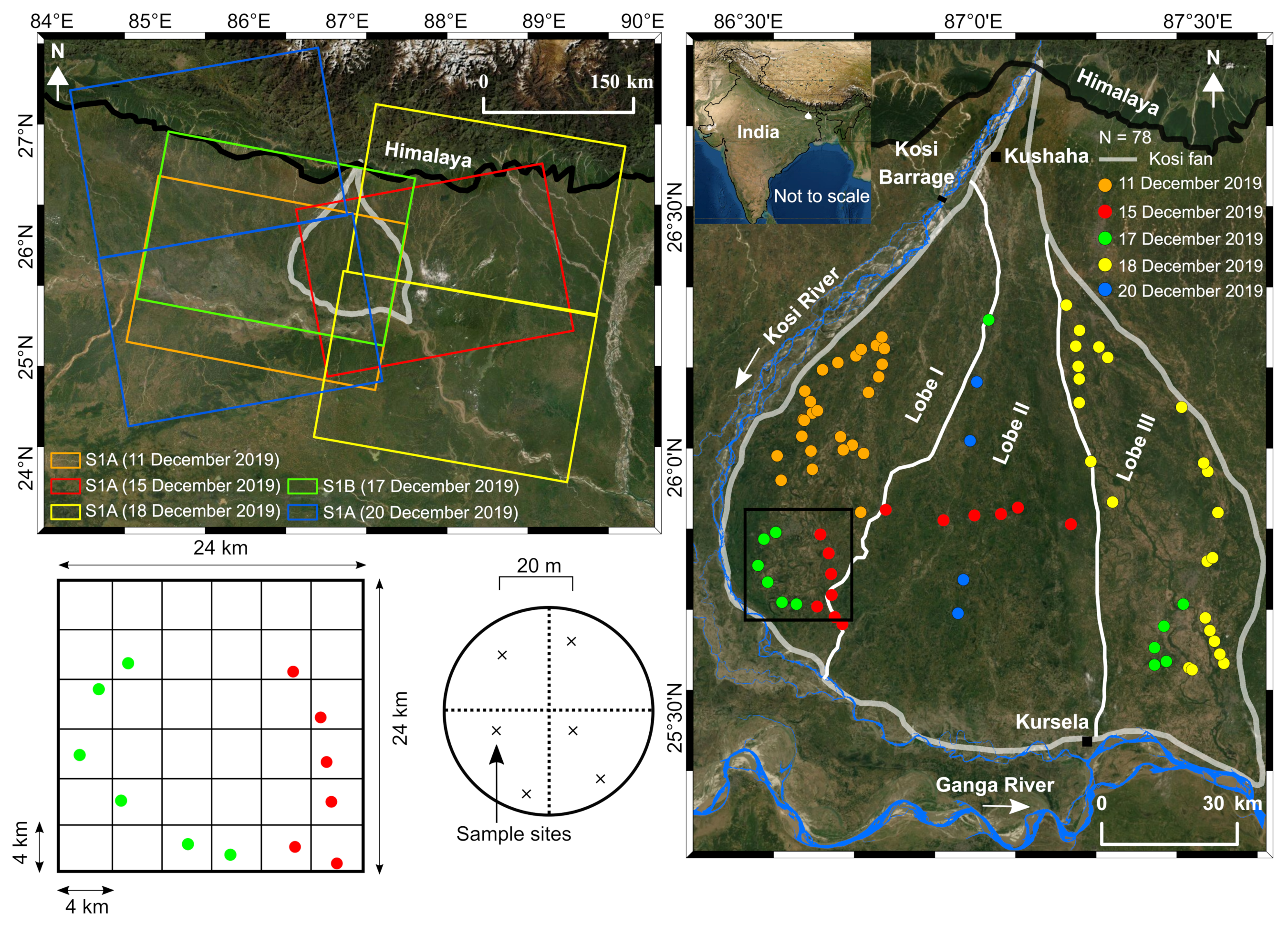

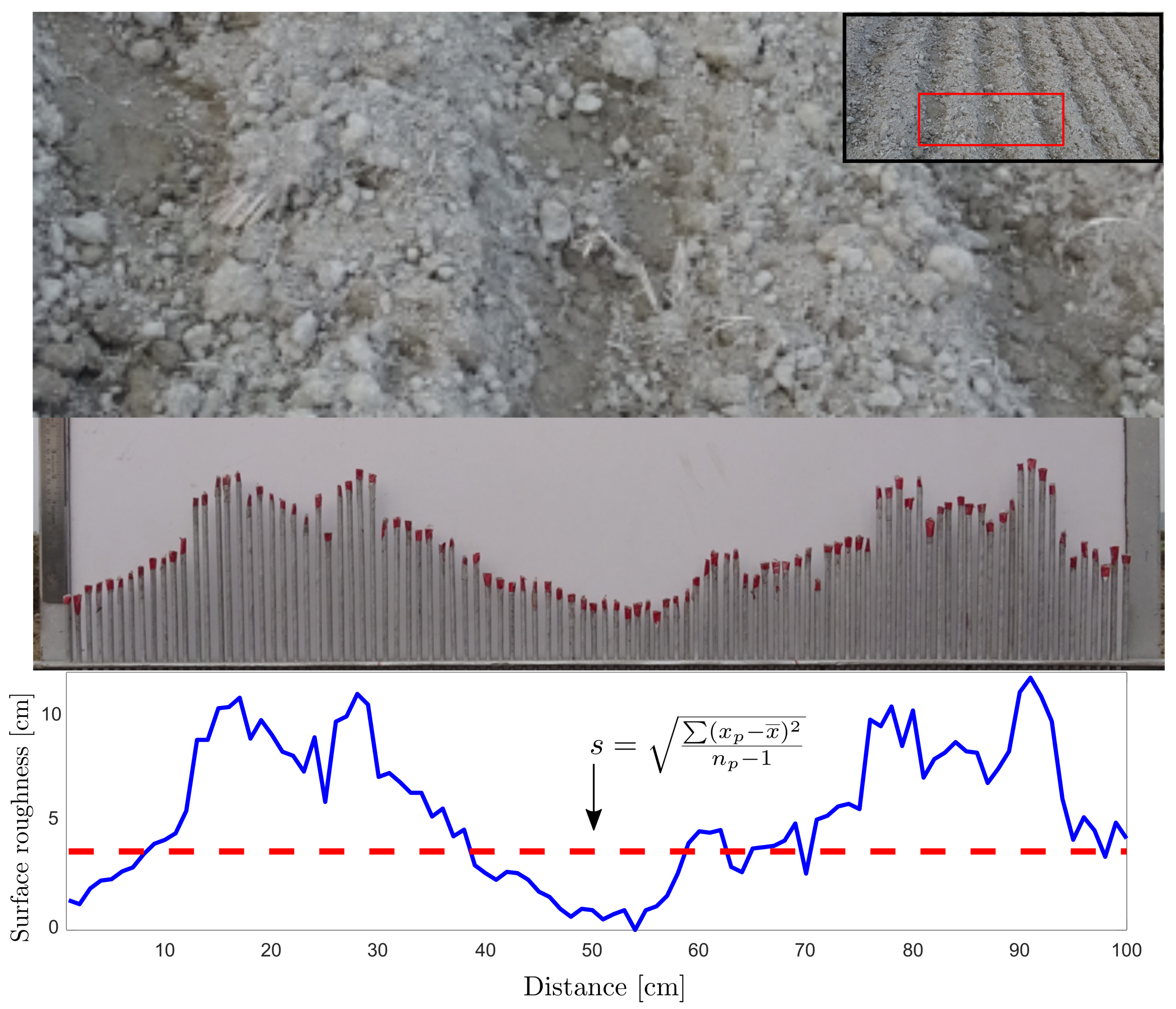
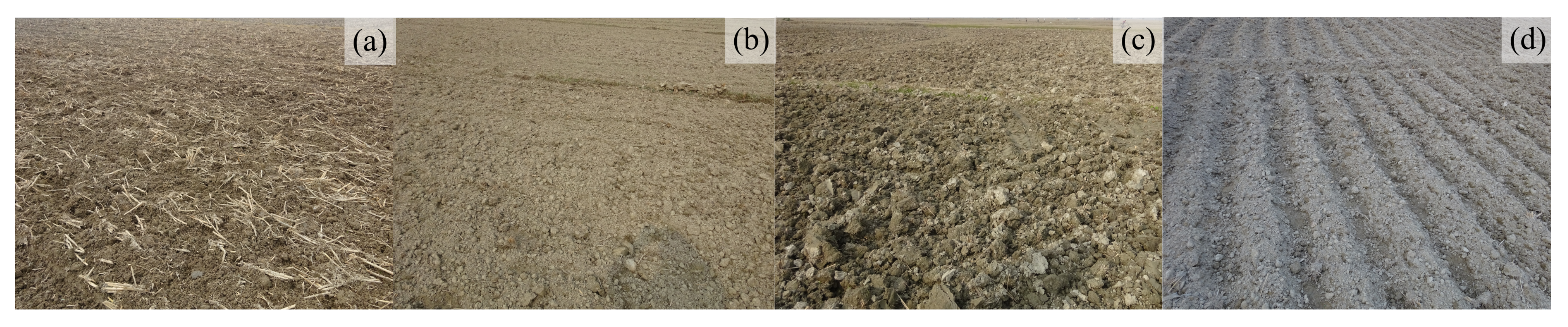
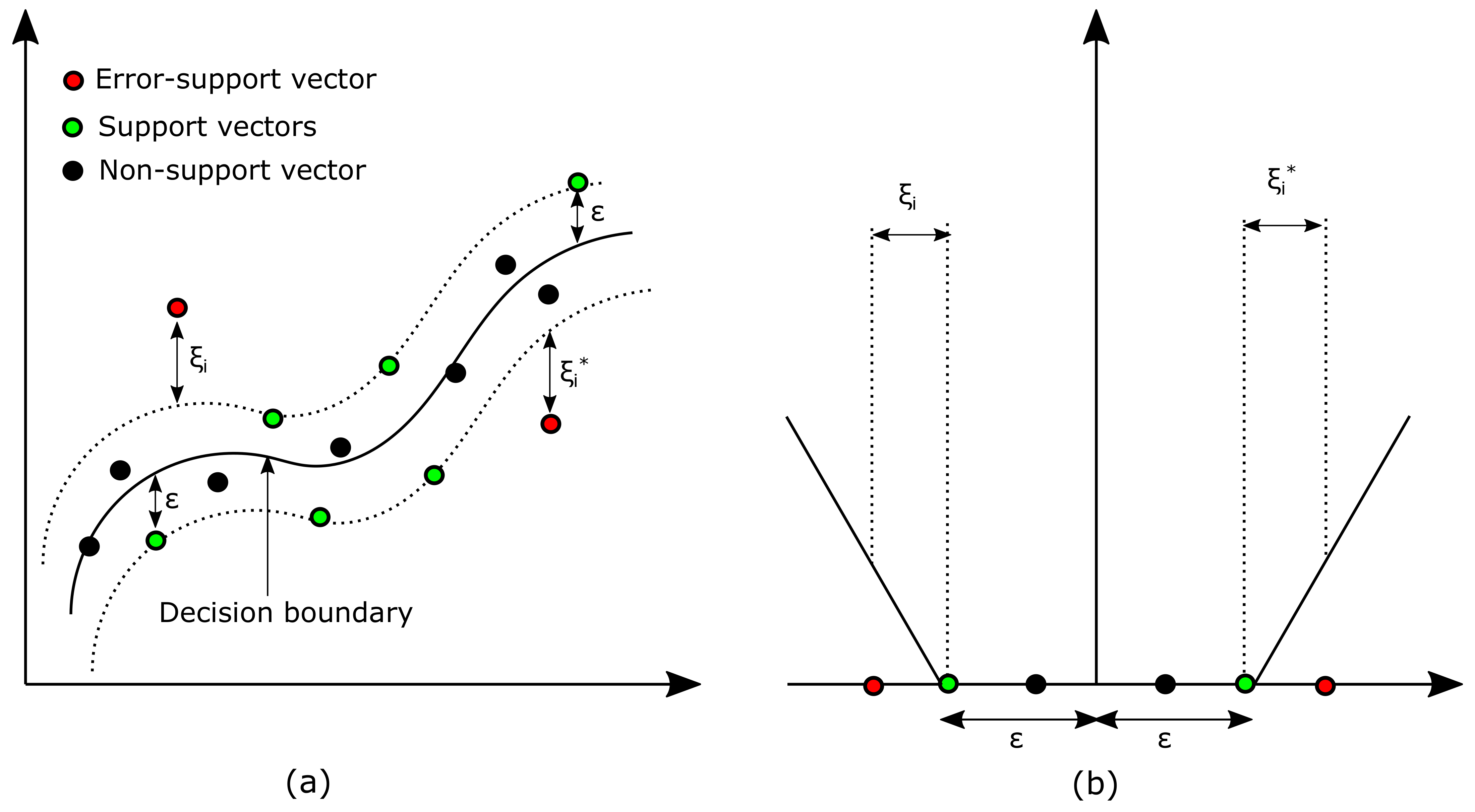
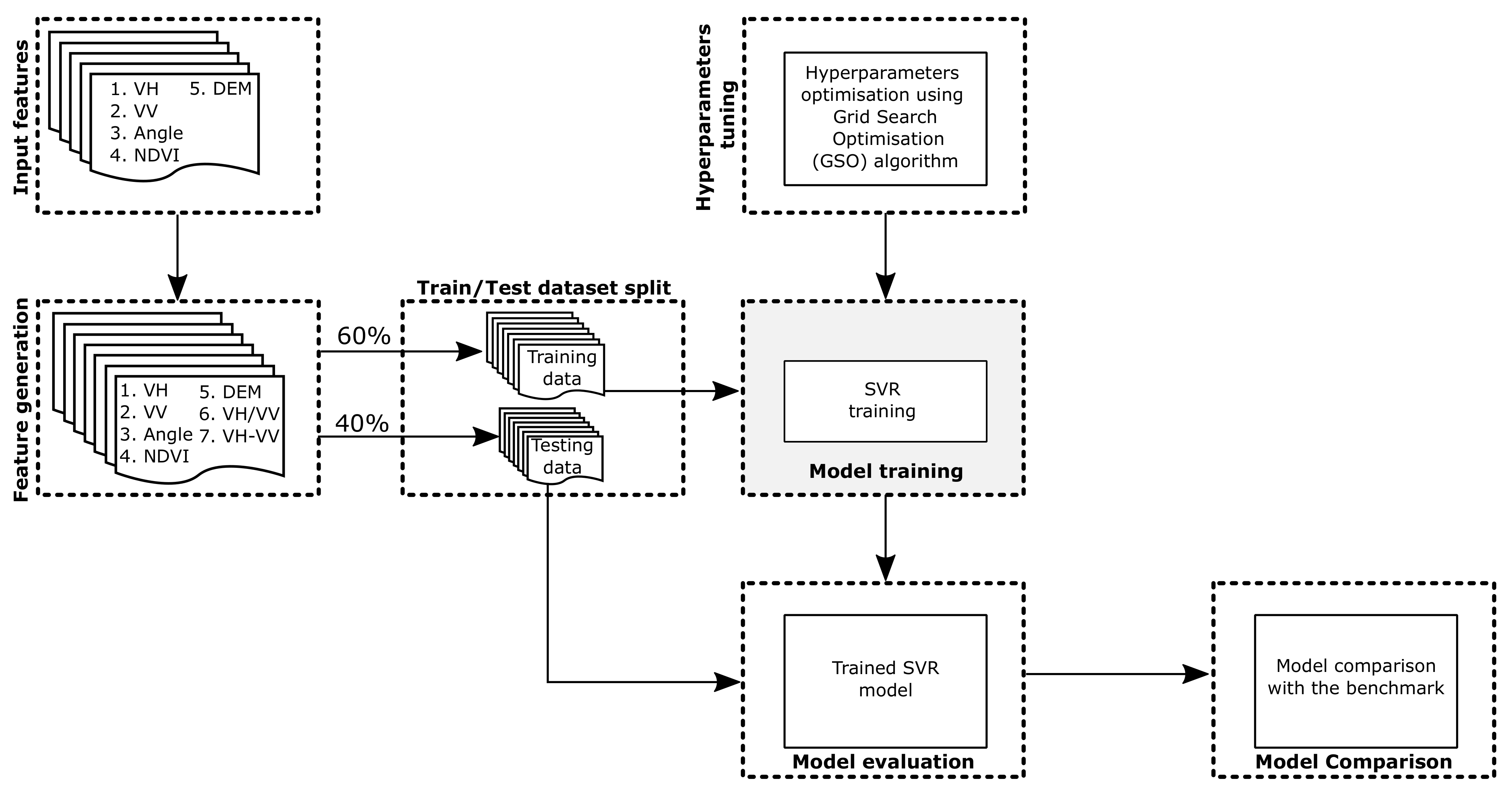
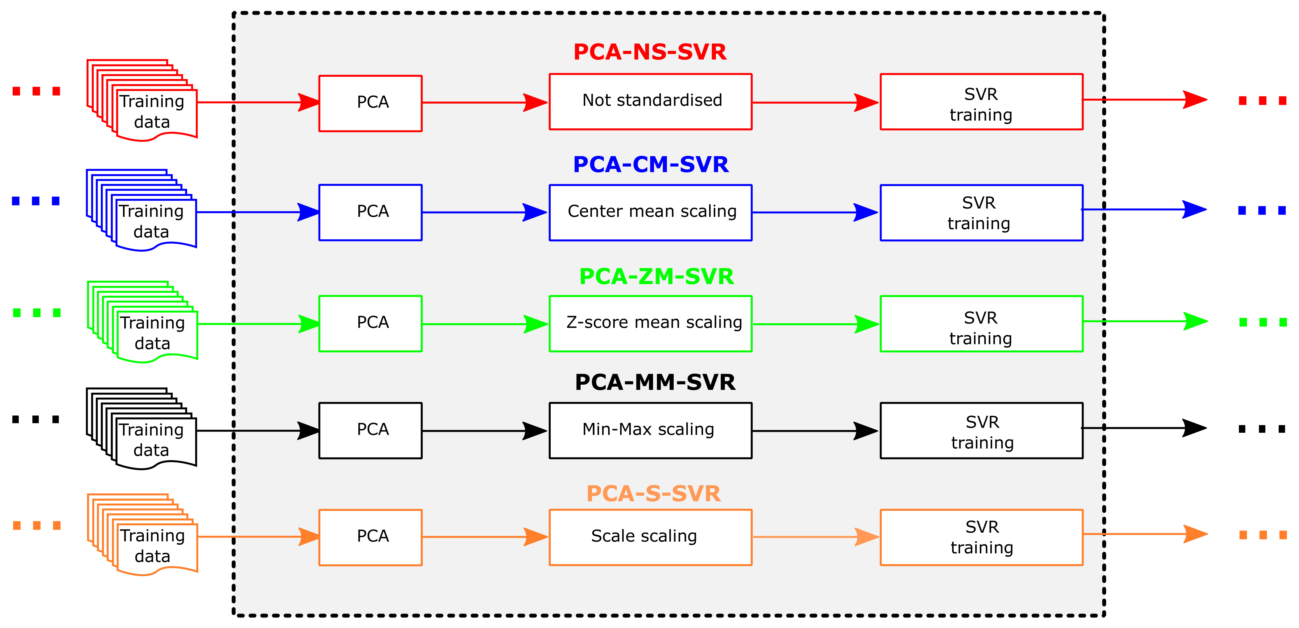
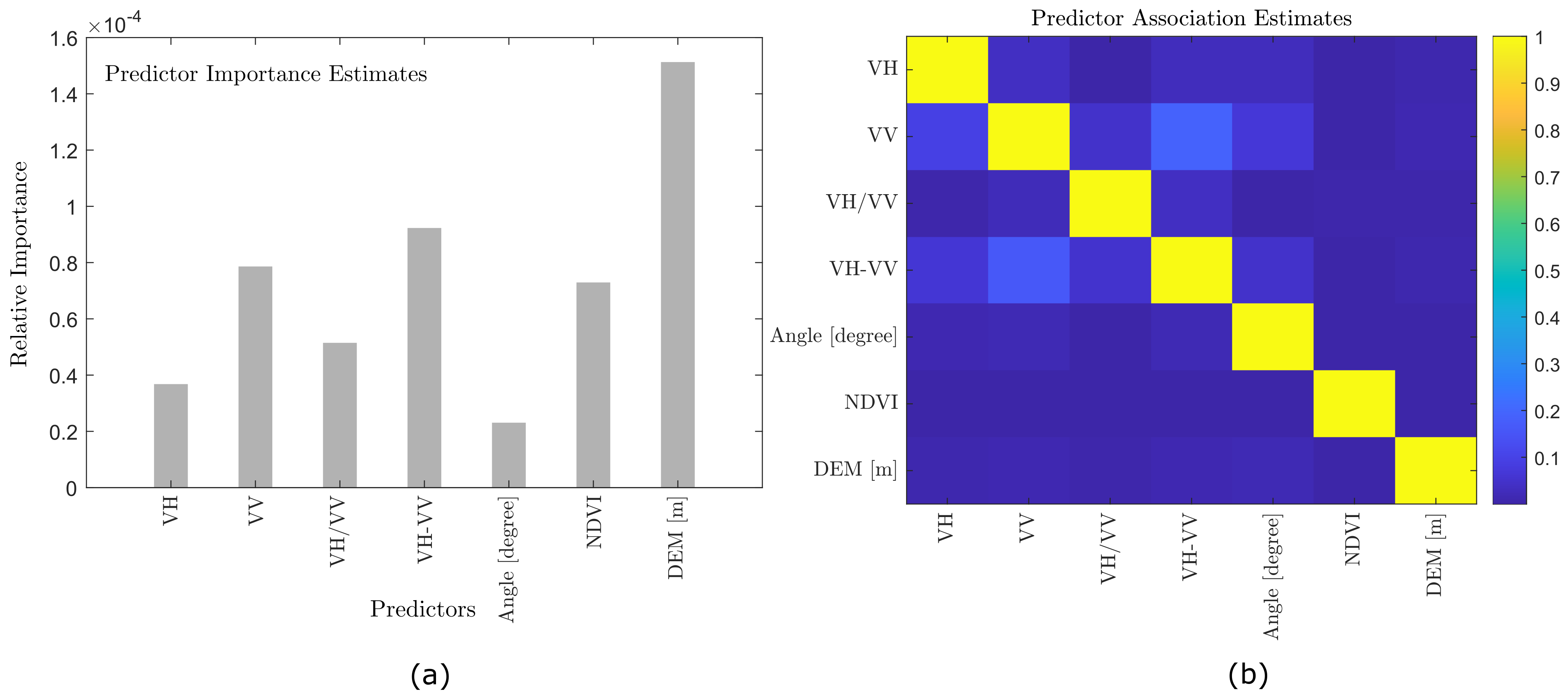
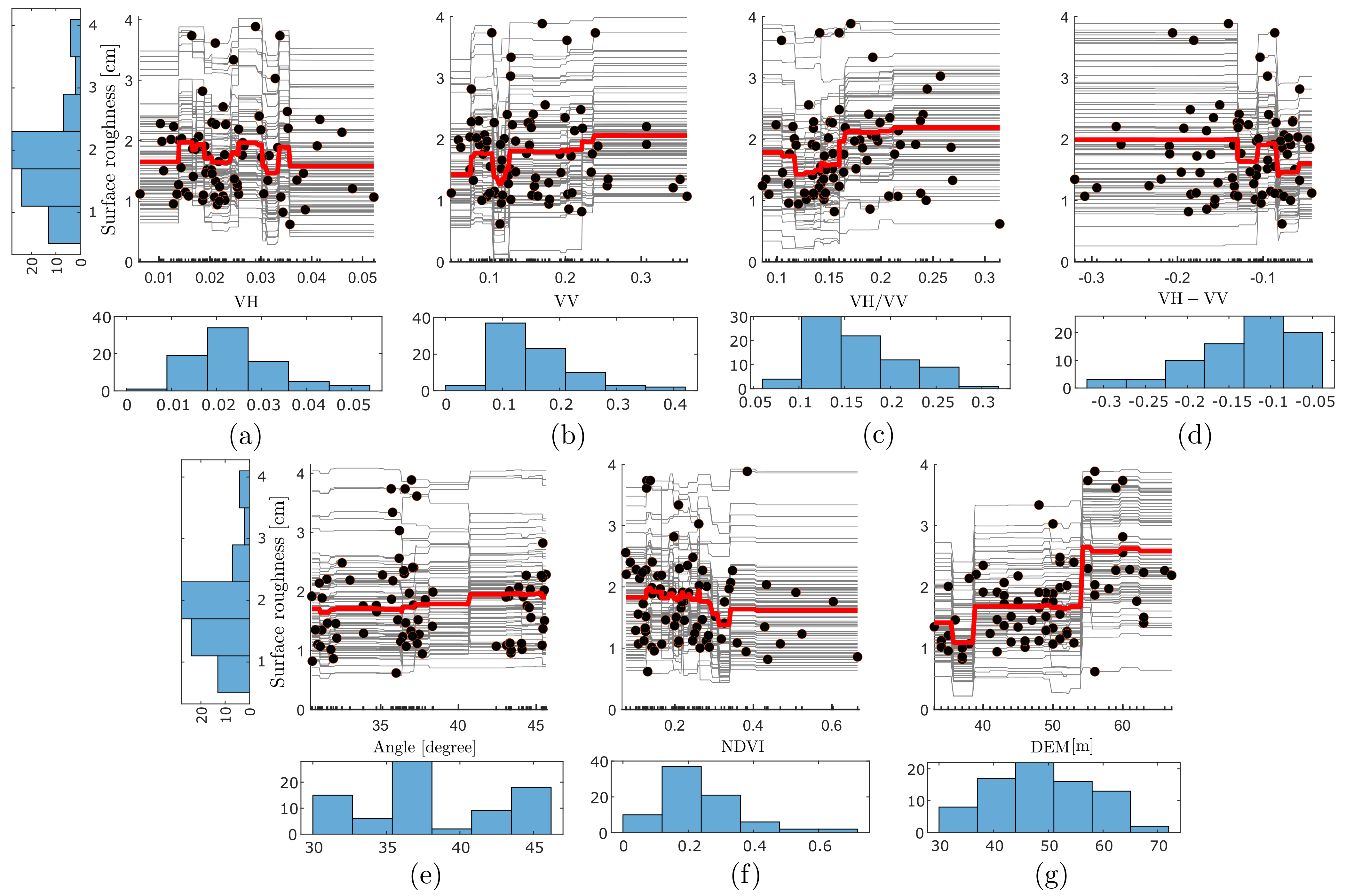
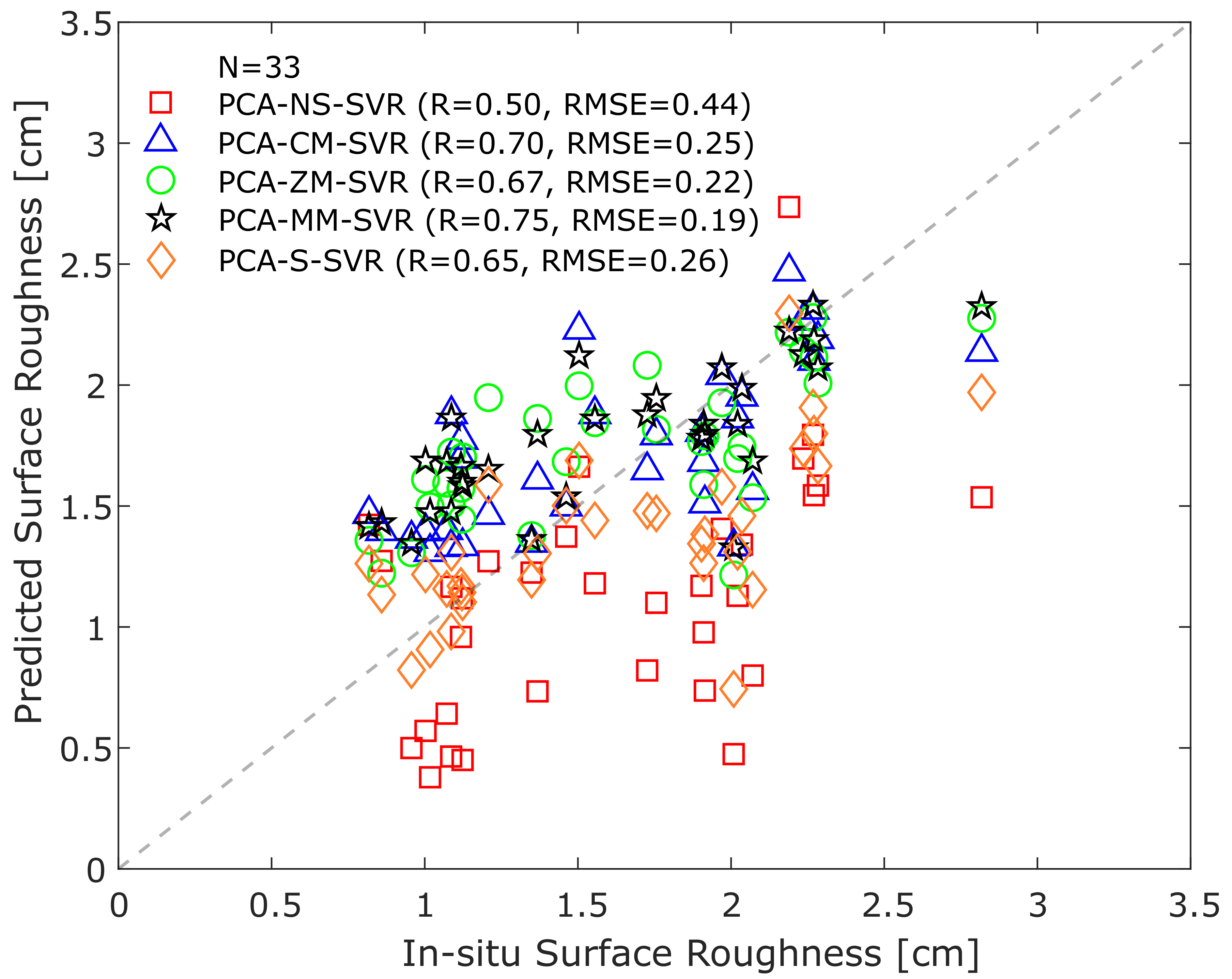
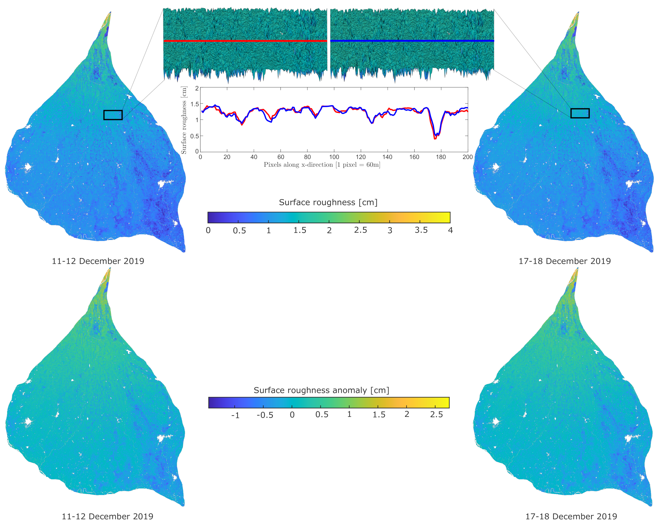

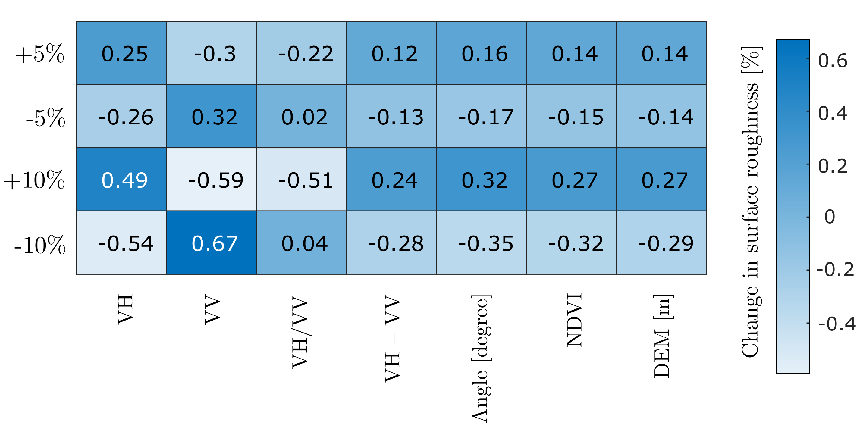
Publisher’s Note: MDPI stays neutral with regard to jurisdictional claims in published maps and institutional affiliations. |
© 2021 by the authors. Licensee MDPI, Basel, Switzerland. This article is an open access article distributed under the terms and conditions of the Creative Commons Attribution (CC BY) license (https://creativecommons.org/licenses/by/4.0/).