Abstract
Exposure to fine particulate matter (PM) air pollution has been shown in numerous studies to be associated with detrimental health effects. However, the ability to conduct epidemiological assessments can be limited due to challenges in generating reliable PM estimates, particularly in parts of the world such as the Middle East where measurements are scarce and extreme meteorological events such as sandstorms are frequent. In order to supplement exposure modeling efforts under such conditions, satellite-retrieved aerosol optical depth (AOD) has proven to be useful due to its global coverage. By using AODs from the Multiangle Implementation of Atmospheric Correction (MAIAC) of the MODerate Resolution Imaging Spectroradiometer (MODIS) and the Multiangle Imaging Spectroradiometer (MISR) combined with meteorological and assimilated aerosol information from the Modern-Era Retrospective analysis for Research and Applications, Version 2 (MERRA-2), we constructed machine learning models to predict PM in the area surrounding the Persian Gulf, including Kuwait, Bahrain, and the United Arab Emirates (U.A.E). Our models showed regional differences in predictive performance, with better results in the U.A.E. (median test = 0.66) than Kuwait (median test = 0.51). Variable importance also differed by region, where satellite-retrieved AOD variables were more important for predicting PM in Kuwait than in the U.A.E. Divergent trends in the temporal and spatial autocorrelations of PM and AOD in the two regions offered possible explanations for differences in predictive performance and variable importance. In a test of model transferability, we found that models trained in one region and applied to another did not predict PM well, even if the transferred model had better performance. Overall the results of our study suggest that models developed over large geographic areas could generate PM estimates with greater uncertainty than could be obtained by taking a regional modeling approach. Furthermore, development of methods to better incorporate spatial and temporal autocorrelations in machine learning models warrants further examination.
1. Introduction
Spatially and temporally resolved estimates of particulate matter with aerodynamic diameter less than 2.5 m (PM) are of significant importance for studying the health effects associated with exposure to air pollution. Various statistical and machine learning methods have been developed for this task and have been facilitated by increases in both the quantity and types of spatio-temporal data. For instance, aerosols observed from polar-orbiting satellites, retrieved as aerosol optical depth (AOD), have become attractive for PM estimation due to their vast coverage, both spatial and temporal. Many studies have found great success in leveraging AOD to predict PM globally [1,2,3,4,5,6]. The resolution of AOD data has improved significantly in the past decade for MODerate resolution Imaging Spectroradiometer (MODIS) and Multiangle Imaging SpectroRadiometer (MISR) instruments, which originally provided AOD retrievals at 10 km and 17.6 km, respectively. Advanced processing algorithms have downscaled these retrievals to much higher resolutions (1 km and 4.4 km, respectively) with improved accuracy in validation tests [7,8].
While the spatio-temporal coverage of satellite-observed AOD has made it a key predictor in models developed to estimate PM, the majority of studies have focused on data-rich regions of the world such as the United States and China, which have large and established air quality monitoring networks to train and validate models [5,6,9,10]. In other locations such as the Middle East where ground PM monitoring is sparse or nonexistent, modeling efforts have been limited.
The air quality in Middle Eastern cities is poor, with contributing sources ranging from industry and construction to transportation [11]. Compounding these anthropogenic sources, extreme meteorological events such as dust storms further contribute to high particulate matter concentrations and make it challenging to estimate PM accurately. A recent study in Kuwait found dust events occurring in more than one third (37%) of the days observed from October 2017 through October 2019 [12], and most particle samplers are likely inadequate to collect samples during dust storms when concentrations exceed 200–400 µg/m [13]. The same study also found dust storms and road dust to be the second largest contributor (20%) to PM in Kuwait City.
While it may be desirable to apply models trained in data-rich regions to make predictions where there is little validation data, they are not guaranteed to perform well, and the estimates are likely to possess large uncertainties. Most studies estimating PM typically report an overall summary performance metric such as cross-validation , yet these statistics may be deceiving because models are unlikely to predict with the same accuracy at all locations and at all times within a given study domain. Spatial and temporal variability in predictive performance has been shown through leave-one-out (LOO) cross-validation (CV), either by leaving out one site or region or by leaving out one year in each training-validating iteration [5,14,15,16,17,18,19].
For example, differences in predictive performance have appeared in large-scale studies including Engel-Cox et al. (2004), who found that MODIS AOD showed poorer correlation with PM in the Western U.S. compared to the Eastern and Midwest U.S. [20]. In cross-validated models based on U.S. Census Bureau geographic subdivisions, Di et al. (2019) found that the western region had the poorest prediction with the mountain subdivision having the lowest CV , and the pacific subdivision having the highest CV RMSE (root mean squared error). The Midwest and southern subdivisions west of the Mississippi River also predicted worse than all subdivisions east of the river [5].
Model adjustments can be made to account for differences in predictive performance. In a global study, Shaddick et al. (2018) accounted for spatial variability in their AOD-PM models by adding random effect terms for country, region, and super-region [4]. In another global study, Hammer et al. (2020) identified divergent temporal trends in PM across regions that affected model performance, which was addressed through statistical fusion [21]. Modeling over the contiguous U.S., Di et al. (2019) included a spatially lagged term for PM to account for spatial autocorrelation [5].
Although Engel-Cox et al. (2004) and Di et al. (2019) cited sparse data (both fewer PM monitors and lower AOD retrieval success rate) and challenging terrain as reasons for heterogeneity in model performance, few studies have investigated other possible mechanisms. We suggest that trends in spatial and temporal autocorrelation for PM, AOD, and possibly meteorology could impact the strength of the correlation between PM and model predictors. Several studies have examined the spatial and temporal autocorrelation (or coherence) of PM and AOD, yet its potential impact on models predicting PM has remained underexplored.
Sullivan and Pryor (2014) found that PM temporal variability had an impact on both natural and anthropogenic cycles and indicated that there was a link between PM concentrations and meteorological conditions. They also found that, at a subdaily scale, spatial variability was 2–3 times greater than temporal variability [22]. In another study of MODIS AOD over eastern North America, Sullivan et al. (2015) found that spatial coherence r for AOD dropped below 0.3 at ∼750 km on average, and that the range of the semivariogram for the summer was almost twice that of the winter (∼2200 km vs. ∼1300 km, respectively) [23].
Toth et al. (2019) studied decay in spatial correlation for PM in the contiguous U.S. (CONUS) and found the e-folding length in correlation (distance or time for correlation to reduce below 1, about 0.37) to be ∼600 km; regional analysis by 10 km bin averages found the e-folding length to be ∼700 km in the eastern CONUS and ∼300 km in the western CONUS [24]. In their temporal autocorrelation analysis in the Southeastern U.S., Kaku et al. (2018) found that the e-folding time was 3 days for ground-monitored PM and only 1 day for ground-monitored AERONET AOD. The authors noted that strong single-day spikes in AOD—and hence day-to-day variability—were far more prevalent in AOD than in PM [25].
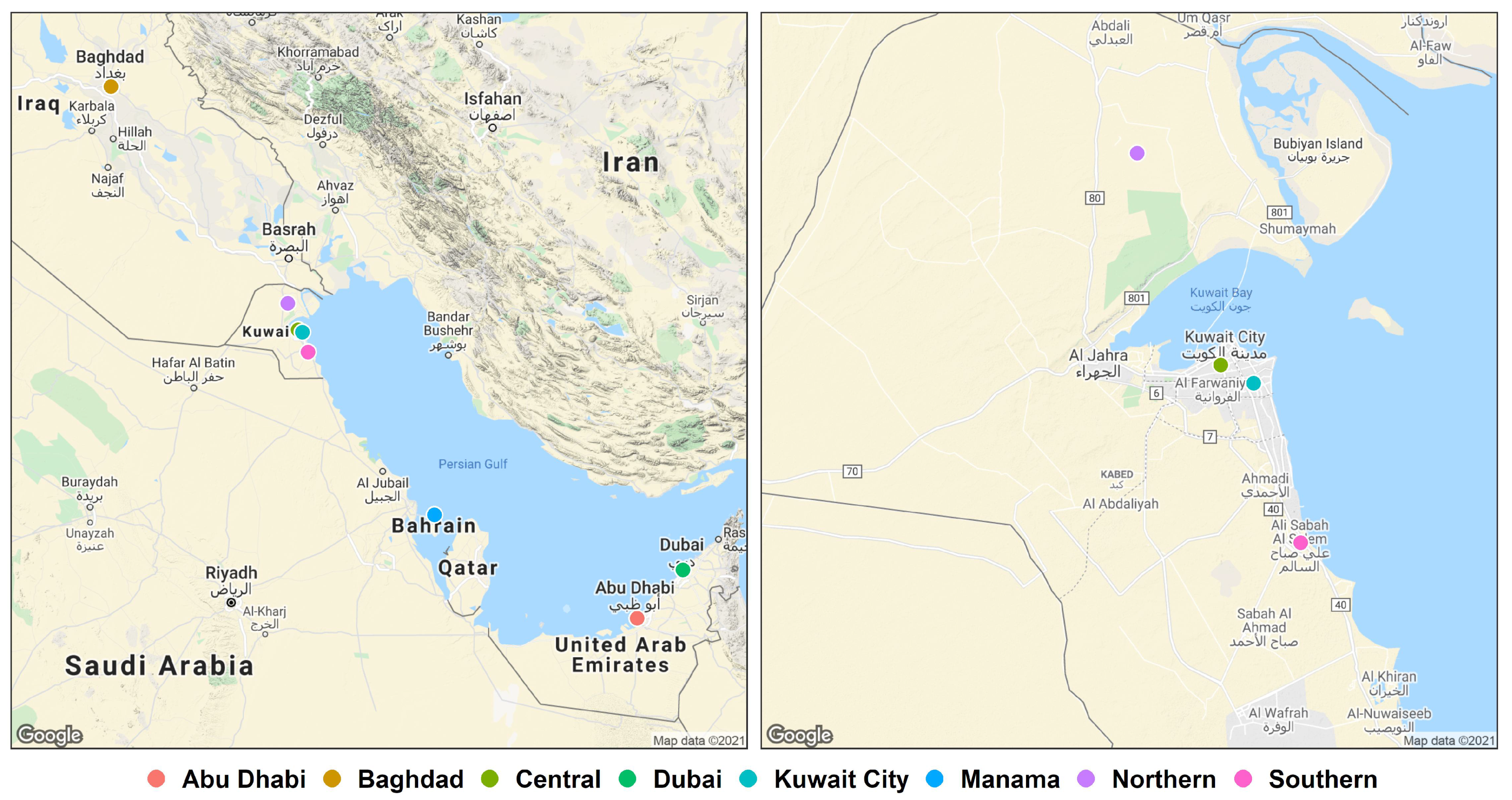
Using the Middle East as our study region (Figure 1), we developed AOD-PM models, evaluated their overall and regional predictive performance, examined the spatial heterogeneity in model performance, identified the most important predictors, and explored the impact of spatial and temporal autocorrelation on relationship between PM AOD, and other predictors.
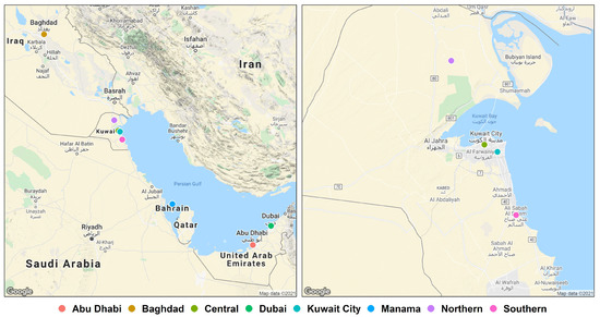
Figure 1.
Map of the study region with all PM monitors (left) and only those in Kuwait (right).
2. Materials and Methods
2.1. Particulate Matter Data
The PM data used in this study were obtained from two sources. Through a collaborative project between researchers from Kuwait University and the Harvard School of Public Health, PM data were collected in years 2004–2005 and 2017–2019 at three locations in Kuwait: a “central” site at Kuwait University, a “northern” site in Um-Al-Aish—approximately 55 km north of Kuwait City in the Al Jahra Governorate—and a “southern” site in Um-Al-Haiman—approximately 45 km south of Kuwait City in Ali Sabah Al Salem. The central and southern sites were in urban areas, and the northern site is in a desert area. Due to high concentrations of PM and extreme temperatures in the region, Harvard high-capacity impactors were used to sample PM [26,27]. We refer to these data as the HHI PM dataset.
The second source of data was OpenAQ, an open-source platform that provides real-time and historical air quality data. OpenAQ aggregates government-measured and research-grade data from different government entities and international organizations [28]. For this study, we acquired PM data from measurements taken at United States embassies and consulates from five cities in four countries: Bahrain (Manama), Iraq (Baghdad), Kuwait (Kuwait City), and United Arab Emirates (Abu Dhabi and Dubai). PM data were available as early as 2016 (Manama), and we included data collected up to mid-June, 2020. We refer to these data as the OpenAQ PM dataset.
2.2. Aerosol Optical Depth Data
Launched in December 1999, the polar-orbiting Terra satellite carries two instruments that observe atmospheric aerosols: the MODerate resolution Imaging Spectroradiometer (MODIS) and the Multi-angle Imaging SpectroRadiometer (MISR). The MODIS instrument uses a single sensor with a wide observation swath and provides daily aerosol observations globally. Initially available at 10 km resolution, MODIS data have been reprocessed using the Multi-Angle Implementation of Atmospheric Correction (MAIAC) and are currently available at 1 km resolution [8]. We refer to these as MAIAC AOD data.
The MISR instrument relies on nine camera angles and four spectral bands to discern aerosol particles of different sizes, shapes, and types. In addition to total column AOD, MISR provides AODs fractionated into small, medium, and large (amount of particles of each size); nonspherical (amount of nonspherical particles); and absorption (amount of light-absorbing particles). One limitation of MISR is that, due to its narrower observation swath, the instrument only overpasses any given location every 3–5 days. Originally available at 17.6 km resolution, MISR AOD data have also been improved and reprocessed, and the latest version (V23) is available at 4.4 km [7].
The MISR quality-control procedures sometimes reject observations that are deemed “low-quality”, one reason being unusually high values. However, all original AOD observations are still preserved in the “AUXILIARY” subgroup of the MISR AOD product files and are labeled “raw” (e.g., raw total AOD, raw small AOD, and raw absorption AOD). The “raw” version of each AOD variable contains both the “high-quality” and “low-quality” observations; therefore, it typically provides a slightly larger sample size. As extreme weather conditions such as sandstorms are typical in our study region, we considered the raw AOD variables for modeling PM. Although we fitted predictive models using both “high-quality” and “raw” AOD data, we will only report results of models with “raw” AOD variables as they consistently predicted better than those with “high-quality” AOD variables. For the remainder of this paper, we refer to the “raw” MISR AOD variables simply as MISR AOD, except for the AERONET AOD validation portion where we report both and will be specific in that context.
2.3. Meteorology Data
Following previous modeling approaches [29], we incorporated meteorological data to improve PM predictions. For this study, we relied on reanalysis data from the European Centre for Medium-Range Weather Forecasts (ECMWF), version 5 (ERA5). ERA5 provides a wide range of meteorological data at hourly temporal and approximately 31 km horizontal resolution [30]. We extracted ERA5 meteorological variables including wind speed, wind direction, temperature, evaporation, surface pressure, cloud cover, precipitation, relative humidity, boundary layer height (BLH), and downward shortwave (UV) radiation, which we identified to be a key predictor variable in previous studies [29,31,32].
2.4. Assimilated Aerosol Data
We also incorporated assimilated aerosol optical depth data from the Modern Era Retrospective Analysis for Research and Applications, version 2 (MERRA-2), which is the latest atmospheric reanalysis of the modern satellite era produced by NASA’s Global Modeling and Assimilation Office (GMAO) [33,34]. Although MERRA-2 data are provided at relatively low resolution (∼50 km), their source-specific AODs have proven to be useful for estimating PM in other studies [5,35,36]. While there have been some efforts to downscale MERRA-2 to a finer spatial resolution [35], in this study we used MERRA-2 AOD variables (dust, black carbon (BC), organic carbon (OC), and sulfate (SO)) at their native resolution.
2.5. Statistical Methods
We validated MAIAC and MISR AOD against AOD from the Aerosol Robotic Network (AERONET). AERONET is an instrument network of ground-based sun photometers that derive AOD at a number of visible and near-infrared wavelengths from direct sun observations and has served as the primary standard for validating satellite aerosol products [37]. We matched MAIAC and MISR AOD to the Kuwait University AERONET when it was active between 2006 and 2010 by identifying the nearest MAIAC AOD observation within 1 km and the nearest MISR AOD observation within 4.4 km of the AERONET site. As AERONET only measures AOD at 500 nm and 675 nm, we interpolated it to 550 nm in order to match total column AOD from both MAIAC and MISR [19]. We averaged AERONET AOD to the nearest hour and filtered measurements to match the Terra satellite overpass time (between 10:00 and 12:00 local time). Validation statistics including linear correlation (r), RMSE, and bias between AERONET AOD, MAIAC and MISR AOD were calculated.
We used a selection of five different machine learning models [29,38] in a regression framework (LASSO regression, ridge regression, gradient boosting machines (GBM), random forests (RF), and support vector machines (SVM)) [39]. In previous studies, non-linear methods (GBM, RF, and SVM) demonstrated stronger predictive performance compared to linear learners (LASSO and ridge), due to the non-linear relationship between PM and satellite-observed AODs [29,38,40]. We considered linear methods to assess whether the pattern of non-linearity held in this region with more extreme climate conditions.
We fitted separate predictive models for MAIAC AOD and for the six fractionated MISR AODs (total, small, medium, large, nonspherical, and absorption). In both cases, we included ERA5 meteorological variables, MERRA-2 assimilated AODs, spatial coordinates (the latitude and longitude of MAIAC or MISR pixels), and time (Julian date and month). For each machine learning method, the model was trained on 70% of the data, and we selected the best fitting hyperparameters based on as the performance metric by using 10-fold cross validation. The models with the best performing hyperparameters were then assessed on the remaining 30% test sample of data and also via . Due to the small sample size of our data, particularly for the MISR-AOD dataset, the trained models could be very sensitive to the observations in the training set. Therefore, we repeated this training-testing process in 25 iterations, each time drawing a different 70–30 split in the data, in order to assess the stability and robustness of each model. The models with the best median prediction test were chosen as the final models.
Leave-one-out (LOO) cross-validation, typically reserving a single site or region, or a time unit (e.g., year) for out-of-sample validation, is a common approach for assessing model generalizability—a key component of predictive modeling using machine learning techniques [5,41]. Given the small number of PM monitoring sites (eight sites) in our sample, the overall small sample size, and the unbalanced sample sizes across regions, this approach was less useful in our study, and so it was not conducted (Kuwait and the U.A.E., respectively, made up 50% and 25% of the MISR-AOD data and 56% and 19% of the MAIAC-AOD data).
In addition to developing a model using data from all sites, we divided the study region into two subregions: Kuwait (four sites) and the U.A.E. (two sites). We excluded Manama and Baghdad from this portion of the analysis as they each had only one PM monitoring site and, thus, provided little spatial variability. For the iterated training-testing process described above, we calculated both the overall test and the regional test using the data that included all sites. Furthermore, we fitted separate models using only data from each subregion; this was also performed once with MAIAC AOD and once with fractionated MISR AODs. These regional models allowed us to assess the transferability of the models—i.e., predicting PM over an area using a model trained in a completely different location. Specifically, we used the Kuwait-trained models to predict PM in the U.A.E. and used the U.A.E.-trained models to predict PM in Kuwait and assessed their respective prediction .
For the best performing machine learning method, we estimated variable importance to understand the relative importance of satellite-observed aerosol variables among the models considered (MAIAC AOD vs. MISR AODs and overall vs. regional). Variable importance was calculated by using permutation accuracy importance, which is based on the increase in mean squared error (MSE) when a variable is excluded, as it is more robust to bias than the typical Gini impurity importance, which is based on node purity [42]. In order to verify variable importance for AOD variables in these models, we fitted the same models without satellite AOD predictors and assessed their predictive performance ().
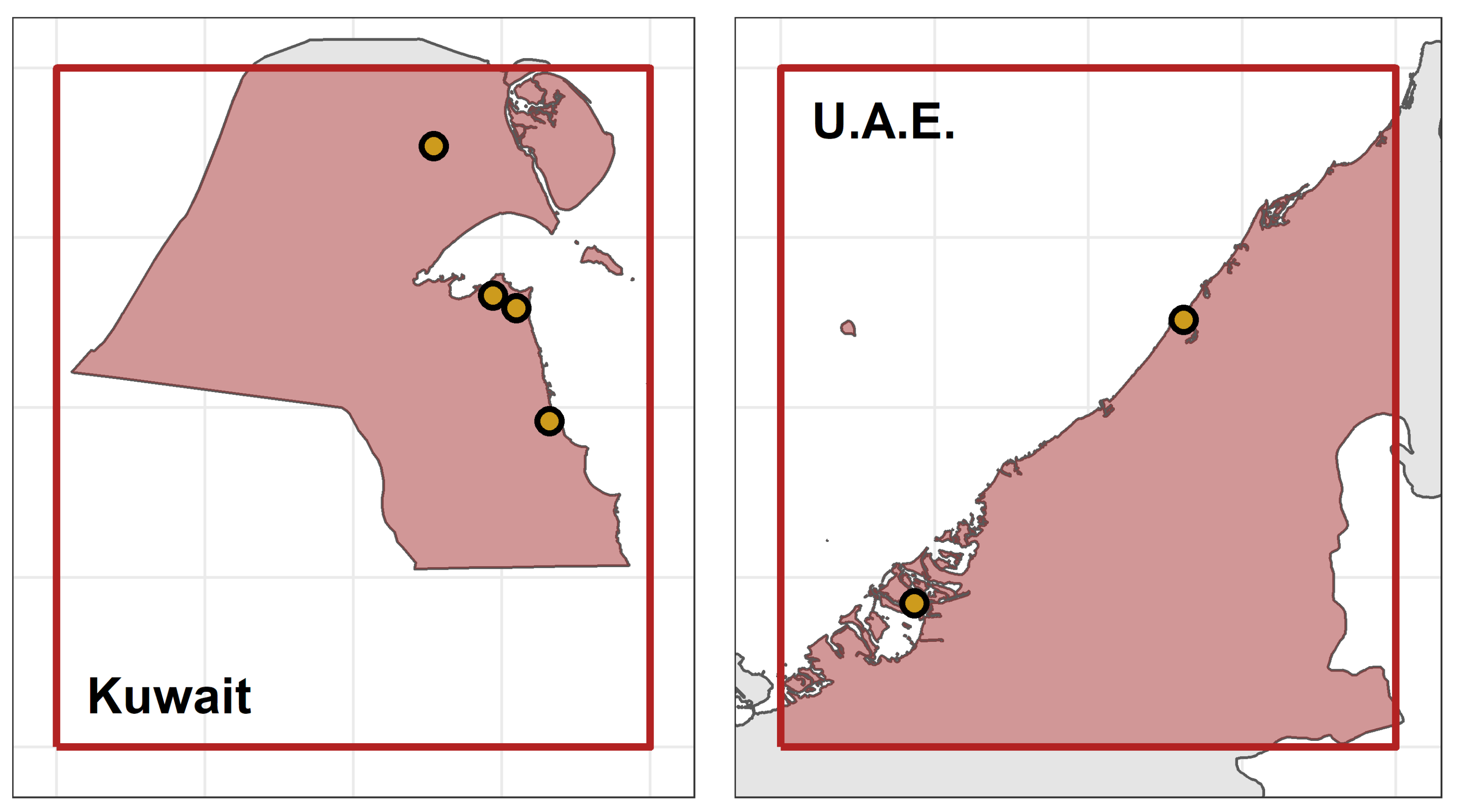
Possible explanations for differences in performance and variable importance between subregions were explored by estimating temporal and spatial autocorrelations. The temporal autocorrelation function (ACF) was assessed for PM, AOD, MERRA-2 variables, and ERA5 meteorological variables at the Kuwait and U.A.E. PM monitoring locations. Due to the temporal gaps in MISR AODs (i.e., MISR being able to retrieve every 3–5 days for a given location), high-resolution temporal ACFs for satellite observed aerosols were only assessed by using MAIAC AODs. The abundance of MAIAC data also allowed for autocorrelation to be assessed more extensively. We collected MAIAC AOD in 2017–2019 for every pixel retrieved over land within a 2 degree by 2 degree area that covered the PM monitors in each country (Figure 2).
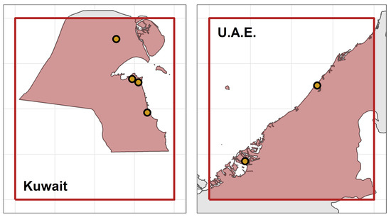
Figure 2.
Areas within each country where temporal and spatial autocorrelations for MAIAC AOD were evaluated (shaded pink) and the PM monitors (yellow circles) in each country.
Instead of examining only coincident MAIAC pixels at each site, we estimated ACF for AOD at every MAIAC pixel within 50 km of each site, and then we used these ACFs to calculate the median ACF for each site. In order to assess spatial autocorrelation, we estimated the daily empirical semivariograms [43] in 1 km bins up to 50 km for each region, and we calculated the median semivariogram over the 3 year period. Due to the lower resolution of ERA5 and MERRA-2 data (31 and 50 km, respectively), assessment of the spatial autocorrelation was only conducted for MAIAC AOD.
3. Results
3.1. AOD Validation
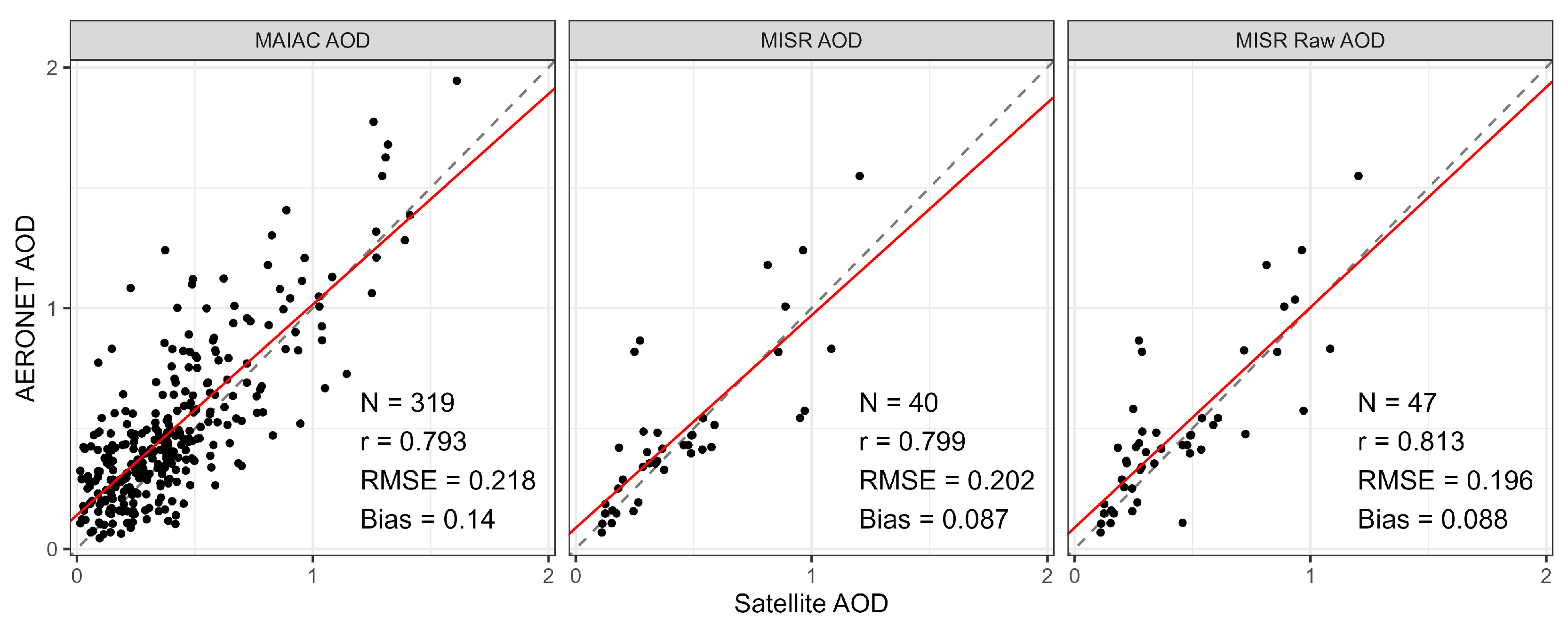
From 2006 through 2010, the Kuwait University AERONET monitor measured AOD on 421 days. Of these observations we were able to match MAIAC AOD on 319 days, MISR AOD on 40 days, and MISR “raw” AOD on 47 days. Overall, all three satellite-observed AOD samples showed strong correlations with ground-observed AERONET AOD (–0.81, Figure 3). Although there were fewer MISR AOD samples, they showed slightly better correlation with AERONET AOD ( for AOD and for “raw” AOD) compared to MAIAC AOD (). The larger r for MISR “raw” AOD over MISR AOD was likely due to a larger sample that included AOD observations that were highly correlated with AERONET AOD (Figure 3). Finally, MAIAC AOD showed a larger bias (0.140) relative to AERONET AOD compared to that of MISR AOD (0.087) and MISR “raw” AOD (0.088).
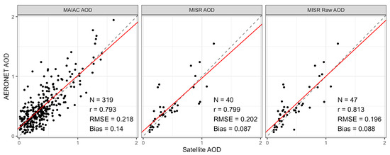
Figure 3.
Validation of AERONET AOD interpolated to 550 nm versus MAIAC AOD (left), MISR AOD (center), and MISR “raw” AOD (right) with one-to-one line (dotted) and correlation line (red).
3.2. Model Results
From February 2004 to February 2020, we were able to match PM data (three sites from HHI and five from OpenAQ in the entire study region including four countries) to 411 unique days of MISR (raw) AOD data and 1454 unique days of MAIAC AOD data for model building. The PM data included a 10 year temporal gap between 2005 and 2016: Only HHI monitors were active during 2004–2005 and were active again during 2017–2019; OpenAQ monitors in the study region began monitoring as early as 2016. Predictive performances of the full models are summarized in Table 1.

Table 1.
Median test across machine learning methods, AOD sources, and samples.
The models using data from the entire study region generally did not predict well and, at best, could only explain approximately 50% of the variability in PM in the test set. Non-linear machine learning methods performed better than linear methods, with random forest demonstrating the highest predictive performance. Non-linear models had similar test between MISR and MAIAC despite the large difference in sample size ( for MISR and for MAIAC) while the linear models performed much worse for MAIAC.
The ten most important variables in the RF models are shown in Figure 4 in descending order of importance. Variable importance was measured by percentage increase in MSE; although the absolute percentages of increase in MSE were fairly small for each variable excluded, their relative proportions are more meaningful in understanding variable importance [42]. In the MISR model, total column AOD was responsible for the largest increase in MSE when excluded, and size-fractionated AOD variables were also among the ten most important. Although total column AOD was also among the ten most important variables for the MAIAC model, its importance was relatively smaller than those of MERRA-2 dust, temperature, and boundary layer height. MISR models performed better when MERRA-2 sulfate extinction was included, while MAIAC models preferred MERRA-2 black carbon extinction.
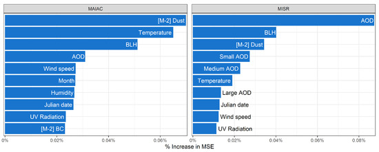
Figure 4.
The top 10 most important variables for the random forest overall models using MAIAC AOD (left) and MISR AOD (right), as measured by increase in MSE when excluded.
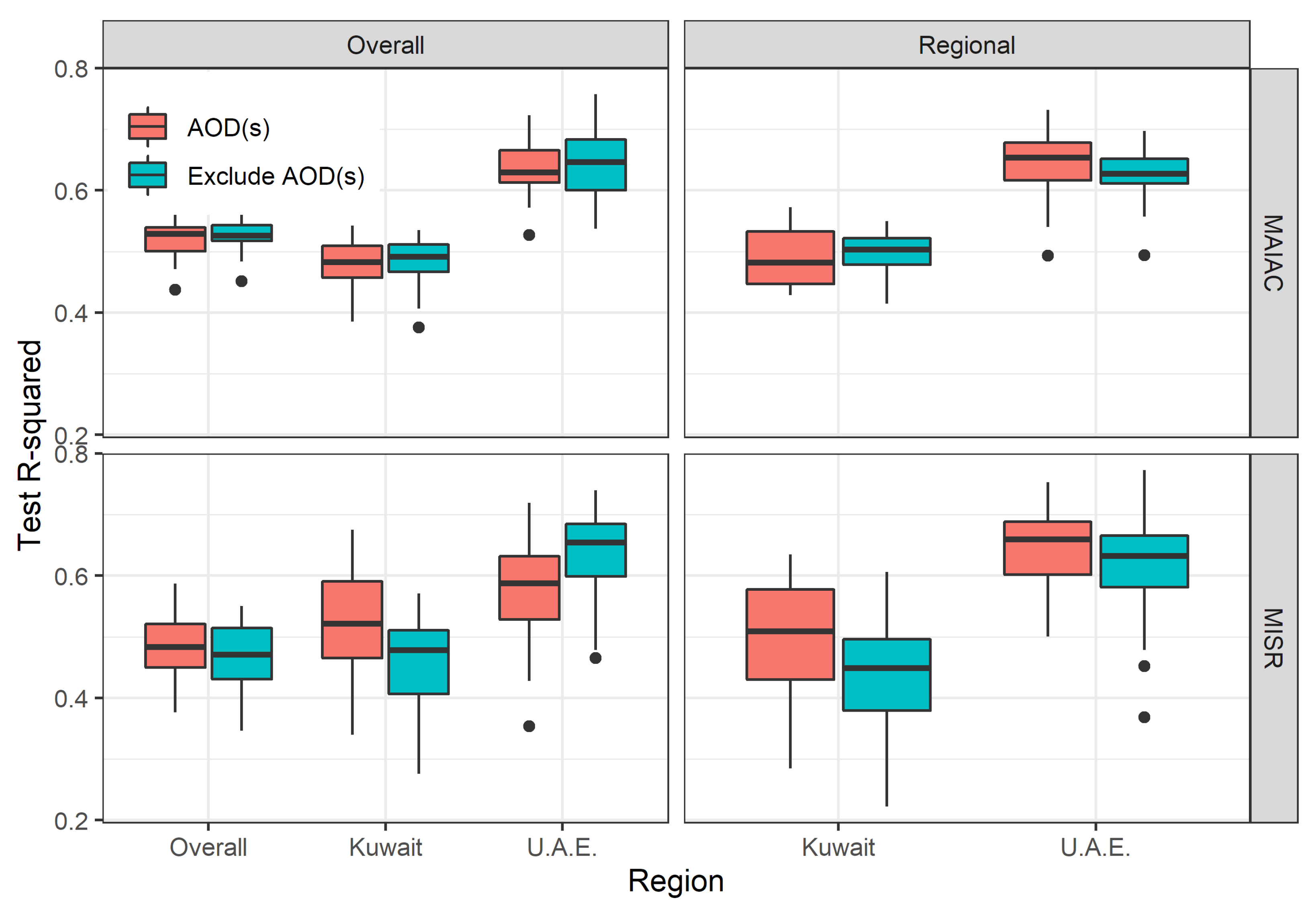
In our regional analysis, the RF model using MAIAC AOD resulted in higher prediction for the U.A.E. than for Kuwait (median test and , respectively; Table 1). Relative to the overall test , the RF model predicted slightly poorer in Kuwait and significantly better in the U.A.E. These results are fairly stable and robust to different training-testing splits (i.e., narrow boxplots, Figure 5). The RF model using fractionated MISR AODs also predicted better in the U.A.E. than in Kuwait (median test and , respectively). Relative to the overall test , the regional models predicted slightly better in Kuwait and much better in the U.A.E. (the lower overall was likely due to poorer prediction results in Baghdad and Manama, which are not shown). Wider boxplots indicated that the MISR-AOD model was more sensitive to different training-test splits, which was expected due to the smaller sample size (Figure 5).
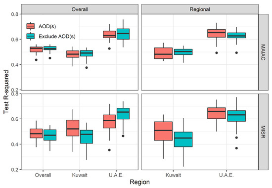
Figure 5.
Test across different settings: overall and regional models, MISR and MAIAC models, and models with and without AOD variables.
For Kuwait, the MISR model had total column AOD and MERRA-2 dust as the two most important variables in the RF models; the nonspherical AOD was among the ten most important variables along with size-fractionated AOD (Figure 6). Similar to the overall model, MAIAC AOD was not as important as MERRA-2 dust or temperature.
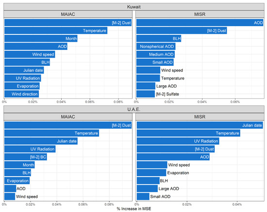
Figure 6.
The top 10 most important variables for the random forest models based on monitors in Kuwait using MAIAC AOD (top left) and MISR AOD (top right) and in the U.A.E. using MAIAC AOD (bottom left) and MISR AOD (bottom right), as measured by increase in MSE when excluded.
The regional models using only PM monitors in the U.A.E. showed better predictive performance with both MISR and MAIAC models explaining an additional 13–23% of the variation in the test set compared to the overall and Kuwait-specific models (Table 1). While MERRA-2 dust remained among the most important variables, total column AOD was less important, especially in the MAIAC model. Julian date, temperature, and UV radiation became much more important in both MISR and MAIAC models. For the MISR model, large and small AOD were still among the ten most important (Figure 6). Differences in predictive performance between the regional models were also observed in the overall models when test was estimated for each subregion (Figure 5).
In our assessment of model transferability, we used the RF model trained only on data in Kuwait to predict PM in the U.A.E. and vice versa, and found that both regional models performed much worse in predicting a different region than predicting their native region. In particular, the MAIAC-based and MISR-based Kuwait models were only able to explain 37.4% and 28.4%, respectively, of the variation in PM in the U.A.E. Similarly, the MAIAC-based and MISR-based models developed for the U.A.E. were only able to explain 12.8% and 13.2%, respectively, of the variation in PM in Kuwait (Figure A1). The poorer performance in the U.A.E. models was likely due to their underestimation of extremely high PM values in Kuwait.
3.3. Temporal and Spatial Autocorrelations
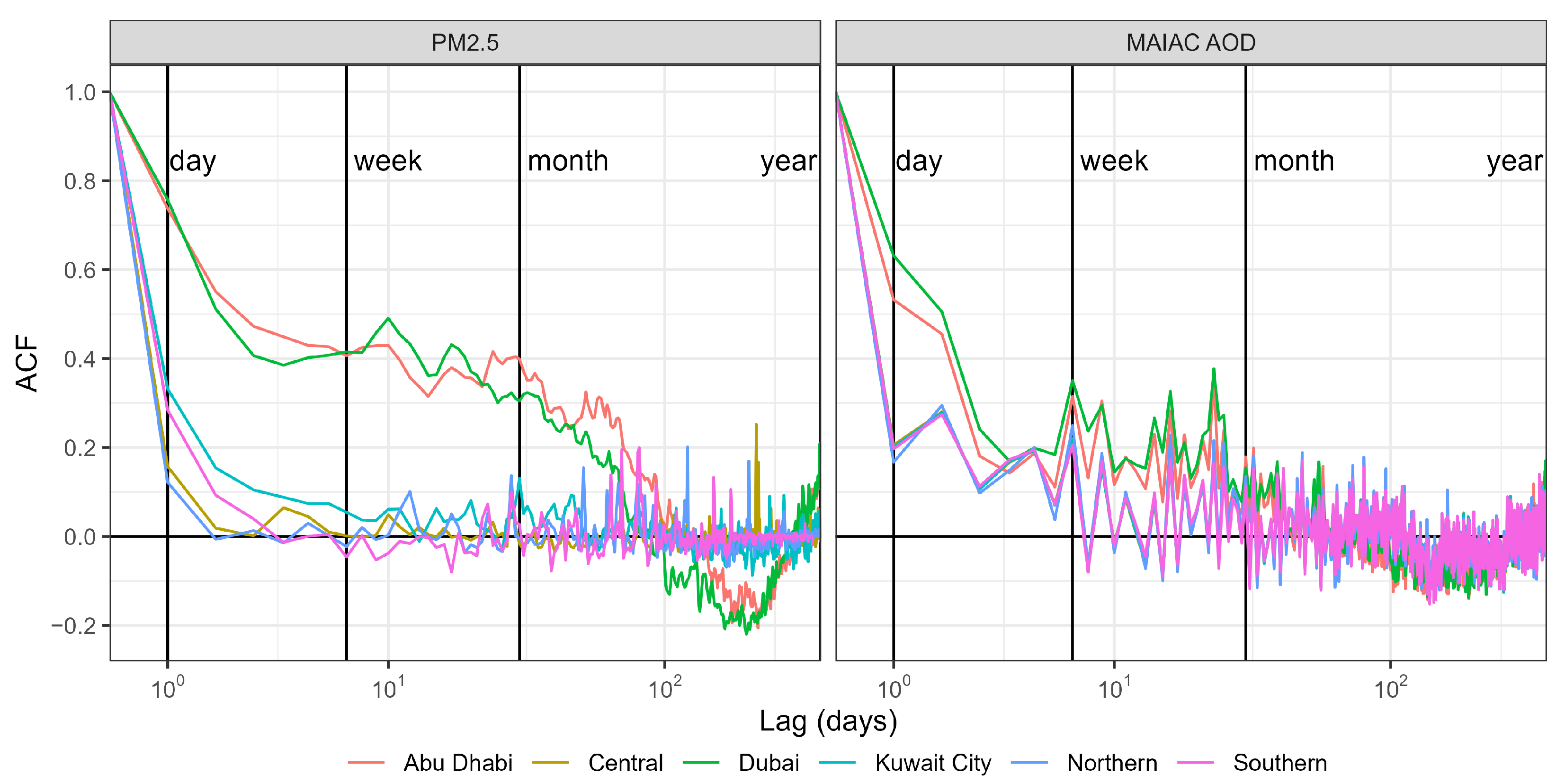
The temporal autocorrelation functions for PM and MAIAC AOD, grouped by monitor location in Kuwait and the U.A.E., are shown in Figure 7. We observed that the decay in autocorrelation was much faster in Kuwait (e-folding length—time until ACF drops below 0.37—at 1 day for all four sites) compared to both Abu Dhabi and Dubai (e-folding length at 12 and 14 days, respectively). For MAIAC AOD, the median ACFs are shown by site after aggregating the ACF for every MAIAC pixel within 50 km of each site. The autocorrelation difference between Kuwait and the U.A.E. was still observed, although it was smaller; the e-folding length at 1 day for MAIAC AOD in Kuwait and at 3 days for MAIAC AOD in the U.A.E.
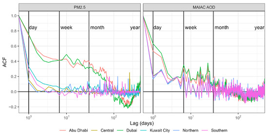
Figure 7.
Autocorrelation functions for PM (left) and median ACFs for MAIAC AOD (right) at different sites in Kuwait and the U.A.E.
Among the meteorological variables, we calculated the ACF for those with highest variable importance in the RF models: temperature, UV radiation, BLH, and wind speed (Figure A2). At all six sites in both countries, temperature and UV radiation showed very strong autocorrelations and seasonal trends. BLH and wind speed showed weaker autocorrelations (e-folding length at 3 and 2 days, respectively), with the exception of the Northern site in Kuwait where BLH had a e-folding length of almost 2 months and showed a clear seasonal trend.
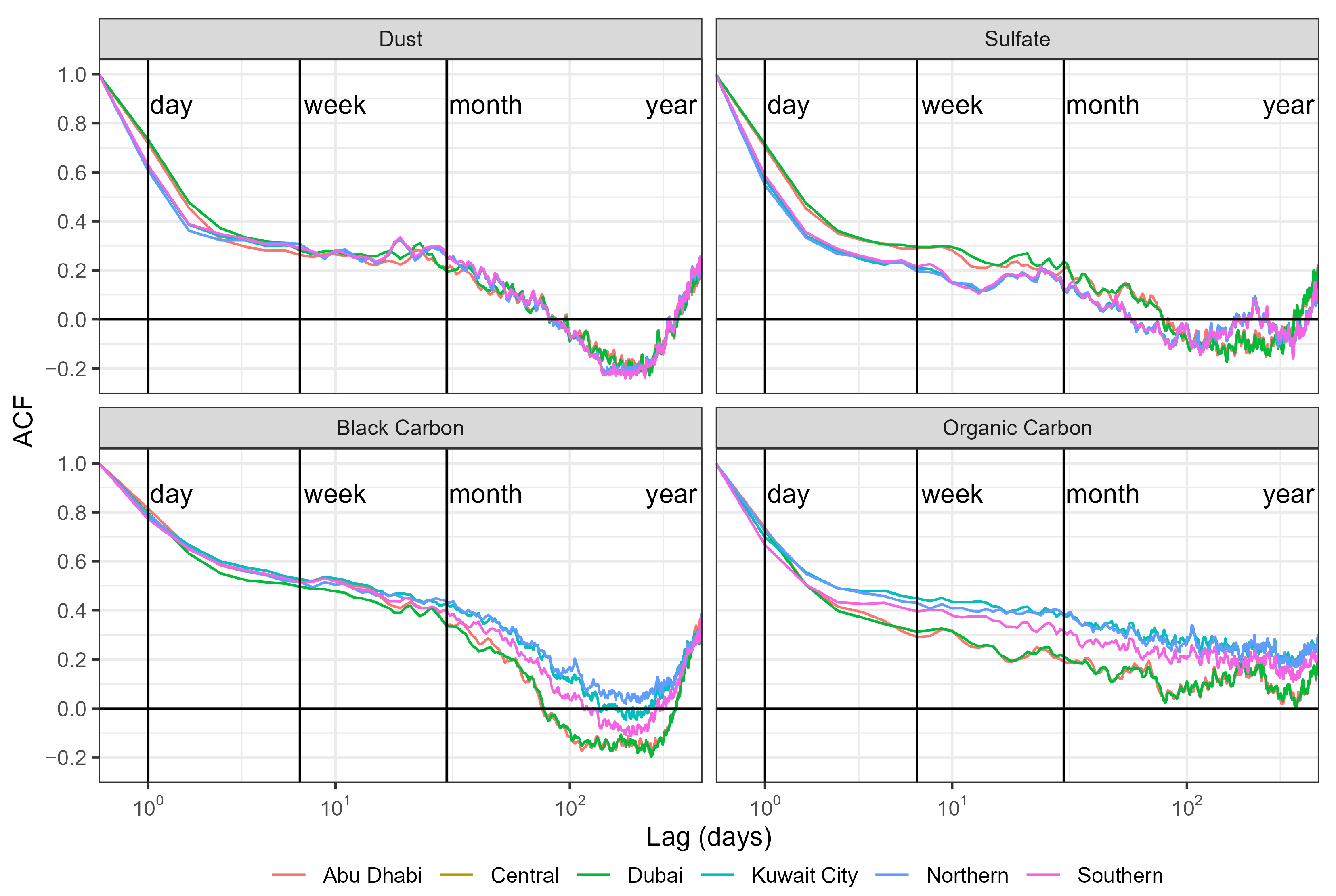
Among the assimilated aerosol MERRA-2 variables, the autocorrelation for dust extinction showed a small separation between PM sites in Kuwait and the U.A.E. early on, yet they all had an e-folding length at 3 days, after which there was little distinction between the two regions (Figure A3). Sulfate extinction showed clearer separation between the two regions for almost a month; the e-folding length was at 2 days for Kuwait sites and 3 days for the U.A.E. There was also little separation between Kuwait and the U.A.E. for black carbon extinction, and the e-folding length was just over a month for Kuwait and slightly under a month for the U.A.E.
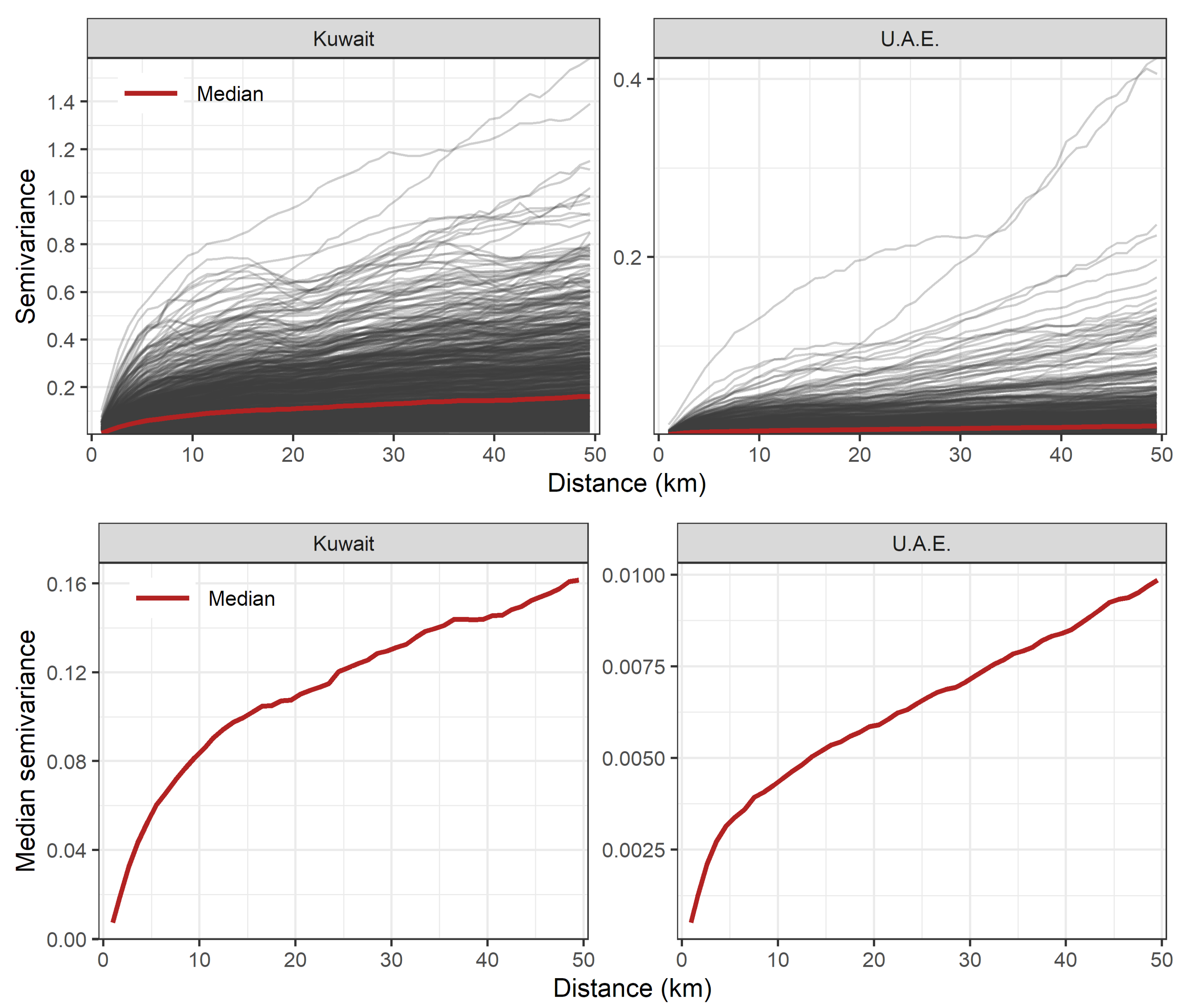
We restricted our analysis of spatial autocorrelation to days with at least 2500 successful AOD retrievals in each region. From 2017 through 2019, we analyzed daily semivariograms for 961 days in Kuwait ranging from 2515 to 19,552 AOD retrievals, with a median of 18,116 AOD retrievals per day. In the same period, we analyzed daily semivariograms for 1001 days in the U.A.E. ranging from 2610 to 23,609 AOD retrievals per day, with a median of 20,721 AOD retrievals per day. The top row of Figure 8 shows the daily semivariograms for each region, with the median semivariograms in red (note the y-axes are different for each region). In order to better show the aggregate trend of spatial autocorrelation, median semivariograms are shown in the bottom row of Figure 8.
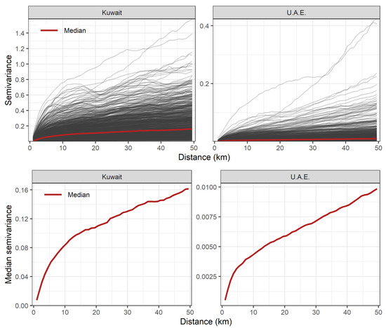
Figure 8.
Daily semivariograms for MAIAC AOD in Kuwait and the U.A.E. (grey lines in top row) and median semivariograms (red lines in both top and bottom rows).
Daily and median semivariograms of MAIAC AOD in Kuwait and the U.A.E. demonstrated clear differences in spatial autocorrelation trends between the two regions. Daily semivariograms in Kuwait showed greater semivariance and greater variation compared to the U.A.E. where semivariance was both smaller and demonstrated less variation. The median semivariograms showed that MAIAC AOD in Kuwait reached a partial sill at 0.1 with a range of 15 km while MAIAC AOD in the U.A.E. reached a partial sill at 0.004 with a range of 5 km. These semivariance trends showed that in the U.A.E. MAIAC AOD had much smaller spatial variability compared to Kuwait, even at distances as far as 50 km.
4. Discussion
In this study we applied methods developed in our previous work to estimate PM from satellite-observed AOD and meteorology over the Middle East, a geographic region with poor air quality and meteorological phenomena that render air quality estimation difficult. By noting regional differences in model performance, we explored possible statistical explanations including variable importance in the best fitting models as well as temporal and spatial autocorrelation trends in AOD and PM.
Model performance in Kuwait was similar to our previous study in Mongolia, although the Mongolia models did not include meteorology [38]. On the other hand, model performance in the U.A.E. was similar to the improved results we found modeling PM and PM speciation over California [29], which incorporated meteorology. We observed that the non-linear relationship between PM and satellite-retrieved AOD also affected the predictive performance of machine learning methods differently: gradient boosting, random forest, and support vector machines performed better than ridge and LASSO regression. Curiously, the linear methods did not perform much worse than GBM and RF in the U.A.E. and even outperformed SVM in the MISR AOD models (Table 1). These findings indicate that linear approaches should be carefully considered when constructing prediction models in other study regions.
The comparison between MAIAC AOD and MISR fractionated AODs also highlighted important differences. First, our data showed stronger linear correlation between PM and MISR AOD than MAIAC AOD ( and 0.38, respectively). Although the MAIAC models were developed on a data set with 4–6 times the sample size of the MISR models, their predictive performances were equivalent, both in the overall and the regional models (Table 1). MISR AOD also contributed more to the predictive accuracy of RF models (0.030–0.087% increases in MSE when excluded) compared to MAIAC AOD (0.009–0.044% increases in MSE when excluded). The MISR model in Kuwait saw greater improvements in predictive accuracy attributable to total and fractionated AODs, while the MISR model in the U.A.E. saw greater reliance on temporal (Julian date) and meteorological variables (temperature and UV radiation).
Similarly, while MAIAC AOD was less important than MERRA-2 dust, temperature, and month of the year in predicting PM over Kuwait, its importance was even smaller in the U.A.E. When we excluded AOD variables entirely from each model, the MAIAC-based models performed similarly while MISR-based models performed worse. Notably, the Kuwait model without MISR AODs observed the largest decrease in test (Figure 5), while the overall model predicted better in the U.A.E. without AOD variables.
The differences in predictive performance between Kuwait and the U.A.E. were part of a larger trend in our study where both the overall and the regional models performed differently depending on the region. The Kuwait models performed poorly in most configurations compared to the U.A.E. models despite having twice the sample size, indicating that sample size was not the only driver of the observed regional differences. Regional model performance differences were consistent with other PM studies where geography-based leave-one-out cross-validation revealed that one trained model did not perform the same everywhere. Di et al. (2019) obtained lower cross-validated in western subdivisions of the contiguous U.S., which could be attributed to the sparsity of PM monitors in these regions [5]. They also suggested that in mountainous regions such as the Appalachians and Rocky Mountains, terrain had an important influence on model performance.
Regional analyses of temporal and spatial autocorrelation further revealed significant heterogeneity. PM measurements in Kuwait demonstrated weak temporal autocorrelation (i.e., fast ACF decay), while PM in the U.A.E. showed slower autocorrelation decay (Figure 7). MAIAC AOD also showed a similar but smaller difference in temporal autocorrelation decay between the two regions. Anderson et al. (2003) observed different ACF trends in ground-monitored AOD from two AERONET stations (Bondville in Illinois and Spitzbergen in Norway) [44]. As the Abu Dhabi station was only active for very short periods during 2004–2005 and did not provide sufficient data, ACFs were calculated using MAIAC AOD instead. We observed different ACF trends with MAIAC AOD in the two regions, although the difference was negligible after 4 days. PM autocorrelation decayed much slower than AOD autocorrelation in the U.A.E., similar to findings by Kaku et al. (2018) in the Southeastern U.S. [25]. Regional semivariograms also demonstrated distinct differences in MAIAC AOD spatial autocorrelation trends: AOD in the U.A.E. showed smaller variance than in Kuwait, as far as 50 km (Figure 8). Slower temporal decay and greater spatial homogeneity may in part explain why the models performed better in the U.A.E. than in Kuwait.
Differences in spatial and temporal autocorrelation trends could explain some of the differences in variable importance between the regional models. For example, in the U.A.E. where PM showed stronger temporal autocorrelation, the model seemed to rely more on variables with similarly stronger temporal autocorrelation such as temperature and UV radiation (Figure A2), as well as temporal trends (Julian date), rather than satellite AOD, which showed poor temporal autocorrelation (Figure 7). On the other hand, in Kuwait where PM correlated poorly over time, the model relied less on meteorological variables and more on aerosol-related variables, including MERRA-2 extinctions (Figure A3).
These findings highlight the challenge of modeling PM over large areas that cover subregions with potentially heterogeneous temporal and spatial trends. Our regional models focused on two subregions with similar geographical characteristics: the Kuwait PM monitors covered an east-facing coastal region at approximately 40 km × 90 km, and the U.A.E. monitors covered a west-facing coastal region at approximately 85 km × 95 km. However, the two subregions showed very different trends in PM temporal dependence, which likely affected the predictive power of the respective regional models. The overall models with eight monitors in the study area also masked the difference in test in Kuwait (lower) and the U.A.E. (higher). Our study still found greater utility in models with larger spatial coverage when the data were available; regional models did not necessarily predict better than the overall model in their respective regions. We recommend careful evaluation of subregional spatial and temporal trends to better understand differences in inter-region predictive performance.
Finally, a test of model transferability demonstrated the difficulty of using models trained with data from one region to predict PM in another region. This approach was taken by Li et al. (2021) where their final model trained only on PM data in Kuwait was used to predict PM in neighboring Iraq [36]. In our study, the trained and tested Kuwait-based model was transferred 850 km southeast to similarly coastal U.A.E. with very poor performance. Therefore, we caution against using a model trained on data from one region to another, even if they have similar geographies. We do note that Li et al. (2021) used a multi-stage modeling framework that took advantage of the relatively stable relationship between visibility and PM, likely improving model transferability given the severe scarcity of reliable PM data in Iraq, which offered few modeling alternatives.
The largest limitation of this study is the small sample sizes used for analysis. Although the dimension of the overall MAIAC-AOD dataset was in the thousands and the PM monitors in our data covered a large region—from Baghdad to Dubai—more than half of the data were in Kuwait. We introduced spatial variation in the data by using coordinates of MAIAC pixels instead of PM monitors, but the small number of monitors meant that predictions relative to regions further away from these sites were likely less accurate, and the ability to capture local variability in PM was limited. While this could be ameliorated by the addition of air pollution monitors, retrospective prediction of historical PM measurement may remain unreliable.
Using assimilated meteorology and aerosol data at lower resolutions compared to the native resolutions of MAIAC and MISR was another limitation. This relates to spatial misalignment, specifically the change of support problem discussed by Gotway and Young (2002) as well as Banerjee et al. (2015) [45,46]. Downscaling gridded data is an active area of research with different interpolation approaches. For example, Li et al. (2020) recently downscaled MERRA-2 data from 50 km to 1 km using residual deep network [35]. In our context, such downscaling would not guarantee better prediction performance as our handful of PM monitors were largely located in urban areas with complex anthropogenic air pollution sources. Simple downscaling methods (e.g., bilinear interpolation) were likely to produce overly smoothed surfaces, while sophisticated methods (e.g., deep learning) result in difficult uncertainty quantification.
One shortcoming of our study concerned the general approach of relying on machine learning methods to predict PM, particularly non-parametric learners. Classical statistical models such as linear regression explicitly assume that the error term follows a particular distribution (e.g., Gaussian). Under this assumption, prediction uncertainty can be quantified in a parametric manner such as prediction intervals based on standard errors. However, non-parametric machine learning methods such as gradient boosting and random forest depend on hyper-parameters (such as number of trees and learning rate) that are typically chosen via non-statistical optimization methods such as cross-validation. As such, it is difficult to quantity uncertainty for prediction estimates from these learners. Several uncertainty quantification methods have been proposed, such as bootstrap sampling by Hastie et al. (2009) [39], yet few air pollution studies have reported uncertainty on their estimates. Predictions by Di et al. (2019), which covered the contiguous U.S., did include PM uncertainty estimates by modeling the monthly standard deviation of the difference between daily monitored and predicted PM at 1 km resolution [5].
5. Conclusions
Our study contributes to a large body of research that has established (1) remotely sensed AOD as a helpful addition to models estimating PM, particularly where PM monitors are scarce, and that (2) machine learning, notably non-linear techniques, is a powerful means of predicting PM using AOD and meteorology. In the overall models as well as separate regional models for Kuwait and the U.A.E., we observed heterogeneity in predictive performance across regions despite sharing key geographical features. Spatial and temporal autocorrelation trends for PM and MAIAC AOD revealed regional differences, and we suggest that these differences can help explain the discrepancies in model performance and feature importance between regions. Noting issues in model transferability, we also caution against applying regionally tuned models to different geographic areas.
PM data scarcity in the Middle East will continue to pose serious challenges to modeling efforts, yet understanding divergent spatial and temporal trends can better inform future work in this area and others.
Author Contributions
Conceptualization, M.F. and O.K.; methodology, K.C., M.F., O.K. and M.G.; formal analysis, K.C.; data curation, K.C., M.F. and H.L.; writing—original draft preparation, K.C. and M.F.; writing—review and editing, K.C. and M.F.; supervision, M.F. and O.K.; project administration, M.F.; funding acquisition, M.F. All authors have read and agreed to the published version of the manuscript.
Funding
This research was funded by National Aeronautics and Space Administration grant number 80NSSC19K0225.
Data Availability Statement
Analysis data will be available upon request.
Conflicts of Interest
The authors declare no conflict of interest.
Abbreviations
The following abbreviations are used in this manuscript:
| ACF | Autocorrelation Function; |
| AERONET | AErosol RObotic NETwork; |
| AOD | Aerosol Optical Depth; |
| BLH | Boundary Layer Height; |
| ERA5 | ECMWF Reanalysis, version 5; |
| HHI | Harvard High-capacity Impactors; |
| MAIAC | MultiAngle Implementation of Atmospheric Correction; |
| MERRA-2 | Modern-Era Retrospective analysis for Research and Applications, version 2; |
| MISR | Multiangle Imaging SpectroRadiometer; |
| MODIS | MODerate resolution Imaging Spectroradiometer; |
| MSE | Mean squared error; |
| RMSE | Root mean squared error. |
Appendix A
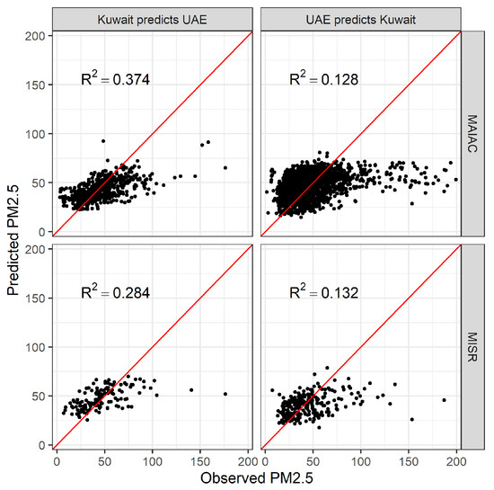
Figure A1.
Out-of-region PM predictions for Kuwait-trained models over the U.A.E. (left column) and out-of-region PM predictions for U.A.E.-trained models over Kuwait (right column) by MAIAC and MISR AODs (top and bottom rows, respective).
Figure A1.
Out-of-region PM predictions for Kuwait-trained models over the U.A.E. (left column) and out-of-region PM predictions for U.A.E.-trained models over Kuwait (right column) by MAIAC and MISR AODs (top and bottom rows, respective).
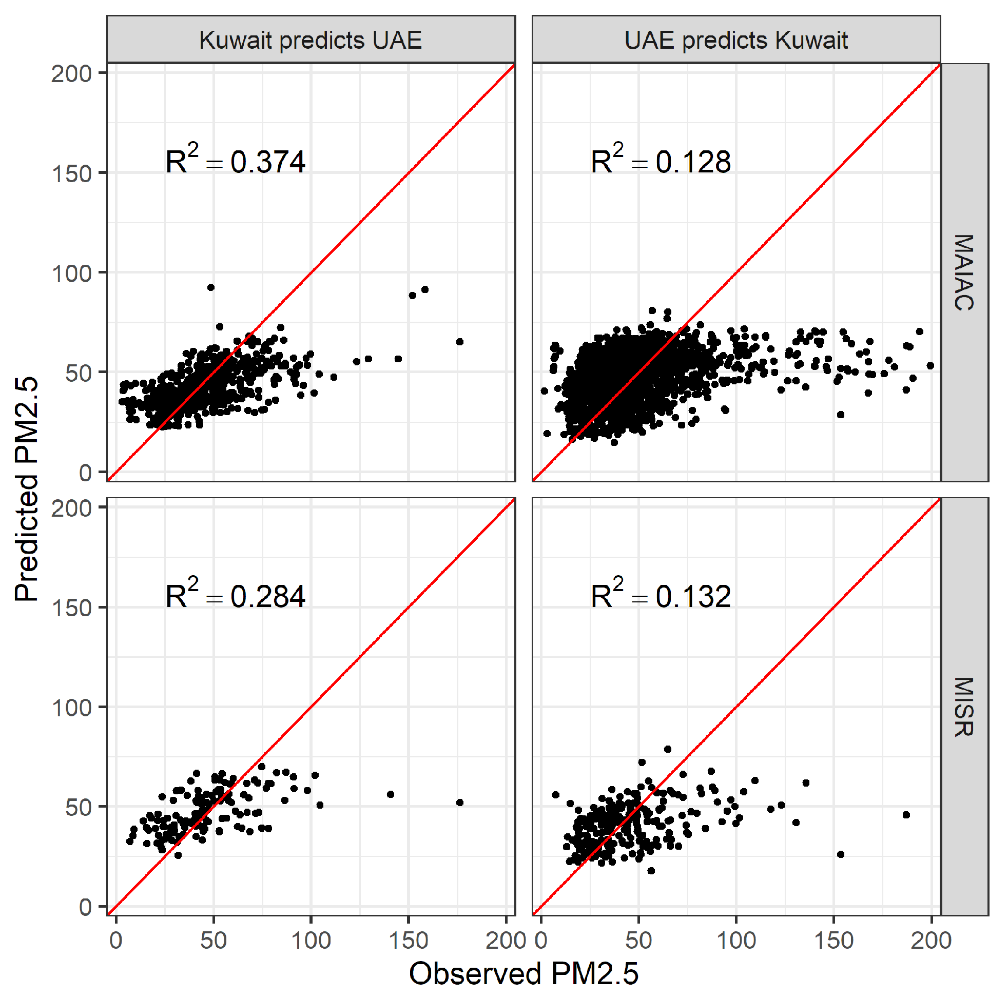
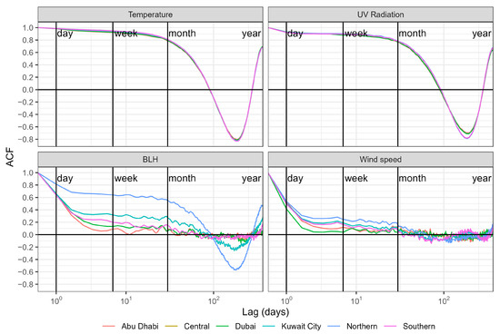
Figure A2.
Autocorrelation functions for ERA5 meteorological variables with high importance in the random forests models. The Kuwait City and Central monitors shared the same MERRA-2 pixel and, thus, the same ACF.
Figure A2.
Autocorrelation functions for ERA5 meteorological variables with high importance in the random forests models. The Kuwait City and Central monitors shared the same MERRA-2 pixel and, thus, the same ACF.
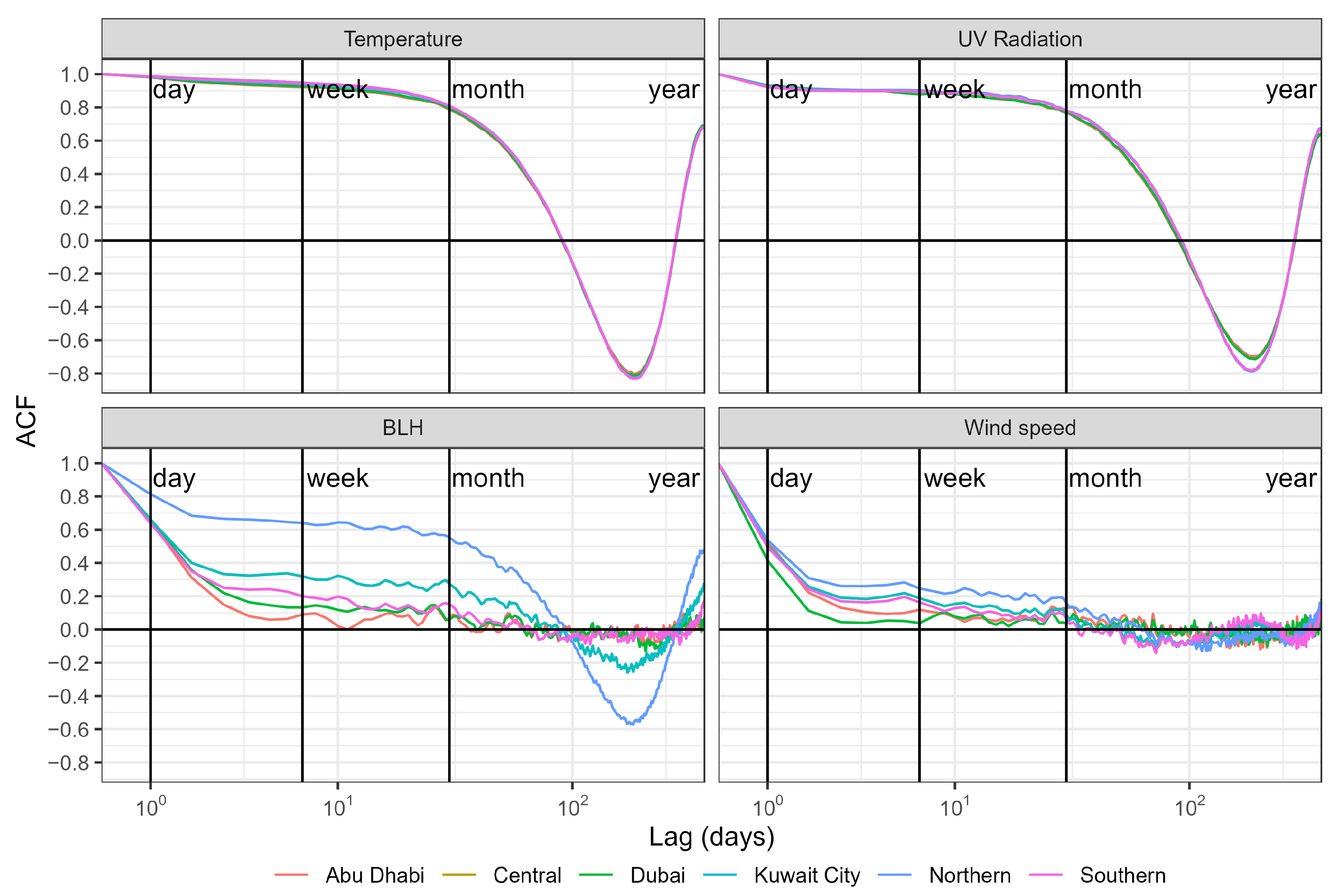
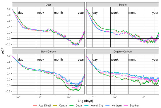
Figure A3.
Autocorrelation functions for MERRA-2 assimilated aerosol extinction variables, including dust, sulfate, black carbon, and organic carbon. The Kuwait City and Central monitors shared the same MERRA-2 pixel and, thus, the same ACF. Organic carbon was not found to be useful in any models and was excluded in the final PM models.
References
- Brauer, M.; Amann, M.; Burnett, R.T.; Cohen, A.; Dentener, F.; Ezzati, M.; Henderson, S.B.; Krzyzanowski, M.; Martin, R.V.; Dingenen, R.V.; et al. Exposure Assessment for Estimation of the Global Burden of Disease Attributable to Outdoor Air Pollution. Environ. Sci. Technol. 2012, 46, 652–660. [Google Scholar] [CrossRef] [Green Version]
- de Sherbinin, A.; Levy, M.A.; Zell, E.; Weber, S.; Jaiteh, M. Using satellite data to develop environmental indicators. Environ. Res. Lett. 2014, 9, 084013. [Google Scholar] [CrossRef]
- van Donkelaar, A.; Martin, R.V.; Brauer, M.; Boys, B.L. Use of Satellite Observations for Long-Term Exposure Assessment of Global Concentrations of Fine Particulate Matter. Environ. Health Perspect. 2015, 123, 135–143. [Google Scholar] [CrossRef] [Green Version]
- Shaddick, G.; Thomas, M.L.; Green, A.; Brauer, M.; Donkelaar, A.; Burnett, R.; Chang, H.H.; Cohen, A.; Dingenen, R.V.; Dora, C.; et al. Data integration model for air quality: A hierarchical approach to the global estimation of exposures to ambient air pollution. J. R. Stat. Soc. Ser. Appl. Stat. 2018, 67, 231–253. [Google Scholar] [CrossRef]
- Di, Q.; Amini, H.; Shi, L.; Kloog, I.; Silvern, R.; Kelly, J.; Sabath, M.B.; Choirat, C.; Koutrakis, P.; Lyapustin, A.; et al. An ensemble-based model of PM2.5 concentration across the contiguous United States with high spatiotemporal resolution. Environ. Int. 2019, 130, 104909. [Google Scholar] [CrossRef]
- van Donkelaar, A.; Martin, R.V.; Li, C.; Burnett, R.T. Regional Estimates of Chemical Composition of Fine Particulate Matter Using a Combined Geoscience-Statistical Method with Information from Satellites, Models, and Monitors. Environ. Sci. Technol. 2019, 53, 2595–2611. [Google Scholar] [CrossRef] [PubMed] [Green Version]
- Garay, M.J.; Kalashnikova, O.V.; Bull, M.A. Development and assessment of a higher-spatial-resolution (4.4 km) MISR aerosol optical depth product using AERONET-DRAGON data. Atmos. Chem. Phys. 2017, 17, 5095–5106. [Google Scholar] [CrossRef] [Green Version]
- Lyapustin, A.; Wang, Y.; Korkin, S.; Huang, D. MODIS Collection 6 MAIAC algorithm. Atmos. Meas. Tech. 2018, 11, 5741–5765. [Google Scholar] [CrossRef] [Green Version]
- Liang, F.; Xiao, Q.; Wang, Y.; Lyapustin, A.; Li, G.; Gu, D.; Pan, X.; Liu, Y. MAIAC-based long-term spatiotemporal trends of PM2.5 in Beijing, China. Sci. Total Environ. 2018, 616, 1589–1598. [Google Scholar] [CrossRef] [PubMed]
- Wang, W.; Zhao, S.; Jiao, L.; Taylor, M.; Zhang, B.; Xu, G.; Hou, H. Estimation of PM2.5 Concentrations in China Using a Spatial Back Propagation Neural Network. Sci. Rep. 2019, 9, 13788. [Google Scholar] [CrossRef] [Green Version]
- Tsiouri, V.; Kakosimos, K.E.; Kumar, P. Concentrations, sources and exposure risks associated with particulate matter in the Middle East Area—A review. Air Qual. Atmos. Health 2015, 8, 67–80. [Google Scholar] [CrossRef]
- Alahmad, B.; Al-Hemoud, A.; Kang, C.M.; Almarri, F.; Kommula, V.; Wolfson, J.M.; Bernstein, A.S.; Garshick, E.; Schwartz, J.; Koutrakis, P. A two-year assessment of particulate air pollution and sources in Kuwait. Environ. Pollut. 2021, 282, 117016. [Google Scholar] [CrossRef]
- Council, N.R. Review of the Department of Defense Enhanced Particulate Matter Surveillance Program Report; National Academies Press: Washington, DC, USA, 2010. [Google Scholar]
- Kloog, I.; Koutrakis, P.; Coull, B.A.; Lee, H.J.; Schwartz, J. Assessing temporally and spatially resolved PM2.5 exposures for epidemiological studies using satellite aerosol optical depth measurements. Atmos. Environ. 2011, 45, 6267–6275. [Google Scholar] [CrossRef]
- Franklin, M.; Vora, H.; Avol, E.; McConnell, R.; Lurmann, F.; Liu, F.; Penfold, B.; Berhane, K.; Gilliland, F.; Gauderman, W.J. Predictors of intra-community variation in air quality. J. Expo. Sci. Environ. Epidemiol. 2012, 22, 135–147. [Google Scholar] [CrossRef] [PubMed] [Green Version]
- van Donkelaar, A.; Martin, R.V.; Spurr, R.J.D.; Burnett, R.T. High-Resolution Satellite-Derived PM2.5 from Optimal Estimation and Geographically Weighted Regression over North America. Environ. Sci. Technol. 2015, 49, 10482–10491. [Google Scholar] [CrossRef]
- Zheng, Y.; Zhang, Q.; Liu, Y.; Geng, G.; He, K. Estimating ground-level PM2.5 concentrations over three megalopolises in China using satellite-derived aerosol optical depth measurements. Atmos. Environ. 2016, 124, 232–242. [Google Scholar] [CrossRef]
- Franklin, M.; Kalashnikova, O.V.; Garay, M.J. Size-resolved particulate matter concentrations derived from 4.4 km-resolution size-fractionated Multi-angle Imaging SpectroRadiometer (MISR) aerosol optical depth over Southern California. Remote Sens. Environ. 2017, 196, 312–323. [Google Scholar] [CrossRef]
- Sorek-Hamer, M.; Franklin, M.; Chau, K.; Garay, M.; Kalashnikova, O. Spatiotemporal Characteristics of the Association between AOD and PM over the California Central Valley. Remote Sens. 2020, 12, 685. [Google Scholar] [CrossRef] [Green Version]
- Engel-Cox, J.A.; Holloman, C.H.; Coutant, B.W.; Hoff, R.M. Qualitative and quantitative evaluation of MODIS satellite sensor data for regional and urban scale air quality. Atmos. Environ. 2004, 38, 2495–2509. [Google Scholar] [CrossRef]
- Hammer, M.S.; van Donkelaar, A.; Li, C.; Lyapustin, A.; Sayer, A.M.; Hsu, N.C.; Levy, R.C.; Garay, M.J.; Kalashnikova, O.V.; Kahn, R.A.; et al. Global Estimates and Long-Term Trends of Fine Particulate Matter Concentrations (1998–2018). Environ. Sci. Technol. 2020, 54, 7879–7890. [Google Scholar] [CrossRef]
- Sullivan, R.; Pryor, S. Quantifying spatiotemporal variability of fine particles in an urban environment using combined fixed and mobile measurements. Atmos. Environ. 2014, 89, 664–671. [Google Scholar] [CrossRef]
- Sullivan, R.; Levy, R.; Pryor, S. Spatiotemporal coherence of mean and extreme aerosol particle events over eastern North America as observed from satellite. Atmos. Environ. 2015, 112, 126–135. [Google Scholar] [CrossRef]
- Toth, T.D.; Zhang, J.; Reid, J.S.; Vaughan, M.A. A bulk-mass-modeling-based method for retrieving particulate matter pollution using CALIOP observations. Atmos. Meas. Tech. 2019, 12, 1739–1754. [Google Scholar] [CrossRef] [Green Version]
- Kaku, K.C.; Reid, J.S.; Hand, J.L.; Edgerton, E.S.; Holben, B.N.; Zhang, J.; Holz, R.E. Assessing the Challenges of Surface-Level Aerosol Mass Estimates From Remote Sensing During the SEAC4RS and SEARCH Campaigns: Baseline Surface Observations and Remote Sensing in the Southeastern United States. J. Geophys. Res. Atmos. 2018, 123, 7530–7562. [Google Scholar] [CrossRef] [Green Version]
- Brown, K.W.; Bouhamra, W.; Lamoureux, D.P.; Evans, J.S.; Koutrakis, P. Characterization of Particulate Matter for Three Sites in Kuwait. J. Air Waste Manag. Assoc. 2008, 58, 994–1003. [Google Scholar] [CrossRef]
- Masri, S.; Garshick, E.; Coull, B.A.; Koutrakis, P. A novel calibration approach using satellite and visibility observations to estimate fine particulate matter exposures in Southwest Asia and Afghanistan. J. Air Waste Manag. Assoc. 2016, 67, 86–95. [Google Scholar] [CrossRef] [PubMed]
- OpenAQ. Available online: https://openaq.org (accessed on 11 January 2021).
- Chau, K.; Franklin, M.; Gauderman, W.J. Satellite-Derived PM2.5 Composition and Its Differential Effect on Children’s Lung Function. Remote Sens. 2020, 12, 1028. [Google Scholar] [CrossRef] [Green Version]
- Hersbach, H.; Bell, B.; Berrisford, P.; Hirahara, S.; Horányi, A.; Muñoz-Sabater, J.; Nicolas, J.; Peubey, C.; Radu, R.; Schepers, D.; et al. The ERA5 global reanalysis. Q. J. R. Meteorol. Soc. 2020, 146, 1999–2049. [Google Scholar] [CrossRef]
- Smith, D.M.; Booth, B.B.B.; Dunstone, N.J.; Eade, R.; Hermanson, L.; Jones, G.S.; Scaife, A.A.; Sheen, K.L.; Thompson, V. Role of volcanic and anthropogenic aerosols in the recent global surface warming slowdown. Nat. Clim. Chang. 2016, 6, 936–940. [Google Scholar] [CrossRef]
- Freychet, N.; Tett, S.F.B.; Bollasina, M.; Wang, K.C.; Hegerl, G.C. The Local Aerosol Emission Effect on Surface Shortwave Radiation and Temperatures. J. Adv. Model. Earth Syst. 2019, 11, 806–817. [Google Scholar] [CrossRef]
- Gelaro, R.; McCarty, W.; Suárez, M.J.; Todling, R.; Molod, A.; Takacs, L.; Randles, C.A.; Darmenov, A.; Bosilovich, M.G.; Reichle, R.; et al. The Modern-Era Retrospective Analysis for Research and Applications, Version 2 (MERRA-2). J. Clim. 2017, 30, 5419–5454. [Google Scholar] [CrossRef]
- Bosilovich, M.G.; Lucchesi, R.; Suárez, M.J. MERRA-2: File Specification. GMAO Office Note No. 9 (Version 1.1). Available online: http://gmao.gsfc.nasa.gov/pubs/office_notes (accessed on 11 January 2021).
- Li, L.; Girguis, M.; Lurmann, F.; Pavlovic, N.; McClure, C.; Franklin, M.; Wu, J.; Oman, L.D.; Breton, C.; Gilliland, F.; et al. Ensemble-based deep learning for estimating PM2.5 over California with multisource big data including wildfire smoke. Environ. Int. 2020, 145, 106143. [Google Scholar] [CrossRef]
- Li, J.; Garshick, E.; Hart, J.E.; Li, L.; Shi, L.; Al-Hemoud, A.; Huang, S.; Koutrakis, P. Estimation of ambient PM2.5 in Iraq and Kuwait from 2001 to 2018 using machine learning and remote sensing. Environ. Int. 2021, 151, 106445. [Google Scholar] [CrossRef]
- Holben, B.; Eck, T.; Slutsker, I.; Tanré, D.; Buis, J.; Setzer, A.; Vermote, E.; Reagan, J.; Kaufman, Y.; Nakajima, T.; et al. AERONET—A Federated Instrument Network and Data Archive for Aerosol Characterization. Remote Sens. Environ. 1998, 66, 1–16. [Google Scholar] [CrossRef]
- Franklin, M.; Chau, K.; Kalashnikova, O.; Garay, M.; Enebish, T.; Sorek-Hamer, M. Using Multi-Angle Imaging SpectroRadiometer Aerosol Mixture Properties for Air Quality Assessment in Mongolia. Remote Sens. 2018, 10, 1317. [Google Scholar] [CrossRef] [Green Version]
- Hastie, T.; Tibshirani, R.; Friedman, J. The Elements of Statistical Learning: Data Mining, Inference, and Prediction; Springer: New York, NY, USA, 2009. [Google Scholar]
- Sorek-Hamer, M.; Strawa, A.; Chatfield, R.; Esswein, R.; Cohen, A.; Broday, D. Improved retrieval of PM2.5 from satellite data products using non-linear methods. Environ. Pollut. 2013, 182, 417–423. [Google Scholar] [CrossRef] [PubMed]
- Kloog, I.; Nordio, F.; Coull, B.A.; Schwartz, J. Incorporating Local Land Use Regression And Satellite Aerosol Optical Depth in A Hybrid Model of Spatiotemporal PM2.5 Exposures in the Mid-Atlantic States. Environ. Sci. Technol. 2012, 46, 11913–11921. [Google Scholar] [CrossRef] [Green Version]
- Strobl, C.; Boulesteix, A.L.; Zeileis, A.; Hothorn, T. Bias in random forest variable importance measures: Illustrations, sources and a solution. BMC Bioinform. 2007, 8, 25. [Google Scholar] [CrossRef] [Green Version]
- Franklin, M.; Kalashnikova, O.; Garay, M.; Fruin, S. Characterization of Subgrid-Scale Variability in Particulate Matter with Respect to Satellite Aerosol Observations. Remote Sens. 2018, 10, 623. [Google Scholar] [CrossRef] [Green Version]
- Anderson, T.L.; Charlson, R.J.; Winker, D.M.; Ogren, J.A.; Holmén, K. Mesoscale Variations of Tropospheric Aerosols. J. Atmos. Sci. 2003, 60, 119–136. [Google Scholar] [CrossRef]
- Gotway, C.A.; Young, L.J. Combining Incompatible Spatial Data. J. Am. Stat. Assoc. 2002, 97, 632–648. [Google Scholar] [CrossRef] [Green Version]
- Banerjee, S.; Carlin, B.P.; Gelfand, A.E. Hierarchical Modeling and Analysis for Spatial Data; CRC Press, Taylor & Francis Group: Boca Raton, FL, USA, 2015. [Google Scholar]
Publisher’s Note: MDPI stays neutral with regard to jurisdictional claims in published maps and institutional affiliations. |
© 2021 by the authors. Licensee MDPI, Basel, Switzerland. This article is an open access article distributed under the terms and conditions of the Creative Commons Attribution (CC BY) license (https://creativecommons.org/licenses/by/4.0/).

