Abstract
The vegetation of the Qinghai–Tibet Plateau (QTP) is vital to the global climate change and ecological security of China. However, the impact of climate variation on the spatial pattern and zonal distribution of vegetation in the QTP remains unclear. Accordingly, we used multisource remote-sensing vegetation indices (GIMMS-LAI, GIMMS NDVI, GLOBMAP LAI, MODIS EVI, MODIS NDVI, and MODIS NIRv), climate data, a digital elevation model, and the moving window method to investigate the changes in vegetation greenness and its response to climate variations in the QTP from 2001 to 2016. Results showed that the vegetation was greening in the QTP, which might be attributed to the increases in temperature and radiation. By contrast, the browning of vegetation may be caused by drought. Notably, the spatial patterns of vegetation greenness and its variations were linearly correlated with climate at low altitudes, and vegetation greenness was non-linearly correlated with climate at high altitudes. The Northwestern QTP needs to be focused on in regard to positive and decreased VGEG (vegetation greenness along the elevation gradient). The significantly positive VGEG was up to (34.37 ± 2.21) % of the QTP, which indicated a homogenization of vegetation greenness on elevation. This study will help us to understand the spatial distribution of vegetation greenness and VGEG in the QTP under global warming, and it will benefit ecological environment management, policymaking, and future climate and carbon sink (source) prediction.
1. Introduction
The accelerating global warming and carbon dioxide (CO2) concentration have exerted widespread impacts on the terrestrial ecosystem in the past three decades [1,2,3], the impact of which on vegetation dynamics may be more pronounced in high mountainous areas [4,5]. Vegetation plays a crucial role in mitigation of global climate [6]; vegetation greenness generally decreases with the increased elevation, because the low temperature limits the growth of vegetation in high altitudes [7], which indicates a negative vegetation greenness along the elevation gradient (VGEG can be defined as the regression value between vegetation greenness and elevation gradient in a certain extent). Growing evidence demonstrated that the warming rate is intensified in mountain environments [5,8,9,10], and this is likely to cause a completely different distribution of vegetation greenness on the altitude gradient [11]. However, the vegetation changes in high mountainous areas have not been unanimously concluded yet. Consequently, the elevation pattern of vegetation greenness may have changed in mountainous regions under the influence of global warming, because the warming rate in high-altitude areas is often greater than that in low-altitude areas [4,12]. Therefore, a scientific question is raised here of whether the pattern of vegetation greenness is altered in high mountainous areas along the altitude gradient.
The Qinghai–Tibet Plateau (QTP) is a unique geographical unit on the Earth, and it is known as the “third pole” of the Earth. The QTP has a crucial role in the ecological security of China [13] and the global carbon cycle [14,15]. The QTP is approximately 2.5 million km2, and it accounts for nearly 25% of the area of China. The grassland ecosystem of the QTP is extremely sensitive to climate variation and human activities because of its vulnerable ecosystem and the severe environments in the region [16,17]. So far, there are growing studies on the changes in vegetation along elevation in the alpine ecosystems, e.g., the QTP. However, the conclusions of existing studies are dramatically opposite [7,18,19]. The reasons can be summarized into the following points. On the timescale, the conclusions reached in different research periods do not support each other. Even if the two research phases are very close, the conclusions may be quite different. On the spatial scale, it is difficult to reach a consensus on research conclusions in different geographic locations, due to the heterogeneity of geographic space and its many influencing factors. In terms of research methods, it mainly includes field surveys and remote sensing. However, the spatial scales of the two methods are completely different, so it is not surprising that the research results are inconsistent. Remote sensing provides us with a wide range of perspectives to explore the distribution and changes of vegetation under the influence of climate. However, the use of a single remote-sensing data source is likely to ignore its own uncertainty in data acquisition, i.e., a single vegetation index (VI). Sensor design, photographing capability, noise processing, spatiotemporal resolution, etc., all contribute to the uncertainty. The utilization of multisource remote-sensing data can assess the uncertainty of vegetation greenness distribution and variation, which is also of great significance for exploring the impact of climate on vegetation. However, most of the conclusions come from a single remote-sensing data source [9,19,20,21,22].
Researchers have reached a broad consensus on vegetation greening in the past 30 years; that is, the CO2 fertilization effect plays a crucial role [23]. Human land use is a dominant driver of global greening after 2000, and it mainly occurs in China and India [24]. However, the changes in its spatial patterns are also highly uncertain at the global scale, especially for the years after 2000 [25]. Even if we have found that the changes in vegetation greenness have large discrepancies by using multisource VI in the hinterland of the QTP from 2001 to 2016 [26], the regularity of VGEG variation and the influencing factors that determine the altitude distribution of vegetation greenness have not been found. Moreover, a comprehensive study on the changes in the zonal distribution of vegetation greenness in the QTP is still lacking.
Considering the ecological importance of the QTP, and the defects and gaps in current scientific research, we selected the QTP as the study area, six kinds of remote-sensing-based VI and digital elevation model (DEM) data were utilized to identify the trend of vegetation greenness, to verify whether the spatial pattern of VGEG has been altered under climate variation, and to determine the effect of climate variation on the changes in the vegetation greenness and its elevational distribution from 2000 to 2016. This research will help us assess the impact of climate change on the vegetation of the QTP, formulate mitigation strategies for climate change, improve the carbon cycle model, and predict future vegetation changes and spatial distribution.
2. Materials and Methods
2.1. Study Area
The QTP is located in Western China (73.50–104.67° E, 25.99–39.83° N), and it covers more than 2.56 × 10⁶ km2 of area (Figure 1). Around 40% of the world’s population depends on, or is influenced by, the rivers that originate from the QTP [27]. Alpine meadows (38%) and alpine steppes (29%) are the dominant vegetation types in the QTP [28]. The meteorological dataset (see Section 2.3) indicated that the mean annual temperature is lower than −20 °C in the coldest region and higher than 20 °C in the warmest region in the QTP from 2001 to 2016 [29,30]. The QTP has experienced significant warming since the mid-1950s, with the mean annual temperature increasing by 0.3 °C per decade [14]. The Southeast QTP is the wettest area, with annual precipitation of over 1000 mm. Meanwhile, annual precipitation in the driest northwest area is less than 50 mm [31].
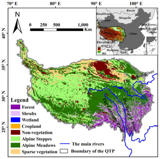
Figure 1.
Location of the QTP in China. The color map of the upper-right inset shows the elevation of the QTP. The main map presents the vegetation types of the QTP.
2.2. Remote-Sensing-Derived VI Datasets
The basic information of the remote-sensing-derived VI datasets is shown in Table 1. NDVI (Normalized Difference Vegetation Index) is a good indicator of vegetation growth status and spatial distribution density of vegetation, and it is directly related to vegetation distribution density and photosynthetic capacity [32]. GIMMS (Global Inventory Modeling and Mapping Studies) NDVI was derived from the AVHRR (Advanced Very High-Resolution Radiometer) sensor mounted on NOAA (National Oceanic and Atmospheric Administration) series satellites. The current GIMMS-NDVI data’s quality in high-latitude areas was significantly improved compared to the previous version [33].

Table 1.
Remote-sensing-derived VI datasets used in this study.
LAI (Leaf Area Index) is defined as the one-sided green leaf area per unit vegetated ground area in broadleaf canopies and as one-half the total needle surface area per unit vegetated ground area in coniferous canopies [34]. GIMMS-LAI data were generated by using FFNN (feedforward neural network) algorithm, which is based on the GIMMS-NDVI and the Moderate Resolution Imaging Spectroradiometer (MODIS) LAI data [34]. Global Mapping (GLOBMAP) LAI version 3 dataset was generated by MODIS and AVHRR data. The relationships between the AVHRR simple ratio and the MODIS LAI were established during the overlapped period (2000–2006). Then, the pixel-based relationship was used to estimate historical AVHRR LAI (1981–2000). Historical AVHRR LAI and MODIS LAI constitute the GLOBMAP LAI data on the entire time sequence (1981–2017) [35].
The monthly MODIS VI product (MOD13A3, Collection 6) includes NDVI and Enhanced VI (EVI). The enhanced vegetation index (EVI) was developed to optimize the vegetation signal with improved sensitivity in high biomass regions and improved vegetation monitoring through a de-coupling of the canopy background signal and a reduction in atmosphere influences [36].
The near-infrared reflectance of vegetation (NIRv) is the product of NIR reflectance and NDVI. NIRv is found to be strongly correlated with chlorophyll fluorescence and site-level gross primary productivity [37]. The temporal and spatial resolutions of NIRv are consistent with MODIS NDVI and EVI.
In summary, the spatial resolution of all VI data was interpolated to 0.01° (≈1.1 km) by using the bicubic interpolation method to keep consistent with MODIS VI data (the original resolution is 1 km). The study period of this work was set from 2001 to 2016 to facilitate the comparative research, because MODIS VI data started in 2001, and GIMMS VI data were only updated to 2016. At last, we used the maximum value composite method [38] to merge the original 15- and 8-day data into annual data for further analysis.
2.3. Climate Datasets
The climate datasets of China were derived from the National Tibetan Plateau Data Center (https://data.tpdc.ac.cn/en/. Accessed on 12 September 2021). The original climate data, including monthly temperature, precipitation, and radiation with a spatial resolution of 0.1° × 0.1°, cover the period of 1979–2018 [29]. The cubic interpolation method was used to resample the data to a spatial resolution of 0.01° × 0.01°. We further composited the monthly data to mean annual temperature (MAT), precipitation (MAP), and radiation (MAR) raster data, and then we extracted the raster data within the QTP from 2001 to 2016.
2.4. Calculation of the VGEG
The DEM data were obtained from the Shuttle Radar Topographic Mission, with a spatial resolution of 0.008° (≈1 km). We resampled the spatial resolution of DEM to 0.01° to be consistent with VI and climate data. The VGEG was calculated in three steps [9,26]. Step 1: We determined the size of the moving window, which determines the amount of data used for analysis for each move (the unit of each move is one pixel). The size of the moving window must ensure that we can obtain enough valid data for linear regression analysis. We recommend choosing the window size of 9 × 9 for calculation based on our experience. Step 2: We obtained two datasets by moving windows (e.g., one moving window extracts the VI, and the other extracts the DEM); each dataset contains 81 data (9 × 9 moving window). We then arranged them in order to prepare for analysis (Figure 2). Step 3: We performed linear regression analysis on the two sets of data, assigned the slope to the central moving window, and then traversed the entire study area to obtain VGEG. The statistical significance of the slope is tested by T-test. The moving window method can quickly traverse DEM and VI data, and perform data analysis within a fixed window range, so that the climate factors are relatively consistent. In addition, we used linear regression to analyze the change of vegetation greenness on the elevation gradients. Essentially, the regression value was solved by the least square method (see Section 2.5).
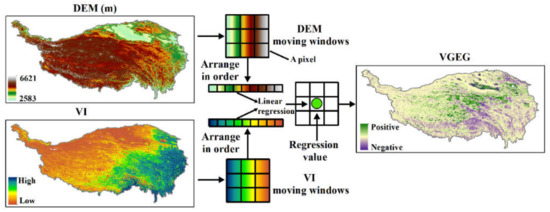
Figure 2.
Diagram of the calculation of VGEG. Here, we take a 3 × 3 window as an example.
2.5. Trend Analysis
Least squares method is a mathematical optimization technique. It finds the best function match of the data by minimizing the sum of squared errors. The polynomial line fitting of the least squares method is to find the best slope based on given data points. The slope is the trend of variables. We used the ordinary least squares method [39,40,41,42] to determine the trends in climate, VI, and VGEG in time series:
where VAR can be MAT, MAP, and MAR; each of the six Vis; and VGEG in this study. Moreover, i is the sequence number of the year (from 2001 to 2016), and n represents the total number of years. The significance of the trend was determined by the t-test.
2.6. Correlation Analysis
Pearson correlation coefficient is used to measure whether two datasets are on a line; its value is between −1 and 1. In the field of natural sciences, this coefficient is widely used to measure the degree of correlation between two variables [43]. We use Pearson correlation analysis to calculate the correlation between VIs and climate factors (MAT, MAP, and MAR). The correlation coefficient (r) of the two variables can be calculated by Equation (2).
The correlation coefficient between VI and MAT was taken as an example. Variables xi and yi denote the VI and MAT in year i, respectively; and x and y are the mean value of VI and MAT from 2001 to 2016.
3. Results
3.1. Trends and Spatial Patterns of Climate Factors and Their Elevational Distributions
MAT and MAR increased at rates of 0.02 °C/year and 8.26 MJ/m2/year, and the trend of MAR reached a significance level of 0.05. By contrast, the MAP showed a decreasing trend (−1.64 mm/year) in the study period (Figure 3a). The slope of MAT appeared to increase first from 2000 m (above sea level, similarly hereinafter) to 3300 m and then decreased sharply. Next, it remained stable from around 4000 to 6000 m. Finally, it showed an increasing trend above 6000 m (Figure 3b). MAP was found to decrease from 2000 to 3300 m, showed an increase around 3300 m, and remained stable between 5000 m and the higher elevation. The slope of MAP showed a slightly decreasing trend at low altitudes, and then, it exhibited sharp increases first and then decreases that took the elevation of 3300 m as the inflection point. Since then, the slope of MAP experienced some fluctuations with a slight downward trend (Figure 3c). The MAR showed an increasing trend from the elevation of 2000 to 3300 m, and then it decreased first and then increased at the altitudes above 3300 m. By contrast, the slope of MAR decreased drastically from 2000 to 3300 m, and then it exhibited a fluctuating increasing trend (Figure 3d).
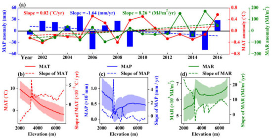
Figure 3.
Trend of the MAT, MAP, and MAR anomaly (a) and their mean value (solid curves) and slope (dashed curves) in elevation gradients (b–d) in the QTP from 2001 to 2016. The dashed straight lines denote the trend lines in (a). Asterisk (*) denotes that the slope is statistically significant at the 0.05 level. The colored shadow regions represent one standard deviation.
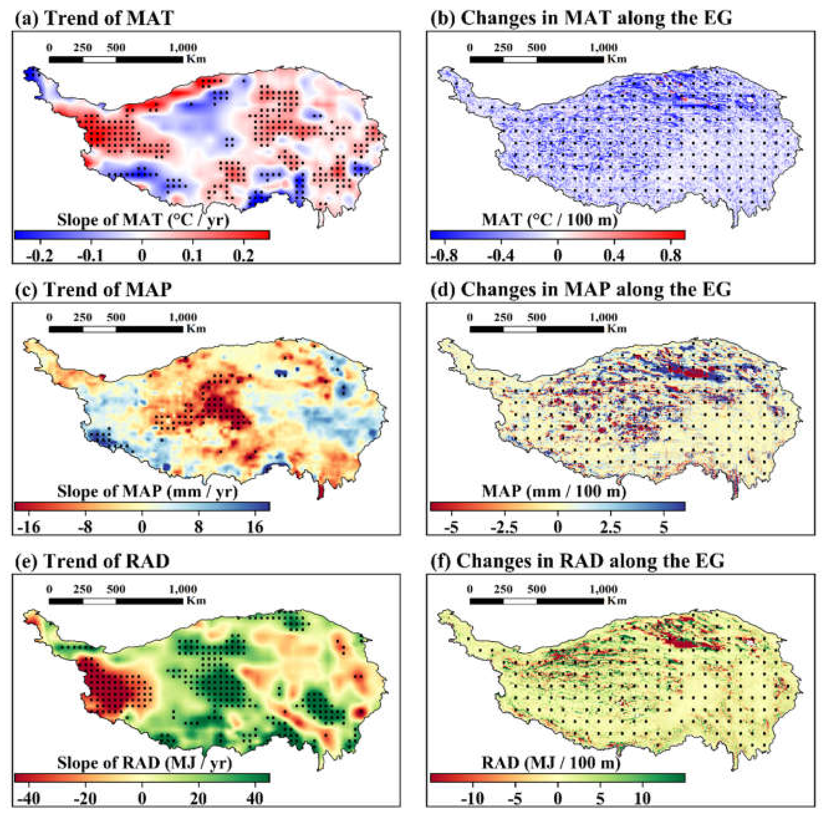
The spatial pattern of the MAT trend showed that nearly 63.18% of the study areas presented an increasing trend from 2001 to 2016, and 26.83% of the MAT reached a significance level of 0.05 (Figure 4a). By contrast, the regions with a decreasing trend of MAT occupied 36.82% of the study areas, and 9.06% of them were statistically significant. The positive changes in MAT along elevation gradients only accounted for 11.06% of the total study area (Figure 4b). As we know, MAT decreases with the increases in elevation, which can be reflected by a negative regression of MAT with elevation; the negative changes in MAT along elevation gradients were up to 88.94%, and 77.10% of the areas were statistically significant. This finding indicated that the method used in this study can capture the basic law that temperature decreases with the increase in elevation. The areas with a decreasing trend of MAP (58.32%) were larger than those with an increasing trend (41.68%). The regions with a significant decreasing trend accounted for 26.83%, and they were found in the center of the QTP. By contrast, the areas that reached a significant increasing trend only occupied 9.06%, and they were mainly distributed in the Western QTP (Figure 4c). The positive changes in MAP along the elevation gradient were scattered across the Western and Central QTP (Figure 4d). These regions accounted for 56.66% of the total study areas, and 42.14% of the area reached a significant positive level. Approximately 43.34% of the areas exhibited negative changes in MAP along elevation gradients, and the significant areas accounted for 29.76%. The MAR generally showed an increasing trend in the QTP (65.47% of the QTP), and 25.16% of them were statistically significant; they were mainly identified in the center of the QTP (Figure 4e). By contrast, the regions with a decreasing trend of MAR were mainly found in the Western QTP and a small part of Eastern QTP, and 9.47% of them reached a significance level of 0.05. The positive and negative changes in MAR along the elevation gradient accounted for 60.70% and 39.30% of the QTP, respectively.

Figure 4.
Spatial patterns of the climate trend and their changes along elevation gradients in the QTP from 2001 to 2016. (a,c,e) Trend of MAT, MAP, and MAR, respectively. (b,d,f) Changes in MAT, MAP, and MAR along the elevation gradient, respectively. The regions with black dots indicate that the trend is statistically significant at the 0.05 level.
3.2. Trends of VIs and Their Zonal Distribution
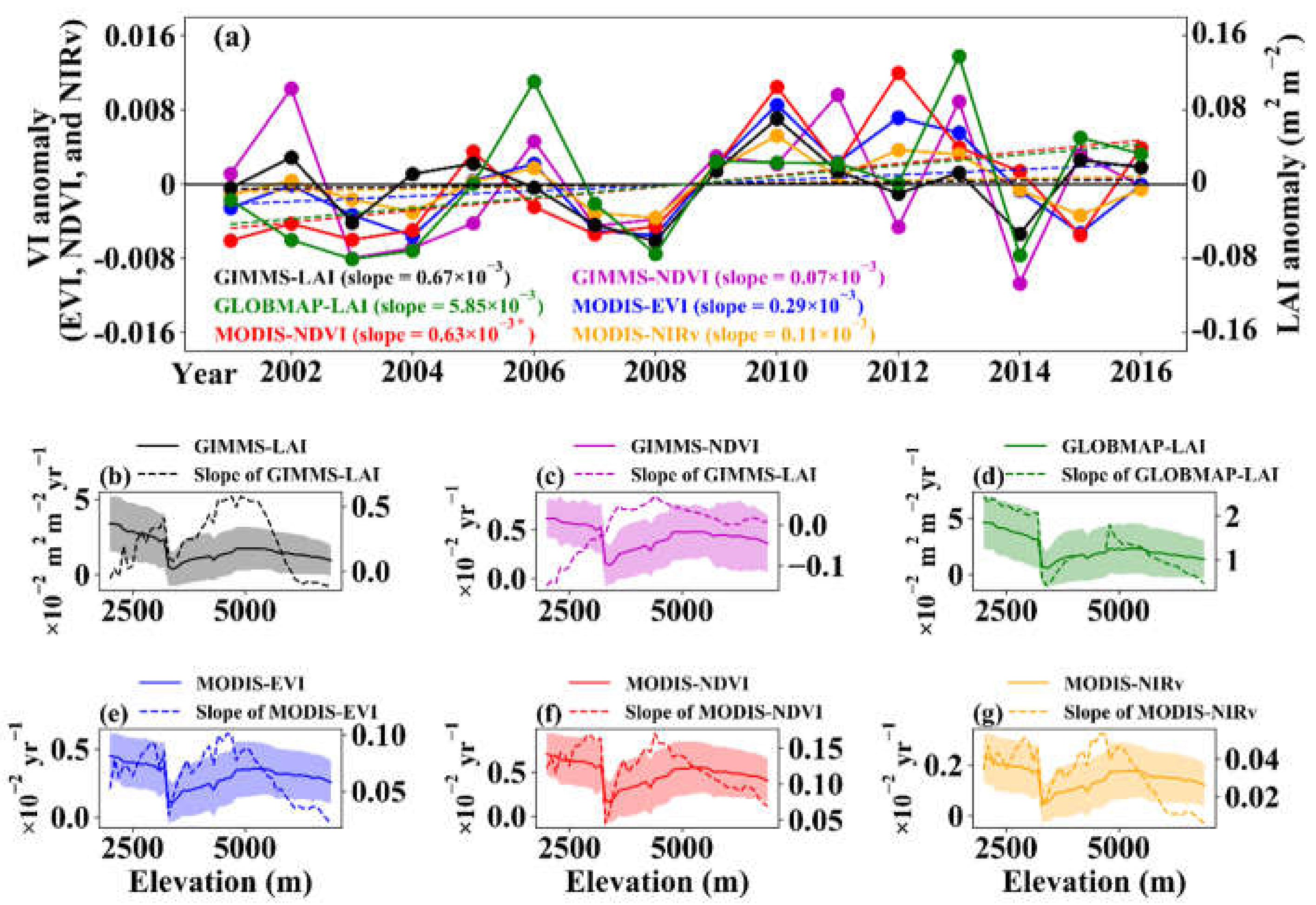
All the VIs exhibited an increasing trend in the QTP from 2001 to 2016 (Figure 5). MODIS NDVI exhibited the highest slope of all VIs (0.67 × 10⁻³/year), followed by MODIS EVI (0.29 × 10⁻³/year) and MODIS NIRv (0.11 × 10⁻³/year), and GIMMS NDVI (0.07 × 10⁻³/year) had the least increase rate. A comparison of the trend of LAIs showed that the slope of GLOBMAP LAI (5.58 × 10⁻³/year) was more than eight times higher than that of GIMMS LAI (0.67 × 10⁻³/year). Overall, only the slope of MODIS NDVI reached the significance level of 0.05. The VIs had a similar elevation distribution to vegetation greenness (Figure 5a). The VIs decreased from low altitude to around 3300 m, and the lowest value of VIs was observed at 3300 m. Since then, the VIs experienced the trends from increase to decrease along elevation gradients (Figure 5b–g). The slope of GIMMS-LAI- and MODIS-derived VIs had similar elevation distribution, that is, it increased first and then dropped quickly to the elevation of around 3300 m. Thereafter, the slope of VIs presented an increasing trend first and then a decreasing trend, whereas such a trend was inconsistent with that of GIMMS NDVI and GLOBMAP LAI.

Figure 5.
Trend of VIs (a) and their elevation distribution (b–g) in the QTP from 2001 to 2016. The dashed straight lines denote the trend lines in (a). The solid and dashed curves denote the mean value and slope of VI in (b–g). Asterisk (*) denotes that the slope is statistically significant at the 0.05 level. The colored shadow region represents one standard deviation.
The spatial patterns of vegetation greenness trend, which were monitored by six kinds of VIs, were not fully consistent with each other from 2001 to 2016 (Figure 6). Overall, the GIMMS-based VIs exhibited an increasing trend in the QTP, and the regions with a significant increasing trend were slightly higher than that with a decreasing trend (9.52% vs. 8.26%). The region showed an increasing trend of GIMMS-based VI in the Northern QTP, while the southern part tended to decrease (Figure 6a,b). These spatial distribution characteristics were obvious in latitude (Figure 6a-2,b-2). By contrast, the overall increasing trend of GIMMS-based VI was more obvious in longitude (Figure 6a-3,b-3). The region with an increasing trend of GLOBMAP LAI was the largest of all VIs, the area of which accounted for 70.21% of the study area and mainly distributed in the Eastern QTP and southern edge of the QTP (Figure 6c-1). The increasing trend was distributed clearly in longitude and latitude (Figure 6c-2,c-3). MODIS-based VI presented an overall increasing trend, as well, from 2001 to 2016. The increasing areas accounted for (66.16 ± 1.59) % of the study area, and (15.72 ± 1.76) % reached significance levels that were far more than those of the significantly decreased area (accounted for 3.01%). The regions with an increasing trend were mainly identified in the Center and Southwestern QTP (Figure 6d-1–f-1). The increase in MODIS-based VIs can be found in high- and low-latitude areas, and the longitude greater than 100° (Figure 6d-2–f-2,d-3–f-3).
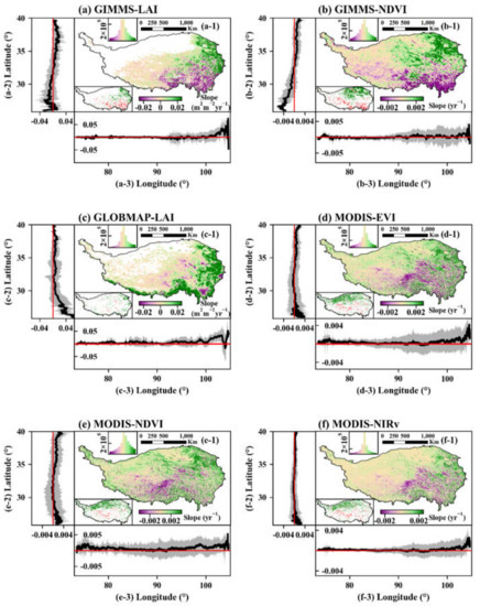
Figure 6.
Spatial pattern of the VIs slope in the QTP from 2001 to 2016 (e-1–f-1). The significance inset of the trend is in the lower-left and the value frequency inset is in the upper-left of each main figure. The subfigures (e-2–f-2) and (e-3–f-3) denote the latitudinal and longitudinal distribution of the VIs slope; the shadow regions represent one standard deviation.
In summary, the consistency of the spatial variation of GIMMS-based VIs was 45.58%; the positive (P) and negative (N) trends were 23.38% and 22.20%, and 15.25% had no data record (Appendix A Figure A1a). By contrast, the overall consistency of MODIS-based VIs was up to 76.73%, and the P and N trends accounted for 54.69% and 22.05% of the study areas (Appendix A Figure A1b). Nevertheless, the whole consistency of the trend of six VIs only occupied 12.62%, and the variation was inconsistent in nearly half of the study area (48.16%) (Appendix A Figure A1c).
3.3. Spatial Patterns and Variations of the VGEG
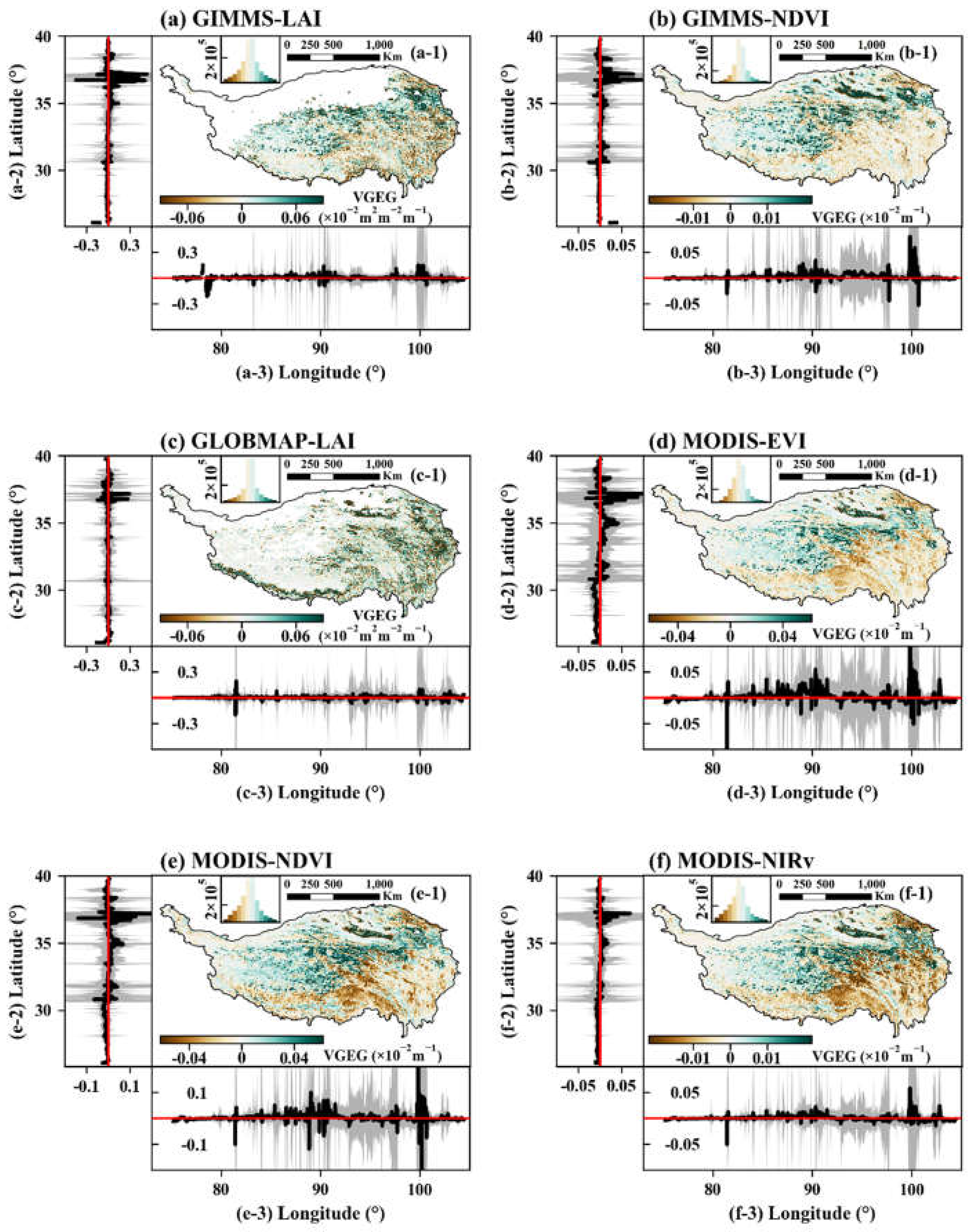
The spatial patterns of VGEG derived from six VIs are shown in Figure 7. The areas of positive VGEG occupied (46.47 ± 3.68) % of the total study area, and (34.37 ± 2.21) % of the region reached a significance level of 0.05. Except for GLOBMAP LAI, the VGEG of other VIs showed obvious spatial distribution characteristics. The areas of positive VGEG are mainly distributed in the Western QTP, as well as in a small part of the Central and Northeastern QTP. By contrast, the region with negative VGEG accounted for (53.53 ± 3.68) %, and the significantly negative region occupied (40.94 ± 6.29) % of the study areas. These areas were identified in the Southeastern QTP.
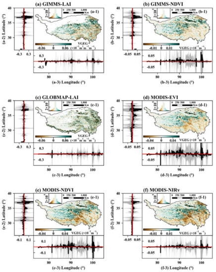
Figure 7.
Spatial pattern of the mean VGEG from 2001 to 2016 (a-1–f-1). The value frequency inset is in the upper-left of each main figure. The subfigures (e-2–f-2) and (e-3–f-3) denote the latitudinal and longitudinal distributions of VGEG; the shadow regions represent one standard deviation.
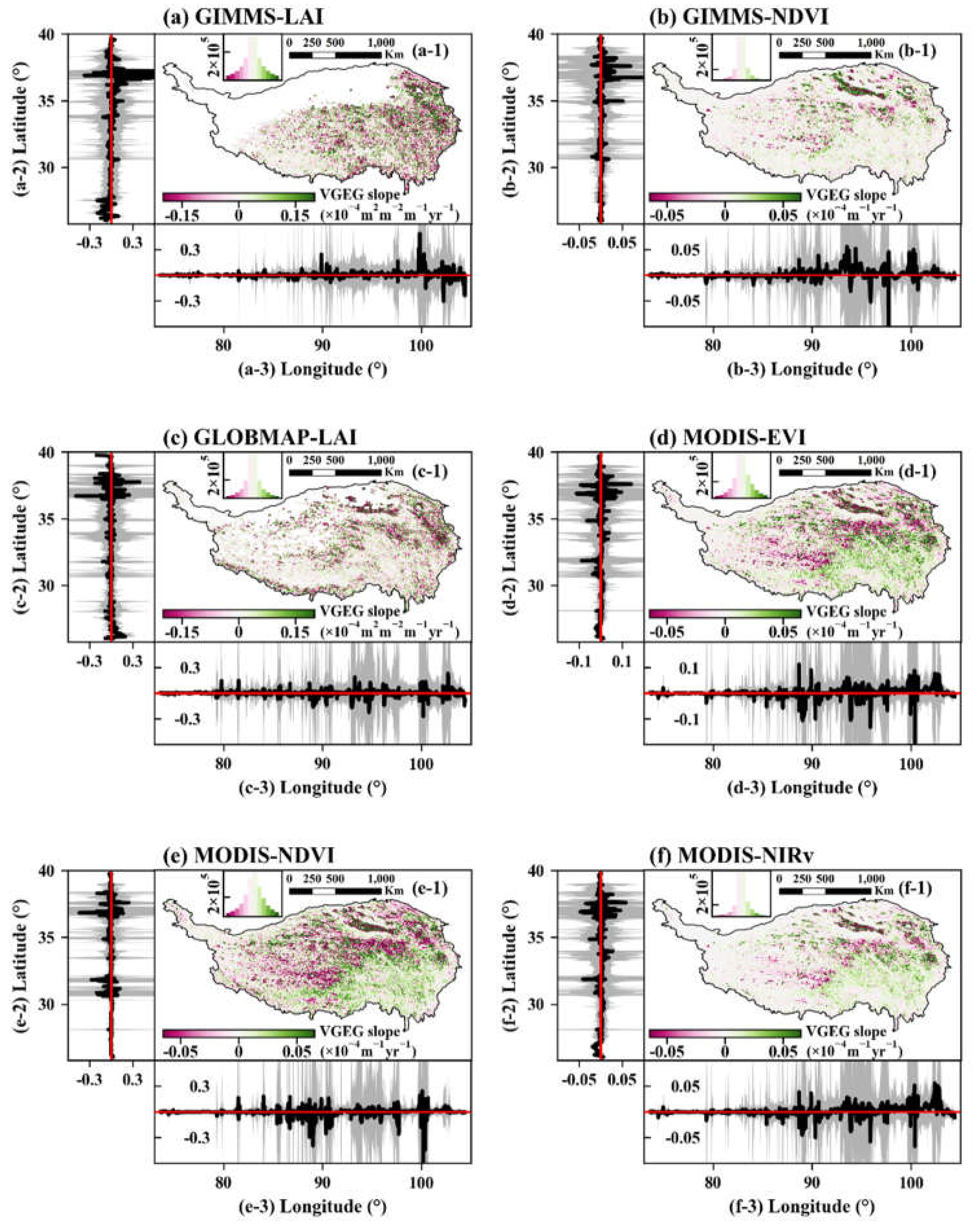
The variations in VGEG based on LAI showed strong spatial heterogeneity during the period (Figure 8a,c), and no obvious characteristics of the spatial distribution were observed. Both LAIs showed that the region with an increasing trend was slightly larger than that with a decreasing trend (51.02% vs. 48.98% by comparing the mean percentage of the two LAIs). By contrast, we found clear spatial distribution patterns of VGEG based on GIMMS NDVI and MODIS-based VI. Specifically, the region with increased VGEG accounted for (53.17 ± 1.28) % of the study area, and it was mainly identified in the Southeastern QTP. By contrast, (46.83 ± 1.28) % of the regions with decreased VGEG were identified in the Northwestern QTP (Figure 8b,d–f).
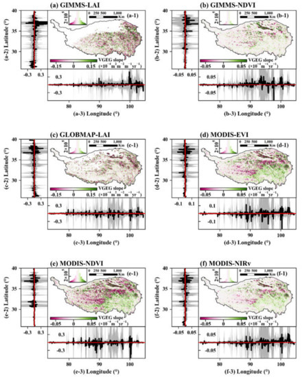
Figure 8.
Spatial pattern of the VGEG variation from 2001 to 2016 (a-1–f-1). The value frequency inset is in the upper-left of each main figure. The subfigures (e-2–f-2) and (e-3–f-3) show the latitudinal and longitudinal distributions of VGEG variation; the shadow regions represent one standard deviation.
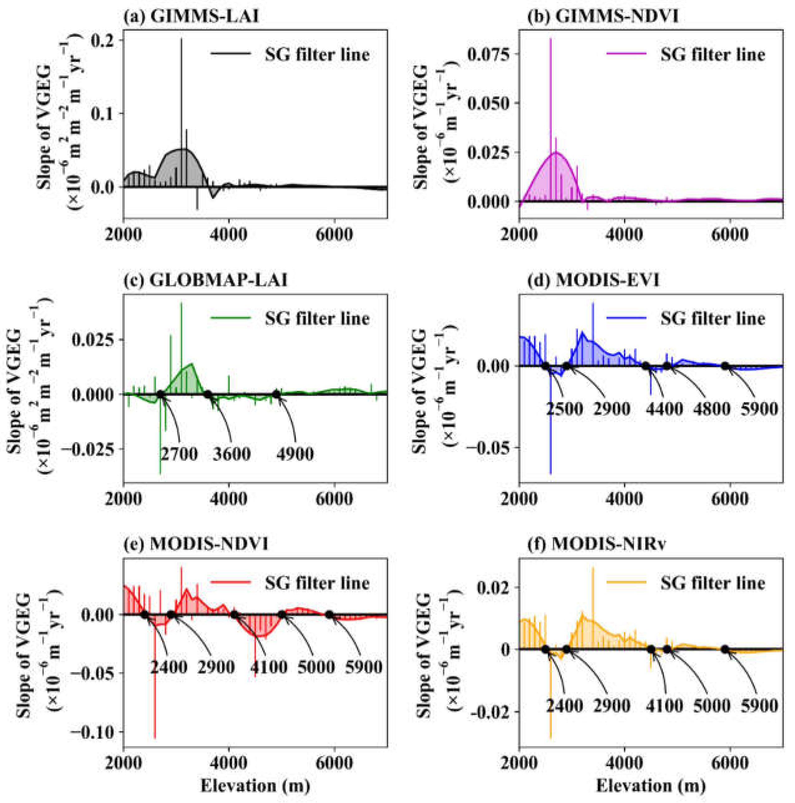
The turning elevation point is marked in Appendix A Figure A2. The low-altitude (lower than 3600 m) region exhibited positive VGEG. By contrast, the high-altitude (greater than 5000 m) region showed negative VGEG. From the altitudes of 3600 to 4100 m and 4100 to 5000 m, negative and positive VGEG alternately appeared, respectively. However, the results of GLOBMAP LAI differed from the other VIs. The variations in VGEG along elevation appeared more complex than its spatial patterns (Appendix A Figure A3). GIMMS-based VIs showed a positive slope of VGEG at the region of lower altitudes (around 3000 m), and insignificant changes were found in other altitude areas. This trend was quite different from that of MODIS-based VI, which represented a positive trend of VGEG at the elevational range of lower than 2500 m, from 2900 to 4100 m, and from 5000 to 5900 m. Negative trends of VGEG were found in 2400 to 2900 m and around 4000 to 5000 m. The results of GLOBMAP LAI were still different from those of the other VIs.
3.4. Effect of Climate on the Zonal Distribution of VI
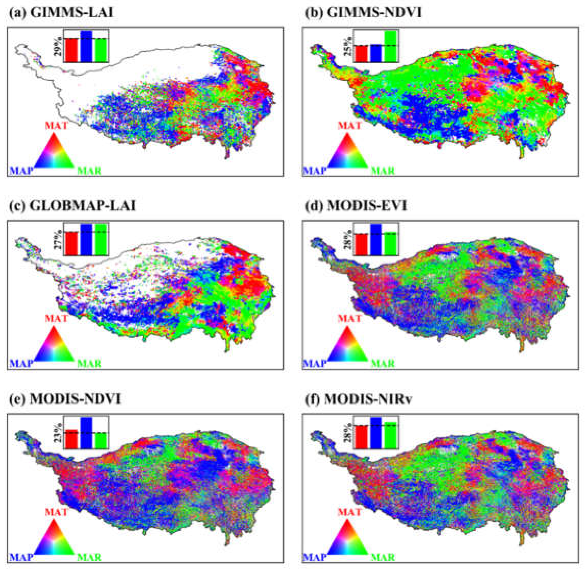
Figure 9 illustrates that, except for the GIMMS NDVI, MAP was the dominating climate factor on the changes in VI in (38.33 ± 6.09) % of the study areas. These areas were mainly found in the southwest and center of the QTP. MAR came second, and the dominated areas of which occupied (33.52 ± 7.34) % of the study areas. MAT had the weakest effect on the variation in VI, and it influenced (28.15 ± 1.65) % of the QTP. These areas were scattered in the western, central, and eastern parts of the QTP. We also analyzed the dynamics of climate in the case of significant variations in the VIs from 2001 to 2016. We used a linear regression method to represent the climate dynamics with significant increasing VIs (Table 2). The correlations between VIs and climate showed that the increase in VI was coupled with increased MAT and MAR, whereas the MAP exhibited a decreasing trend, which indicated that the increase in VIs may be attributed to the increases in MAT and MAR. By contrast, the decrease in VIs corresponded to the increases in MAT and MAR and the decrease in MAP. This finding implied that the increased MAT and decreased MAP are likely to cause an arid environment, which may lead to decreases in VI.
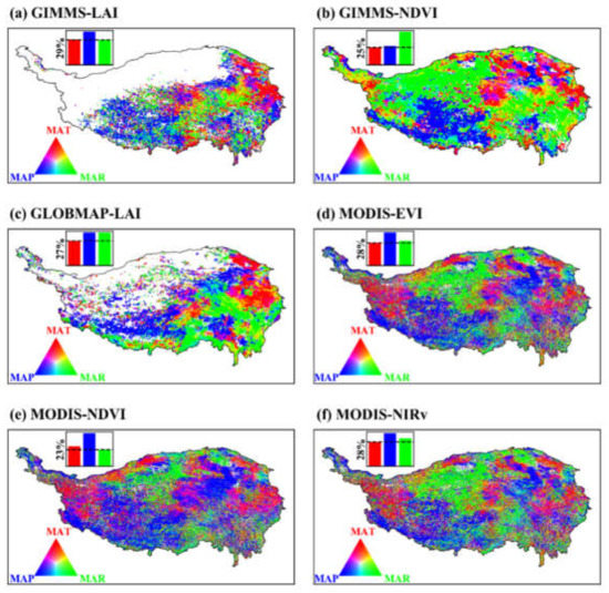
Figure 9.
Spatial pattern of the dominated climate factor for VI inter-annual variability from 2001 to 2016. The regions that tend to red, blue, and green color indicate MAT, MAP, and MAR dominated inter-annual variability of VI. The red, blue, and green bars at the upper-left inset denote the percentage of the areas dominated by MAT, MAP, and MAR, respectively.

Table 2.
Correlation between climate factors and changes in vegetation indices.
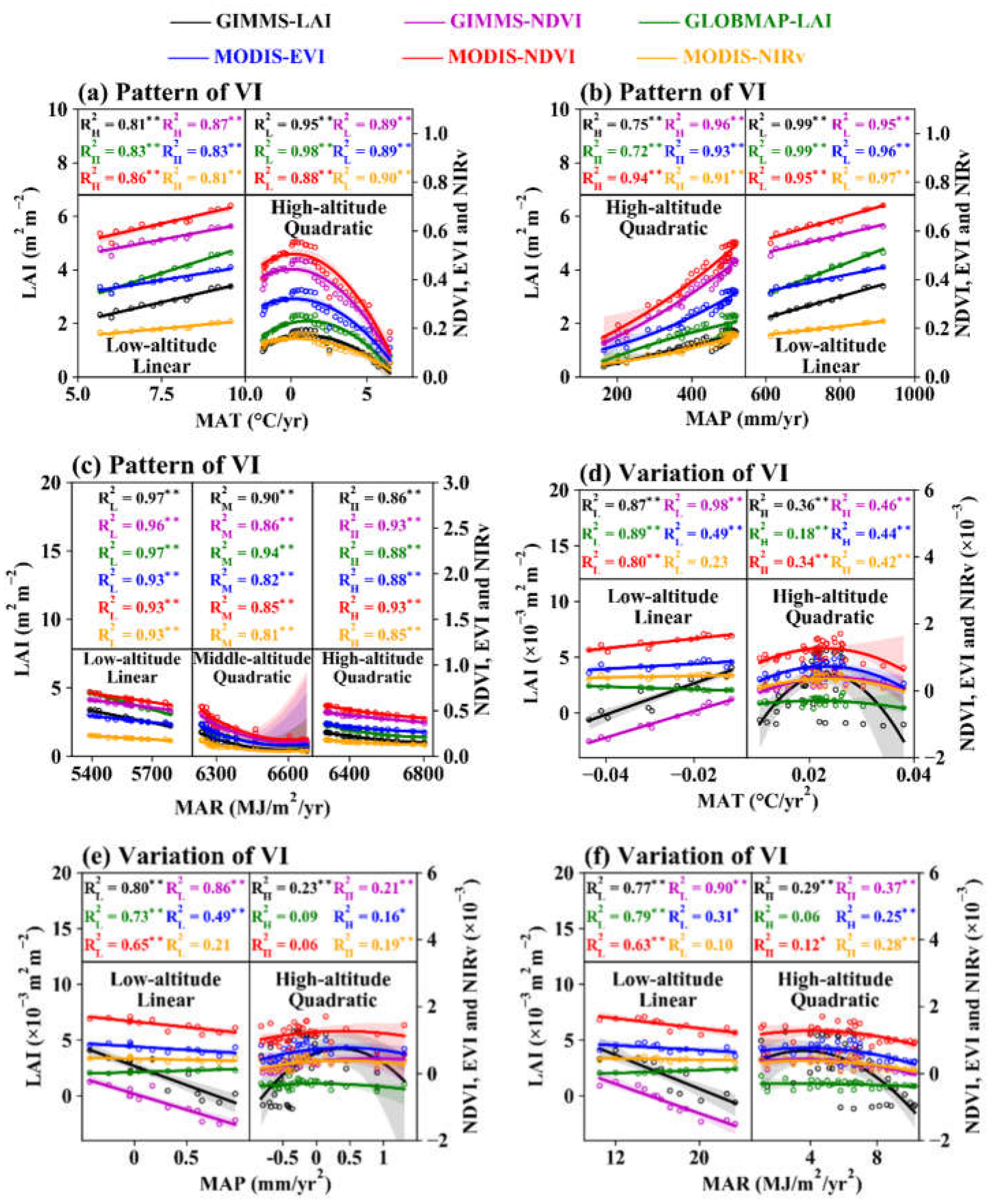
The effect of climate (MAT, MAP, and MAR) on the spatial pattern and variation of VIs along elevational gradients can be expressed as linear and quadratic function at the low (lower than 3300 m) and high altitudes (higher than 3300 m, as annotated in Figure 10). By contrast, the spatial pattern of VI under the influences of MAR in elevation gradients can be divided into low, medium (from 3300 to 5100 m), and high altitudes (higher than 5100 m). At low altitudes, the effect of climate on the elevational distribution of VIs can be expressed as a linear function curve (low altitude in Figure 10a). VI increased with the increases in MAT and MAP (low altitude in Figure 10b). On the contrary, VIs decreased with the increase in MAR at low altitudes (low altitude in Figure 10c). At high altitudes, the effect of climate on the elevational distribution of VIs can be expressed as a quadratic function curve. The VIs stayed stable or slightly increased with the increase in MAT; then VI decreased sharply as the temperature increased (high altitude in Figure 10a). Although VIs decreased with the increase in MAR (high altitude in Figure 10c), the decrease was not as severe as that of MAT. Unlike MAT and MAR, VIs always increased as MAP increased (high altitude in Figure 10b). At middle altitude, the increase in MAR was coupled with decreased VIs (middle altitude in Figure 10c). However, we found large uncertainty of the MAR at higher than 6500 MJ/m2. The R2 of the functions of VIs and climate are shown at the upper part of the figures, all of that reached the significance level of 0.01.
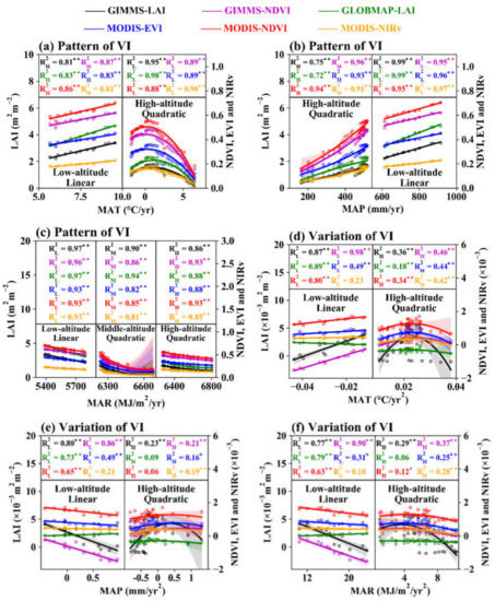
Figure 10.
Effect of climate on the spatial patterns and slopes of VI in elevational gradients. Subfigures illustrate the scatter points and their fitting curves of the correlation between climate and VI spatial patterns (a–c) and slopes (d–f) in elevational gradients. The determination coefficients of VIs and climate are shown at the upper part of each subfigure. The shadow region of each line denotes the 95% confidence level.
MAT exerted a positive effect on the variations in VI along the elevation gradient, which can be described by linear function in low-altitude regions (low altitude in Figure 10d). By contrast, the effects of MAP and MAR were negative on the variations in VI (low altitude in Figure 10e,f). Overall, GIMMS-based VI had a stronger response to the impact of climate. On the contrary, the responses of GLOBMAP LAI to MAT were negative, and positive responses of GLOBMAP LAI to MAP and MAR were observed. On the contrary, the impact of climate on NIRv variations was insignificant. The R2 of these linear functions achieved a significant level of 0.05, except MODIS NIRv. The effect of climate on the variations in VI along the elevation gradient can be described as a quadratic function in high altitudes (high altitude in Figure 10d–f). The R2 of the function between VIs and MAT reached a significance level of 0.01. However, the R2 did not exhibit significance among MODIS NDVI, GLOBMAP LAI, and MAP, as well as GLOBMAP LAI to MAR.
4. Discussion
4.1. Merit and Limitation
The moving window method in this study uses remote-sensing and DEM data to monitor changes in vegetation greenness, along altitude gradients within a moving window extent. It is different from traditional transect survey method, which arranges sample plots on the survey line along the slope of mountain surface to investigate the changes in vegetation characteristics within the plots [44]. The size of the moving window limits the detection in a certain region that enables a comparison between kinds of vegetation greenness under a uniform external environment. Applying the moving window method to analyze remote-sensing data can monitor the changes in vegetation greenness rapidly, effectively, and cheaply on the altitude gradient at the regional or global scale, especially the regions that are difficult to reach by humans. This method has been proven effective by a universal law of nature; that is, the temperature decreases with the increase in altitude (Figure 4b). Notably, the method detects the change of vegetation greenness within the relative height range, and the mutual confirmation with the traditional method requires further research.
Another limitation of the method we concerned is the interpolation of data from large scale to small scale. The resolutions of the climate and GIMMS-based VIs data are 0.1° and ≈0.08°, respectively, which means that we must interpolate the resolution of the two datasets to a finer resolution (0.01°) without losing the information of DEM and MODIS-based VIs data. We know that the variables change slowly in the large-scale extent, representing the circulation characteristics of the large region, while the change processes of small-scale variables are relatively rapid, representing the local climate characteristics. The downscaling interpolation method, that from large-scale to small-scale, cannot increase the effective information of the data. The consequence is that the microclimate characteristics of local regions are likely be ignored, which will make the results highly uncertain, and may even be inconsistent with the facts. We know that the fundamental sources of climate and GIMMS VIs data are meteorological stations and AVHRR sensor. To improve the spatial resolution of the two datasets, the ultimate solution is to establish more meteorological stations and improve the photographing capability of the AVHRR sensor. However, these are difficult to achieve in the short-term. Therefore, we need to carefully judge whether the data resolution matches the spatial extent of the study area to avoid getting incorrect results due to interpolation.
The spatial resolution of VI is strongly affecting the spatial pattern and variation of VGEG [26]. We will inevitably ignore some spatial details at low spatial resolution. However, the higher the spatial resolution, the larger the amount of data and the lower the efficiency of data processing. We recommend choosing high-resolution data as much as possible when the computing power is guaranteed. Moreover, the vegetation types were fixed throughout this study. Therefore, we may have ignored the changes in vegetation types under the influence of climate, especially the diversity of vegetation types on an altitude gradient, which will have a significant impact on NPP, thereby affecting the carbon cycle of the alpine ecosystem. Regardless, whether the vegetation diversity changes along the altitude gradient needs further study.
4.2. Performance of VI and Its Influencing Factors
We found that the performances of the six VIs had large discrepancies in the spatial pattern of inter-annual variation. The overall consistency of the six VIs only accounted for 12.62% of the study areas (Appendix A Figure A1). The photographing capability of satellite sensors is the most important reason. MODIS has 36 spectral bands, and the informative high-quality bands have high calibration accuracy and are ideal for monitoring large-scale changes in the biosphere [36]. By contrast, the AVHRR sensor has only five spectral bands, and it has defects in design and low accuracy in the calibration. Therefore, the quality of GIMMS VIs is lower than that of MODIS VIs [33], although its results may be correct in long-term research.
We found that the vegetation greenness exhibited increasing trends in the QTP from 2001 to 2016, and precipitation was negatively correlated with the increase in vegetation greenness in most areas of the QTP. Therefore, we infer that precipitation is not the dominating climate factor on the increase in vegetation greenness on the QTP, but it is a fundamental environmental factor determines the lower limitation of vegetation growth. By contrast, drought is likely to occur in a water-deficient environment, and it determines the degree of vegetation greenness reduction. Therefore, the combination of temperature and radiation is likely to be the main factor in the increase in vegetation greenness, not solely the increase in temperature. The significant decreases in vegetation greenness probably contribute to the drought. We found that areas with a significant decrease in vegetation greenness were usually accompanied by increased temperature and decreased precipitation. It is worth noting that we assumed that the vegetation greenness is only affected by climate variation. Thus, we inevitably ignored the changes in vegetation greenness caused by human activities, because their complication in the process and spatial identification made us highly uncertain as to their effect on the changes in vegetation greenness [45].
Vegetation greenness is generally negative along the elevation gradient, because the hydrothermal conditions significantly changed with the increase in elevation. A higher altitude corresponds to more limitations of low temperature [46]. However, we found that the increasing rate of temperature was amplified in high-altitude regions (Figure 3b). The warmer climate of the alpine region will promote the growth of alpine grasslands in high-altitude regions under adequate water from the melting of frozen soil and mountain ice and snow [47]. Accelerated warming at high altitudes will result in positive VGEG, which we found to account for more than 34% of the study area. This phenomenon needs to be paid sufficient attention to because its results may not be conducive to the sustainable development of the ecosystem.
4.3. Implications for Alpine Ecosystem
We confirm that the high-altitude area of the QTP has a higher temperature increase rate than the low-altitude area. The increased temperature and radiation are likely to cause the homogenization of vegetation greenness along elevation gradients. The vegetation greenness homogenization can be represented by positive VGEG, the areas of which have reached nearly 34% of the QTP. Such a large area should arouse our attention, especially in the sparsely populated regions that are more likely to be ignored.
Remote-sensing data are essential for accurately simulating vegetation types, a practice that is significant to infer the parameters that affect the physical processes of vegetation and the energy exchange between the atmosphere and the land surface [48]. However, the vegetation types are highly uncertain, especially in high mountainous regions. Because of the height difference, the signal that was originally a ground point is replaced by a high-point signal at the same position, resulting in a displacement of the image point. Moreover, the uncertainty comes from the complexity and diversity of the mechanism of interaction between vegetation and climate factors. However, we found that the elevation distributions of vegetation greenness and its variation are linearly affected by temperature, precipitation, and radiation at low altitudes. By contrast, the effect of climate on vegetation greenness and its variation is nonlinear in high altitudes. If such a relationship is applied to alpine regions on a global scale, it will significantly improve the prediction accuracy of future vegetation types.
The alpine grassland ecosystem is vulnerable to climatic events; small disturbances will cause great changes in the ecosystem [47], such as NPP (net primary productivity). Positive VGEG may imply decreases in the biodiversity of the ecosystem and cause a reduction of the ecosystem resistance and larger proportional loss in NPP to climate extremes [49]. In contrast, the high biodiversity generally provides strong resistance or less productivity loss and stabilizes ecosystem productivity and productivity-dependent ecosystem services, e.g., carbon sequestration [50]. The loss of NPP means a reduction of the photosynthesis capacity of vegetation, coupled with the increase in soil respiration caused by the increase in temperature. The QTP will most likely become a carbon source, and the freezing and thawing of frozen soil and vegetation degradation will accelerate this process [51]. The premise is that we need a reliable terrestrial ecosystem carbon-cycle model to assess carbon dynamics. Unfortunately, there are more models, more processes, and more parameters, but there is no better consistency and fidelity to observations [52]. Therefore, positive VG, as an important feature of ecosystem changes, may help to accurately assess the carbon-cycle process.
5. Conclusions
We can draw the following conclusions from this article. The vegetation was greening in most parts of the QTP from 2001 to 2016; however, we must pay attention to the areas in the Central and Southern QTP that showed vegetation browning. We analyzed climatic factors and conclude that the greening of vegetation is due to the increase in MAT and MAR, while the browning of vegetation is mainly due to drought, that is, the decrease in MAP and increase in MAT.
VIs have a large discrepancy in the trends of vegetation in the QTP from 2001 to 2016. The whole consistency of the trend of six VIs only occupied 12.62%, and the inconsistency of the trends reached nearly half of the study area. The trend of MODIS-based VIs is more consistent than that of GIMMS-based VIs. Therefore, it needs to fully consider the difference between remote-sensing VIs in the simulation of vegetation productivity and evaluate the uncertainty of vegetation productivity caused by such differences.
Notably, we found that the effect of climate on the spatial patterns and variations of vegetation greenness has strong elevational differences: vegetation greenness was linearly correlated with climate at low altitudes and nonlinearly correlated with climate at high altitudes. This conclusion may be helpful for the prediction of vegetation types and their changes in high mountainous regions in the future.
In addition, the regions with significantly positive VGEG were up to (34.37 ± 2.21) % of the QTP, which indicated that the homogenization of the vegetation greenness has already emerged along the elevation gradients in the Western QTP, as well as in a small part of the Central and Northeastern QTP, whereas the decreases in VGEG (46.83% of the QTP) were found in the same regions. This conclusion provides a reference for the monitoring of vegetation changes along the elevation gradients in the QTP, and it is also expected to contribute to environmental management and policy formulation.
Author Contributions
Conceptualization, Z.W.; data curation, Z.W., G.C. and Z.L.; formal analysis, Z.W., G.C. and Z.L.; funding acquisition, X.L., K.Z., G.W. and Z.A.; investigation, Z.W.; methodology, Z.W.; visualization, Z.W.; writing—original draft, Z.W.; writing—review and editing, Z.W., X.L., K.Z. and H.L. All authors have read and agreed to the published version of the manuscript.
Funding
This research was funded by the Open Project of State Key Laboratory of Plateau Ecology and Agriculture, Qinghai University, grant number 2020-ZZ-14, the APC was funded by 2020-ZZ-14; the Open Project of State Key Laboratory of Plateau Ecology and Agriculture, Qinghai University, grant number 2020-ZZ-10; the Open Project of State Key Laboratory of Plateau Ecology and Agriculture, Qinghai University, grant number 2020-ZZ-09; the Open Project of State Key Laboratory of Plateau Ecology and Agriculture, Qinghai University, grant number 2020-ZZ-06; the Basic Research Project of Qinghai Province, China, grant number 2020-ZJ-971Q; the Basic Research Project of Qinghai Province, China, grant number 2020-ZJ-968Q; the trend of grassland and its uncertainty in the Qinghai-Tibet Plateau under global climate change, grant number NKX201918; comparative study on urban heat island effect in the arid and semi-arid areas of China during the past 30 years, grant number NKX201923.
Institutional Review Board Statement
Not applicable.
Informed Consent Statement
Not applicable.
Data Availability Statement
The data presented in this study are openly available in [National Tibetan Plateau Data Center] at [10.11888/AtmosphericPhysics.tpe.249369.file.], reference number [29].
Conflicts of Interest
The authors declare no conflict of interest.
Appendix A
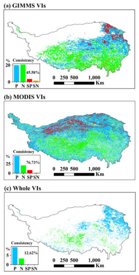
Figure A1.
Consistency of the spatial pattern of the VI variations from 2001 to 2016: (a) represents the consistency of GIMMS Vis, (b) represents the consistency of MODIS Vis, and (c) represents the consistency of all VIs. The percentages of the area of positive (P), negative (N), significantly positive (SP), and significantly negative (SN) consistency are shown in the lower-left inset.


Figure A2.
VGEG distributed in elevational gradients. The black circle denotes the turning elevation, and the solid line denotes the SG filter line.
Figure A2.
VGEG distributed in elevational gradients. The black circle denotes the turning elevation, and the solid line denotes the SG filter line.
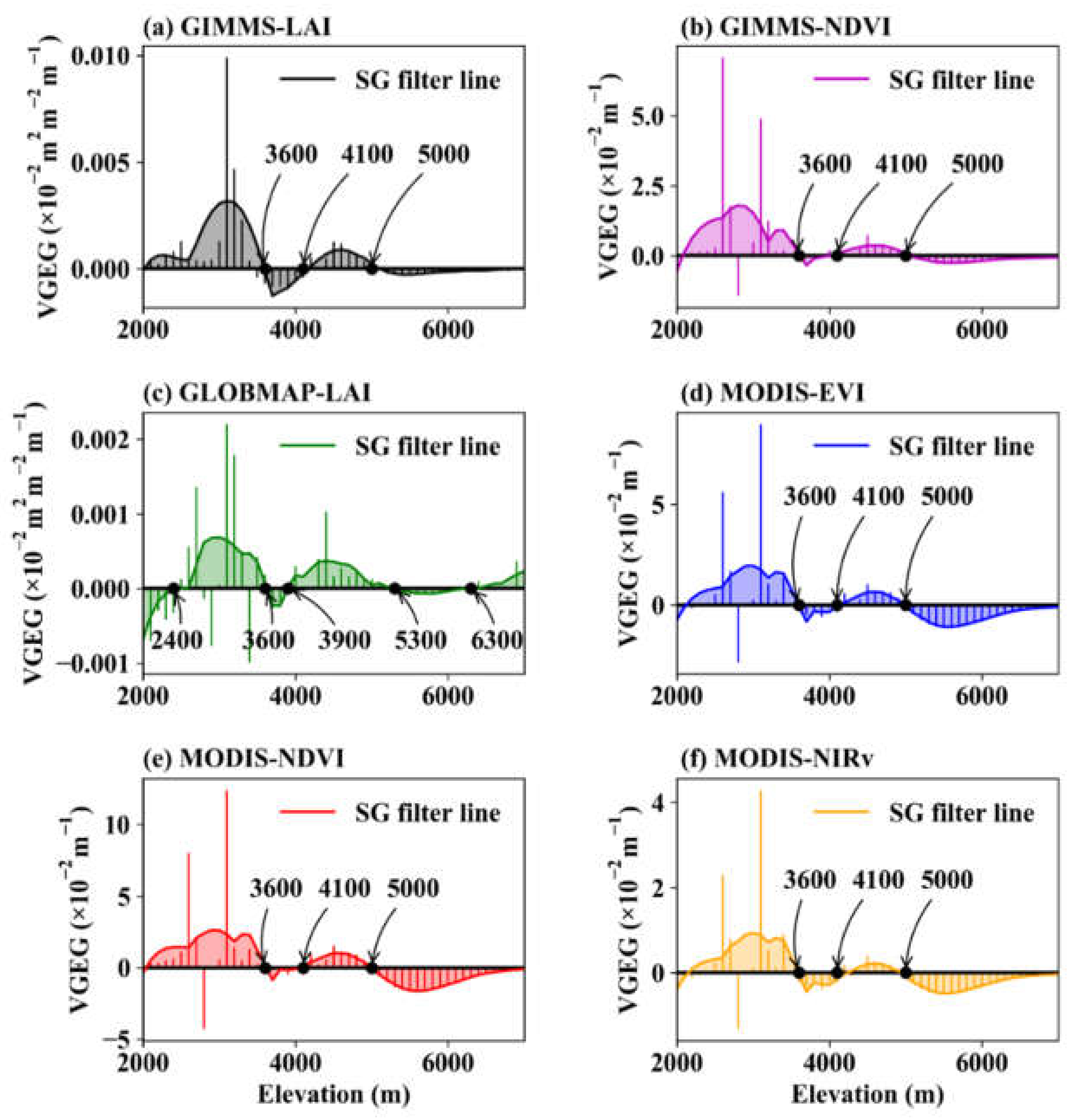

Figure A3.
VGEG variation distributed in elevational gradients. The black circle denotes the turning elevation, and the solid line denotes the SG filter line.
Figure A3.
VGEG variation distributed in elevational gradients. The black circle denotes the turning elevation, and the solid line denotes the SG filter line.
References
- Zhu, Z.; Piao, S.; Yan, T.; Ciais, P.; Bastos, A.; Zhang, X.; Wang, Z. The accelerating land carbon sink of the 2000s may not be driven predominantly by the warming hiatus. Geophys. Res. Lett. 2018, 45, 1402–1409. [Google Scholar] [CrossRef]
- Liu, Y.; Piao, S.; Gasser, T.; Ciais, P.; Yang, H.; Wang, H.; Keenan, T.F.; Huang, M.; Wan, S.; Song, J.; et al. Field-experiment constraints on the enhancement of the terrestrial carbon sink by CO2 fertilization. Nat. Geosci. 2019, 12, 809–814. [Google Scholar] [CrossRef] [Green Version]
- IPCC. Climate Change 2013–The Physical Science Basis: Working Group I Contribution to the Fifth Assessment Report of the Intergovernmental Panel on Climate Change; Cambridge University Press: Cambridge, UK, 2014. [Google Scholar] [CrossRef] [Green Version]
- Rangwala, I.; Miller, J.R. Climate change in mountains: A review of elevation-dependent warming and its possible causes. Clim. Change 2012, 114, 527–547. [Google Scholar] [CrossRef]
- Bertrand, R.; Lenoir, J.; Piedallu, C.; Riofrío-Dillon, G.; de Ruffray, P.; Vidal, C.; Pierrat, J.-C.; Gégout, J.-C. Changes in plant community composition lag behind climate warming in lowland forests. Nature 2011, 479, 517–520. [Google Scholar] [CrossRef]
- Alward, R.D.; Detling, J.K.; Milchunas, D.G. Grassland Vegetation Changes and Nocturnal Global Warming. Science 1999, 283, 229. [Google Scholar] [CrossRef] [PubMed] [Green Version]
- Li, H.; Jiang, J.; Chen, B.; Li, Y.; Xu, Y.; Shen, W. Pattern of NDVI-based vegetation greening along an altitudinal gradient in the eastern Himalayas and its response to global warming. Environ. Monit. Assess. 2016, 188, 186. [Google Scholar] [CrossRef]
- Pepin, N.; Bradley, R.; Diaz, H.; Baraër, M.; Caceres, E.; Forsythe, N.; Fowler, H.; Greenwood, G.; Hashmi, M.; Liu, X. Elevation-dependent warming in mountain regions of the world. Nat. Clim. Change 2015, 5, 424–430. [Google Scholar] [CrossRef] [Green Version]
- Gao, M.; Piao, S.; Chen, A.; Yang, H.; Liu, Q.; Fu, Y.H.; Janssens, I.A. Divergent changes in the elevational gradient of vegetation activities over the last 30 years. Nat. Commun. 2019, 10, 2970. [Google Scholar] [CrossRef] [PubMed]
- Pearson, R.G.; Phillips, S.J.; Loranty, M.M.; Beck, P.S.; Damoulas, T.; Knight, S.J.; Goetz, S.J. Shifts in Arctic vegetation and associated feedbacks under climate change. Nat Clim. Change 2013, 3, 673–677. [Google Scholar] [CrossRef]
- Shen, M.; Zhang, G.; Cong, N.; Wang, S.; Kong, W.; Piao, S. Increasing altitudinal gradient of spring vegetation phenology during the last decade on the Qinghai–Tibetan Plateau. Agr For. Meteorol. 2014, 189, 71–80. [Google Scholar] [CrossRef]
- Qin, J.; Yang, K.; Liang, S.; Guo, X. The altitudinal dependence of recent rapid warming over the Tibetan Plateau. Clim. Change 2009, 97, 321–327. [Google Scholar] [CrossRef]
- Qiu, J. The third pole. Nature 2008, 454, 393–396. [Google Scholar] [CrossRef] [Green Version]
- Piao, S.; Tan, K.; Nan, H.; Ciais, P.; Fang, J.; Wang, T.; Vuichard, N.; Zhu, B. Impacts of climate and CO2 changes on the vegetation growth and carbon balance of Qinghai-Tibetan grasslands over the past five decades. Glob. Planet. Change 2012, 98, 73–80. [Google Scholar] [CrossRef]
- Zhao, L.; Li, Y.; Xu, S.; Zhou, H.; Gu, S.; Yu, G.; Zhao, X. Diurnal, seasonal and annual variation in net ecosystem CO2 exchange of an alpine shrubland on Qinghai-Tibetan plateau. Glob. Change Biol. 2006, 12, 1940–1953. [Google Scholar] [CrossRef]
- Kato, T.; Tang, Y.; Gu, S.; Cui, X.; Hirota, M.; Du, M.; Li, Y.; Zhao, X.; Oikawa, T. Carbon dioxide exchange between the atmosphere and an alpine meadow ecosystem on the Qinghai–Tibetan Plateau, China. Agr. For. Meteorol. 2004, 124, 121–134. [Google Scholar] [CrossRef]
- Piao, S.L.; Fang, J.Y.; He, J.S. Variations in vegetation net primary production in the Qinghai-Xizang Plateau, China, from 1982 to 1999. Clim. Change 2006, 74, 253–267. [Google Scholar] [CrossRef]
- Wang, X.; Chen, D. Interannual variability of GNDVI and its relationship with altitudinal in the Three-River Headwater Region. Ecol. Environ. Sci. 2018, 27, 1411–1416. [Google Scholar] [CrossRef]
- Li, L.; Zhang, Y.; Wu, J.; Li, S.; Zhang, B.; Zu, J.; Zhang, H.; Ding, M.; Paudel, B. Increasing sensitivity of alpine grasslands to climate variability along an elevational gradient on the Qinghai-Tibet Plateau. Sci. Total Environ. 2019, 678, 21–29. [Google Scholar] [CrossRef]
- Meng, X.; Gao, X.; Li, S.; Lei, J. Spatial and temporal characteristics of vegetation NDVI changes and the driving forces in Mongolia during 1982–2015. Remote Sens. 2020, 12, 603. [Google Scholar] [CrossRef] [Green Version]
- Pan, N.; Feng, X.; Fu, B.; Wang, S.; Ji, F.; Pan, S. Increasing global vegetation browning hidden in overall vegetation greening: Insights from time-varying trends. Remote Sens. Environ. 2018, 214, 59–72. [Google Scholar] [CrossRef]
- Liu, Z.; Wimberly, M.C.; Dwomoh, F.K. Vegetation Dynamics in the Upper Guinean Forest Region of West Africa from 2001 to 2015. Remote Sens. 2016, 9, 5. [Google Scholar] [CrossRef] [Green Version]
- Zhu, Z.; Piao, S.; Myneni, R.B.; Huang, M.; Zeng, Z.; Canadell, J.G.; Ciais, P.; Sitch, S.; Friedlingstein, P.; Arneth, A. Greening of the Earth and its drivers. Nat. Clim. Change 2016, 6, 791–795. [Google Scholar] [CrossRef]
- Chen, C.; Park, T.; Wang, X.; Piao, S.; Xu, B.; Chaturvedi, R.K.; Fuchs, R.; Brovkin, V.; Ciais, P.; Fensholt, R.; et al. China and India lead in greening of the world through land-use management. Nat. Sustain. 2019, 2, 122–129. [Google Scholar] [CrossRef]
- Yuan, W.; Zheng, Y.; Piao, S.; Ciais, P.; Lombardozzi, D.; Wang, Y.; Ryu, Y.; Chen, G.; Dong, W.; Hu, Z.J.S.A. Increased atmospheric vapor pressure deficit reduces global vegetation growth. Sci. Adv. 2019, 5, eaax1396. [Google Scholar] [CrossRef] [Green Version]
- Wang, Z.; Liu, X.; Wang, H.; Zheng, K.; Li, H.; Wang, G.; An, Z. Monitoring Vegetation Greenness in Response to Climate Variation along the Elevation Gradient in the Three-River Source Region of China. ISPRS Int. J. Geo-Inf. 2021, 10, 193. [Google Scholar] [CrossRef]
- Foggin, J.M. Depopulating the Tibetan Grasslands. Mt. Res. Dev. 2008, 28, 26–31. [Google Scholar] [CrossRef] [Green Version]
- Zhang, X. Vegetation of China and Its Geographic Pattern: Illustration of the Vegetation Map of the People's Republic of China (1:1000 000); Geological Publishing House: Beijing, China, 2007. [Google Scholar]
- He, J.; Yang, K.; Tang, W.; Lu, H.; Qin, J.; Chen, Y.; Li, X. The first high-resolution meteorological forcing dataset for land process studies over China. Sci. Data 2020, 7, 25. [Google Scholar] [CrossRef] [PubMed] [Green Version]
- Piao, S.; Cui, M.; Chen, A.; Wang, X.; Ciais, P.; Liu, J.; Tang, Y. Altitude and temperature dependence of change in the spring vegetation green-up date from 1982 to 2006 in the Qinghai-Xizang Plateau. Agr. For. Meteorol. 2011, 151, 1599–1608. [Google Scholar] [CrossRef]
- Zheng, D. The system of physico-geographical regions of the Qinghai-Xizang (Tibet) Plateau. Sci. China 1996, 4, 410–417. [Google Scholar]
- Tucker, C.J.; Fung, I.Y.; Keeling, C.D.; Gammon, R.H. Relationship between atmospheric CO2 variations and a satellite-derived vegetation index. Nature 1986, 319, 195–199. [Google Scholar] [CrossRef]
- Pinzon, J.; Tucker, C. A Non-Stationary 1981–2012 AVHRR NDVI3g Time Series. Remote Sens. 2014, 6, 6929. [Google Scholar] [CrossRef] [Green Version]
- Zhu, Z.; Bi, J.; Pan, Y.; Ganguly, S.; Anav, A.; Xu, L.; Samanta, A.; Piao, S.; Nemani, R.R.; Myneni, R.B. Global data sets of vegetation leaf area index (LAI) 3g and Fraction of Photosynthetically Active Radiation (FPAR) 3g derived from Global Inventory Modeling and Mapping Studies (GIMMS) Normalized Difference Vegetation Index (NDVI3g) for the period 1981 to 2011. Remote Sens. 2013, 5, 927–948. [Google Scholar] [CrossRef] [Green Version]
- Liu, Y.; Liu, R.; Chen, J.M. Retrospective retrieval of long-term consistent global leaf area index (1981–2011) from combined AVHRR and MODIS data. J. Geophys. Res. Biogeosciences 2012, 117, G04003. [Google Scholar] [CrossRef]
- Huete, A.; Didan, K.; Miura, T.; Rodriguez, E.P.; Gao, X.; Ferreira, L.G. Overview of the radiometric and biophysical performance of the MODIS vegetation indices. Remote Sens. Environ. 2002, 83, 195–213. [Google Scholar] [CrossRef]
- Badgley, G.; Field, C.B.; Berry, J.A. Canopy near-infrared reflectance and terrestrial photosynthesis. Sci. Adv. 2017, 3, e1602244. [Google Scholar] [CrossRef] [PubMed] [Green Version]
- Holben, B.N. Characteristics of maximum-value composite images from temporal AVHRR data. Int. J. Remote Sens. 1986, 7, 1417–1434. [Google Scholar] [CrossRef]
- Gang, C.; Wang, Z.; Chen, Y.; Yang, Y.; Li, J.; Cheng, J.; Qi, J.; Odeh, I. Drought-induced Dynamics of Carbon and Water Use Efficiency of Global Grasslands from 2000 to 2011. Ecol. Indic. 2016, 67, 788–797. [Google Scholar] [CrossRef]
- Zhang, Y.; Wang, Q.; Wang, Z.; Yang, Y.; Li, J. Impact of human activities and climate change on the grassland dynamics under different regime policies in the Mongolian Plateau. Sci. Total Environ. 2020, 698, 134304. [Google Scholar] [CrossRef] [PubMed]
- Zhang, Y.; Zhang, C.; Wang, Z.; Chen, Y.; Gang, C.; An, R.; Li, J. Vegetation dynamics and its driving forces from climate change and human activities in the Three-River Source Region, China from 1982 to 2012. Sci. Total Environ. 2016, 563, 210–220. [Google Scholar] [CrossRef]
- Chen, J.; Yan, F.; Lu, Q. Spatiotemporal Variation of Vegetation on the Qinghai–Tibet Plateau and the Influence of Climatic Factors and Human Activities on Vegetation Trend (2000–2019). Remote Sens. 2020, 12, 3150. [Google Scholar] [CrossRef]
- Pearson, E.S. The Test of Significance for the Correlation Coefficient. J. Am. Stat. Assoc. 1931, 26, 128–134. [Google Scholar] [CrossRef]
- Meng, F.; Cui, S.; Wang, S.; Duan, J.; Jiang, L.; Zhang, Z.; Luo, C.; Wang, Q.; Zhou, Y.; Li, X. Changes in phenological sequences of alpine communities across a natural elevation gradient. Agr. For. Meteorol. 2016, 224, 11–16. [Google Scholar] [CrossRef] [Green Version]
- Wang, Z.; Zhang, Y.; Yang, Y.; Zhou, W.; Gang, C.; Zhang, Y.; Li, J.; An, R.; Wang, K.; Odeh, I.; et al. Quantitative assess the driving forces on the grassland degradation in the Qinghai–Tibet Plateau, in China. Ecol. Inform. 2016, 33, 32–44. [Google Scholar] [CrossRef]
- Körner, C. The use of ‘altitude’ in ecological research. Trends Ecol. Evol. 2007, 22, 569–574. [Google Scholar] [CrossRef]
- Wang, Z.; Chang, J.; Peng, S.; Piao, S.; Ciais, P.; Betts, R. Changes in productivity and carbon storage of grasslands in China under future global warming scenarios of 1.5 °C and 2 °C. J. Plant Ecol. 2019, 12, 804–814. [Google Scholar] [CrossRef]
- Strahler, A. Modis Land Cover Product Algorithm Theoretical Basis Document (ATBD) Version 5.0. 1999. Available online: http://modis.gsfc.nasa.gov/data/atbd/atbd_mod12.pdf (accessed on 12 September 2021).
- Isbell, F.; Craven, D.; Connolly, J.; Loreau, M.; Schmid, B.; Beierkuhnlein, C.; Bezemer, T.M.; Bonin, C.; Bruelheide, H.; de Luca, E.; et al. Biodiversity increases the resistance of ecosystem productivity to climate extremes. Nature 2015, 526, 574–577. [Google Scholar] [CrossRef] [PubMed]
- Lange, M.; Eisenhauer, N.; Sierra, C.A.; Bessler, H.; Engels, C.; Griffiths, R.I.; Mellado-Vázquez, P.G.; Malik, A.A.; Roy, J.; Scheu, S. Plant diversity increases soil microbial activity and soil carbon storage. Nat. Commun. 2015, 6, 6707. [Google Scholar] [CrossRef] [PubMed]
- Wang, T.; Yang, D.; Yang, Y.; Piao, S.; Li, X.; Cheng, G.; Fu, B. Permafrost thawing puts the frozen carbon at risk over the Tibetan Plateau. Sci. Adv. 2020, 6, eaaz3513. [Google Scholar] [CrossRef]
- Prentice, I.C.; Liang, X.; Medlyn, B.E.; Wang, Y.P. Reliable, robust and realistic: The three r's of next-generation land-surface modelling. Atmos. Chem. Phys. 2015, 15, 5987–6005. [Google Scholar] [CrossRef] [Green Version]
Publisher’s Note: MDPI stays neutral with regard to jurisdictional claims in published maps and institutional affiliations. |
© 2021 by the authors. Licensee MDPI, Basel, Switzerland. This article is an open access article distributed under the terms and conditions of the Creative Commons Attribution (CC BY) license (https://creativecommons.org/licenses/by/4.0/).


