Abstract
RCS reconstruction is an important way to reduce the measurement time in anechoic chambers and expand the radar original data, which can solve the problems of data scarcity and a high measurement cost. The greedy pursuit, convex relaxation, and sparse Bayesian learning-based sparse recovery methods can be used for parameter estimation. However, these sparse recovery methods either have problems in solving accuracy or selecting auxiliary parameters, or need to determine the probability distribution of noise in advance. To solve these problems, a non-parametric Sparse Iterative Covariance Estimation (SPICE) algorithm with global convergence property based on the sparse Geometrical Theory of Diffraction (GTD) model (GTD–SPICE) is employed for the first time for RCS reconstruction. Furthermore, an improved coarse-to-fine two-stage SPICE method (DE–GTD–SPICE) based on the Damped Exponential (DE) model and the GTD model (DE–GTD) is proposed to reduce the computational cost. Experimental results show that both the GTD–SPICE method and the DE–GTD–SPICE method are reliable and effective for RCS reconstruction. Specifically, the DE–GTD–SPICE method has a shorter computational time.
1. Introduction
Radar cross section (RCS) is a physical quantity to measure the scattering ability of radar targets [1]. It is closely related to the physical properties of the target (such as shape, volume, surface material, etc.) and state properties (such as position, speed, attitude, etc.). After the processing of RCS data, the scattering distribution and status information of targets can be obtained, such as radar SAR/ISAR imaging [2,3] and radar automatic target recognition [4,5,6], etc. In general, the main methods to obtain RCS data include electromagnetic calculation in software, a scattering measurement in anechoic chambers, and a scattering measurement in an open area test site (OATS), under far-field conditions. The electromagnetic simulation method has the advantages of a low cost and a short period of time, but the authenticity of the RCS data cannot be guaranteed. The RCS data measured in an OATS has the highest reliability, yet the measurement is extremely expensive and the confidentiality is poor. In contrast, the RCS data measured in anechoic chambers has a lower cost than in an OATS, and has higher data authenticity than by electromagnetic calculation in software.
In the early stages, the continuous wave (CW) is utilized for scattering measurements in anechoic chambers [7]. Since the CW radar transmits radio wave signals at a particular frequency, and there is no range gate, the RCS data measured by this waveform can be easily susceptible to clutter and cannot be used to determine the range of target. To overcome these problems, the ultra-wideband (UWB) techniques are used [8,9,10]. The linear frequency modulated (LFM) radar can acquire the RCS data of an attitude of the target at a time after a matched filtering and an inverse fast Fourier transform (IFFT). In contrast, the stepped frequency radar works by transmitting stepped frequency signals in sequence. Each measurement can only obtain RCS data (including the amplitude and phase), which has higher accuracy than the LFM radar. Since the stepped frequency radar measures RCS data frequency by frequency, it has a long measurement time. In recent years, for full characteristic information regarding the target, the measurement of bistatic RCS has also been used in anechoic chambers [11,12], which has greatly enriched the original RCS data. The stepped frequency RCS measurement is a very classic RCS measurement method in anechoic chambers. Compared with other methods, it has the advantages of higher frequency stability, more accurate measurement results, and a larger dynamic range.
In fact, the stepped frequency radar in anechoic chambers does not need to measure all RCS data frequency by frequency over the bandwidth, with the help of RCS reconstruction. Only a part of them needs to be measured in anechoic chambers, which can significantly reduce the measurement time. After accurate RCS reconstruction, the reconstructed RCS data can be very close to the real RCS data, so that the stepped frequency radar virtually measures all RCS data over the entire bandwidth. In general, the RCS reconstruction consists of three main steps. The first step is to adopt a reasonable scattering model. At high frequencies, the backscattering fields of radar targets can be approximated as the sum of scattering fields from individual scattering centers (SCs) [13,14]. These SCs can be described by different scattering models. The Damped Exponential (DE) model can represent the point scattering center [15], and it has been widely used in high resolution radar imaging [16,17,18]. However, the DE model can only represent the scattering location and scattering intensity. In contrast, the Geometrical Theory of Diffraction (GTD) is closer to an electromagnetic scattering mechanism, and can precisely represent complex diffraction scattering behaviors [13,14,19]. Thus, it can precisely reflect geometric structures of radar targets, and can accurately represent RCS data in large relative bandwidths.
The second step is to estimate the scattering parameter. There are three main ways to obtain the scattering parameter estimation (SPE) of the GTD model. As a kind of general method, the modern spectrum estimation technique has been applied at an earlier time [20,21,22]. However, this kind of method cannot deal with non-uniform and incomplete data. Probabilistic-based Maximum Likelihood Estimation (MLE) is another kind of effective method for SPE [23], in addition to the Approximate Maximum Likelihood (AML) algorithm, the Coherent Particle Swarm Optimization (CPSO) algorithm [24], the RELAX algorithm [25], etc. However, this kind of method needs huge computing resources, and its solutions are sensitive to the initial value of the iteration. Due to the fact that SCs are sparsely distributed in radar targets at high frequency, the sparse recovery methods can be utilized for SPE [26,27,28,29]. These methods can be subdivided into three major classes: the greedy pursuit method [30], the convex relaxation method [31], and the sparse Bayesian learning method [32]. The greedy pursuit method extracts a non-zero component in each iteration, and provides a fast solution with a low computational cost. Yet, the convergence is not guaranteed. The convex relaxation method has good performance in sparse recovery and has been widely applied in biomedical imaging and radar imaging. However, the performance of this method is sensitive to the selection of the auxiliary parameter. The sparse Bayesian learning method can avoid the selection of auxiliary parameters and can achieve high precision recovery, whereas it needs to assume the noise s probability distribution in advance. In practice, the assumption of the noise s probability distribution is sometimes inappropriate. The last step is to calculate the RCS data. Theoretically, with the adopted scattering model and the estimated scattering parameter, the RCS data at any frequency in the bandwidth can be reconstructed. In this paper, we only consider the reconstruction at stepped frequencies.
To reduce the measurement time of the stepped frequency radar in anechoic chambers, a random frequency-hopping pattern is utilized in this paper. In this pattern, the stepped frequency radar only randomly measures a part of stepped frequencies in the bandwidth. We call this measured pattern the frequency-hopping pattern, and call these measured RCS data the frequency-hopping RCS sequence. Aiming at accurate RCS reconstruction, a non-parametric SPICE algorithm [33,34] combined with the sparse GTD model (referred to as the GTD–SPICE method) is proposed, which enjoys global convergence properties. Firstly, a sparse GTD model is utilized to model the frequency-hopping RCS sequence. Secondly, the SPICE algorithm based on the covariance matrix fitting (CMF) criterion is employed for SPE. Then, the frequency-hopping RCS sequence can be reconstructed. However, this method is intensively computational due to the large dictionary matrix of the sparse GTD model. Furthermore, to reduce the computational cost, an improved coarse-to-fine two-stage SPICE method based on the Damped Exponential (DE) model and the GTD model (referred to as the DE–GTD–SPICE method) is proposed. In the coarse estimation stage, the sparse DE model with fewer scattering parameter is used to coarsely extract the scattering location to determine the candidate distribution intervals of SCs. In the fine estimation stage, a refined sparse GTD dictionary matrix is formed according to the obtained candidate distribution intervals. Then, the SPE is solved by the SPICE algorithm, and the frequency-hopping RCS sequence is reconstructed. Experimental results show that both the proposed GTD–SPICE method and the improved DE–GTD–SPICE method are reliable and effective for RCS reconstruction. In particular, the DE–GTD–SPICE method has a shorter computational time.
The rest of this paper is organized as follows. In Section 2, the GTD model and its sparse representation for random frequency-hopping sequence are introduced. Section 3 proposes the GTD–SPICE method and the improved DE–GTD–SPICE method. Section 4 analyzes the computational complexity of the two methods in detail. Section 5 discusses experiments, and Section 6 draws the conclusion.
2. Signal Model and Sparse Representations
A frequency-hopping pattern is a subsampling working mode of the stepped frequency scattering measurement, which reduces the number of measurements in anechoic chambers. It can also be considered as a sparse stepped frequency pattern. In this section, the GTD model and its sparse representation of random frequency-hopping sequence are introduced.
2.1. GTD Model
According to the GTD model, the backscattered data from radar targets can be well approximated by the vector summation of several equivalent SCs along the line of sight (LOS) [13]. The GTD model can be expressed as:
where , , and represent the backscattered data from radar targets, the number of SCs, and the propagation speed of the radar signal, respectively. Assume that is the initial frequency, and denotes scattering location, the scattering intensity, and scattering type of the scattering center, respectively. The scattering type can be as , which represents different scattering geometrics of radar targets [13].
A general coherent stepped scattering measurement system emits coherent point frequency signals in sequence. Since the frequency of the emitted signal increases uniformly by (frequency-sweeping interval), it is like a process of frequency-sweeping measurement in the entire bandwidth. Then, (1) can be discretely reformulated as:
where , for , represents the backscattered value at the n-th stepped frequency point, and is the frequency of the n-th stepped frequency point. Accordingly, the bandwidth is , the maximum unambiguous distance is , and the normal range resolution is .
Consider a special case where is identically zero. In this case, (2) can be simplified as:
where (3) degenerates to the DE model. Thus, when using the DE model to represent the complex scattering phenomenon, there might be model mismatches with respect to scattering type.
Instead of transmitting N point frequency signals in (2), the frequency-hopping pattern only transmits Q point frequency signals (). Let be the index vector denoting the emitted signals in the frequency-hopping pattern. Thus, is a subset consisting of Q elements, i.e., .Let us define the frequency-hopping ratio (FHR) as follows:
where is the ratio of the number of the reduced measured frequency points by the frequency-hopping pattern, to the number of measured frequency points by the traditional frequency-sweeping pattern in anechoic chambers. It denotes the degree of compression of the original RCS data.
2.2. Sparse GTD Model
To give the sparse GTD model, a uniform discretization in is carried out [35]. Based on the achieved , a more precise one-dimensional uniform grid is conducted. Then, the is subdivided into L range cells, leading to a finer sampling range interval . Accordingly, the total number of range cells becomes in .
Assume that the range resolution after grid division is high enough that all SCs can be approximated on the grids. In this case, (2) can be further reformulated as:
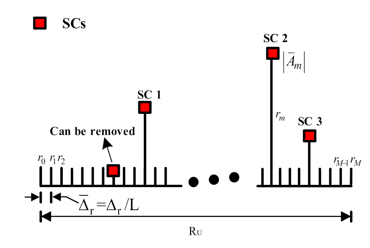
where is the backscattered value in transmitted signal, is the index of the grid point, and , and refer to the scattering intensity, scattering location, and scattering type on the grid point, respectively. When the modulus of i.e., is small enough, it can be assumed that there is no scattering center on the grid. The diagram of the distribution of SCs is shown in Figure 1.
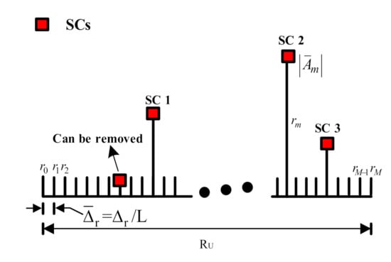
Figure 1.
Diagram of the distribution of SCs.
According to and , (5) can be further reformulated as:
Similar to (3), when is identically zero,(6) can be simplified as:
(7) is an expression of the well-known Discrete Fourier Transform (DFT), and it can be used to compose the sparse DE model. Let us rewrite (6) in the form of matrix as:
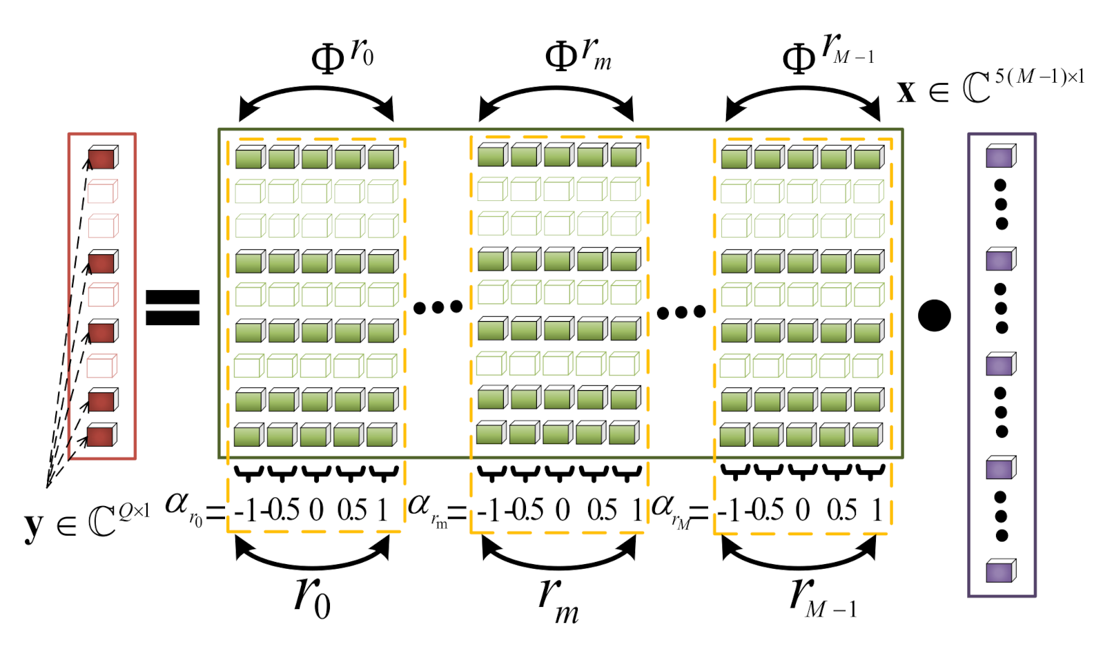
where is the frequency-hopping RCS sequence, is a frequency-hopping index matrix , for , and is an additive noise vector introduced by measurement system. Moreover, is a scattering column vector which contains the scattering intensity, scattering location, and scattering type together. is the dictionary matrix, which can be written as:
where is a sub-matrix of and it consists of five candidate scattering types on the m-th grid. Hence, can be written as:
where is the base of . According to (6) and (8), can be given as:
The schematic diagram of the sparse GTD model in (8) is shown in Figure 2.
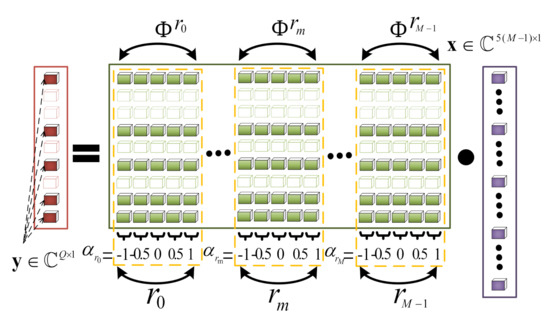
Figure 2.
Diagram of the sparse GTD model.
For simplicity, let us assume the following as:
where represents the frequency-hopping dictionary matrix. Then, (8) can be further rewritten as:
3. Proposed Method
This section consists of three subsections. A non-parametric GTD–SPICE method based on the CMF criterion is introduced in Section 3.1, realizing the advantages of parameter-free and accurate RCS reconstruction. Furthermore, an improved coarse-to-fine two-stage DE–GTD–SPICE method with a lower computational cost is presented in Section 3.2. Furthermore, Section 3.3 summarizes the procedure of the DE–GTD–SPICE method and provides its flowchart.
3.1. GTD–SPICE Method
The goal of SPE is to obtain a set of sparse components to represent the scattering characteristics of radar targets. However, (8) is a linear underdetermined inverse problem, which has an infinite number of solutions. To find a desired solution, the regularization can be used for SPE. However, this optimization problem becomes NP-hard. For simplicity, in (8) can be equivalently transformed to the regularization based on the LASSO framework [36]:
Unlike the regularization, (14) tries to strike a balance between the fidelity and the sparsity. The regularization is convex and computationally efficient, especially when the dictionary matrix is orthogonal. However, the matrix in this paper is not orthogonal, which creates difficulties in solving . In addition, the auxiliary parameter in (14) is also sensitive to the noise and is difficult to be chosen in advance, leading to poor results in practice sometimes.
Instead of adopting regularization, the SPICE algorithm solves by a minimization of the CMF criterion. It is a method without the selection of auxiliary parameters, and has a global convergence [33,34]. According to (8), the covariance of is given as:
where the symbol refers to the expectation operator. The covariance matrix of can be expressed as:
where can be rewritten as:
Note that consists of the frequency-hopping dictionary matrix and the identity matrix of the noise i.e., , together. in (16) can be written as:
For convenience, let
where is composed of the scattering components and the noise components. Once is solved, in (8) is achieved accordingly.
The SPICE algorithm estimates by minimizing the CMF criterion [33,34]:
where is the Hermitian positive definite square root of , and and are the norm and the Frobenius norm, respectively. designates the trace of a square matrix. According to (16) and (18), can be derived as:
Note that , thus the criterion (20) can be simplified to the following minimization problem:
Clearly, the function of (22) is convex, which has a globally optimal solution [34]. In this case, the object is to solve the , not the . Thus, the equivalent minimization problem in (22) with respect to can be derived as:
According to [37,38], the optimal value of can be obtained by cyclic iteration. The iteration process can be as follows:
where denotes the iteration and represents the maximum iterations. Equation (24) and (25) are solved circularly until convergence. In this paper, a matched filter (MF) is used to initialize , which can be determined as follows:
where , is the column of in (17). According to (25), can be determined subsequently. The SPICE algorithm stops when the following condition is satisfied:
where the stopping threshold and maximum iterations T can be set according to the expected accuracy, respectively. The SPICE algorithm for SPE is as follows.
| Algorithm 1. The SPICE algorithm for SPE |
| 1. Input: y, , Δ, T |
| 2. Initialization: |
| 3. while do |
| 4. |
| 5. |
| 6. , |
| 7. end while |
| 8. Output: Scattering parameters vector |
After iterative updating by the SPICE algorithm, the optimal is provided. Since the scattering components and noise components are jointly taken into consideration, and the components after are the noise components which should be removed, only the first data of , i.e., , are kept. Furthermore, in order to extract valid SCs and remove wrong SCs caused by side lobes or existing noise, a threshold function is executed on and it can be reformulated as:
where denotes the element in which represents the valid scattering components, and is a threshold level.
After (28), it can be assumed that all non-zero elements in represent SCs. Hence, the number of SCs i.e., can be determined by counting the number of the non-zero elements in . Then, the SPE, i.e., can be also obtained by matching the base of dictionary matrix one by one. Considering a special case where multiple solved SCs of different scattering types are on the same , these SCs can be synthesized into an equivalent scattering center with the help of (5). Finally, the frequency-hopping RCS sequence can be reconstructed by the formula:
where refers to the number of estimated SCs. More directly, (29) can be written in the form of matrix:
3.2. DE–GTD–SPICE Method
The GTD–SPICE method can accomplish RCS reconstruction, whereas its computational cost is too high due to the large dictionary matrix of the sparse GTD model. To overcome this problem, an improved coarse-to-fine two-stage SPICE method based on the DE model and the GTD model is proposed.
3.2.1. Coarse Estimation of Scattering Location Based on the Sparse DE Model
To predict the candidate distributed location of SCs, the sparse DE model is utilized to model the frequency-hopping RCS sequence. Assume that the coarse range resolution is . In this case, the number of columns is . Similar to (8), the sparse DE model can be reformulated as:
where denotes the scattering parameter on each coarse sampling range grid, and is the Fourier dictionary matrix. According to (7), the element of can be determined by the following formula:
where . The can be set according to the users. On the one hand, if users pay more attention to the computational cost of the coarse stage, the can be set to a small integer. On the other hand, if users are more concerned with the precision of scattering locations, the can be set to a larger integer.
With the help of the SPICE algorithm, the coarse scattering components can also be solved. After a threshold function, the coarse scattering location of SCs can be determined according to . Accordingly, the candidate distributed scattering intervals can be also determined. The diagram is shown in Figure 3.
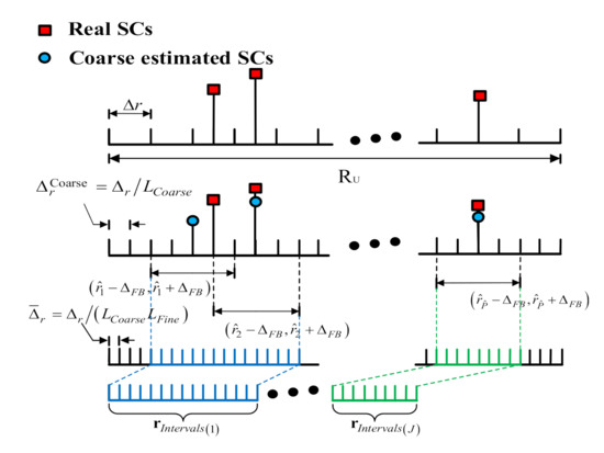
Figure 3.
Diagram of candidate distributed intervals of SCs in the coarse estimation.
Considering the case where there are overlapped regions among coverage subintervals, the final candidate distributed scattering interval can be determined by the following formula as:
where is the coverage radius of scattering center (), the symbol denotes the union operation, are the number of sub-distributed intervals after the union operation, and and denote the starting location and the ending location of the sub-distributed interval, respectively. Only when there is no overlapped region among coverage subintervals can the maximum number of the coarse subsampling grids in be achieved.
3.2.2. Fine Estimation of Scattering Parameter Base on the Sparse GTD Model
Based on in (33), a refined redundant dictionary based on the GTD model can be determined subsequently. Unlike the GTD–SPICE method, which uses a larger dictionary , the DE-GTD model has a refined redundant dictionary that only covers the candidate distributed range of SCs. As a result, the number of columns of is reduced. Assume that there are columns vector in . The subsampling range intervals in the fine stage is assumed as which is set to in this paper. Since , the following formula holds:
In this case, according to (9), the dictionary matrix is completely a subset of the sparse GTD model. On the basis of (33), can be further determined as:
where the symbol denotes the subset operation. Similarly, the sparse DE-GTD model can be written as:
where represents the scattering column vector. When there is no overlapped region among coverage subintervals, the maximum number of subsampling grids can be achieved, and it can be determined by the following formula:
With the sparse DE-GTD model, the fine scattering components can be solved more efficiently. Similar to the solution process in the GTD–SPICE method, the SPE can be also solved. Accordingly, the RCS reconstruction can be accomplished by (29), or by the following formula:
3.3. Procedure of the DE–GTD–SPICE Method
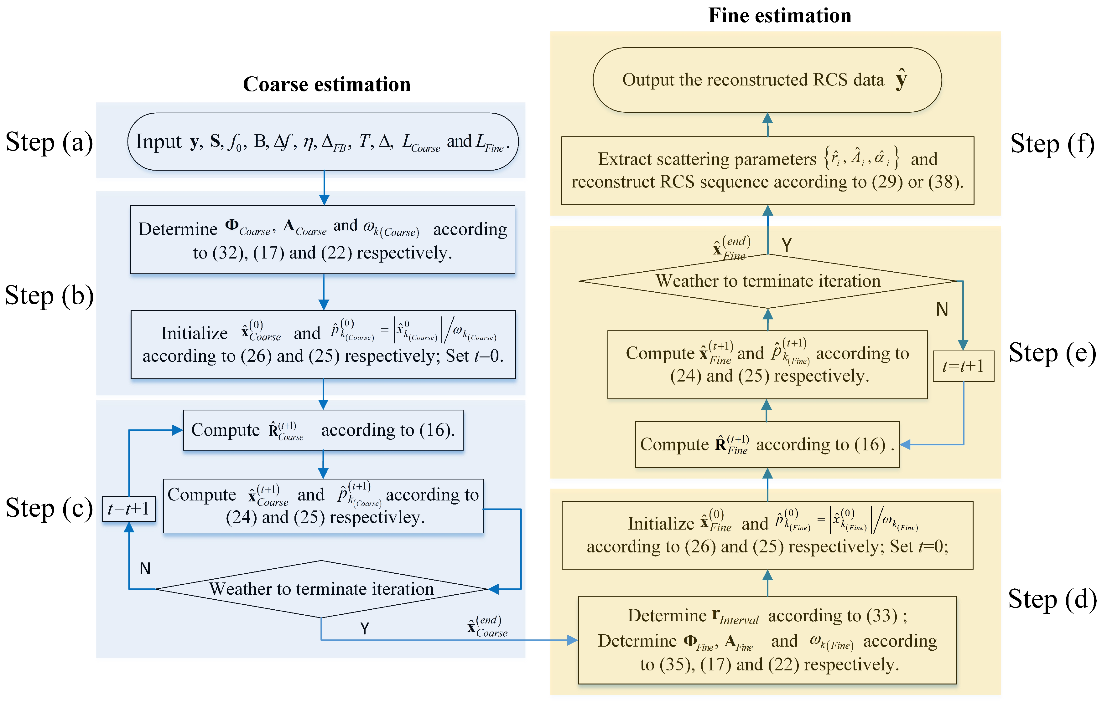
To facilitate the understanding, the flowchart of the DE–GTD–SPICE method is shown in Figure 4.
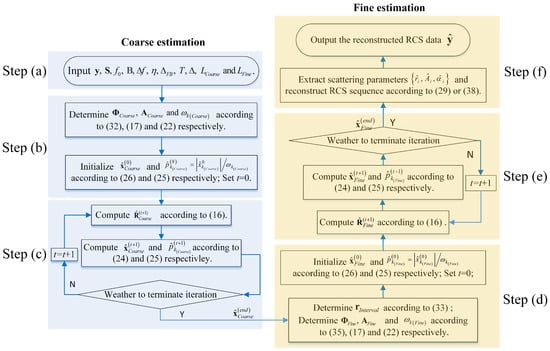
Figure 4.
Flowchart of the proposed DE–GTD–SPICE method.
Accordingly, the flowchart can be summarized as follows:
Step (a). Input.
This step mainly completes the data input. These data are the frequency-hopping sequence , frequency-hopping index matrix , initial frequency , band , frequency interval , truncated threshold , coverage radius , maximum iterations , stopping threshold ,
, and .
Step (b). Initialization of the coarse estimation.
This step aims to prepare the coarse estimation. On the basis of the input, , and are determined according to (32), (17), and (22), respectively. Then, and are initialized according to (26) and (25), respectively.
Step (c). Iteration updating of the coarse estimation.
This step is the key of the coarse estimation. It iteratively updates , , and according to (16), (24), and (25) till convergence. Then, is solved.
Step (d). Initialization of the fine estimation.
Based on the solved , the candidate scattering distributed intervals are determined according to (33). Most importantly, the refined dictionary matrix is generated according to (35). Then, and are also determined. Similarly, and are initialized according to (26) and (25), respectively.
Step (e). Iteration updating of the fine estimation.
This step circularly updates , , and according to (16), (24), and (25), respectively, which aims to solve .
Step (f). Output.
Based on the solved , the SPE results, i.e., are obtained. According to (29) or (38), the RCS reconstruction of the frequency-hopping sequence can be accomplished. Finally, the reconstructed RCS sequence is output.
4. Performance Analysis
In this section, the computational complexity of the two methods is provided. Then, the comparison of the complexity of the two methods are analyzed in detail.
4.1. Complexity of the GTD–SPICE Method
Let us analyze the computational complexity of the GTD–SPICE method. In one iterative loop, (16), (24), and (25) are computed in sequence. For (16), it mainly contains two matrix multiplication operations. Since the sizes of matrix and matrix are and , the first matrix multiplication requires multiplications. The second matrix multiplication is between the intermediate result matrix (after the first matrix multiplication) with size and matrix with size , which requires multiplications. Thus, (16) has a total of multiplications. For (24), it is found that the complexity of matrix operation implemented from right to left is lower than that implemented from left to right. Therefore, we assume that (24) is implemented from right to left. In this case, (24) can be decomposed into these matrix operations: the inversion of a matrix; matrix multiplication of a matrix and a column vector; matrix multiplication of a matrix and a column vector; and matrix multiplication of a matrix and a column vector. The multiplications of the four matrix multiplications are , , , and , respectively. Thus, (24) requires a total of multiplications. For (25), it can be considered as multiplication operations, where multiplications are required.
The total multiplications of the GTD–SPICE method are the sum of those of (16), (24), and (25). Assume that the GTD–SPICE method needs iterations to converge. Therefore, the computational complexity of the GTD–SPICE method can be calculated as:
For the convenience of analysis, substituting and into (39), can be approximated as:
In the approximation of (40), the relation .
4.2. Complexity of the DE–GTD–SPICE Method
Let us further analyze the complexity of the DE–GTD–SPICE method. Assume that the coarse estimation and the fine estimation converges after and iterations, respectively. In the coarse estimation, the number of columns of ( and ) is . Similarly, the complexity of the coarse estimation can be calculated as:
Substituting and , can be approximated as:
In the approximation of (42), the relation . In the fine estimation, the number of columns of and is . Similar to (39), the complexity of the fine estimation can be given as:
Substituting and into (43), the complexity of the fine estimation can be reformulated as:
For a more concise approximation, assume (). Then, (44) can be further rewritten as:
In the approximation of (45), the relation . The total of the DE–GTD–SPICE method is the sum of (42) and (45), which can be calculated as:
Due to the sparse distribution of SCs, is always satisfied. If the coarse estimation is accurate, i.e., , we have . In this case, is almost a constant, and . However, if the coarse estimation is inaccurate, may become large. In this case, is not satisfied and the computational complexity of the fine estimation subsequently increases.
4.3. Comparison of Complexity
Next, let us compare the complexity of the two methods. For simplicity, let us assume . According to (34), (40), and (46), the ratio of the complexity of the two methods, i.e., , can be calculated as:
Equation (47) shows that, with the fixed and , increases with the increase of . When , (47) can be reduced to . Since and are set to positive integers in this paper, holds, and its maximum is achieved when . Therefore, when , the complexity of the DE–GTD–SPICE method is much lower than that of the GTD–SPICE method. More generally, the complexity of DE–GTD–SPICE is lower than that of GTD–SPICE only under the condition of i.e., .
5. Experiments
In this section, experiments are performed to verify the validity of the proposed methods. To make it more convincing, experiments in different frequency-sweeping intervals , SNRs, and FHRs are carried out. In addition, the iteratively reweighted least squares method (GTD–IRLS) [39] and the LASSO-based -norm method (GTD–CVX) are used for comparison. These methods are all implemented on a PC with an Intel i5-4210U CPU and 8GB RAM.
5.1. Evaluation Metrics
To quantify the accuracy of the amplitude of the reconstructed RCS sequence , the mean square error (MSE) of amplitude, i.e., , is defined as:
where is the n-th element in . To quantify the accuracy of the phase of , the MSE of the phase, i.e., , is defined as:
For a fairer assessment, a correlation function (COR) which can reflect the similarity between the reconstructed RCS sequence and the true RCS sequence is defined as:
where . The closer is to 1, the more similar the reconstructed RCS sequence is to the true RCS sequence, and the higher the quality of RCS reconstruction.
5.2. Experimental Results
Assume that the radar target consists of five SCs, and the scattering parameters are set according to Table 1. In this case, the parameters of the radar system are set as follows:, , and . Accordingly, the number of stepped frequency points is , the normal range resolution is , and the maximum unambiguous range is . The subsampling range interval is set to (L = 4). For easy reference, the radar parameters are listed in Table 2. The simulated data is obtained based on (2). In order to provide a benchmark, the GTD–CVX method and GTD–IRLS method are used. Therefore, the GTD–SPICE method, the DE–GTD–SPICE method, the GTD–IRLS method and the GTD–CVX method are included in the following experiments.

Table 1.
Scattering parameters of the five SCs.

Table 2.
Radar system parameters.
5.2.1. Validation of the Proposed Methods
First, let us validate the effectiveness of the proposed methods under different SNR conditions. In this experiment, the FHR is fixed to 60%, and the SNR is set to 25 dB and 5 dB, respectively. Note that the auxiliary parameter of the GTD–CVX method is chosen as and , respectively. Figure 5 shows the SPE results of the GTD–SPICE, DE–GTD–SPICE, the GTD–IRLS, and the GTD–CVX method at 25 dB and 5 dB, respectively.
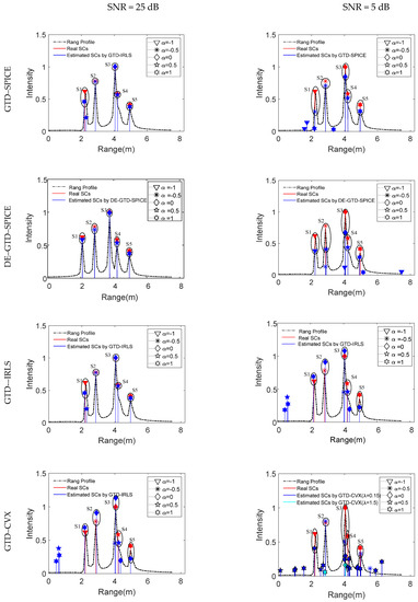
Figure 5.
SPE results of the GTD–SPICE, DE–GTD–SPICE, GTD–IRLS, and GTD–CVX method. In this case, FHR = 60%, , and in the DE–GTD–SPICE method.
It is seen in Figure 5 that the SPE results of the four methods at 25 dB are more precise than those at 5 dB. When SNR = 25 dB, the parameters extracted by the GTD–SPICE method and the DE–GTD–SPICE method are consistent with their true values. The scattering locations and scattering types of the five SCs are all estimated correctly. As shown in the first column of Figure 5, the intensities of the five SCs obtained by the DE–GTD–SPICE method are closer to their true values than those obtained by the GTD–SPICE method. The mean error of the scattering intensities of the five SCs of the DE–GTD–SPICE method is 0.09, whereas the mean error of the GTD–SPICE method is 0.13. In particular, the scattering intensity of S3 (0.99) estimated by the DE–GTD–SPICE method is quite close to its true value (1.00), and it has the least deviation.
In contrast, the SPE results of the other two methods are less accurate. Though the parameters of S2, S3, S4, and S5 are extracted correctly by the GTD–IRLS method, the scattering intensity and scattering type of S1 are misestimated as and , respectively. Also, there is a little deviation in the scattering location of S1, and there is also a fake scattering center near S1. The results of the GTD–CVX method are sensitive to the auxiliary parameter . When , the SPE results of S1, S2, S3, and S4 are all correct, and only the scattering type and scattering intensity of S1 are inaccurate. The scattering type of S1 is misjudged as , and there is a deviation of about 0.09 in the scattering intensity of S1. When , the SPE results are the poorest. The maximum deviation of the scattering intensity occurs at S2, and its relative error is over 80%. In addition, S5 is not contained in its results.
Compared with the case of SNR = 25 dB, the SPE results of the four methods under SNR = 5 dB are poorer. The SPE results of the five SCs by the GTD–SPICE method are basically consistent with the true values. It is seen that the scattering locations of the five SCs are correctly extracted. The scattering types of S2, S3, S4, and S5 are correctly judged, except that the scattering type of S1 is misjudged as . The scattering intensities of S2, S3, S4, and S5 are also close to their true values. The deviation of the estimated scattering intensity of S1 is up to 0.31, which is the maximum deviation among all SCs. In addition, there are four fake estimated SCs whose intensities are smaller than 0.1. The SPE results obtained by the DE–GTD–SPICE method are less accurate than that of the GTD–SPICE method. The scattering locations and scattering types of the five SCs are correctly estimated; however, the deviations of the scattering intensities of the five SCs are all larger than 0.1, and the maximum deviation of the estimated scattering intensity reaches 0.34. Also, there are four fake estimated SCs.
The scattering locations and scattering intensity of the five SCs extracted by the GTD.IRLS method are basically consistent with their true values, and the mean error of their scattering intensities is 0.15. Also, the scattering type of S1 and S2 is misjudged as and , respectively. When , the GTD–CVX method correctly estimates S2, whereas the scattering types of S1, S3, S4, and S5 are misjudged as , , and , respectively. The maximum deviation of the scattering intensity of the five SCs occurs at S3, up to 0.52. In addition, the result contains eighteen wrong SCs. When , due to strong noise, the method can only extract two SCs whose locations may be correct. However, the estimated scattering intensities are far from their true values. This indicates that the estimated results are totally wrong.
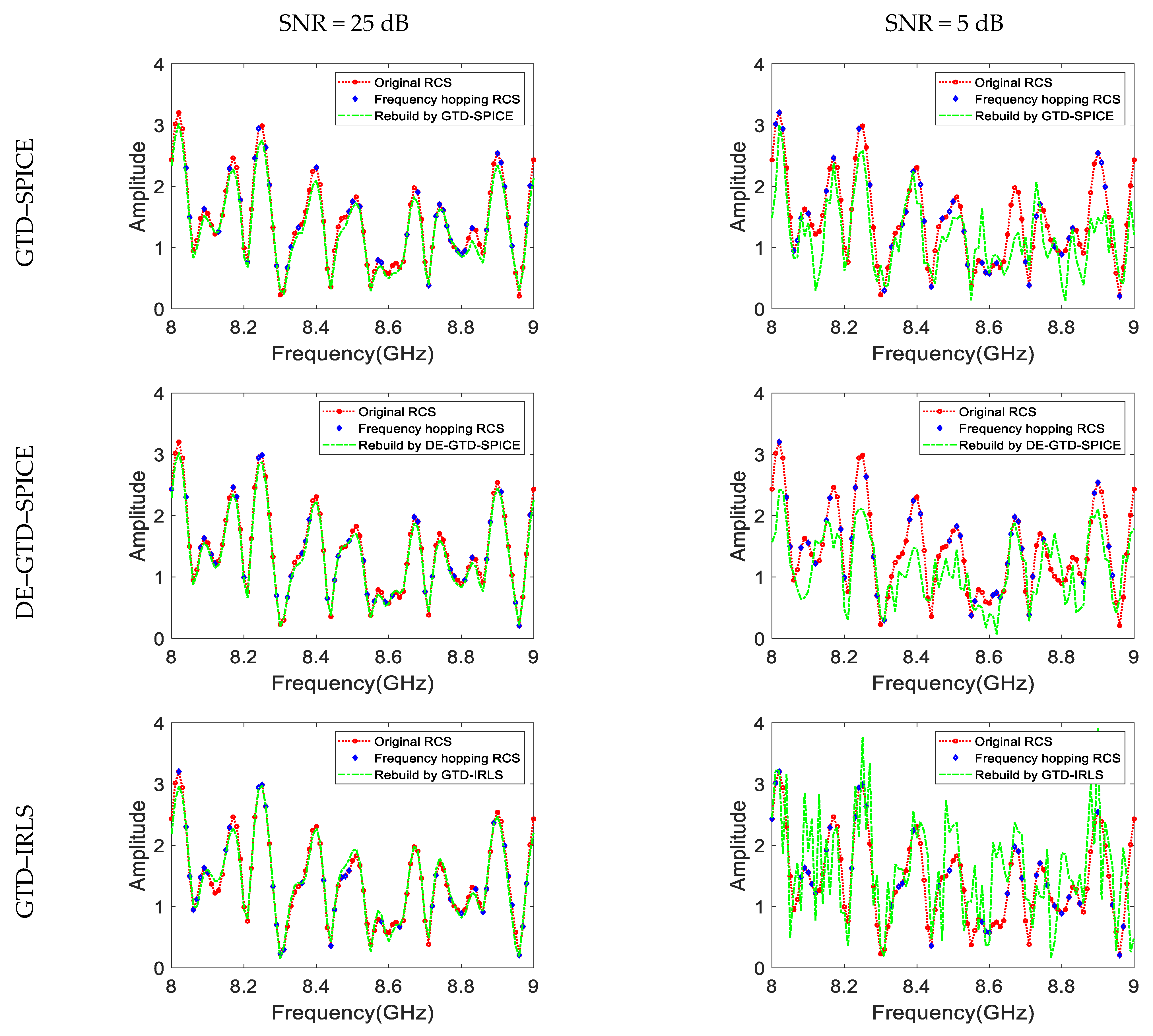
Based on the estimated scattering parameters, the RCS sequence can be reconstructed. Figure 6 shows the amplitude of the reconstructed RCS sequence of the four methods. It is seen that the reconstruction results at 25 dB are more accurate than those at 5 dB. When SNR = 25 dB, the performance of the GTD–SPICE method, DE–GTD–SPICE method, GTD–IRLS method, and the GTD–CVX () method are comparable, and the reconstructed RCS sequences are close to the true RCS sequence. In contrast, the GTD–CVX () method cannot reconstruct the RCS sequence well. The amplitude of the reconstructed sequence has a large deviation from the true RCS sequence. These results are consistent with the poor SPE results of the GTD–CVX () method in Figure 5.
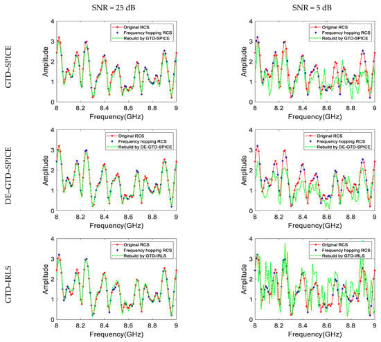

Figure 6.
Amplitude of the reconstructed RCS sequence using the GTD–SPICE, DE–GTD–SPICE, GTD–IRLS, and GTD–CVX methods. In this case, FHR = 60%,, and in the DE–GTD–SPICE method.
When SNR = 5 dB, the reconstruction results of the four methods are poorer. As shown in the second column of Figure 6, the performance of the GTD–SPICE method, DE–GTD–SPICE method, GTD–IRLS method, and GTD–CVX () method seems to be comparable as well. It is seen that there are large deviations near the peak position of the reconstructed RCS sequence by the four methods. Similarly, the reconstructed RCS sequence by the GTD–CVX () method is greatly deviated from the true RCS sequence. It is the poorest result.
To quantitatively compare the performance of the four methods, , ,, and the computational time are given in Table 3. Since the GTD–SPICE () method has the poorest results, its metrics are not provided. When SNR = 25 dB, the ,, of the GTD–SPICE method, DE–GTD–SPICE method, and GTD–CVX () method are almost equal to each other, respectively. Although the GTD–IRLS method has the minimum , i.e., , it has the maximum , i.e., , and minimum , i.e., . This indicates that the accuracy of the reconstructed RCS sequence by the GTD–SPICE method, the DE–GTD–SPICE method, and the GTD–CVX () method is basically similar, and the accuracy of the reconstructed RCS sequence by the GTD–IRLS method is slightly lower. When SNR = 5 dB, the GTD–SPICE method has the minimum , i.e., , the minimum , i.e., , and the maximum , i.e., . In contrast, the GTD–IRLS method has the maximum , i.e., , the maximum , i.e., , and the minimum , i.e., . These metrics show that in this case, the GTD–SPICE method has the best reconstructed RCS sequence, whereas the GTD–IRLS method has the poorest reconstruction results.

Table 3.
Numerical results under different SNR conditions.
Then, let us compare the computational time. The GTD–SPICE method has the longest computational time of about 30 s under the two SNR conditions. In contrast, the DE–GTD–SPICE method has the shortest time of 2.2969 s at 25 dB. Compared with the GTD–SPICE method, the computational time is reduced by more than 26 s (larger than 90%). This validates the effectiveness of the DE–GTD–SPICE method in reducing the computational time compared to the GTD–SPICE method. Moreover, it is more than 4 s and 6 s faster than the GTD–CVX () method and the GTD–IRLS method, respectively. When SNR = 5 dB, though the computational time of the DE–GTD–SPICE method increases to 18.5156 s, it is still faster than the GTD–SPICE method. The GTD–SPICE method takes almost three times as long as the GTD–CVX () method. Therefore, the computational time of the DE–GTD–SPICE method may be related to SNR, and the computational time of the GTD–SPICE algorithm may be independent of the SNR.
5.2.2. Performance Versus
The frequency-sweeping interval determines the maximum unambiguous distance () and the number of stepped frequency points . Thus, plays a role in the accuracy of RCS reconstruction.
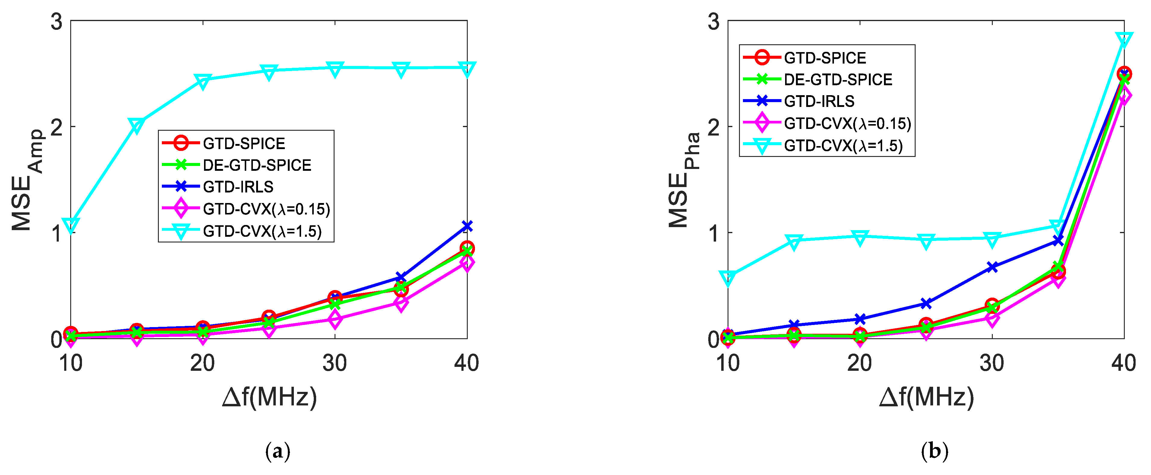
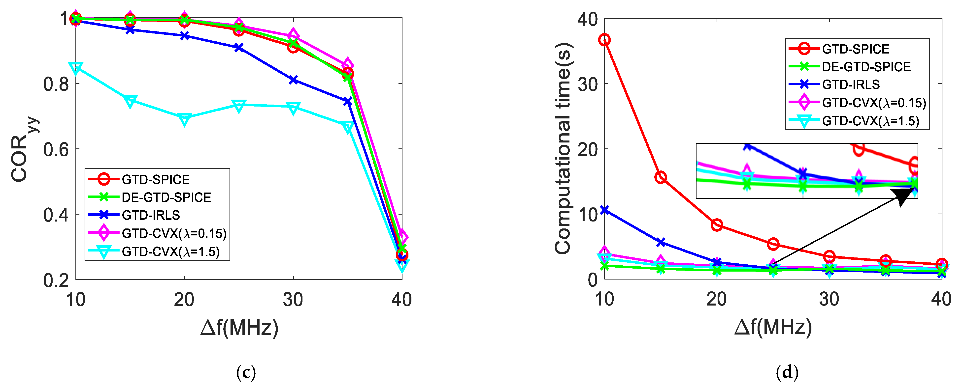
First, let us compare the performance of the four methods under different . In this experiment, the SNR and FHR are fixed to 30 dB and 60%, respectively. The Monte Carlo simulation with 50 trials is used. The ranges from 10 MHz to 40 MHz with an interval of 5 MHz. The averages of the , , , and computational time versus are shown in Figure 7a–d, respectively.
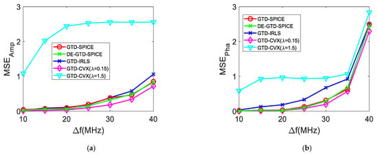

Figure 7.
Comparison on (a) MSE of the amplitude of the reconstructed RCS sequence, (b) MSE of the phase of the reconstructed RCS sequence, and (c) the correlation coefficient versus the . (d) Computational time versus .
It can be seen in Figure 7a–c that the and increase with the increase of , and the of the four methods decreases with the increase of . It is seen that the GTD–CVX () method is more accurate than the GTD–CVX () method, due to the fact that it has much smaller , , and larger . This indicates that the selection of auxiliary parameter is the key to the performance of the GTD–CVX method. For simplicity, unless specifically illustrated, the GTD–CVX method refers to the GTD–CVX () method in the following.
When , the ,, and of the four methods are almost the same, respectively, which indicates the comparable performance in RCS reconstruction. It is seen in Figure 7a that when , the of the GTD–SPICE method and the DE–GTD–SPICE method is slightly less than that of the GTD–IRLS method, and a little bigger than that of the GTD–CVX method. Figure 7b shows that the of the GTD–SPICE method, the DE–GTD–SPICE method, and the GTD–CVX method is quite close, and it is less than that of the GTD–IRLS method. As shown in Figure 7c, the of the GTD–SPICE method, the DE–GTD–SPICE method, and the GTD–CVX method is almost the same, and it is larger than that of the GTD–IRLS method. Therefore, it can be inferred that the GTD–SPICE method, the DE–GTD–SPICE method, and the GTD–CVX method can have a comparable performance at all , and a better performance than the GTD–IRLS method when is large.
As shown in Figure 7d, with the increase of , the computational time of the GTD–SPICE method, the GTD–IRLS method, and the GTD–CVX method gradually decreases. This is due to their computational complexity decreases with the decrease of , which is consistent with (40). The GTD–SPICE method requires the longest computational time of about 37s when . It is more than three times and six times of that of the GTD–IRLS method and the GTD–CVX method, respectively. When ranges from 10 MHz to 30 MHz, the maximum computational time of the DE–GTD–SPICE method is about 3 s, which is only around 8.12% of that of the GTD–SPICE method, which indicates that the DE–GTD–SPICE method can reduce computational time compared with the GTD–SPICE method. It is also seen that when , the computational time of the DE-GTD method has a slight increase as the increase of . The reason for this phenomenon will be explained in Section 5.2.4.
5.2.3. Performance Versus SNR
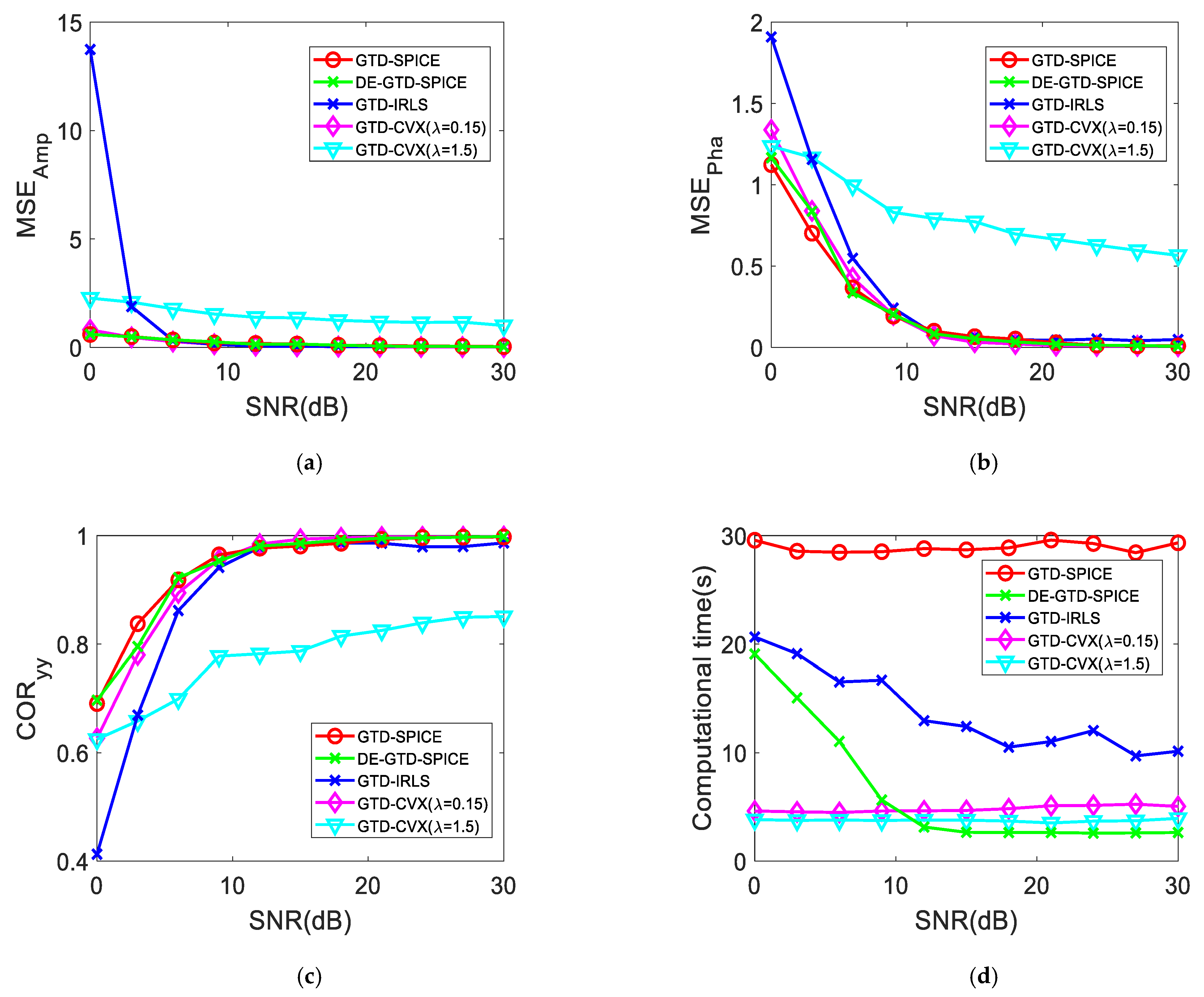
Let us further compare the performance of the four methods under different SNRs. In this experiment, the and the FHR are fixed to 10 MHz and 60%, respectively. The Monte Carlo simulation with 50 trials is used. The SNR ranges from 0 dB to 30 dB with an interval of 3 dB. The averages of the ,,, and computational time versus SNR are shown in Figure 8a–d, respectively.
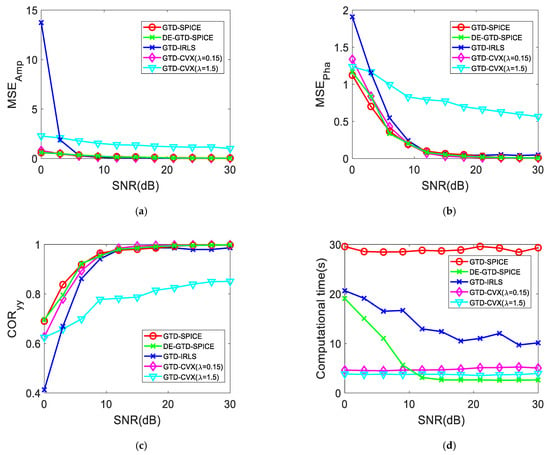
Figure 8.
Comparison on (a) MSE of the amplitude of the reconstructed RCS sequence, (b) MSE of the phase of the reconstructed RCS sequence, and (c) the correlation coefficient versus the SNR. (d) Computational time versus the SNR.
As shown in Figure 8a–c, the and decrease with the increase of SNR, and the of the four methods increases with the increase of SNR. It can be seen that the performance of the GTD–CVX () method is worse than that of the GTD–CVX () method due to it has larger , , and smaller . This also means that the GTD–CVX method is sensitive to the auxiliary parameter .
As can be seen in Figure 8a, when SNR < 6 dB, the of the GTD–SPICE method, the DE–GTD–SPICE method, and the GTD–CVX method is much smaller than that of the GTD–IRLS method. When SNR > 6 dB, the of the four methods is almost the same. As shown in Figure 8b, when SNR < 12 dB, the of both the GTD–SPICE method and DE–GTD–SPICE method is slightly smaller than that of the GTD–CVX method and much smaller that of the GTD–IRLS method. In contrast, when SNR > 12 dB, the of the four methods is quite close and tends to be 0, except that the of the GTD–IRLS method is slightly larger than 0 when SNR is from 20 to 30 dB. It is seen in Figure 8c that when SNR < 10 dB, the of the GTD–SPICE method and the DE–GTD–SPICE method is slightly larger than that of the GTD–CVX method and much larger than that of the GTD–IRLS method. When SNR > 10 dB, the of the four methods is almost equal and quite close to 1, except that the of the GTD–IRLS methods is a little smaller than 1 when SNR is from 20 to 30 dB.This indicates that the two proposed methods outperform both the GTD–CVX method and the GTD–IRLS method under low SNR conditions, and have a slight advantage under high SNR conditions.
As shown in Figure 8d, when SNR ranges from 0 dB to 30 dB, the computational time of the GTD–SPICE method and the GTD–CVX method is almost a constant. The GTD–SPICE method has the longest computational time of approximately 30 s, and the GTD–CVX method has a computational time of about 6s. The computational time of the GTD–IRLS method is in the middle and decreases with the increase of SNR. Also, it can be seen that the computational time of the DE–GTD–SPICE method decreases with the increase of the SNR under the condition of SNR being 0~13 dB. Since severe noise affects the accuracy of the coarse estimation, the estimation of the number of SCs, i.e., , becomes larger. Accordingly, also becomes larger, which increases the computational complexity of the fine estimation. This is consistent with (46). Although the computational time of the DE–GTD–SPICE method has the maximum, around 20 s at SNR = 0 dB, it is only about 66.7% of that of the GTD–SPICE method. When SNR > 13 dB, its computational time tends to be stable and approaches 3 s, which is only about 10% of that of the GTD–SPICE method (30 s). Substituting and into (47), we can have . This is basically consistent with 10%, which validates the effectiveness of the DE–GTD–SPICE method in reducing the computational cost.
5.2.4. Performance Versus FHR
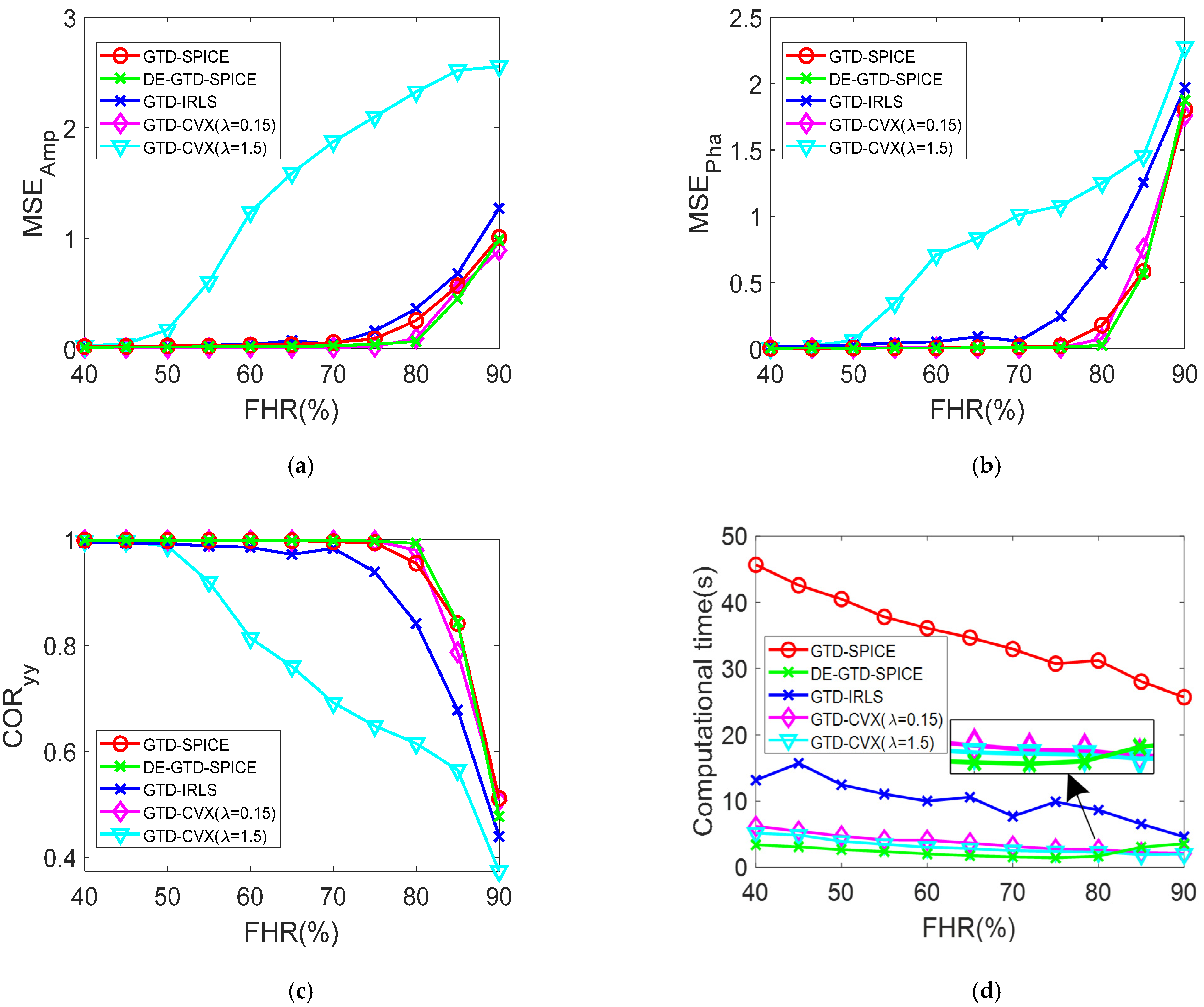
Next, we compare the performance of the four methods in different FHRs. The and SNR are fixed to 10 MHz and 30 dB, respectively. Similarly, the Monte Carlo simulation with 50 trials is used. The FHR ranges from 40% to 90% with an interval of 5%. The averages of the , , , and computational time are shown in Figure 9a–d, respectively.
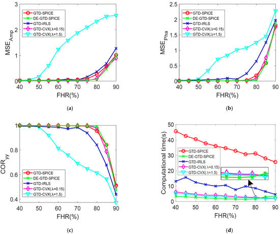
Figure 9.
Comparison on (a) MSE of the amplitude of the reconstructed RCS sequence, (b) MSE of the phase of the reconstructed RCS sequence, and (c) the correlation coefficient versus the FHR. (d) Computational time versus the FHR.
It can be seen in Figure 9a–c that the and increase with the increase of FHR, and the of the four methods decreases with the increase of the FHR. It is seen that the GTD–CVX () method is much more accurate than the GTD–CVX () method. This also shows that the selection of the auxiliary parameter is the key to the performance of the GTD–CVX method.
When , the , , and of the four methods are quite close, respectively, which indicates the comparable performance in RCS reconstruction. It is seen in Figure 9a when that the of the GTD–SPICE method, the DE–GTD–SPICE method, and the GTD–CVX method is close and slightly smaller than that of the GTD–IRLS method. Figure 9b also shows the similar relation of the of the four methods. When , the of the GTD–SPICE method, the DE–GTD–SPICE method, and the GTD–CVX method is basically close, and is smaller to that of the GTD–IRLS method. As shown in Figure 9c, when , the of the GTD–SPICE method, the DE–GTD–SPICE method, and the GTD–CVX method is almost the same, whereas the of the GTD–IRLS method is smaller than that of the other three methods. Therefore, the four methods have comparable performance in low FHRs, while the proposed methods outperform the GTD–IRLS method under high FHR conditions.
It can be also found that when , the , , and of the four methods all change dramatically, which is due to the destruction of RIP conditions. According to [40], the minimum number of scattering measurement points can be determined theoretically. According to [41], for a reliable recovery, can be calculated as . As shown in Figure 9a–c, the low boundary of FHR is approximately 80%. Hence, the number of frequency-hopping points in actual is , i.e., , which is basically consistent with the theoretical low boundary .
As shown in Figure 9d, with the increase of FHR, the computational time of the GTD–SPICE method, the GTD–IRLS method, and the GTD–CVX method gradually decreases. This is due to the fact that their computational complexity decreases with the decrease of , which is consistent with (39). The GTD–SPICE method requires the longest computational time of about 30 s at FHR = 40% among the four methods. When FHR ranges from 40% to 75%, the computational time of DE–GTD–SPICE method decreases with the decrease of FHR, on the premise of guaranteeing the accuracy of RCS reconstruction. This is also due to the complexity of the DE–GTD–SPICE method, which decreases with the decrease of . Moreover, it has the least computational time of about 3 s at FHR = 75%, which is about 10% of that of the GTD–SPICE method (about 30 s). This is also consistent with (47). In contrast, when FHR > 75%, its computational time begins to increase, whose phenomenon also occurs at Figure 7d. This is the result of the FHR approaching the RIP condition. In this case, the coarse estimation obtains a larger number of SCs than that of the true value and becomes larger, which increases the computational complexity of the fine estimation. This is consistent with (46), in which the increase of will increase the computational complexity.
5.2.5. Joint Experiment on Different SNRs and FHRs
Lastly, the joint impacts of , SNR, and FHR on the proposed methods in RCS reconstruction are analyzed. Since the performance of the GTD–SPICE method and the DE–GTD–SPICE method in RCS reconstruction is related to , SNR, and FHR, it is difficult to determine which , SNR, and FHR are more efficient. Considering the above findings that the performance of the proposed method has similar trends in terms of and FHR, only the SNR and FHR are performed jointly in this experiment. The SNR ranges from 10 dB to 30 dB with an interval of 4 dB, and the FHR ranges from 40% to 90% with an interval of 5%. Similarly, the Monte Carlo simulation with 50 trials is used. The averages of the and the computational time of the two proposed methods are shown in Figure 10a–d, respectively.
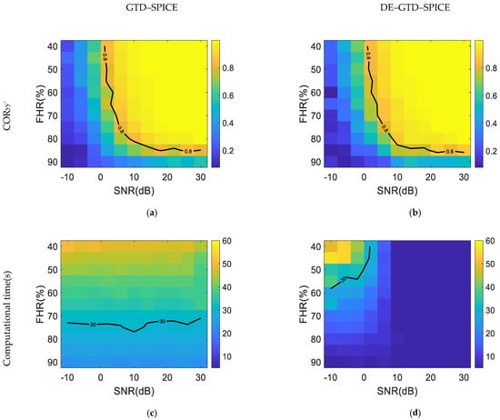
Figure 10.
The averages of the and computational time(s): (a) averaged of the GTD–SPICE method, (b) averaged of the DE–GTD–SPICE method, (c) computational time of the GTD–SPICE method, and (d) computational time of the DE–GTD–SPICE method.
As shown in Figure 10a–b, the of the two proposed methods is quite close under the same SNR and FHR. When SNR > 8 dB and FHR < 80%, the of the two methods is larger than 0.8, which shows superior performance in RCS reconstruction. Then, let us further compare its computational time. It can be seen in Figure 10c that the computational time of the GTD–SPICE method significantly depends on FHR. When FHR < 75%, its computational time is larger than 30 s. In contrast, the computational time of the DE–GTD–SPICE method is affected by both the SNR and FHR. It is seen in Figure 10d that only when SNR < 0 dB and FHR < 50%, the computational time of the DE–GTD–SPICE method is larger than 30s. From Figure 10c–d, it can be found that the DE–GTD–SPICE method has a shorter time and a higher efficiency than the GTD–SPICE method. Therefore, it can be concluded that both the methods are reliable and effective for RCS reconstruction. In particular, the DE–GTD–SPICE method requires less computational time.
6. Conclusions
In this paper, a random frequency-hopping pattern combined with RCS reconstruction is utilized to reduce the time of the coherent stepped frequency scattering measurement in anechoic chambers. To achieve accurate RCS reconstruction, the non-parametric GTD–SPICE method and the DE–GTD–SPICE method are proposed. Then, the computational complexity of the two methods is analyzed in detail.
Numerical simulations on different , SNRs, and FHRs are carried out to evaluate their performance, respectively. The GTD–CVX method and the GTD–IRLS method are used for comparison. Results show that the performance of the GTD–SPICE method and the DE–GTD–SPICE method are comparable to the GTD–CVX method, with the best auxiliary parameter, which outperforms the GTD–IRLS method. However, the GTD–CVX is sensitive to the auxiliary parameter. Without a good selection of the auxiliary parameter, its RCS reconstruction result is poor and cannot be used. Compared with the GTD–CVX method, the proposed GTD–SPICE method and the DE–GTD–SPICE method are non-parametric. Thus, the two methods can accomplish reliable RCS reconstruction. In addition, both the methods can achieve accurate RCS reconstruction.
Therefore, the frequency-hopping pattern combined with RCS reconstruction can reduce the measurement time in anechoic chambers, which has wide application prospects in RCS measurement. Next, measured data will be used for further research.
Author Contributions
All authors have made substantial contributions to this work. Y.L. (Yingjun Li) performed the experiments, produced the results, and finished writing the original draft; W.Z. participated in the experiment implementation and edited the draft; B.T. conceived the idea; W.L. took part in the discussion of the method and the results; Y.L. (Yongxiang Liu). reviewed the draft, analyzed the results, gave constructive suggestions and provided the funding. All authors have read and agreed to the published version of the manuscript.
Funding
This work was partly supported by the National Natural Science Foundation of China (61901481, 61921001, 61901487) and Hunan Provincial Natural Science Foundation of China (2021JJ20056).
Institutional Review Board Statement
Not applicable.
Informed Consent Statement
Not applicable.
Data Availability Statement
The data presented in this study are available on request from the corresponding author.
Acknowledgments
The authors would like to thank all those who gave valuable help and suggestions to this manuscript, which were essential to the outcome of this paper.
Conflicts of Interest
The authors declare no conflict of interest.
References
- Knott, E.F.; Schaeffer, J.F.; Tulley, M.T. Radar Cross Section, 2nd ed.; SciTech: Raleigh, NC, USA, 2004. [Google Scholar]
- Odendaal, J.W.; Joubert, J. Radar cross section measurements using near-field radar imaging. IEEE Trans. Instrum. Meas. 1996, 45, 948–954. [Google Scholar]
- Bae, J.H.; Kang, B.S.; Kim, K.T.; Yang, E. Performance of sparse recovery algorithms for the reconstruction of radar images from incomplete RCS data. IEEE Geosci. Remote. Sens. Lett. 2014, 12, 860–864. [Google Scholar]
- Dudgeon, D.E.; Lacoss, R.T. An Overview of Automatic Target Recognition. 1993. Available online: http://citeseerx.ist.psu.edu/viewdoc/download?doi=10.1.1.186.2998&rep=rep1&type=pdf (accessed on 9 September 2021).
- Tan, Q.J.O.; Romero, R.A.; Jenn, D.C. Target recognition with adaptive waveforms in cognitive radar using practical target RCS responses. In Proceedings of the IEEE Radar Conference, Oklahoma City, OK, USA, 23–27 April 2018; pp. 0606–0611. [Google Scholar]
- Fan, J.; Tomas, A. Target Reconstruction Based on Attributed Scattering Centers with Application to Robust SAR ATR. Remote Sens. 2018, 10, 655. [Google Scholar]
- Borkar, V.G.; Ghosh, A.; Singh, R.K.; Chourasia, N.K. Radar cross-section measurement techniques. Def. Sci. J. 2010, 60, 204. [Google Scholar]
- Hu, S.; Law, C.L.; Dou, W. Measurements of UWB antennas backscattering characteristics for RFID systems. In Proceedings of the IEEE International Conference on Ultra-Wideband, Singapore, 24–26 September 2007; pp. 94–99. [Google Scholar]
- Levitas, B.; Matuzas, J.; Drozdov, M. UWB time domain system for RCS measurements. In Proceedings of the IEEE 13th International Radar Symposium, Warsaw, Poland, 23–25 May 2012; pp. 241–244. [Google Scholar]
- Mihai, I.V.; Tamas, R.; Sharaiha, A. An UWB Physical Optics Approach for Fresnel-Zone RCS Measurements on a Complex Target at Non-Normal Incidence. Sensors 2019, 19, 5454. [Google Scholar]
- Glaser, J.I. Some results in the bistatic radar cross section (RCS) of complex objects. Proc. IEEE 1989, 77, 639–648. [Google Scholar]
- Yukhanov, Y.; Orda-Zhigulina, M.; Merglodov, I.; Ilyin, I.; Kostromitin, G. Measurements of monostatic and bistatic radar cross section in anechoic chamber. In Proceedings of the IEEE 14th International Radar Symposium (IRS), Dresden, Germany, 19–21 June 2013; pp. 947–952. [Google Scholar]
- Keller, J.B. Geometrical theory of diffraction. Josa 1962, 52, 116–130. [Google Scholar]
- Potter, L.; Chiang, D.-M.; Carriere, R.; Gerry, M. A GTD-based parametric model for radar scattering. IEEE Trans. Antennas Propag. 1995, 43, 1058–1067. [Google Scholar]
- Hurst, M.; Mittra, R. Scattering center analysis via Prony’s method. IEEE Trans. Antennas Propag. 1987, 35, 986–988. [Google Scholar]
- Carriere, R.; Moses, R.L. High resolution radar target modeling using a modified Prony estimator. IEEE Trans. Antennas Propag. 1992, 40, 13–18. [Google Scholar]
- Pepin, M.P.; Clark, M.P.; Li, J. On the applicability of 2-D damped exponential models to synthetic aperture radar. In Proceedings of the International Conference on Acoustics, Speech, and Signal Processing, Detroit, MI, USA, 9–12 May 1995; pp. 2149–2152. [Google Scholar]
- Zhang, S.; Liu, Y.; Li, X. Fast Sparse Aperture ISAR Autofocusing and Imaging via ADMM Based Sparse Bayesian Learning. IEEE Trans. Image Process. 2019, 29, 3213–3226. [Google Scholar]
- James, G.L. Geometrical Theory of Diffraction for Electromagnetic Waves, 3rd ed.; IET: London, UK, 1986. [Google Scholar]
- Hua, Y. Estimating two-dimensional frequencies by matrix enhancement and matrix pencil. IEEE Trans. Signal Process. 1992, 40, 2267–2280. [Google Scholar]
- Zheng, S.; Zhang, X.; Zhao, W.; Zhou, J.; Zong, B.; Xu, J. Parameter estimation of GTD model and RCS extrapolation based on a modified 3D-ESPRIT algorithm. J. Syst. Eng. Electron. 2020, 31, 1206–1215. [Google Scholar]
- He, Z.; Zhang, X.; Li, X.; Zhuan, G.Z. A new Method for Parameter Estimation of GTD Model. J. Electron. Inf. Technol. 2005, 9, 1679–1682. (In Chinese) [Google Scholar]
- Bresler, Y.; Macovski, A. Exact maximum likelihood parameter estimation of superimposed exponential signals in noise. IEEE Trans. Acoust. Speech, Signal Process. 1986, 34, 1081–1089. [Google Scholar]
- Shi, Z.; Zhou, J.; Zhao, H. A GTD Scattering center model parameter estimation method based on CPSO. Acta Electron. Sin. 2007, 35, 1102–1107. (In Chinese) [Google Scholar]
- Li, W.; Xu, Y.; Tang, J. A multi-objective resolution method based on RELAX algorithm. Digit. Technol. Appl. 2017, 3, 139–141. [Google Scholar]
- Nguyen, L.H.; Tran, T.; Do, T. Sparse models and sparse recovery for ultra-wideband SAR applications. IEEE Trans. Aerosp. Electron. Syst. 2014, 50, 940–958. [Google Scholar]
- Su, W.; Wang, H.; Yang, Z. Synthetic aperture radar imaging based on attributed scatter model using sparse recovery techniques. J. Cent. South Univ. 2014, 21, 223–231. [Google Scholar]
- Bae, J.-H.; Kang, B.-S.; Yang, E.; Kim, K.-T. Compressive sensing-based algorithm for one dimensional scattering center extraction. Microw. Opt. Technol. Lett. 2016, 58, 1408–1415. [Google Scholar]
- Liu, H.; Jiu, B.; Li, F.; Wang, Y. Attributed scattering center extraction algorithm based on sparse representation with dictionary refinement. IEEE Trans. Antennas Propag. 2017, 65, 2604–2614. [Google Scholar]
- Tropp, J.A.; Gilbert, A.C.; Strauss, M.J. Algorithms for simultaneous sparse approximation. Part I: Greedy pursuit. Signal Process. 2006; 86, 572–588. [Google Scholar]
- Tropp, J.A. Algorithms for simultaneous sparse approximation. Part II: Convex relaxation. Signal Process. 2006, 86, 589–602. [Google Scholar]
- Tipping, A.; Faul, A. Analysis of sparse Bayesian learning. Adv. Neural Inf. Process. Syst. 2002, 14, 383–389. [Google Scholar]
- Ottersten, B.; Stoica, P.; Roy, R. Covariance Matching Estimation Techniques for Array Signal Processing Applications. Digit. Signal Process. 1998, 8, 185–210. [Google Scholar]
- Stoica, P.; Babu, P.; Li, J. SPICE: A Sparse Covariance-Based Estimation Method for Array Processing. IEEE Trans. Signal Process. 2010, 59, 629–638. [Google Scholar]
- Du, Y.; Hu, W.; Yu, W. Parameter estimation of GTD model based on sparse component analysis. J. Electron. Inf. Technol. 2006, 28, 363–366. (In Chinese) [Google Scholar]
- Tibshirani, R. Regression Shrinkage and Selection Via the Lasso. J. R. Stat. Soc. Ser. B Stat. Methodol. 1996, 58, 267–288. [Google Scholar]
- Stoica, P.; Zachariah, D.; Li, J. Weighted SPICE: A unifying approach for hyperparameter-free sparse estimation. Digit. Signal Process. 2014, 33, 1–12. [Google Scholar]
- Tan, X.; Roberts, W.; Li, J.; Stoica, P. Sparse Learning via Iterative Minimization with Application to MIMO Radar Imaging. IEEE Trans. Signal Process. 2010, 59, 1088–1101. [Google Scholar]
- Chartrand, R.; Yin, W. Iteratively reweighted algorithms for compressive sensing. In Proceedings of the IEEE International Conference on Acoustics, Speech and Signal Processing, Las Vegas, NV, USA, 31 March–4 April 2008; pp. 3869–3872. [Google Scholar]
- Duarte, M.; Eldar, Y.C. Structured Compressed Sensing: From Theory to Applications. IEEE Trans. Signal Process. 2011, 59, 4053–4085. [Google Scholar]
- Krahmer, F.; Ward, R. New and Improved Johnson–Lindenstrauss Embeddings via the Restricted Isometry Property. SIAM J. Math. Anal. 2011, 43, 1269–1281. [Google Scholar]
Publisher’s Note: MDPI stays neutral with regard to jurisdictional claims in published maps and institutional affiliations. |
© 2021 by the authors. Licensee MDPI, Basel, Switzerland. This article is an open access article distributed under the terms and conditions of the Creative Commons Attribution (CC BY) license (https://creativecommons.org/licenses/by/4.0/).

