A Novel Approach for Permittivity Estimation of Lunar Regolith Using the Lunar Penetrating Radar Onboard Chang’E-4 Rover

Abstract

Accurate relative permittivity is essential to the further analysis of lunar regolith. The traditional hyperbola fitting method for the relative permittivity estimation using the lunar penetrating radar generally ignored the effect of the position and geometry of antennas. This paper proposed a new approach considering the antenna mounting height and spacing in more detail. The proposed method is verified by numerical simulations of the regolith models. Hence the relative permittivity of the lunar regolith is calculated using the latest high-frequency radar image obtained by the Yutu-2 rover within the first 24 lunar days. The simulation results show that the relative permittivity is underestimated when derived by the traditional method, especially at the shallow depth. The proposed method has improved the accuracy of the estimated lunar regolith relative permittivity at a depth of 0–3 m, 3–6 m, and 6–10 m by 35%, 14%, and 9%, respectively. The thickness of the lunar regolith at the Chang’E 4 landing site is reappraised to be 11.1 m, which improved by ~8% compared with previous studies.

1. Introduction

The airless Moon is the closest extraterrestrial object to the Earth. It is also the most frequently explored planetary body with 129 exploration missions completed so far [1]. On 3 January 2019, China’s Chang’E-4 spacecraft successfully landed in the Von Karmen crater within the South Pole-Aitken basin (SPA) on the far side of the Moon [2]. It is the first in situ exploration for human beings on the far side of the Moon, which is conducive to unveiling the mystery of the lunar subsurface structures [3].

The lunar regolith is the transitional zone between the solid Moon and the free space, which contains essential information about the geological evolution of the Moon [4]. The study of lunar regolith is critical to better understand the origin and evolution of the lunar surface activities. Relative permittivity describes the ability of dielectric materials to store and release energy. It is an important electromagnetic property, which is closely related to electromagnetic (EM) wave velocity, bulk density, and loss tangent of lunar materials [4]. Therefore, the accurate measurement and estimation of the relative permittivity are very important for lunar radar observations [5]. There are three methods to estimate the relative permittivity of the lunar materials: laboratory sample measurement, remote sensing, and in situ detection [6,7,8,9,10,11]. As to sample measurement, it is the most accurate and direct method compared with the other two methods. Laboratory measurements of Apollo samples show that the relative permittivity of lunar regolith has a broad range from 2.3 to 6.5 [4], with a typical value of 2.7 [12,13]. However, only the dielectric properties of the sampling position around the Apollo landing sites can be tested, and the number of sample collection sites is limited. The laboratory environment is quite different from that of the Moon. The moisture and temperature in the laboratory environment probably affect the accuracy of the relative permittivity test [6]. For radar remote sensing measurement of the dielectric properties of the lunar surface [7,14], the relative permittivity can be obtained by combining the time delay and layer thickness measured by other methods like laser altimetry [15,16,17]. The advantage of orbiting and ground-based radar can be used to detect the dielectric properties over large areas. However, the spatial resolution of this method is not as good as that of in situ detection. For example, the ALSE (Apollo lunar sounder experiment) onboard Apollo 17 had a resolution of 300 m in free space, while the Chang’E-3 (CE-3) radar has a range resolution of meters level [18,19].

The lunar penetrating radar (LPR) onboard the CE-3 mission made the first in situ radar survey of the subsurface structures of the Moon [19]. The Chang’E 4 (CE-4) spacecraft is a backup of the CE-3, so that the scientific instruments are almost the same [20]. The LPR consists of two channels, namely low- and high-frequency channels [21]. The low-frequency channel operates at 60 MHz, with a bandwidth of 40 MHz to 80 MHz, and a range resolution of meters level. The high-frequency channel has a center frequency of 500 MHz, and its bandwidth ranges from 250 MHz to 750 MHz [21]. The range resolution of the high-frequency channel is better than 0.3 m [19]. The relative permittivity can be derived by several different methods using the LPR, e.g., the method of the surface reflection [11], the dual-antenna inversion [22], and the hyperbola fitting [10,23,24,25,26]. The surface reflection method is affected by the direct coupling wave, ground reflection, the lunar surface roughness, which can only estimate the relative permittivity of the shallowest layer of the lunar regolith. The surface relative permittivity is estimated to be ~2.9 and ~2.91 at CE-3 and Chang’4 landing sites, respectively [11,27]. Ding et al. [28] assumed a dichotomy boundary presence at a rocky hill region detected by the Yutu-1 rover. The relative permittivity is derived by comparing the subsurface radar reflectors with the actual interpolation depth, and the result is ~9 [28]. Zhang et al. [22] used the LPR dual high-frequency data to inverse the relative permittivity of lunar regolith at the CE-3 landing site. Dong et al. [29] estimated the wave velocity and the relative permittivity of the CE-4 landing site by the 3D velocity spectrum method.

The hyperbola fitting method has been widely applied to relative permittivity estimation both in Ground Penetrating Radar (GPR) and the LPR field. The average relative permittivity of the lunar regolith at the CE-3 landing site is estimated to be ~3.2 based on the high-frequency LPR radar image [10]. Three layers at the CE-3 landing site can be recognized by the relative permittivity distribution [23,24], and the error analysis between different hyperbolic shape recognitions is discussed [26]. The relative permittivity of lunar materials is deduced to be 3.5 on average within the depth range of ~12 m at the CE-4 landing site [2]. However, in previous works on LPR [2,10,22,23,24,25], the traditional hyperbola fitting method assumes that antennas are close to the surface. It is not the case for the LPR antenna system, which has an antenna height of 0.3 m, and spacing of 0.16 m [21]. The uncertainty of relative permittivity estimation caused by the antenna position and geometry has not been assessed and evaluated by the previous works.

In this paper, a new EM wave spreading model and the relative permittivity calculation algorithm are proposed, considering the influence of the antenna height and spacing. To verify the performance of the new approach, we used the finite-difference time-domain (FDTD) method to simulate the EM response of various models, including homogeneous models and stochastic models. We analyzed the effects of antenna height and spacing. Meanwhile, we calculated and compared the relative permittivity of the lunar regolith by both traditional and new methods.

2. Geological Background, Data Collections, and Methodology

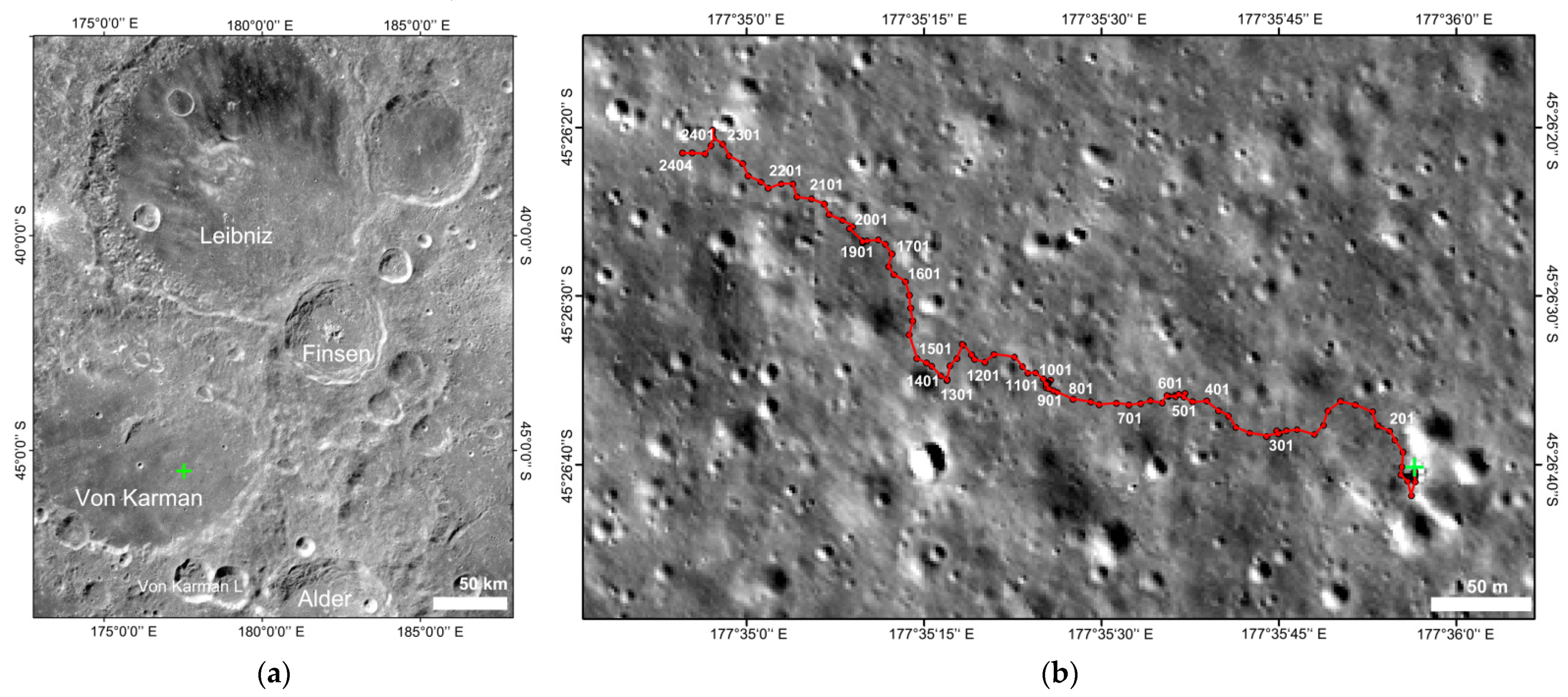
2.1. Geological Context of the CE-4 Landing Site

The Chinese CE-4 spacecraft has successfully landed on the floor of the Von Karman Crater in the South Pole–Aitken basin (SPA; Figure 1a). The SPA is the largest basin discovered in the solar system, and the age is estimated to be 4.2 Ga [30]. The materials from the upper layer of the lunar mantle to the depth of ~100 km might be excavated to the surface, including olivine and low-calcium pyroxene in the SPA [1,31]. The Von Karman crater was formed in the SPA, and the age is dated to ~3.6 Ga [32]. The CE-4 landing site is located on the ejecta ray of the Finsen crater, which contributes an ejecta deposit of ~7 m calculated by the model proposed by Pike et al. [33]. The thickness of the lunar regolith is estimated to be ~12 m by the LPR, which is thicker than that of the CE-3 landing site [2,34,35,36]. The loss tangent of lunar materials is estimated to be ~0.005, which is close to that of typical lunar regolith [2,35]. It shows that the EM attenuation rate at CE-4 is less than that of regolith at the CE-3 landing site [37]. The origin of those regolith developed on the ejecta materials source from nearby craters (e.g., Finsen, Alder, Von Karman L, and L’ [2]).

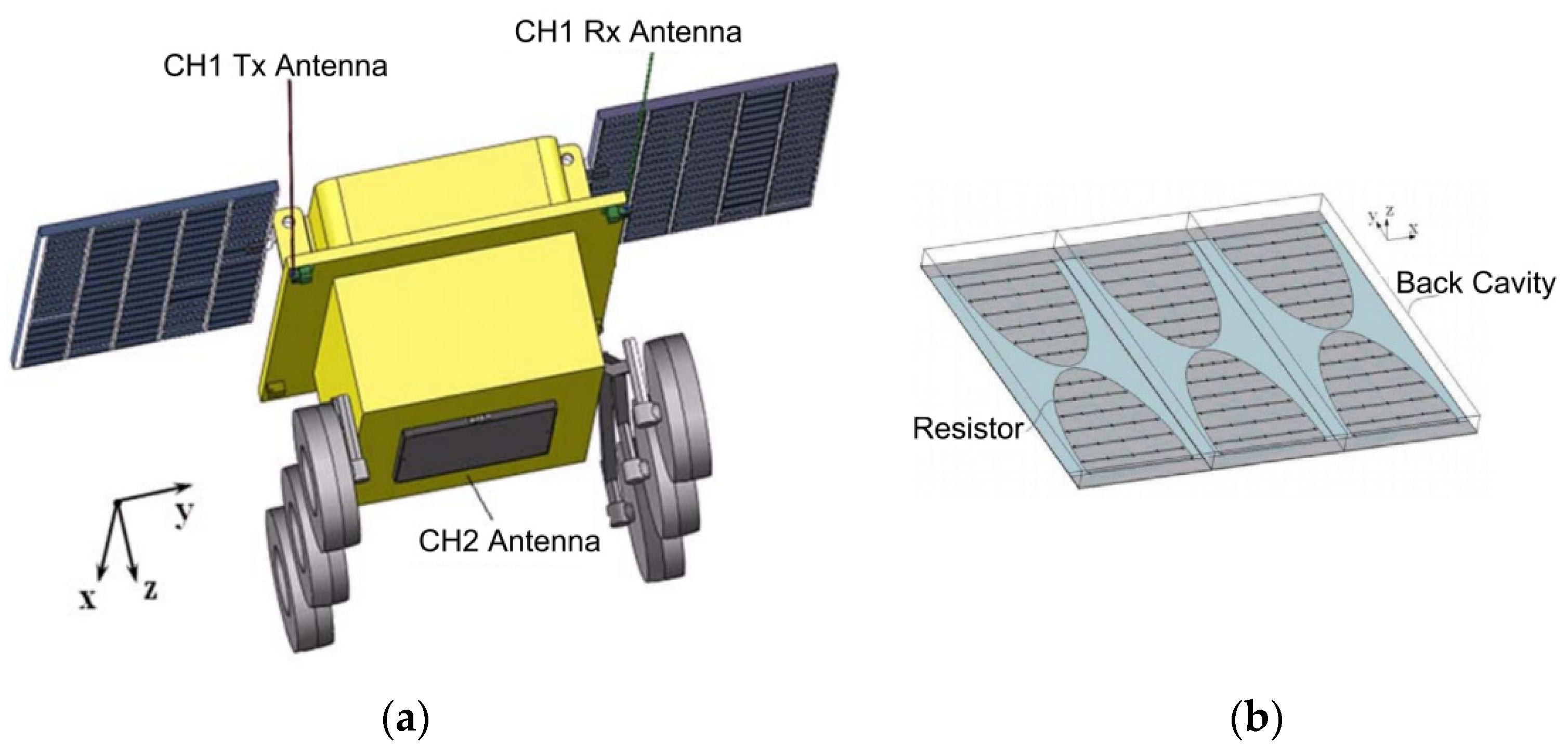
2.2. LPR Data Collections and Processing

The Yutu-2 rover has walked for 589.6 m during the first 24 lunar days (Figure 1b). The LPR obtains 266,073 and 48,282 traces of high-frequency data (antenna 2B) and low-frequency data, respectively. In LPR data collection, 1-bit quantization and non-uniform sampling methods were adopted [21]. A variable gain method is used to compress the strong signals and amplify the weak signals. Besides, to improve the signal-to-noise ratio, each trace of LPR data results from the accumulation of multiple measurements. Thus, it is necessary to pre-process the raw data to recover the actual LPR signal [19].

The flow of data processing of the LPR starts from level 2B data. The processes in this study mainly include trace editing, band-pass filtering, background removal, time delay adjustment, and spherical and exponential compensation (SEC) gain setting [2].

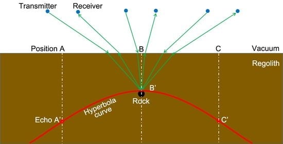
2.3. Traditional Hyperbolic Fitting Method

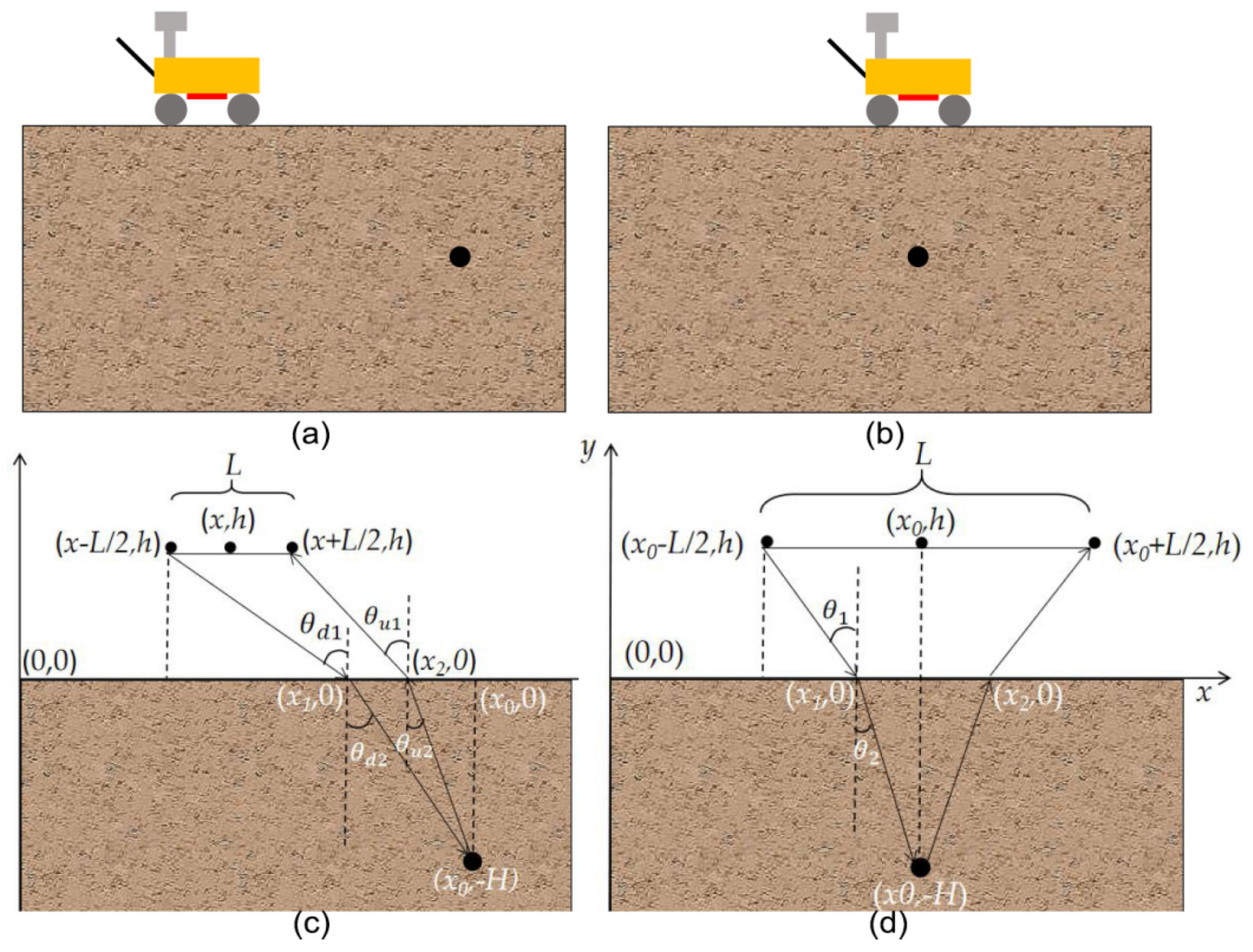
The hyperbola fitting method has been widely used in the GPR field [38]. It is based on the assumption that the depth of reflectors is much greater than the height and spacing of the GPR antenna so that the geometry and position of the antenna can be ignored. The buried reflector within the lunar regolith forms a hyperbola curve in the radar image [38]. The relative permittivity of the lunar regolith above the reflector is closely related to the hyperbolic curve pattern, which can be obtained by the hyperbolic fitting method. The velocity of the LPR radar pulse in the lunar regolith can be described as

$$v=\frac{c}{\sqrt{{\epsilon }_r{\mu }_r}}$$

(1)

where μ_r is the relative permeability of the medium; ε_r is the relative permittivity of the lunar materials; c is the speed of the EM wave in the free space (here we suppose c = 0.3 m/ns). Generally, the relative permeability of the lunar regolith is approximately close to 1 [6], so that Equation (1) can be rewritten as follows

$${\epsilon }_r={\left(\frac{c}{v}\right)}^2$$

(2)

The time delay of the reflected echo can be described as

$$t=\frac{2\sqrt{H^2+{(x-x_0)}^2}}{v}$$

(3)

where (x, 0), (x₀, −H) are the position of the Yutu-2 rover and the reflector (as shown in Figure 2 and Figure 3). The variables t and x can be obtained from the hyperbolic curve in the radar image. H, v, and x₀ can be derived by the hyperbola fitting. Once the v is derived, the relative permittivity of the lunar material can be simply calculated by the Equation (2).

2.4. New Method

The hyperbola fitting method has good performance in the GPR field. However, this is not the case for LPR as shown in Figure 2 and Figure 3. The layout of the LPR antennas is quite special. The transmitting and receiving antennas are allocated at the bottom of the Yutu-2 rover, and it has to be lifted to avoid obstacles while the LPR travels on the lunar surface. The antenna height and spacing are ~0.3 m and 0.16 m, respectively [21]. A new method considering antenna height and spacing is required.

According to Snell’s law, the following equations can be derived.

$$\frac{\sin {\theta }_{d1}}{\sin {\theta }_{d2}}=\frac{\sin {\theta }_{u1}}{\sin {\theta }_{u2}}=\sqrt{\epsilon }$$

(4)

where,${\theta }_{u1}$, ${\theta }_{u2}$, ${\theta }_{d1}$ and ${\theta }_{d2}$ are the incident angle and the refraction angle of the up-going wave and the downward-going wave, respectively. According to the geometric relationship, as shown in Figure 3a,c, the following equations can be derived.

$$\sin {\theta }_{d1}=\frac{\left|x-\frac{L}{2}-x_1\right|}{\sqrt{h^2+{(x-\frac{L}{2}-x_1)}^2}}$$

(5)

$$\sin {\theta }_{d2}=\frac{\left|x_0-x_1\right|}{\sqrt{H^2+{(x_0-x_1)}^2}}$$

(6)

$$\sin {\theta }_{u1}=\frac{\left|x_0-x_2\right|}{\sqrt{H^2+{(x_0-x_2)}^2}}$$

(7)

$$\sin {\theta }_{u2}=\frac{\left|x+\frac{L}{2}-x_2\right|}{\sqrt{h^2+{(x+\frac{L}{2}-x_2)}^2}}$$

(8)

where h and L are the antenna height and antenna spacing, respectively. The position of the echo reflector, the transmitting and receiving antenna are (x₀, −H), (x₀ − L/2, h), (x₀ + L/2,h), respectively. The position of the incident and emission points are (x₁, 0) and (x₂, 0), respectively. Assuming the propagation distances in the free space and lunar material are l₁ and l₂, respectively. Hence, the two-way travel time t can be re-described as

$$t=\frac{l_1}{c}+\frac{l_2}{v}$$

(9)

where l₁ and l₂ can be expressed as

$$l_1=\sqrt{h^2+{(x-\frac{L}{2}-x_1)}^2}+\sqrt{h^2+{(x+\frac{L}{2}-x_2)}^2}$$

(10)

$$l_2=\sqrt{H^2+{(x_0-x_1)}^2}+\sqrt{H^2+{(x_0-x_2)}^2}$$

(11)

Suppose the reflector is horizontally in the middle of the transmitting antenna and the receiving antenna as shown in Figure 3b,d. The incident angle and the refraction angles are θ₁ and θ₂, respectively. The propagation distances of the radar pulse in free space and lunar material are l₀₁ and l₀₂, respectively. t₀ is the time delay of the reflected echo. According to the geometric relationship, the following equations can be derived

$$h\cdot \tan {\theta }_1+H\cdot \tan {\theta }_2=\frac{L}{2}$$

(12)

$$t_0=\frac{l_{01}}{c}+\frac{l_{02}}{v}$$

(13)

$$l_{01}=\frac{2h}{\cos {\theta }_1}$$

(14)

$$l_{02}=\frac{2H}{\cos {\theta }_2}$$

(15)

Suppose θ = θ₂, Equations (12)–(15) can be combined as

$$\frac{h\sqrt{\epsilon }\sin \theta }{\sqrt{1-\epsilon {\sin }^2\theta }}+H\tan \theta =\frac{L}{2}$$

(16)

$$\frac{h}{\sqrt{1-\epsilon {\sin }^2\theta }}+H\frac{\sqrt{\epsilon }}{\cos \theta }=\frac{t_0}{2}c$$

(17)

Combining the Equations (4)–(8), (16)–(17), we can obtain a group of equations as Equation (18). In Equation (18), x₁, x₂, $\epsilon$, H, $\theta$, t₀, and x₀ are unknown variables, x, t, h, L, and c are the known variables. The number of equations is smaller than those of unknown variables. To calculate these equations, we have to obtain at least two unknown variables by other methods to constrain the solution of the above equations.

The hyperbolic echo pattern of the buried object has a symmetrical feature with the peak. Thus, x₀ can be obtained by the hyperbolic fitting method, and t₀ can be obtained by finding the peak of the hyperbola from the radar image. Therefore, the unknown variables that remained are x₁, x₂, $\epsilon$, H, and $\theta$. Equation (18) can be used to calculate these five unknown variables so that relative permittivity can be obtained.

Specifically, as for a certain point (x, t) on the hyperbola curve, once the peak of the corresponding hyperbola curve (x₀, t₀) is determined, one relative permittivity $\epsilon$ can be obtained by combining (x, t), (x₀, t₀), and Equation (18). In other words, one relative permittivity can be derived by one point on the hyperbola curve. For a hyperbola curve on the radar image, the relative permittivity of the new method is the average of all calculated relative permittivities.

$$\{\begin{array}{c}\frac{\left|x-\frac{L}{2}-x_1\right|}{\sqrt{h^2+{(x-\frac{L}{2}-x_1)}^2}}-\sqrt{\epsilon }\frac{\left|x_0-x_1\right|}{\sqrt{H^2+{(x_0-x_1)}^2}}=0\\ \frac{\left|x+\frac{L}{2}-x_2\right|}{\sqrt{h^2+{(x+\frac{L}{2}-x_2)}^2}}-\sqrt{\epsilon }\frac{\left|x_0-x_2\right|}{\sqrt{H^2+{(x_0-x_2)}^2}}=0\\ \frac{\sqrt{h^2+{(x-\frac{L}{2}-x_1)}^2}+\sqrt{h^2+{(x+\frac{L}{2}-x_2)}^2}}{c}+\frac{\sqrt{H^2+{(x_0-x_1)}^2}+\sqrt{H^2+{(x_0-x_2)}^2}}{\frac{c}{\sqrt{\epsilon }}}=t\\ \frac{h\sqrt{\epsilon }\sin \theta }{\sqrt{1-\epsilon {\sin }^2\theta }}+H\tan \theta =\frac{L}{2}\\ \frac{h}{\sqrt{1-\epsilon {\sin }^2\theta }}+H\frac{\sqrt{\epsilon }}{\cos \theta }=\frac{t_0}{2}c\end{array}$$

(18)

2.5. Regolith Modeling and Numerical Simulation

2.5.1. Simplified Modeling

Homogeneous models are the most ideal model, of which the relative permittivity is set to be the same both in the horizontal and the vertical direction (as shown in Figure 4a). Besides, previous studies on the CE-4 landing site and the Apollo sample measurement have indicated that the lunar regolith is not vertically homogeneous, and the relative permittivity increases with the depth. Therefore, we also established the regolith model with the relative permittivity increasing from 2 to 4 (as shown in Figure 4b).

2.5.2. Stochastic Modeling

The interior structure of the lunar regolith is rather complicated, which includes numerous buried rock fragments of different sizes [4,39,40]. The relative permittivity distribution of lunar regolith is not homogeneous, which exists stochastic disturbances in general [4]. In some places, the disturbance is uniform both vertically and horizontally, while in some other places, obvious horizontal disturbance can be seen [9]. Thus, we established two different stochastic models with fewer and more horizontal disturbances, respectively, as shown in Figure 4c,d. Here, we applied the stochastic modeling method to simulate the lunar regolith, which is closer to the real situation according to the statistic [22,41]. Previous works have applied this method both in the GPR and LPR numerical simulations [41,42,43]. In addition to the simulation method, the effectiveness of the new method can also be verified by laboratory experiments.

2.5.3. FDTD Simulation

Once the regolith models are established. The numerical simulation of LPR is performed by using the two-dimensional gprMax software to obtain the simulated radar images [44,45]. The established regolith models include the homogeneous model, relative permittivity linearly increasing model, and the stochastic model. The input source is the Ricker wavelet, and the center frequency is set as 500 MHz, which is the same as that of the high-frequency LPR [21]. The size of the models is set to 12 × 10 m, the grid size is set to 0.01 m, and the time window is 140 ns. The rock is set horizontally in the middle of the model, with the depth ranging from 1 m to 10 m.

3. Results

As shown in Figure 4a–d, to verify the accuracy of the proposed method, we established four types of simulation models, including the homogeneous model, the vertically increasing model, the stochastic model with fewer horizontal disturbances, and the stochastic model with more horizontal disturbances. We calculated the relative permittivity by the traditional hyperbola fitting method and the new method and compared the estimated value with the real value set in the simulation model.

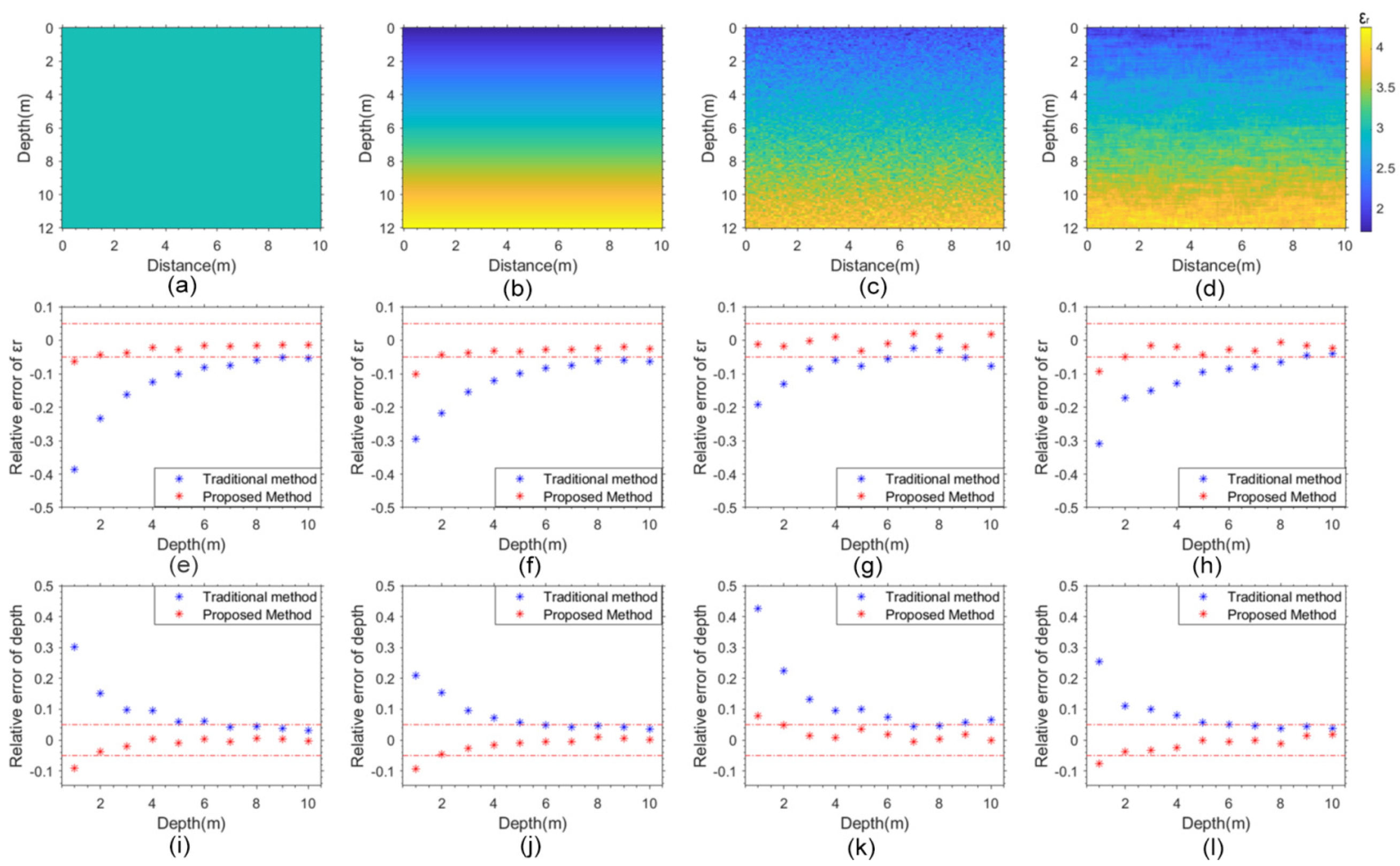
3.1. Numerical Simulation Result

3.1.1. Simulations for Different Models

The estimation results of the simplified models and the stochastic models are shown in Figure 4e–l. Figure 4e–h and 4i–l, respectively show the relative error of the estimated relative permittivity and the depth, respectively. The estimated results show that the accuracy of the traditional method depends on the depth of the reflector (blue dots). The result of the new method (red dots) has less dependency on depth and shows good robustness compared with the hyperbola fitting method. Compared with the results of the simplified models, there exists disturbance in the estimated relative permittivity for the stochastic models.

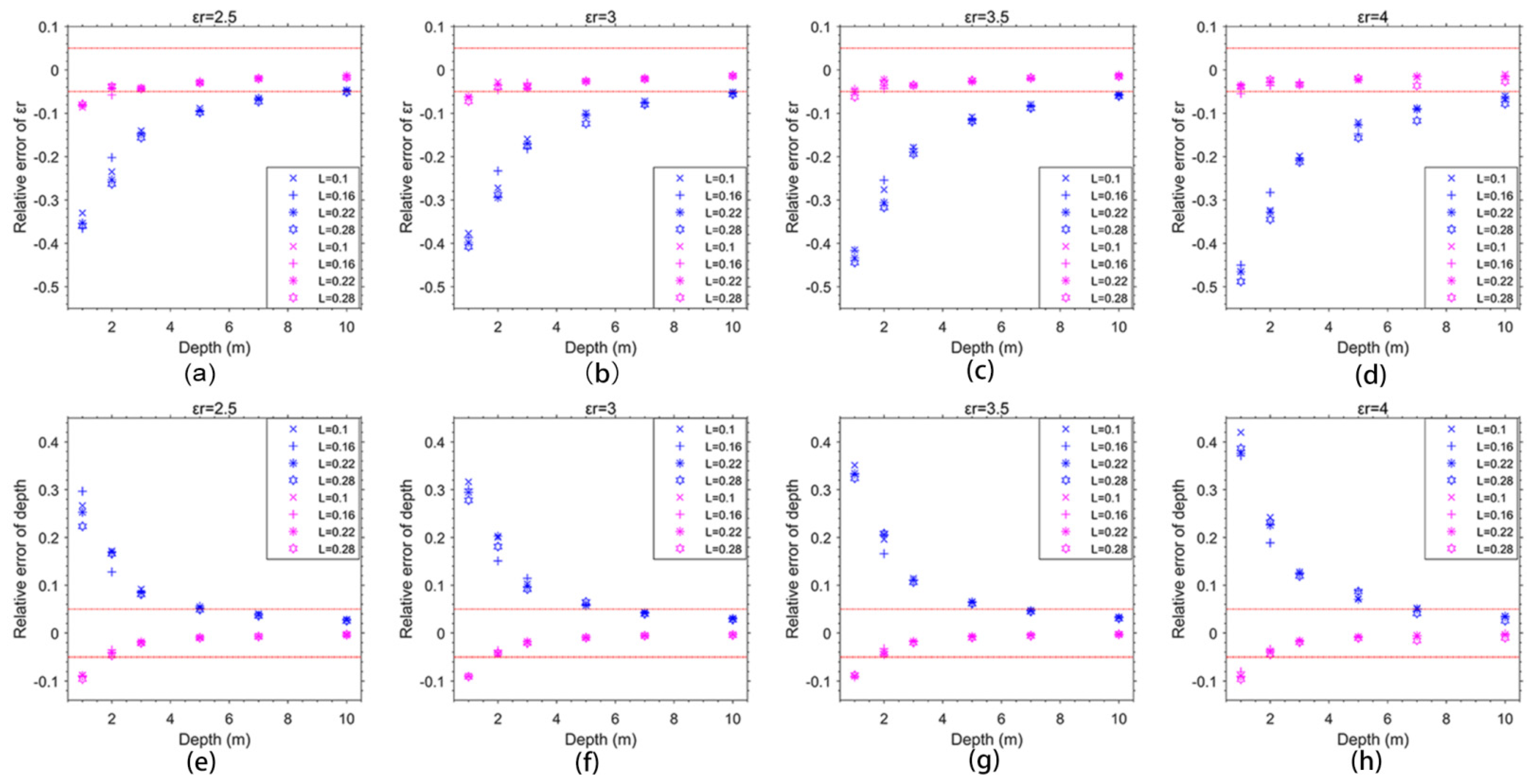
3.1.2. The Influence of Antenna Height and Spacing on Both Methods

The traditional hyperbola fitting method ignores the antenna height and spacing, which causes errors for dielectric constant estimation, especially at the shallow depth. As shown in Figure 4, the estimation accuracy of the hyperbola fitting method increases with the decrease in depth. In particular, the error is intensely upheaved at the shallow depth. To further study the influence of antenna height, we established several homogeneous models with different antenna heights and spacings. The influence of antenna height on the accuracy of both methods is illustrated in Figure 5. The antenna heights are set to be 0.2 m, 0.25 m, 0.3 m, and 0.35 m, respectively. The rock depths are set to be 1 m, 2 m, 3 m, 5 m, 7 m, and 10 m. The results show that the accuracy of the hyperbola fitting method has a significant dependency on the depth of the reflector, especially at the shallow depth. The new method has less dependency on the depth of the reflector compared with the traditional method (Figure 5e–h). Most of the relative errors are within ±5%, and all of the relative errors are within ±10% for the new method. Although subtle discrepancy occurs at a depth less than 2 m for the new method, the results of the new method are barely influenced by the antenna height (red results of Figure 5).

Furthermore, we also considered the influence of antenna spacing on both methods. The various antenna height is set to be 0.1 m, 0.16 m, 0.22 m, and 0.28 m, respectively. The rock depths are set to be 1 m, 2 m, 3 m, 5 m, 7 m, and 10 m. The calculated results are shown in Figure 6a–h. Both the relative error of estimated relative permittivity and depth are analyzed. The results show that the accuracy caused by the antenna spacing has less influence on both methods compared with that of antenna height. The subtle discrepancy can be observed for the hyperbola fitting method at the shallow depth. In conclusion, we can infer that the proposed method is much more robust to calculate the relative permittivity compared with the traditional method.

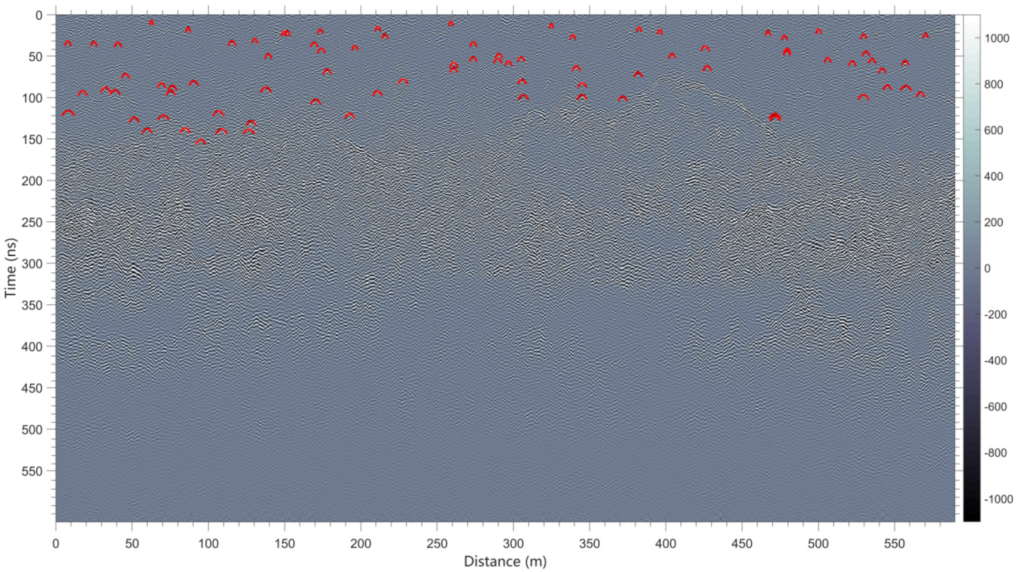
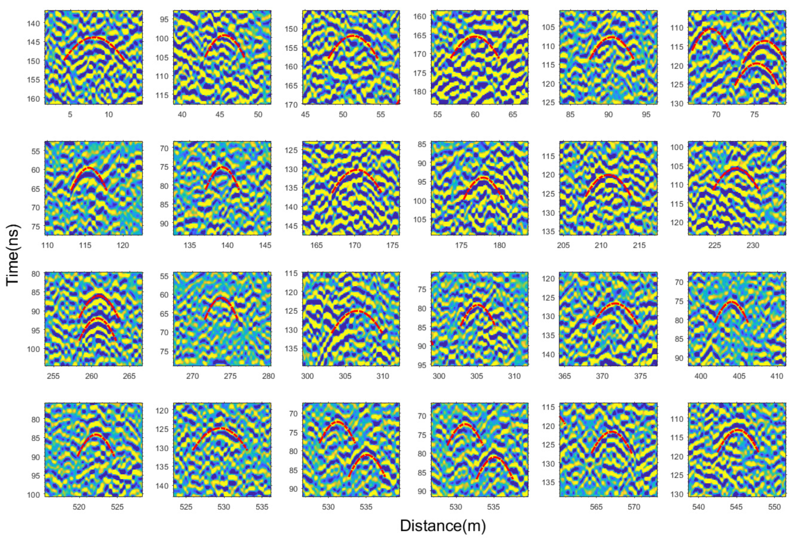
3.2. The high-Frequency LPR Radar Image within the First 24 Lunar Days

Eighty-three hyperbolic echo patterns are recognized in the high-frequency LPR radar image within the first 24 lunar days (red curves in Figure 7). The radar survey distance within the first 24 lunar days is ~589.6 m, and its routine is shown in Figure 1b.

As shown in Figure 7, only obvious hyperbola-like curves are selected in the radar image, and some detailed hyperbola curves are plotted in Figure 8. We applied both the hyperbola fitting method and our proposed method to calculate the relative permittivity. The estimated results are plotted in Figure 9a. The difference of the calculated relative permittivity by the two methods increases with the decrease in depth (Figure 9a), which is consistent with those of the simulation results (Figure 4). The traditional method underestimated the relative permittivity, especially at the shallow depth. Based on the relative permittivity calculated by the proposed method, we obtained an empirical relationship between the relative permittivity and two-way travel time (red line in Figure 9a), expressed as Equation (19).

$$\epsilon =\frac{4.9t+152.9}{t+67.2}$$

(19)

Based on the fitting result, we transformed the two-way travel time versus depth for accurate estimation of the lunar regolith thickness at the CE-4 landing site. As shown in Figure 9b, the blue and red lines represent the depth derived by the relative permittivities that are calculated by the traditional hyperbola fitting method and the proposed method, respectively. The calculated regolith depths are 12 m and 11.1 m, respectively. Therefore, the estimated thickness of the lunar regolith at the CE-4 landing site is improved ~8% compared with that calculated by Li et al. [2].

4. Discussion

4.1. The Comparison of the Traditional and Proposed Method

Both methods use the hyperbola curves to calculate the relative permittivity. The hyperbola fitting method assumes that the antenna height and spacing are zero, and only one equivalent relative permittivity can be obtained for all selected points from a hyperbola curve, which reflects the equivalent dielectric distribution above the reflector. In other words, it can only obtain one relative permittivity from one hyperbola curve. As for the proposed method, the relative permittivity is not derived from the hyperbola curve pattern or curve fitting. Instead, once the position of the peak point of the hyperbola is determined, each point on the hyperbola curve can calculate one relative permittivity according to the geometric relationship. In general, a relative permittivity can be obtained at each picked point on a specific hyperbola curve, the result of the new method is the average of all calculated relative permittivities.

4.2. The Influence of Antenna Height and Antenna Spacing

The hyperbola curve fitting method is based on a simplified model and ignores the antenna height and spacing. The estimation error at the shallow depth caused by the simplified model is more obvious than that at the deep depth. This is mainly because antenna height and spacing are comparable to the reflector depth when the reflector is at the shallow depth, in which case the antenna height and spacing should not be ignored. However, at the deep depth, the depth of the reflector is much smaller than the antenna height and spacing, the influence of the antenna height and spacing on the simplified model of the hyperbola fitting method becomes subtle. As for the proposed method, although subtle discrepancy can be observed at the shallow depth, the estimation accuracy has less dependence on antenna height and spacing.

5. Conclusions

The hyperbola fitting method is based on the simplified model, which ignores the antenna height and spacing. Simulation results show that the influence of antenna height on the traditional method increases with the decrease in depth. The previous works using the hyperbola fitting method have underestimated the relative permittivity of the lunar regolith, especially at the shallow depth. The proposed method has good performance at both shallow and deep depth, and the accuracy is less dependent on the depth of reflectors. We selected eighty-three obvious hyperbola curves in the LPR radar image and calculated the relative permittivity both by the traditional and proposed methods. The result shows that the proposed method improved the calculated relative permittivity at a depth of 0–3 m, 3–6 m, and 6–10 m by 35%, 14%, and 9%, respectively. Finally, the estimated thickness of the lunar regolith at the CE-4 landing site is ~11.1 m by the proposed method, which improved by ~8% compared with that of the traditional method.

References

1. Ip, W.H.; Yan, J.; Li, C.; Ouyang, Z. Preface: The Chang’e-3 lander and rover mission to the Moon. Res. Astron. Astrophys. 2014, 14, 1511–1513. [Google Scholar] [CrossRef]
2. Li, C.; Liu, D.; Liu, B.; Ren, X.; Liu, J.; He, Z.; Zuo, W.; Zeng, X.; Xu, R.; Tan, X.; et al. Chang’E-4 initial spectroscopic identification of lunar far-side mantle-derived materials. Nature 2019, 569, 378. [Google Scholar] [CrossRef]
3. Li, C.; Su, Y.; Pettinelli, E.; Xing, S.; Ding, C.; Liu, J.; Ren, X.; Lauro, S.E.; Soldovieri, F.; Zeng, X.; et al. The Moon’s farside shallow subsurface structure unveiled by Chang’E-4 lunar penetrating radar. Sci. Adv. 2020, 6, 6898. [Google Scholar] [CrossRef] [Green Version]
4. Carrier, W.D.; Olhoeft, G.R.; Mendell, W. Physical properties of the lunar surface. In Lunar Source Book; Heiken, G.D., Vaniman, D.T., French, B.M., Eds.; Cambridge University Press: New York, NY, USA, 1991; pp. 475–594. [Google Scholar]
5. Campbell, B.A.; Hawke, B.R.; Thompson, T.W. Regolith composition and structure in the lunar maria: Results of long-wavelength radar studies. J. Geophys. Res. 1997, 102, 19307–19320. [Google Scholar] [CrossRef]
6. Olhoeft, G.R.; Strangeway, G.D. Dielectric properties of the first 100 meters of the Moon. Earth Planet. Sci. Lett. 1975, 24, 394–404. [Google Scholar] [CrossRef]
7. Ono, T.; Kumamoto, A.; Nakagawa, H.; Yamaguchi, Y.; Oshigami, S.; Yamaji, A.; Kobayashi, T.; Kasahara, Y.; Oya, H. Lunar radar sounder observations of subsurface layers under the nearside maria of the Moon. Science 2009, 323, 909–912. [Google Scholar] [CrossRef] [PubMed] [Green Version]
8. Phillips, R.J.; Adams, G.F.; Brown, W.E.; Eggleton, R.E.; Jackson, P.; Jordan, R.; Linlor, W.J.; Peeples, W.J.; Porcello, L.J.; Ryu, J. Apollo Lunar Sounder Experiment; Technical Report; NASA: Washington, DC, USA, 1973. [Google Scholar]
9. Ding, C.; Li, C.; Xiao, Z.; Su, Y.; Xing, S.; Wang, Y.; Feng, J.; Dai, S.; Xiao, Y.; Yao, M. Layering Structures in the Porous Material Beneath the Chang’e-3 Landing Site. Earth Space Sci. 2020, 7, e2019EA000862. [Google Scholar] [CrossRef]
10. Fa, W.; Zhu, M.; Liu, T.; Jeffrey, B.P. Regolith stratigraphy at the Chang’E-3 landing site as seen by lunar penetrating radar. Geophys. Res. Lett. 2015, 42, 10179–10187. [Google Scholar] [CrossRef]
11. Dong, Z.; Fang, G.; Ji, Y.; Gao, Y.; Wu, C.; Zhang, X. Parameters and structure of lunar regolith in Chang ’ E-3 landing area from lunar penetrating radar ( LPR ) data. Icarus 2017, 282, 40–46. [Google Scholar] [CrossRef]
12. McKay, D.; Heiken, G.; Basu, A.; Blanford, G.; Simon, S.; Reedy, R.; French, B.; Papike, J. The lunar regolith. In Lunar Source-Book; Heiken, G.D., Vaniman, D.T., French, B.M., Eds.; Cambridge University Press: New York, NY, USA, 1991; pp. 285–356. [Google Scholar]
13. Hagfor, T. Backscattering from an undulating surface with application to radar returns from the Moon. Geophys. Res 1964, 97, 13319–13346. [Google Scholar] [CrossRef]
14. Fa, W.; Wieczorek, M.A. Regolith thickness over the lunar nearside: Results from earth-based 70-cm Arecibo radar observations. Icarus 2012, 218, 771–787. [Google Scholar] [CrossRef]
15. Watters, T.R.; Campbell, B.; Carter, L.; Leuschen, C.; Plaut, J.; Picardi, G.; Orosei, R.; Safaeinili, A.; Clifford, S.; Farrell, W.; et al. Radar sounding of the Medusae fossae formation mars: Equatorial ice or dry, low-density deposits? Science 2007, 318, 1125–1128. [Google Scholar] [CrossRef] [PubMed] [Green Version]
16. Orosei, P.; Rossi, A.; Cantini, F.; Graziella. Radar sounding of Lucus Planum, Mars, by MARSIS. Geophys. Res. 2017, 122, 1405–1418. [Google Scholar] [CrossRef] [Green Version]
17. Carter, L.M.; Campbell, B.A.; Holt, J.W.; Phillips, R.; Putzing, N.; Mattei, S.; Seu, R.; Okubo, C.; Egan, A. Dielectric properties of lava flows west of Ascraeus Mons, Mars. Geophys. Res. Lett. 2009, 36, L23204. [Google Scholar] [CrossRef] [Green Version]
18. Porcello, L.J.; Zelenka, J.S.; Adams, G.F.; Jackson, P.L.; Jordan, R.L.; Phillips, R.J.; Brown, W.E.; Ward, S.H. The Apollo lunar sounder radar system. Proc. IEEE 2017, 62, 769–788. [Google Scholar] [CrossRef]
19. Su, Y.; Fang, G.; Feng, J.; Xing, S.; Ji, Y.; Zhou, B.; Gao, Y.; Li, H.; Dai, S.; Xiao, Y.; et al. Data processing and initial results of Chang’e-3 lunar penetrating radar. Res. Astron. Astrophys. 2014, 14, 1623–1632. [Google Scholar] [CrossRef]
20. Jia, Y.; Zou, Y.; Ping, J.; Xue, C.; Yan, J.; Ning, Y. The scientific objectives and payloads of Chang’E-4 mission. Planet. Space Sci. 2018, 162, 207–215. [Google Scholar] [CrossRef]
21. Fang, G.; Zhou, B.; Ji, Y.; Zhang, Q.; Shen, S.; Li, Y.; Guan, H.; Tang, C.; Gao, Y.; Ye, S.; et al. Lunar Penetrating Radar onboard the Chang’e-3 mission. Res. Astron. Astrophys. 2014, 14, 1607–1622. [Google Scholar] [CrossRef]
22. Zhang, L.; Zeng, Z.; Li, J.; Lin, J.; Hu, Y.; Wang, X.; Sun, X. Simulation of the Lunar Regolith and Lunar-Penetrating Radar Data Processing. IEEE J. Sel. Top. Appl. Earth Obs. Remote Sens. 2018, 11, 2. [Google Scholar] [CrossRef]
23. Lai, J.; Xu, Y.; Zhang, X.; Tang, Z. Structural analysis of lunar subsurface with ChangE-3 lunar penetrating radar. Planet. Space Sci. 2016, 120, 96–102. [Google Scholar] [CrossRef]
24. Feng, J.; Su, Y.; Ding, C.; Xing, S.; Dai, S.; Zou, Y. Dielectric properties estimation of the lunar regolith at CE-3 landing site using lunar penetrating radar data. Icarus Int. J. Sol. Syst. Stud. 2017, 284, 424–430. [Google Scholar] [CrossRef]
25. Fa, W. Bulk Density of the Lunar Regolith at the Chang’E-3 Landing Site as Estimated from Lunar Penetrating Radar. Earth Space Sci. 2020, 7, e2019EA000801. [Google Scholar] [CrossRef] [Green Version]
26. Ding, C.; Xiao, Z.; Su, Y.; Cui, J. Hyperbolic reflectors determined from peak echoes of ground penetrating radar. Icarus 2021, 358, 114280. [Google Scholar] [CrossRef]
27. Dong, Z.; Fang, G.; Zhou, B.; Di, Z.; Gao, Y.; Ji, Y. Properties of Lunar Regolith on the Moon’s Farside unveiled by Chang’E Lunar Penetrating Radar. J. Geophys. Res. Planets 2021, 126, e2020JE006564. [Google Scholar] [CrossRef]
28. Ding, C.; Cai, Y.; Xiao, Z.; Su, Y. A rocky hill on the continuous ejecta of Ziwei crater revealed by the Chang’e-3 mission. Earth Planet. Phys. 2020, 4, 1–6. [Google Scholar] [CrossRef]
29. Dong, Z.; Feng, X.; Zhou, H.; Liu, C.; Zeng, Z.; Li, J.; Liang, W. Properties Analysis of Lunar Regolith at Chang’E-4 Landing Site Based on 3D Velocity Spectrum of Lunar Penetrating Radar. Remote Sens. 2020, 12, 629. [Google Scholar] [CrossRef] [Green Version]
30. Hiesinger, H.; Bogert, C.; Pasckert, J.H.; Schmedemann, N.; Robinson, M.S.; Jolliff, B.L.; Petro, N. New Crater Size-Frequency Distribution Measurements of the South Pole-Aitken Basin. In Proceedings of the Lunar and Planetary Science Conference, The Woodlands, TX, USA, 19–23 March 2012. [Google Scholar]
31. Melosh, H.J.; Kendall, J.; Horgan, B.; Johnson, C.B.; Bowling, T. South Pole–Aitken basin ejecta reveal the Moon’s upper mantle. Geology 2017, 45, 1063–1066. [Google Scholar] [CrossRef]
32. Huang, J.; Xiao, Z.; Flahaut, J.; Martinot, M.; Head, J.; Xiao, X.; Xie, M.; Xiao, L. Geological Characteristics of Von Kármán Crater, Northwestern South Pole-Aitken Basin: Chang’E-4 Landing Site Region. J. Geophys. Res. Planets 2018, 123, 1684–1700. [Google Scholar] [CrossRef] [Green Version]
33. Pike, R.J. Depth/diameter relations of fresh lunar craters: Revision from spacecraft data. Geophys. Res. Lett. 1974, 1, 291–294. [Google Scholar] [CrossRef]
34. Xiao, L.; Zhu, P.; Fang, G.; Xiao, Z.; Zou, Y.; Zhao, J.; Zhao, N.; Yuan, Y.; Qiao, L.; Zhang, X.; et al. A young multilayered terrane of the northern Mare Imbrium revealed by Chang’E-3 mission. Science 2015, 347, 1226–1229. [Google Scholar] [CrossRef]
35. Lai, J.; Xu, Y.; Zhang, X.; Yan, L.; Qi, Y.; Xu, M.; Zhou, B.; Dong, Z.; Di, Z. Comparison of Dielectric Properties and Structure of Lunar Regolith at Chang’e-3 and Chang’e-4 Landing Sites Revealed by Ground-Penetrating Radar. Geophys. Res. Lett. 2019, 46, 12783–12793. [Google Scholar] [CrossRef]
36. Xiao, Z.; Ding, C.; Xie, M.; Cai, Y.; Cui, J.; Zhang, K.; Wang, J. Ejecta from the Orientale basin at the Chang’Elanding site. Geophys. Res. Lett. 2021, 48, e2020GL090935. [Google Scholar] [CrossRef]
37. Ding, C.; Xiao, Z.; Wu, B.; Li, Y.; Prieur, N.; Cai, Y.; Su, Y.; Cui, J. Fragments Delivered by Secondary Craters at the Chang’E-4 Landing Site. Geophys. Res. Lett. 2020, 47, e2020GL087361. [Google Scholar] [CrossRef]
38. Daniels, D. Ground Penetrating Radar; The Institution of Electrical Engineers: London, UK, 2004. [Google Scholar]
39. Wilcox, B.B.; Robinson, M.S.; Thomas, P.C.; Hawke, B.R. Constraints on the depth and variability of the lunar regolith. Meteorit. Planet. Sci. 2005, 40, 695–710. [Google Scholar] [CrossRef]
40. Dai, S.; Su, Y.; Xiao, Y.; Feng, J.; Xing, S.; Ding, C. Echo simulation of lunar penetrating radar: Based on a model of inhomogeneous multilayer lunar regolith structure. Res. Astron. Astrophys. 2014, 12, 1642–1653. [Google Scholar] [CrossRef]
41. Ding, C.; Su, Y.; Xing, S.; Dai, S.; Xiao, Y.; Feng, J.; Liu, J.; Li, C. Numerical Simulations of the Lunar Penetrating Radar and Investigations of the Geological Structures of the Lunar Regolith Layer at the CE-3 Landing Site. Int. J. Antennas Propag. 2017, 2017, 3013249. [Google Scholar] [CrossRef]
42. Hu, Y.S.; Zeng, Z.F.; Li, J.; Liu, F. Simulation and processing of LPR onboard the rover of Chang’E-3 mission: Based on multilayer lunar regolith structure stochastic media model. In Proceedings of the International Conference on Ground Penetrating Radar, Hong Kong, China, 13–16 June 2016. [Google Scholar]
43. Jiang, Z.; Zeng, Z.; Liu, F.; Li, W. Simulation and analysis of GPR signal based on stochastic media model with an ellipsoidal autocorrelation function. J. Appl. Geophys. 2013, 99, 91–97. [Google Scholar] [CrossRef]
44. Giannopoulos, A. Modelling ground penetrating radar by GprMax. Constr. Build. Mater 2005, 19, 755–762. [Google Scholar] [CrossRef]
45. Warren, C.; Giannopoulos, A.; Giannakis, I. GprMax: Open source software to simulate electromagnetic wave propagation for ground penetrating radar. Comput. Phys. Commun. 2016, 209, 163–170. [Google Scholar] [CrossRef] [Green Version]
Figure 1. The landing site of the CE-4 and the traveling route of the Yutu-2 rover within the first 24 lunar days. (a) Geological background of the CE-4 landing area. The base map is obtained by Chang’E 2 camera. The image IDs include CE2_GRAS_DOM_07m_J240_38S175E_A, CE2_GRAS_DOM_07m_J201_38S175W_A, CE2_GRAS_DOM_07m_K101_45S175W_A, CE2_GRAS_DOM_07m_K136_45S175E_A. (b) The traveling path of Yutu-2 rover (red line). The base map is obtained by an LRO camera. The image ID is LRO_M1303619844. The green crosses both in (a,b) indicate the CE-4 lander. The red dots mark the navigation points of the rover.
Remotesensing 13 03679 g001
Figure 2. The Yutu2 Rover and the structure of the CH2 Antenna [21]. (a) Schematic diagram of Yutu-2 Rover and the layout of the LPR antenna; (b) structure of the high-frequency antenna.
Remotesensing 13 03679 g002
Figure 3. Schematic diagram of the propagation routine of electromagnetic waves. (a,b) Schematic diagram of Yutu-2 rover, regolith, and rocks. The rock is horizontally far away from the rover in (a) and is horizontally in the middle of the rover in (bd) illustrates the signal propagation routine of (a) and (b), respectively. The antenna height and spacing are L and h, respectively. The red points in (c,d) are the transmitting antenna and the receiving antenna, the blue point is the middle of the antenna, representing the position of the rover.
Remotesensing 13 03679 g003
Figure 4. The established regolith model and simulation results. (ad) Simulation models, representing the homogeneous model, the vertically increasing model, the stochastic model with fewer horizontal disturbances and the stochastic model with more horizontal disturbances; (eh) indicate the calculated relative permittivity by the four models, respectively; (il) represent the derived depth of reflectors in the four models, respectively. The red dash line indicates the error of ±5%. Besides the relative permittivity, the rock depth is another important parameter for geological interpretation, it can be calculated by the two methods and can be used to compare the two methods. Therefore, we showed the estimated rock depth along with the dielectric constant.
Remotesensing 13 03679 g004
Figure 5. The influence of antenna height on the hyperbola fitting method and the proposed method. Blue and red markers indicate the results of the hyperbola fitting method and the proposed method, respectively. (ad) Represent the result of calculated relative permittivity for the simulation models with the relative permittivity of 2.5, 3, 3.5, and 4, respectively. (eh) Represent the results of the calculated depth for the simulation models with the relative permittivity of 2.5, 3, 3.5, and 4, respectively. The two red dash lines indicate the ±5% error.
Remotesensing 13 03679 g005
Figure 6. The influence of antenna spacing on both methods. Blue and red markers indicate the results of the hyperbola fitting method and the proposed method, respectively. (ad) Represent the result of the simulation models with the relative permittivity of 2.5, 3, 3.5, and 4, respectively. (eh) Represent the result of the simulation models with the relative permittivity of 2.5, 3, 3.5, and 4, respectively. The two red dash lines indicate the ±5% error.
Remotesensing 13 03679 g006
Figure 7. The processed high-frequency LPR radar image within the first 24 lunar days. The radar image is obtained based on the level 2B data after bandpass filter (the corresponding filtering parameters are set to 100, 250, 750, 900 MHz, respectively), de-wow, background removal, and SEC gain. The red curves indicate the hyperbola picked in the radar image. The data used for imaging is available on the website http://moon.bao.ac.cn/ (accessed on 10 March 2021).
Remotesensing 13 03679 g007
Figure 8. Several detailed structures of the hyperbola curve observed on the radar image. The red dash curve anchor the profile of the detected hyperbolic echo pattern. Each small region of the radar image is extracted from Figure 7.
Remotesensing 13 03679 g008
Figure 9. The calculated relative permittivities of the lunar regolith and the converted depth. (a). The calculated relative permittivity by the two methods based on the LPR data. The red and blue dot indicates the relative permittivity calculated by the hyperbola fitting method and the proposed method, respectively. The green and maple line represents the fitted result of the relative permittivity estimated by the hyperbola fitting method and the proposed method, respectively. (b) The derived depth by different relative permittivity varies with time delay. The label “Traditional” represents the relative permittivity calculated by Li et al. [2] Constant relative permittivity is used for depth transform. The label Proposed indicates the result of the proposed method.
Remotesensing 13 03679 g009
Publisher’s Note: MDPI stays neutral with regard to jurisdictional claims in published maps and institutional affiliations.