Article

Intercalibration of ASCAT Scatterometer Winds from MetOp-A, -B, and -C, for a Stable Climate Data Record

by
Lucrezia Ricciardulli
* and
Andrew Manaster
Remote Sensing Systems, 444 10th Street, Suite 200, Santa Rosa, CA 95401, USA
*
Author to whom correspondence should be addressed.
Remote Sens. 2021, 13(18), 3678; https://doi.org/10.3390/rs13183678
Submission received: 5 August 2021 / Revised: 31 August 2021 / Accepted: 10 September 2021 / Published: 15 September 2021
(This article belongs to the Special Issue Remote Sensing of Ocean Surface Winds)

Abstract

:
Scatterometers provide very stable ocean vector wind data records. This is because they measure the ratio of backscattered to incident microwave signal over the ocean surface as opposed to an absolute quantity (e.g., emitted microwave signal). They provide an optimal source of observations for building a long ocean vector wind Climate Data Record (CDR). With this objective in mind, observations from different satellite platforms need to be assessed for high absolute accuracy versus a common ground truth and for fine cross-calibration during overlapping periods. Here we describe the methodology for developing a CDR of ocean surface winds from the C-band ASCAT scatterometers onboard MetOp-A, -B, and -C. This methodology is based on the following principles: a common Geophysical Model Function (GMF) and wind algorithm developed at Remote Sensing Systems (RSS) and the use of in situ and satellite winds to cross-calibrate the three scatterometers within the accuracy required for CDRs, about 0.1 m/s at the global monthly scale. Using multiple scatterometers and radiometers for comparison allows for the opportunity to isolate sensors that are drifting or experiencing step-changes as small as 0.05 m/s. We detected and corrected a couple of such changes in the ASCAT-A wind record. The ASCAT winds are now very stable over time and well cross-calibrated with each other. The full C-band wind CDR now covers 2007-present and can be easily extended in the next decade with the launch of the MetOp Second Generation scatterometers.

Graphical Abstract

1. Introduction

The World Meteorological Organization (WMO) Global Climate Observing System (GCOS) identified ocean surface winds as one of the Essential Climate Variables [1]. Changes in the surface wind patterns and intensity affect surface heat and moisture fluxes, impact the redistribution of heat and moisture by shifting convective regions, and affect the transfer of momentum to the ocean circulation. These air-sea interaction mechanisms are important components of the climate system controlled by ocean surface winds. Reliable observational quantification of changes in the wind forcing—and their accurate portrayal in climate models—is a major scientific challenge. On a global scale, wind trends are extremely small and their detection requires highly accurate Climate Data Records (CDRs). This is important for climate research because even if wind trends are small on a global scale, long-term changes in atmospheric circulation (e.g., trade winds and Walker circulation) affect the global hydrological cycle, as they impact precipitation/evaporation over the ocean [2,3].
Space-based observations of ocean surface winds at the global scale have been available for more than 30 years, and efforts to carefully integrate them into stable CDRs are underway at several institutions including RSS, EUMETSAT, The Royal Netherland Meteorological Institute (KNMI), and NASA JPL, with contributions from many investigators from other institutions, as thoroughly described in a collaborative article [4]. Additional details on the CDR development efforts are described in [5,6,7,8,9,10,11].
Starting in 1987 with microwave (MW) radiometers, and in 1991 with a series of scatterometers, satellite sensors provide an opportunity to continuously monitor surface winds with observations homogeneously distributed over the global oceans. Altimeters and Synthetic Aperture Radars also contribute to the space-observations, but their limited swath width and spatial coverage poses some challenges in regards to using them for climate research [12,13,14]. Combining observations from different sensors with the accuracy required for a CDR is a difficult task. The required climate-quality accuracy of 0.1 m/s at monthly global scales defines very stringent conditions on the intercalibration process [1,4]. The scatterometer data records of ocean surface winds are particularly valuable because scatterometers are inherently stable sensors that measure a ratio (backscattered radiation versus transmitted radiation) as compared to measuring an absolute quantity e.g., the emitted MW radiation observed by radiometers.
The Ku-band (13.4 GHz) scatterometer QuikSCAT [15] played a pivotal role at the beginning of the Ocean Vector Wind (OVW) CDR, by offering a “backbone” with a decade of uninterrupted and stable observations from one single sensor between 1999 and 2009. The methodology to develop a Ku-band CDR is described in detail in Ricciardulli and Wentz [7,8].
Later, the launch of three ASCAT C-band (5.3 GHz) scatterometers [16] on the Meteorological Operational satellites, MetOp-A (2006), MetOp-B (2012), and MetOp-C (2018), provided continuity to the timeseries until present day [17]. The ASCAT scatterometers now represent a new OVW CDR “backbone” from 2007 onward and will provide a cross-calibration target when the new C-band scatterometers on MetOp-Second Generation are launched (SCA on MetOp-SG-B, currently planned for 2025) [17,18,19].
Here we describe the approach we followed to verify the stability of these sensors since the beginning of the mission and to bring the consistency of the wind retrievals between the three ASCAT scatterometers to the required climate-quality accuracy. A pivotal aspect in the development of a CDR from different sensors is the use of a consistent methodology and calibration targets. Scatterometers are active instruments at MW frequencies, for which the observable is the backscatter of waves with wavelengths on the order of a few centimeters, which resonate with capillary waves forced by the wind-roughening at the ocean surface [20].
The wind retrievals are typically based on the inversion of the Geophysical Model Function (GMF), an empirical model which describes the dependency of the backscatter on ocean wind speed and direction as well as other parameters related to the viewing geometry (beam incidence angle and polarization state) and ocean conditions (i.e., viscosity or Sea Surface Temperature, SST). The quality of the wind retrievals is therefore highly dependent on how the empirical GMF is developed and calibrated, which is performed by training the observed backscatter response using an optimal ground truth for wind speed and direction. In terms of calibration targets for a given GMF, there are many options as the ground truth can be represented by in situ observations such as ocean buoys or airborne sensors, winds from numerical weather prediction models, wind retrievals from other space-based sensors, or a combination of these. For this reason, different GMFs are developed at different processing centers/institutions with assumptions that better fit their needs, whether it be processing winds for operational purposes in near-real-time, data assimilation, keeping the methodology consistent with previous versions/additional sensors, or using the retrievals to develop a CDR. As a result, satellite wind datasets produced by different processing centers are not entirely consistent at all wind regimes. Additionally, different quality controls (i.e., rain flagging or rain correction, or removal of questionable data) are applied, resulting in additional inconsistencies. Most of the differences among the datasets are small, except at high wind speeds and in areas affected by rain, due to the sparse ground truth measurements and difficulty in calibrating the models at extreme conditions [4,21,22].
The operational EUMETSAT ASCAT scatterometer winds are developed and processed at KNMI, by employing GMFs (CMOD5.n, and more recently CMOD7) trained using Numerical Weather Prediction (NWP) and buoy winds at a reference height of 10 m [23,24,25]. An additional dataset is processed at the NOAA NESDIS Center for Satellite Applications and Research (STAR), which developed a modified GMF (CMOD5.h) to improve retrievals at high winds by training the model using airborne measurements in storms [26,27].
The approach followed at Remote Sensing System (RSS), described here and earlier in [7], is focused on the development of a stable and accurate OVW CDR, starting with the Ku-band QuikSCAT mission, continuing with the C-band ASCAT missions, and later including additional scatterometers at both Ku- and C- frequency bands: ScatSat, ERS, OceanSat, and the future MetOp-SG SCA [4]. The fundamental strategy employed by RSS is to use very similar methodology, calibration ground truth, GMF, wind algorithm, and quality control assumptions for all the sensors included in the CDR. Our approach will be described in detail in the methodology section.
The paper is organized as follows: Section 2 describes the ASCAT datasets which are the focus of our study along with all other datasets used for the calibration and validation of the RSS ASCAT wind retrievals. The methodology is described in Section 3 and Section 4, which focus on the GMF and the calibration adjustments, respectively, both developed for this specific CDR. The next sections describe the results of the validation with buoys and other satellite sensors (Section 5), a study on the rain impact on the retrievals (Section 6), and the quality of the wind retrievals at high winds (Section 7). The manuscript ends with a discussion about the results and future plans (Section 8). A list of acronyms and instruments full names, including their funding agencies, is provided in the Supplementary Material.

2. Datasets

2.1. ASCAT L1B sigma0

The first of the ASCAT scatterometers was launched on the EUMETSAT MetOp-A platform in October 2006 and became fully operational in May 2007. Two follow-up missions, MetOp-B and MetOp-C, were launched in September 2012 and November 2018, respectively. The three satellites, MetOp-A, -B, and -C, carry identical ASCAT instruments, and they are all currently operational, with ASCAT-A approaching its decommissioning phase, which is planned for the end of 2021 [17]. The main objective of ASCAT is the measurement of wind speed and direction over the oceans, though ASCAT is also used for studying polar ice, soil moisture, and vegetation.
ASCAT is a C-band scatterometer with 3 vertically polarized (V-Pol) antennas transmitting pulses at 5.255 GHz. The fan-beam antennas are oriented at 45, 90, and 135 degrees with respect to the satellite track [16]. The antennas extend on either side of the instrument, resulting in a double swath of observations, each about 500 km wide separated by a gap of about 360 km. The Local Time of Ascending Node (LTAN) for the three scatterometers in the nominal and extended phases of the missions has been approximately 9:30 p.m., with a “Trident” orbit configuration to minimize orbital gaps until a recent shift to a “Tristar” configuration since ASCAT-A started a deorbiting phase, which has caused it to shift to an earlier LTAN (Figure 1) [17]. More information on the ASCAT instrument is available from [16,28,29].
The official operational ASCAT wind retrievals (L2B) are processed by KNMI and are distributed by EUMETSAT OSI-SAF via the Earth Observation Portal (https://eoportal.eumetsat.int/, accessed on 15 July 2021) [29].
Here we focus on a different wind product developed by RSS in order to achieve a high degree of consistency with other wind products from the Ku-band scatterometer QuikSCAT and several MW radiometers, as part of a 30+ year CDR of Ocean Surface Winds.
We obtain 12.5 km ASCAT L1B backscatter (σ0) data in NetCDF format (ASCSZR1B files) from the EUMETSAT portal, for the three scatterometers A, B, and C, for the duration of the missions and routinely download the latest orbital files within a couple weeks of the observed times. Campaigns and analyses are regularly performed at EUMETSAT to cross-calibrate these backscatter observations for the three scatterometers within 0.1–0.2 dB and develop a backscatter CDR as described in [30,31,32,33].
The EUMETSAT L1B files contain triplets of backscatter observations for the three beams, organized in 82 Wind Vector Cells (WVC) for each scan, with a total of about 3300 scans per orbit. We reorganize the original L1B data into orbits starting at the South Pole for consistency with the QuikSCAT and other orbital data organization followed at RSS (see https://www.remss.com/missions/ascat/, accessed on 2 August 2021). Each WVC on each beam is characterized by a different Earth incidence angle. The viewing geometry, orbital parameters, and quality flags needed for the wind processing from the original files are included in the reorganized L1B files, and no changes are made to the actual backscatter observations or any of the original ancillary fields.
We used the reorganized L1B files to develop the GMF (RSS C-2015) and currently use them to produce the RSS wind retrievals organized on the original swaths (L2B) or gridded on 25 km global twice-daily maps, for both ascending and descending passes (L3 daily). We additionally produce 3-day, weekly, and monthly composite gridded maps. All these products for the entire missions of the three ASCAT scatterometers and the GMF are freely available at https://www.remss.com/missions/ascat/ (accessed on 2 August 2021), together with an image browser and support material to read the files.

2.2. Moored-Buoy Winds

In situ measurements of ocean surface wind speed collected by a network of moored buoys distributed over the global ocean provide the most accurate verification dataset for satellite wind retrievals. The buoy observations are managed by different institutions and are spread out among different ocean basins. Buoys in the coastal and offshore waters of the continental United States and Canada and the Pacific Ocean around Hawaii are obtained from the U.S. National Data Buoy Center (NDBC) and the Canadian Marine Environmental Data Service (MEDS). In the equatorial ocean regions, observations are made by buoys in the Tropical Atmospheric Ocean (TAO/TRITON) array in the Pacific Ocean [34], the Pilot Research Moored Array in the Tropical Atlantic (PIRATA) in the Atlantic [35], and the Research Moored Array for African–Asian–Australian Monsoon Analysis (RAMA) in the Indian Ocean [36]. These datasets are routinely obtained from the Pacific Marine Environmental Laboratory (PMEL). The wind measurements taken by more than 200 of these buoys are subject to an additional quality control, which addresses issues such as missing or repeated data, blank fields, or out-of-bounds data. The buoy measurements are then converted to 10 m Equivalent Neutral wind using a logarithmic vertical wind profile [37,38], and 10-min observations are averaged into hourly data. The temporal average is a common operation when comparing a point-wise measurement (e.g., buoys) to satellite observations which refer to averages over a footprint (typically 12–50 km), and is needed to help take into account the difference in spatial sampling between the two observational methods [4,39].

2.3. MW Radiometer Winds

Wind speed retrievals from MW radiometers [40] operating from 2007 onward are used for training the model function (Section 3), for validating the wind retrievals (Section 5 and Section 6), and for providing collocated rain rates, which are used in quality control and rain impact studies. The following sun-synchronous radiometers are part of the “evening train” (approximately 6 p.m. LTAN): SSM/I F13, SSMIS F16, F17, F18, WindSat, and SMAP; while the AMSR-E and AMSR-2 are part of the A-train (1:30 p.m.). The best collocations, in time, with the ASCAT scatterometers (9:30 p.m.) are provided by two non-sun-synchronous radiometers on an inclined equatorial orbit, which over time precess through the diurnal cycle: TMI on TRMM and GMI on GPM [41,42,43,44]. The MW radiometers measure the emission of the wind-roughened ocean surface, which, along with a Radiative Transfer Model (RSS RTM V7/V8 [45,46]), can be used to retrieve wind speed. Most wind algorithms are valid only for rain-free environments as the rain signal is difficult to distinguish from the wind-induced emission. Note that WindSat is the only radiometer capable of observing the wind vector due to its polarimetric channels [47]. In addition to wind speed, radiometer observations from different frequency channels in the range 6–37 GHz allow for the simultaneous measurement of rain rate, columnar water vapor, sea surface temperature (SST), and cloud liquid water. SMAP utilizes a lower frequency at L-band (1.4 GHz) and measures salinity and wind speed. Because of SMAP’s low frequency, its wind retrievals are particularly valuable at high winds and are not affected by rain [48]. Specially-trained algorithms for winds in rain have been developed for WindSat, AMSR-E, and AMSR-2 [49,50].

3. The C-2015 GMF

3.1. Ocean Vector Wind CDR Strategy

Our long-term vision for creating consistent observations of OVW from multiple sensors requires that a consistent methodology be applied to processing both Ku-band and C-band scatterometers. This methodology must be valid at a basic level of processing, starting from the GMFs. This involves choosing a common calibration standard (or training wind datasets) for the different GMFs used to process data from scatterometers operating at different frequencies. Our strategy for OVW-CDR retrievals is summarized in Figure 2: a GMF is developed from a large number of σ0 observations at all polarizations and incidence angles, which are matched to “ground truth” or “calibration” wind speeds and directions; if needed, the impact of SST is also modeled in the GMF. For routine processing, the σ0 from the L1B files are then used to invert the GMF and derive the wind speed and direction that correspond to the measured backscatter at any time. The solution for the wind direction is not unique, and an NWP wind field is used to remove the ambiguity among the possible solutions, by choosing the most likely wind direction solution using a Maximum Likelihood Estimation (MLE) method [15]; if SST is part of the GMF, an ancillary SST field is used to define the state of the ocean at the location/time of the scatterometer observations. The output of the wind retrieval algorithm is the retrieved wind vector, and no additional post-hoc or ocean calibration adjustment is applied. This strategy minimizes the risk of instability in the OVW record over time and makes the methodology easily transferrable to past/future sensors or different processing centers. Due to the different ocean response at different frequencies, each type of sensor uses a different GMF, but they share the same GMF calibration choice.

3.2. GMF Development

The basic principles of the C-band ASCAT GMF and wind algorithm follow the methodology which was originally developed for the Ku-band scatterometer QuikSCAT [7,51], while taking into account the different sensor geometry and frequency. Our choice of calibration used in GMF development is based on microwave radiometer winds, calibrated as 10 m Equivalent Neutral winds [37,38]. The major advantages to this calibration choice are that: (1) The radiometers provide 100+ million collocations, uniformly distributed over the globe; using buoys provides a much smaller number of collocations and is limited to few locations in the tropics and along coastlines; (2) radiometer winds are accurate at all wind regimes from 0–40 m/s, as they are based on an ocean emissivity model that is linear in wind speed, and does not saturate at high winds [46]; (3) the radiometer winds are finely tuned to buoy winds in the range 0–15 m/s; (4) they have been continuously available since 1988, and every new sensor is carefully cross-calibrated versus existing ones during their overlapping years; (5) the non-sun-synchronous radiometers TMI (1998–2014) and GMI (2014–present) provide optimal collocations within a narrow time window, due to their precessing Local Time of observation [41,43]; (6) the radiometers simultaneously observe rain rate, which is used for quality control in both calibration and validation activities.
Similar to the Ku-band GMF [7], the C-band GMF is expressed in Equation (1) as a series of N harmonics of the wind direction φR relative to the radar looking angle (azimuth), where the coefficients Ai express the dependence on the wind speed w and the beam incidence angle θ.
σ 0 = f ( w , φ R , θ ) p o l i = 0 N A i ( w , θ ) p o l cos ( i φ i R )
For the GMF development, we first collocated each ASCAT-A σ0 observation (V-Pol only) within 120 min of a TMI or GMI radiometer wind speed and matched them to the NCEP GDAS wind direction interpolated to the time and location of the scatterometer observation. Note that, while the WindSat radiometer provides both wind speed and direction, and it could have been used to train the GMF. We instead opted to use the wind direction from an NWP model for a couple of reasons: radiometer wind direction retrievals at wind speeds below 7 m/s have a large uncertainty because of the small wind direction signal in the surface emissivity [46,47]; WindSat (6 p.m. LTAN) and ASCAT (9:30 p.m.) do not collocate ideally in time.
Any rain contaminated data was excluded with very conservative flags (i.e., no rain in pixel or surrounding areas) at this stage as rain impacts the σ0 and would bias the resulting GMF. The collocations were used to compose histograms of σ0 binned as function of observed wind speed (0.2 m/s bins in the range 0–70 m/s), relative wind direction (2 deg bins, −180 to 180 deg), and incidence angle (2 deg bins, from 27 to 65 deg).
The final C-2015 GMF was developed by performing a harmonic decomposition of these σ0 histograms onto the wind direction from NCEP relative to the azimuth angle for each incidence angle, and each wind speed. For consistency with the QuikSCAT GMF, we chose to truncate the series at N = 5. The harmonic decomposition becomes noisy at regimes/incidence angles for which less collocations are available e.g., very low or very high winds. The final GMF requires some tuning in these cases. We required the Ai coefficients to go smoothly to zero for w = 0. A preliminary version of the GMF (C-2013) was mostly extrapolated at high winds as there were very few high radiometer winds collocated within 2 h in the small developmental dataset used. The ability to closely collocate TMI and GMI winds in time with ASCAT has provided a much larger training set for use in the C-2015 GMF development. Comparisons of the two versions are discussed in [52]. We used a new statistical approach to tune the GMF at high winds rather than by extrapolation. Over time, we have built a database consisting of more than 50 extratropical storms containing very high winds that are mostly rain-free. These storms are observed by QuikSCAT, WindSat, and ASCAT. This collection has allowed us to tune the GMF in such a way as to match the ASCAT wind intensity to the storm wind fields in the database.
Figure 3 displays the non-directional component of the backscatter (A0 coefficients in non-dimensional units, not dB) and the low order coefficients A1 and A2 which include the contribution of upwind and downwind components, expressed as a function of wind speed and incidence angle. Higher order coefficients are displayed in the supplementary Figure S1.

3.3. SST Impact on C-Band Backscatter

Recent studies using physics-based radar backscatter models and comparisons of different scatterometers to other wind datasets (NWP, radiometers) suggest that, at Ku-band, the backscatter σ0 is a function of other physical properties of the ocean surface such as viscosity and SST [53,54,55,56,57]. We explored the SST impact at C-band by using 10 years of ASCAT-A σ0 observations collocated with GMI wind speeds, NCEP wind directions, and SST from the Reynolds OISST dataset [58] interpolated to the ASCAT time/location. We then performed the harmonic analysis described above, but separately for each incidence angle interval and each SST 3 °C bin.
Figure 4 displays the non-directional GMF coefficient A0 for C-band as a function of wind speed for every SST bin, for a sample incidence angle. The spread of the A0 curves for different SSTs is extremely small, which indicates that the SST-impact at C-band is, definitely, negligible, and therefore, we do not include it in the final version of the GMF C-2015.

3.4. ASCAT-A, -B, and -C Wind Retrievals

A preliminary version of the GMF (C-2013) had been used to process the first version of RSS ASCAT-A winds in 2013 (V1.2). C-2015 has been used since 2016, and the entire mission was reprocessed as version V2.1. At that time, our analyses of ASCAT-A V1.2 suggested the global wind average timeseries dropped by about 0.1 m/s in October 2014 compared to other radiometers/scatterometers [8]. Additional studies confirmed our calibration step-change estimate [59,60]. A correction is not included in the original backscatter from the EUMESAT L1B files. However, EUMETSAT confirmed our calibration jump estimate, and recommended to adjust the σ0 by +0.08 dB for climate accuracy (personal communication). The RSS ASCAT V2.1 winds include such an adjustment starting from October 2014 until present.
The same GMF (C-2015) has recently been used to process data from the newer ASCAT scatterometers on MetOp-B, and -C with the same wind algorithm (V2.1), for the entire duration of each mission. A small update to ASCAT-A (V.2.1.1) was recently processed to correct small calibration issues experienced after 2016 and is described in the Section 4. Figure 5 illustrates the vector wind fields for ASCAT-A, B, and -C for a sample day, 31 December 2020. A large extratropical storm is seen in the Northern Pacific, much larger than the scatterometers’ swath width. The combination of three near-simultaneous views from the three scatterometers provides a complete view of large storms.
Unlike QuikSCAT, ASCAT observations are taken at a wide range of incidence angles. Climate-quality data records require the wind retrievals to be highly accurate at all incidence angles. Figure 6 illustrates the wind Probability Distribution Functions (PDFs) of ASCAT-A wind speeds (solid lines) for a sample year (2016) stratified by Wind Vector Cell (WVC) as displayed by different colored lines, for winds speeds from 0–20 m/s (linear scale), and separately for higher wind regimes (log-scale). Additionally displayed are the PDFs for collocated GMI wind speeds (dashed lines), also stratified by the ASCAT-A WVC. These curves overlap at all WVC without any additional adjustment, suggesting that the ASCAT wind retrievals do not depend on the WVC position, at all wind regimes, confirming a well-designed GMF at all regimes and incidence angles.

4. Fine Calibration Adjustments for Climate-Quality Accuracy

After processing the three ASCATs as V2.1, we performed a careful analysis of their cross-calibration, at global yearly, monthly, daily, and hourly scales, in order to properly estimate and possibly diagnose the reasons for any calibration instabilities. Some small but non-negligible instabilities were found for ASCAT-A. Figure 7 illustrates the calibration analysis where we compared ASCAT-B to the other ASCATs (-A and -C) and to stable radiometer wind datasets from GMI, WindSat, and AMSR-2, for global (55S-55N) monthly collocated averages from 2013 until present. This analysis proved that after the first 6-months of the mission, ASCAT-B has been extremely stable and therefore can be considered as a calibration target for all other sensors. Similarly, after the first 6-months, ASCAT-C has been extremely stable, with just a small bias of 0.05 m/s compared to ASCAT-B. On the other hand, ASCAT-A V2.1 (dashed red curve) experienced two step-changes: one in mid-2016 and a second (accidental) one at the end of 2019 followed by a small drift.
We investigated these step-changes/drifts. It was found that the +0.08 dB correction (see Section 3.4) on ASCAT-A σ0 was accidentally turned off when the code was adapted to process ASCAT-B and -C in October 2019. This is what caused the artificial ASCAT-A V2.1 calibration step-decrease in 2019. The calibration step-increase seen in 2016 is illustrated in more detail in Figure 8, which shows the daily global average differences between collocated V2.1 ASCAT-A and ASCAT-B in 2016, separately, for ascending and descending passes. The jump appeared on Julian day = 204 (22 July 2016), immediately after some missing ASCAT-A orbits on that day. According to KNMI mission log for 2016: “the ASCAT-A winds have been unavailable on 22 July between 0:21 and 10:11 UTC sensing time due to a spacecraft anomaly” (see https://scatterometer.knmi.nl/ascat_osi_25_prod/#modifications, accessed on 12 July 2021). We concluded that this calibration jump is real. We therefore reprocessed all ASCAT-A since the beginning of 2016 and applied an adjustment of −0.05 dB to the σ0 from the L1B files starting on 22 July 2016, and restored the +0.08 dB adjustment which was accidentally turned off in October 2019. The new adjusted version is referred to as ASCAT-A V2.1.1, and its cross-calibration with ASCAT-B is displayed in Figure 7 (solid red curve). A very small residual jump of about 0.02 m/s in the timeseries of the differences between -B and -A is apparent in mid-2017, but at this time we consider it too small to justify any correction. The small drift after 2019 is still visible, and it is still under investigation. No additional adjustment or post-hoc corrections are applied to ASCAT-A or the other two ASCAT scatterometers.
The cross-calibration of the three ASCATs, for rain-free wind retrievals, collocated within 60 min during the overlapping years 2019–2020, is displayed Figure 9. The bias between ASCAT-B and -A is 0.03 m/s, much smaller than the 0.1 m/s accuracy requirement for a CDR, with a standard deviation of 0.5 m/s. The bias for ASCAT-C versus -A and -B is slightly larger in magnitude with -C being systematically lower than the other two sensors by about 0.06–0.08 m/s in 2020. At this time, we did not apply any adjustment to ASCAT-C, but we might revisit this decision after ASCAT-A is decommissioned, and possibly reprocess it.

5. Validation of ASCAT Wind Speed and Direction

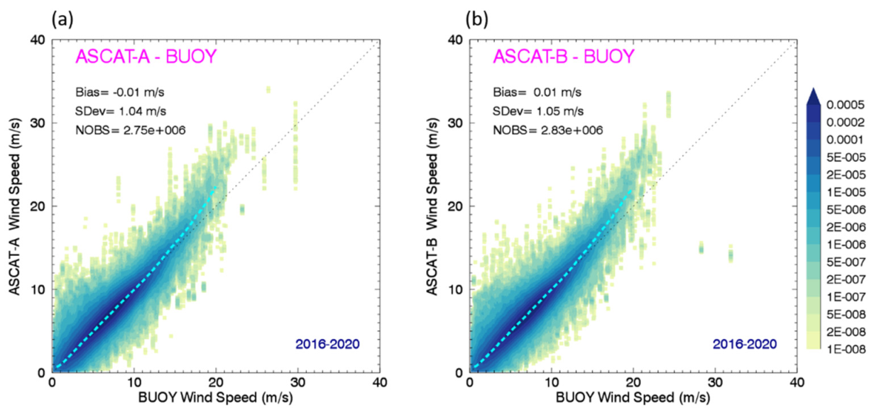
5.1. Validation of Low to Moderate Wind Speeds Using Buoys

Surface ocean winds from the network of global buoys described in Section 2.2 provide an independent verification dataset for the absolute calibration of the ASCAT scatterometers. Note that the buoys have not been used in the development of the GMF or the wind retrievals algorithm. As the in situ measurements are sparse, a large sample needs to be considered in order to verify the calibration in a wide wind speed range. Figure 10 displays the joint PDFs for ASCAT-A and -B collocated within 30 min and a radius of 25 km from the actual buoy location at a given time, as they occasionally move from their nominal location, during the period 2016–2020. Both scatterometers are unbiased with respect to the buoy wind speeds in the range 0–15 m/s. A small bias appears at higher wind speeds as the buoys become less reliable in very rough ocean conditions. The standard deviation between ASCAT and the buoy measurements is of the order of 1 m/s, with an uncertainty approximately equally shared between the two types of instruments. Note that the Standard Deviation for comparisons between ASCATs is of the order of 0.5 m/s (Figure 9).
A finer verification of the absolute calibration is achieved by collecting a set of quadruple collocations: ASCAT-B (swath data L2B) is first collocated with the buoys within 30 min and 25 km; then, for a more time-efficient search, this selection is collocated with ASCAT-A measurements from the gridded dataset (L3), and within 60 min, to ensure an overlap between the two scatterometers (see Figure 1 for the LTAN). Finally, NCEP GDAS winds are interpolated to the ASCAT-B time and location. The wind speed PDFs for this set of quadruple collocations for the year 2016 are displayed in Figure 11a. There is excellent alignment between the ASCAT and the buoy wind PDFs. The alignment is due to the accurate GMF (the PDFs have not been aligned by any post-hoc adjustment to the wind retrievals). The NWP wind PDFs are narrower and slightly shifted towards lower winds. This is because these PDFs are built by interpolating the lower spatial and temporal resolution NWP, in this case the NCEP GDAS 1 deg, 6-hourly wind fields, to the ASCAT-B location. Similarly, in Figure 11b, the wind speed PDFs for quintuple collocations in 2020 are displayed, which additionally include ASCAT-C. The statistics for the collocated data for 2016 and 2020 are summarized in Table 1. The alignments between the buoys and the three ASCATs is still very good, but slightly degraded compared to Figure 11a. This is likely due to noise affecting the much smaller collocation sample in 2020 (2681 quintuple collocations in 2020 versus 74,036 quadruple ones in 2016).
The multiple collocation sets can be used to extract the error for each single dataset [61,62,63]. For a set of triple collocations (e.g., i, j, k = ASCAT, buoys, and NCEP), if we assume that the errors of the datasets are independent from each other, we can calculate the standard deviation σi of each dataset i (e.g., ASCAT) from the standard deviations of the three pairs of differences (e.g., ij = ASCAT-buoy, ik = ASCAT-NCEP, and jk = buoy-NCEP), as described in Equation (2). Using the values in Table 1a, for ASCAT-B, buoys, and NCEP in 2016, we obtain uncertainties (standard deviations) of 0.47, 0.77, and 1.00 m/s, respectively. Using this method, for ASCAT-A we obtain a slightly larger uncertainty of 0.56 m/s.
σ i 2 = ½   ( σ i j 2 + σ i k 2 σ j k 2 )

5.2. Wind Direction

Figure 12 provides an estimate of the uncertainty in the ASCAT retrievals’ wind direction. The figure displays the wind direction root-mean-square (RMS) difference between ASCAT-A or -B and wind measurements from the buoys, collocated within 30 min during the years 2016 to 2020. The RMS difference is a function of wind speed, with wind direction RMS differences being higher at lower wind speeds. This is because the backscatter for a smooth surface (i.e., regions of low winds) is low, which leads to higher uncertainty in the wind direction retrievals. At wind speeds above 7 m/s, the directional RMS compared to buoys is 15 degrees or less. This results from the combination of the uncertainty of the scatterometers’ and the buoy anemometer wind direction measurements. When compared to the NCEP model, the ASCAT RMS at winds above 7 m/s is reduced to about 10 degrees. This is possibly due to the fact that the NCEP model assimilates the ASCAT retrievals, though not this specific dataset. On the other hand, wind direction from a point-source instrument such as the buoy anemometer is expected to present larger differences with those from space-based observations. Larger differences are also observed when the buoy wind direction is compared to those from the NCEP model, interpolated to the buoys’ location and time.

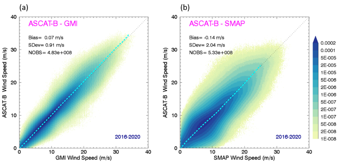
5.3. High Wind Speed Validation Using Radiometers
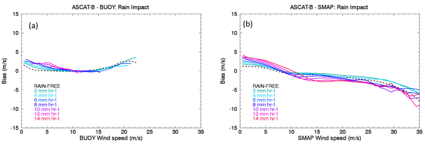
An additional validation source valuable at high wind speeds above 15 m/s, which are less sampled by the buoys, is provided by the radiometers. Figure 13 illustrates the joint PDFs for ASCAT-B collocated within 90 min of the GMI radiometer, and within 240 min of SMAP (due to the LTAN mismatch with ASCAT), for rain-free wind retrievals over 2016–2020. Similar results were found for analyses using ASCAT-A and -C (not shown). The SMAP radiometer winds have been extensively validated versus oil platform anemometers, in situ airborne measurements, and Best-Track estimates in Tropical Cyclones, and verified versus hurricane forecast model wind fields [21,48,49,50]. The ASCAT retrievals are remarkably unbiased versus these radiometers for high wind speeds, up to 35 m/s. Notice that the ASCAT versus GMI winds present a smaller bias (0.07 m/s) and standard deviation (0.91 m/s) compared to SMAP. This is only partially due to the shorter time-collocation window allowed by GMI (90-min). As discussed in Section 2.3, the SMAP radiometer is ideally suited for high wind observations, but due to the lower frequency of operation (L-band), it is less accurate and noisier than other radiometers operating at higher frequencies (such as GMI), particularly at winds below 10 m/s.

6. Rain Impact

Rain can affect the consistency of wind retrievals obtained from scatterometers operating at different frequencies: it affects both direct and backscattered signals due to backscatter from the rain drops (positive wind bias at low winds) and atmospheric attenuation (negative bias at high winds). Additionally, rain can alter the ocean surface roughness via a “splash” effect (small positive bias at low winds), and can cause an artificial rotation of the retrieved wind vectors [22,64]. The impact of rain on wind measurements is proportional to the rain intensity, and is more relevant for sensors operating at higher frequencies. We studied its impact by comparing winds in rain from the C-band ASCAT scatterometers to wind measurements from buoys and the SMAP radiometer, which are either unaffected or minimally affected by rain. Previous studies documented the rain impact for different frequency bands, using comparisons with NWP and buoy measurements. The studies found the rain impact to be minor at C-band [65,66,67], significant at Ku-band [7,68,69] especially at low winds, and negligible at L-band [8,48,63].
The biases between the wind retrievals and the selected validation datasets were stratified according to the rain rate measured using collocated radiometers. Buoys provide a short collocation window of 30 min, but have a relatively small sample size, while SMAP has a relatively large sample size, but is collocated within a larger time frame of 4 h. These collocations were paired with the closest possible rain observation, within 120 min when GMI was available and 4 h when other radiometers were used. A large collocation window for rain rate retrievals is not ideal as rain varies a lot over short time and spatial scales. However, due to the ASCAT LTAN, it is challenging to restrict the collocation window without significantly reducing the number of observations that can be collocated with radiometers, which for a narrow window would mostly include high latitude observations. Our choice of a large collocation window allows for a very large sample of collocations spanning all latitudes and results in less noisy bias curves. With this choice in mind, the rain impact presented here needs to be interpreted in a statistical sense.
Figure 14 illustrates the wind bias between ASCAT-B versus buoys and SMAP winds as a function of wind speed and rain rate (colored lines). The bias for rain-free wind retrievals (black dashed line) is also displayed for comparison to help quantify the rain impact. There are very few observations from buoys above 15 m/s, and the rain impact at high winds is hard to quantify. On the other hand, SMAP provides plenty of observations for the statistics to be accurate up to 35 m/s. The statistics here refer to collocations from 2016 to 2020, for wind bins of 0.1 m/s with at least 10 observations. The relative impact of rain is minimal at high winds (within 10% error), while at very low winds the bias relative to rain-free observations can be significant (1–3 m/s systematic positive bias, up to 100% error) at moderate (4–8 mm/h) to intense rain rates (above 8 mm/h). The impact of rain is also seen in the standard deviation (Supplementary Figure S3), with an increase of about 40–50% in heavy rain (8 mm/h and above) at all wind speeds. At wind speeds of 5–10 m/s the standard deviation is below 2 m/s for rain-free retrievals and about 2.7 m/s in heavy rain. At 20 m/s, the standard deviation is about 3 m/s for rain-free retrievals, reaching about 4 m/s in heavy rain.
In summary, when compared to the impact at other frequency bands, rain droplets’ attenuation and backscatter have very small effects at L-band, but they become relevant at C-band for low winds, and are very significant at Ku-band for both low and high winds.

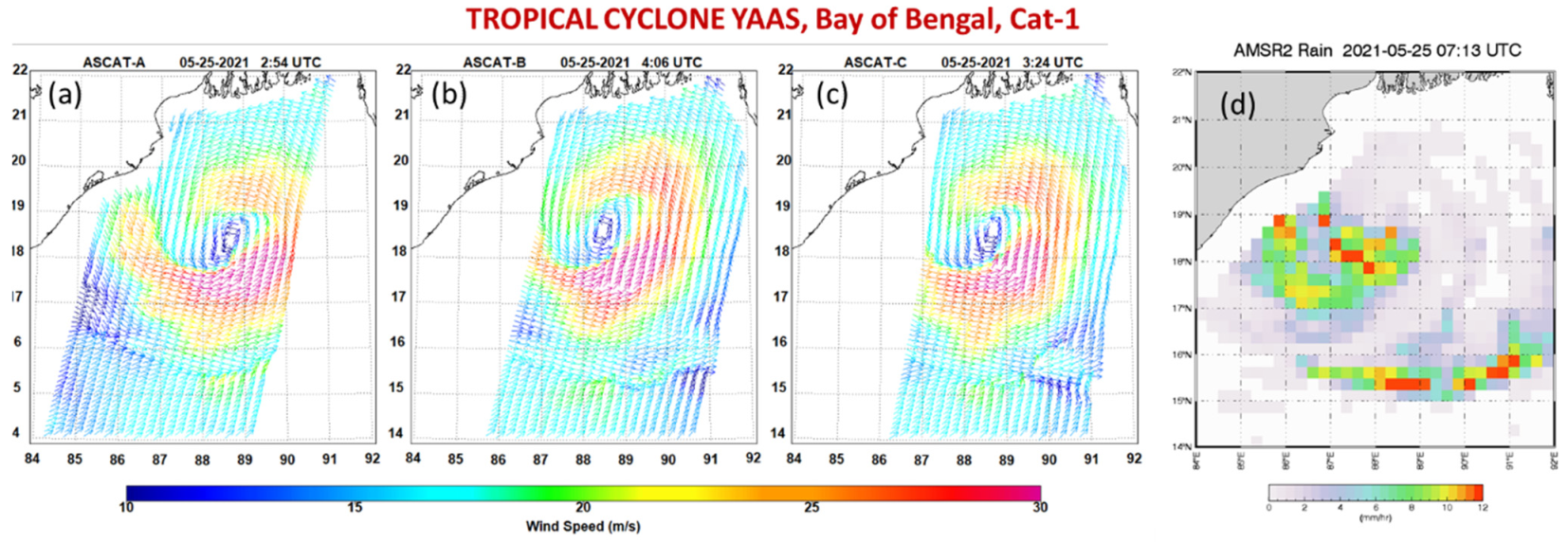
7. Example: ASCAT Wind Retrievals in Tropical Cyclones (TCs)

The analyses presented in the previous sections suggest that the ASCAT wind retrievals are accurate at high winds, up to 35 m/s, even in storms, with relatively small degradation in the presence of intense rain. Figure 15a–c presents an example of the wind vector fields as seen by the ASCAT-A, -B, and -C scatterometers for Tropical Cyclone Yaas, in the Bay of Bengal on 25 May 2021 (descending passes), the day before landfall at an intensity equivalent to Category 1.
The combination of the three scatterometers provides a consistent and complete view of the ocean surface wind field for this tropical cyclone at 3–4 AM (UTC), which is not fully covered by the swath of just a single scatterometer: the eye of the storm is clearly visible in each of the three scatterometers, and the structure of the wind fields are very consistent within the observed time range, with highest winds located in the SE quadrant. The maximum winds at the ASCAT spatial scales (determined from L2B swath files, 12.5 km WVC) were consistent within a 5% margin: 35.4, 36.5, and 35.0 m/s for -A, -B, and -C, respectively. South of the storm, a narrow (frontal) region of convergence is clearly visible and consistent in all three scenes.
Rain rates as observed by AMSR-2 on 25 May 2021, at 0713 UTC, a few hours after the ASCAT passes, are also displayed in Figure 15d. Notice the presence of a rain band at the bottom, which corresponds to the area where the three ASCAT scatterometers consistently display the narrow band of convergence. A small area of divergence at the Eastern edge is also seen in ASCAT-C. Most of these small-scale wind features are likely real and often missed by NWP models [65,66] but there is the possibility of artifacts in some small areas under intense rain [70,71]. An in-depth analysis of closely collocated rain measurements for several views of ASCAT wind fields in storms can shed light into spurious versus real wind variability in convective areas and will be addressed in a future manuscript.
Overall, the wind fields in Figure 15 do not seem affected by rain. A rain impact on the scatterometer winds would appear as an area with spuriously lower/rotated winds in the regions affected by rain. This is not the case here, as there is no apparent attenuation or artificial rotation of the wind direction vectors (typically perpendicular to the spacecraft orbiting direction) even in regions of intense rain. The consistent wind fields and smooth wind direction retrievals in Figure 15 confirm that the three ASCAT scatterometers generally provide reliable observations in Tropical Cyclones for wind speeds, at least up to the Category 1 threshold (33 m/s) [26,48,49,72]. For this specific day, the ASCAT maximum winds (~35–36 m/s, ~68–70 kt) displayed in Figure 15 are within the range of estimates from the SATCON dataset [73] at the same time (~60 kt ± 20 kt), which includes Best-Track data, Dvorak technique, and satellite-based estimates (http://tropic.ssec.wisc.edu/real-time/satcon/202102B.html, accessed on 26 August 2021).
On the other hand, Ku-band scatterometers are less reliable in moderate to intense rain, and the wind direction vectors are distorted by the rain signal affecting the backscatter from the ocean surface [7,22,65]. Above Category 1, the signal from the ASCAT scatterometers starts saturating, and the forward and backscattered radar signal can potentially be attenuated by intense rain. The combination of these effects often caps the ASCAT wind retrievals to about 42 m/s. Examples of intense ASCAT wind retrievals in tropical and extratropical cyclones and signal saturation at high winds are shown in [48,49].

8. Summary and Conclusions

Scatterometers have been providing accurate measurements of ocean vector winds (OVW) for three decades. Here we document our efforts at RSS in making these observations consistent across different sensors, with different operating frequencies and viewing geometry, and meeting stringent accuracy requirements such that they can be combined into a CDR. The efforts described here focus on developing a “C-band backbone” for the CDR covering the years 2007 to present with retrievals from the ASCAT scatterometers on MetOp-A, -B, and -C, launched in 2006, 2012, and 2018, respectively, all currently operational. The strategy described here builds on the development of a “Ku-band backbone” from QuikSCAT measurements taken from 1999–2009, described in [7]. The objective of climate-quality retrievals from different instruments is to achieve stability and consistency over time within 0.1 m/s (in a globally averaged statistical sense). Similar efforts are in progress at the Royal Netherland Meteorological Institute (KNMI) [10], EUMETSAT, NASA Jet Propulsion Laboratory (JPL) [11], and other institutions [4]. The progress of each group, efforts to include additional sensors to the CDR, and coordinated intercomparisons are planned within the CDR working group for the International Ocean Vector Wind Science Team (IOVWST) [https://mdc.coaps.fsu.edu/scatterometry/meeting/past.php, accessed on 10 July 2021].
The wind retrievals at Ku- and -C band described here are based on GMFs that relate the observed radar backscatter to the wind speed and direction from the wind-induced ocean surface roughness. The C-band GMF C-2015 development follows a similar methodology and calibration target as the Ku-band GMF (Ku-2011/KuSST, [7,57]) and is described in detail in this paper. Both GMFs are built around a pivotal choice for calibration target based on wind speed from microwave (MW) radiometers. This aspect is extensively discussed in Section 3. While in situ data from ocean moored buoys are considered the ultimate ground truth for the satellite retrievals to be compared to, here we use them as an independent verification source, rather than a calibration source for developing the GMFs. Buoy winds are ideal for absolute calibration of large samples of wind retrievals, but they are challenging to use for the GMF development due to the relative scarcity of observations.
The C-band GMF was originally developed in 2015, and it has been used to process the wind retrievals for ASCAT-A, -B, and -C for the entire duration of each mission, as V2.1. After examining the cross-calibration among the three scatterometers, and the absolute calibration at all wind speed ranges using buoy data and MW radiometers, an update to the GMF was not deemed necessary. The accuracy of the retrievals for the three scatterometers is still valid at all wind regimes 0-35 m/s, and for all incidence angles. The L2B (swath) and L3 (gridded) datasets along with the GMF C-2015 are available to the public at www.remss.com/missions/ascat (accessed on 2 August 2021). The same GMF, or a preliminary version C-2013, has been used by other institutions to fine tune their model or as a test [24].
To verify the stability of the three ASCAT measurements over time, we constructed globally averaged timeseries from the wind speed differences between ASCAT-B and -A or -C, closely collocated in time. A couple of instabilities/small step-changes were detected in the ASCAT-B minus -A timeseries. Identifying the source of these very small instabilities (<0.1 m/s) in the ASCAT timeseries using buoys is not feasible due to the scarcity of buoy observations, the non-uniformity of the buoy array distribution over the ocean, and frequent interruptions of buoy data due to service on the buoys. For this purpose, we instead used the average wind speed differences versus collocated radiometers (GMI, WindSat, and AMSR-2). We showed that having multiple radiometers available as independent comparison gives the opportunity to isolate which of the ASCAT scatterometers are drifting or experiencing jumps as small as 0.05 m/s (~0.05 dB), if not smaller. It was found that ASCAT-A wind retrievals suffered a small calibration jump of about 0.05 m/s on 22 July 2016, following a spacecraft anomaly. We adjusted the ASCAT-A backscatter measurements by −0.05 dB starting on this day, restored an additional calibration adjustment of +0.08 dB applied since October 2014, which was accidentally turned off in October 2019, and reprocessed ASCAT-A as V2.1.1.
The WMO GCOS accuracy requirement for an ocean wind CDR is 0.5 m/s for low to moderate winds and 10% for winds exceeding 20 m/s. The stability requirement at global scales is 0.1 m/s/decade [1]. Our study showed that the bias between ASCAT-B and -A and versus the buoys is 0.03 m/s or less, much smaller than the 0.1 m/s accuracy requirement for a CDR. The ASCAT wind standard deviation is about 0.5 m/s for low to moderate winds, and about 10% for very high winds, therefore meeting all the CDR requirements. ASCAT-C is consistently lower than ASCAT-B and -A by about 0.06–0.08 m/s, but the timeseries is very stable over time.
A fine calibration verification of wind speed and direction versus buoy measurements closely collocated in time/space was presented, suggesting ASCAT-A and -B wind speeds are indeed unbiased versus in situ observations, with a standard deviation of about 1 m/s, as per requirement. The wind direction root-mean-square difference with buoys indicates an uncertainty of about 15 degrees for wind speeds between 7–20 m/s.
We explored the impact of rain on the wind retrievals, by comparing their bias versus buoy winds and SMAP radiometer winds, stratified as a function of rain rate inferred from the radiometers. Unlike Ku-band, where the rain impact is significant both at low and high wind speeds, the impact of rain on ASCAT is only relatively significant at low winds, below 5 m/s, and for moderate to intense rain. At high wind speed, the attenuation of the signal at C-band due to rain drops seems to be small, within a 10% error. The radiometer rain rate and collocation time difference is provided in the ASCAT L2 and L3 files as a quality control tool to users. We recommend that data users flag the ASCAT retrievals for rain if they are used for fine calibration, climate trend detection, or retrievals in low winds and moderate to heavy rain. In most other cases, it is not necessary to flag for rain. Retrievals in storms are not significantly affected by precipitation, except for very intense rain rates. In most cases, retrievals of wind speed and direction in Tropical Cyclones do not need to be flagged in rain. Because of this, the combination of the three scatterometers can provide a consistent and complete view of most tropical and extratropical storms. However, a single ASCAT scatterometer often cannot provide a full view of these storms because of the narrow double swath, with a gap in the center.
In summary, the combination of the three ASCATs (V2.1/V2.1.1) provides a stable timeseries for the period 2007–2021, with some exceptions: (1) the first six months of -B and -C, and (2) a small drift in the last year of ASCAT-A. At this time, we did not add any small calibration offset to ASCAT-C to match ASCAT-B and A. There is a possibility of reprocessing ASCAT-A after the end of the mission if remaining issues are found, particularly regarding the small drift seen after 2019. It remains to be seen whether this results from a drift to earlier LTAN or a sampling/time mismatch with ASCAT-B collocations. At that time, we will also reevaluate whether to adjust ASCAT-C by about 0.05 dB to achieve a higher consistency with -A, and -B.
The two years of contemporaneous QuikSCAT and ASCAT-A measurements (2007–2009) assure enough overlap for cross-calibration. This has already been performed and was presented in [4]. No additional calibration adjustment in the early ASCAT-A year was performed here, so the cross-calibration of Ku- and C-band scatterometers in the context of this CDR is still valid. The combination of these Ku- and C-band retrievals provides a continuous record from 1999 to present. This is valuable for studies of interannual and decadal variability e.g., El Nino Southern Oscillation, Madden Julian Oscillation, shifting wind patterns, trends in Southern Ocean winds, or trends in air-sea fluxes. The combination of QuikSCAT and the three ASCATs can also be seamlessly ingested in data assimilation models without causing spurious jumps, after quality control of potential rain-contamination (especially at Ku-band).
The OVW timeseries can be extended to cover three generations of C-band scatterometers [74] by including past ERS missions [75] and the planned scatterometer SCA on MetOp-SG [18]. This effort will require an additional component of the GMF at H-Pol and VH cross-pol. That will be developed following the same strategy for calibration described in this paper.
The CDR strategy outlined here is very straightforward, and does not utilize any additional post-hoc/ocean calibration, as opposed to the operational ASCAT products [76,77]. This facilitates the detection of instabilities or the comparison with datasets produced by other centers. As a result, this methodology strategy is easy to adapt to future sensors, and it is easily transferrable to other processing centers. Note that the development of an OVW CDR is not unique to RSS: other institutions have this focus in mind, each following slightly different methodologies which fit into a grand plan described in [4]. The existence of more than one OVW CDR is beneficial to the scientific community. The metrics presented here, and additional metrics [60,78,79,80,81], can be used to compare the consistency of similar wind CDR products developed by other research/operational centers. The emerging differences among the wind CDRs provide an estimate of the remaining uncertainties and can eventually help in identifying sources of error.
Continuous efforts to improve the OVW CDRs are underway at different institutions within the IOVWST group. These CDRs provide critical observational evidence of the impact of climate change on wind trends, atmospheric circulation, oceanic heat fluxes, El Nino Southern Oscillation forcing, Southern Ocean wind-induced SST warming, and ice melting, phenomena often studied using reanalyzes as “observational” evidence. The RSS ASCAT winds described here, together with RSS QuikSCAT, have recently been included in the analyses of wind trends and anomalies reported in the 2020 AMS State of the Climate report [82], where they highlighted spurious trends in some reanalysis datasets. Additional studies using the satellite-based wind CDRs are underway to evaluate changes to the Walker and Hadley cell [83].

Supplementary Materials

The following are available online at https://www.mdpi.com/article/10.3390/rs13183678/s1: A list of Acronyms and Instruments; Figure S1: High order coefficients for the GMF C-2015; Figure S2: Wind speed bias between ASCAT-B and NCEP GDAS due to rain impact; Figure S3: Rain impact on standard deviation between ASCAT-B and SMAP winds.

Author Contributions

Conceptualization, L.R.; methodology, L.R.; software, L.R.; validation, L.R.; formal analysis, L.R.; investigation, L.R.; resources, L.R. and A.M.; data curation, L.R. and A.M.; writing—original draft preparation, L.R.; writing—review and editing, L.R. and A.M.; visualization, L.R.; supervision, L.R.; project administration, L.R.; funding acquisition, L.R. Both authors have read and agreed to the published version of the manuscript.

Funding

This research was funded by NASA Earth Science, contract number 80HQTR19C0003 (Ocean Vector Wind Science Team).

Data Availability Statement

The RSS ASCAT wind vector retrievals for MetOp-A, -B, and -C and an image browser are publicly available at https://www.remss.com/missions/ascat/ (accessed on 25 August 2021) and the Geophysical Model Function (GMF) C-2015 is available at https://data.remss.com/ascat/GMF/C2015/ (accessed on 25 August 2021). All radiometer wind datasets used in this study are publicly available at https://www.remss.com/ (accessed on 2 August 2021).

Acknowledgments

The authors would like to thank the anonymous reviewers for their enriching insights and comments, Ad Stoffelen (KNMI) and Frank Wentz (RSS) as coordinators of the OVWST CDR group, Jeroen Verspeek (KNMI), Craig Anderson and Stefanie Linow at the EUMETSAT for numerous useful discussions and support with the ASCAT data. The authors are also grateful for the continuous support from the NASA OVWST program, and to many members of the IOVWST group for useful discussions over the numerous Science Team meetings.

Conflicts of Interest

The authors declare no conflict of interest.

References

  1. World Meteorological Organization. Systematic Observation Requirements for Satellite-Based Data Products for Climate; Tech. Rep. GCOS-154; WMO: Geneva, Switzerland, 2011. [Google Scholar]
  2. Held, I.M.; Soden, B.J. Robust responses of the hydrological cycle to global warming. J. Clim. 2006, 19, 5686–5699. [Google Scholar] [CrossRef]
  3. Wentz, F.J.; Ricciardulli, L.; Hilburn, K.; Mears, C. How much more rain will global warming bring? Science 2007, 317, 233–235. [Google Scholar] [CrossRef]
  4. Wentz, F.J.; Ricciardulli, L.; Rodriguez, E.; Stiles, B.W.; Bourassa, M.A.; Long, D.G.; Hoffman, R.N.; Stoffelen, A.; Verhoef, A.; O’Neill, L.W.; et al. Evaluating and extending the ocean wind climate data record. IEEE J. Sel. Top. Appl. Earth Obs. Remote Sens. 2017, 10, 2165–2185. [Google Scholar] [CrossRef] [Green Version]
  5. Wentz, F.J.; Ricciardulli, L. Improvements to the Vector Wind Climate Record Using RapidScat as a Common Reference and Aquarius/SMAP for High. Winds in Rain; Remote Sens. Syst. Tech. Report 111313; Remote Sensing Systems: Santa Rosa, CA, USA, 2013; pp. 1–20. Available online: https://images.remss.com/papers/rsstech/2013_111313_Wentz_OVW_CDR.pdf (accessed on 2 August 2021).
  6. Stoffelen, A.; Verhoef, A.; de Kloe, J.; Verspeek, J.; Vogelzang, J.; Belmonte, M.; Trindade, A. Scatterometer stress-equivalent winds for ocean and climate applications. In Proceedings of the 2015 EUMETSAT Meteorological Satellite Conference, Toulouse, France, 21–25 September 2015. [Google Scholar]
  7. Ricciardulli, L.; Wentz, F.J. A scatterometer geophysical model function for climate-quality winds: QuikSCAT Ku-2011. J. Atmos. Ocean. Technol. 2015, 32, 1829–1846. [Google Scholar] [CrossRef]
  8. Ricciardulli, L.; Wentz, F. Bringing Consistency Among Scatterometer Winds Using Radiometer Observations. In Proceedings of the IOVWST Meeting, Portland, OR, USA, 19–21 May 2015; Available online: https://mdc.coaps.fsu.edu/scatterometry/meeting/docs/2015/ClimateDataRecordDevelopmentAndAnalysis/Ricciardulli_ovwst_2015.pdf (accessed on 2 August 2021).
  9. Kent, E.C.; Rayner, N.A.; Berry, D.I.; Eastman, R.; Grigorieva, V.G.; Huang, B.; Kennedy, J.J.; Smith, S.R.; Willett, K.M. Observing requirements for Long-Term Climate Records at the Ocean Surface. Front. Mar. Sci. 2019, 6, 441. [Google Scholar] [CrossRef] [Green Version]
  10. Verhoef, A.; Vogelzang, J.; Verspeek, J.; Stoffelen, A. Long-Term Scatterometer Wind Climate Data Records. IEEE J. Sel. Top. Appl. Earth Obs. Remote Sens. 2017, 10, 2186–2194. [Google Scholar] [CrossRef]
  11. Hristova-Veleva, S.; Bourassa, M.; Fore, A.; Kilpatrick, T.; Moroni, D.; O’Neill, L.; Rodriguez, E.; Stiles, B.; Turk, F.J.; Vandemark, D.; et al. Creating an extended and consistent ESDR of the ocean surface winds, stress and their dynamically-significant derivatives for the period 1999–2022: Step 1-Product Formulation. In Proceedings of the IOVWST meeting 2019, Portland, ME, USA, 29–31 May 2019; Available online: https://mdc.coaps.fsu.edu/scatterometry/meeting/docs/2019/IOVWST_20190529-1640-Hristova-Veleva.pdf (accessed on 2 August 2021).
  12. Young, I.R.; Zieger, S.; Babanin, A.V. Global trends in wind speed and wave height. Science 2011, 332, 451–455. [Google Scholar] [CrossRef]
  13. Wentz, F.; Ricciardulli, L. Comment on Global trends of wind speed and wave height. Science 2011, 334, 905. [Google Scholar] [CrossRef] [Green Version]
  14. Young, I.R.; Ribal, A. Multiplatform evaluation of global trends in wind speed and wave height. Science 2019, 364, 548–552. [Google Scholar] [CrossRef] [PubMed]
  15. Lungu, T.; Callahan, P.S. QuikSCAT Science Data Product User’s Manual: Overview and Geophysical Data Products; Version 3.0; JPL Tech. Rep. D-18053-Rev. A; JPL: Pasadena, CA, USA, 2006; p. 91. Available online: https://rda.ucar.edu/datasets/ds744.2/docs/QSUG_v3.pdf (accessed on 12 July 2021).
  16. Figa-Saldaña, J.; Wilson, J.J.W.; Attema, E.; Gelsthorpe, R.; Drinkwater, M.R.; Stoffelen, A. The Advanced scatterometer (ASCAT) on the meteorological operational (MetOp) platform: A follow on for the European wind scatterometers. Can. J. Remote Sens. 2002, 28, 404–412. [Google Scholar] [CrossRef]
  17. Linow, S.; Anderson, C.; Ticconi, F.; Wilson, J.J. Status of EUMETSAT scatterometer missions. In Proceedings of the IOVWST Meeting, Portland, ME, USA, 29–31 May 2019; Available online: https://mdc.coaps.fsu.edu/scatterometry/meeting/docs/2019/IOVWST_20190529-0935-Linow.pdf (accessed on 12 July 2021).
  18. EUMETSAT. MetOp-SG Program. 2021. Available online: https://directory.eoportal.org/web/eoportal/satellite-missions/m/metop-sg (accessed on 14 July 2021).
  19. Stoffelen, A.; Aaboe, S.; Calvet, J.; Cotton, J.; De Chiara, G.; Saldana, J.F.; Mouche, A.A.; Portabella, M.; Scipal, K.; Wagner, W. Scientific developments and the EPS-SG scatterometer. IEEE J. Sel. Top. Appl. Earth Obs. Remote Sens. 2017, 10, 2086–2097. [Google Scholar] [CrossRef] [Green Version]
  20. Martin, S. An Introduction to Ocean. Remote Sensing, 2nd ed.; Cambridge University Press: Cambridge, UK, 2014. [Google Scholar] [CrossRef]
  21. Manaster, A.; Ricciardulli, L.; Meissner, T. Validation of High Ocean Surface Winds from Satellites Using Oil Platform Anemometers. J. Atmos. Ocean. Technol. 2019, 36, 803–818. [Google Scholar] [CrossRef]
  22. Tournadre, J.; Quilfen, Y. Impact of rain cell on scatterometer data: 1. Theory and modeling. J. Geophys. Res. 2003, 108, 3225. [Google Scholar] [CrossRef]
  23. Verhoef, A.; Portabella, M.; Stoffelen, A.; Hersbach, H. CMOD5.n℄The CMOD5 GMF for Neutral Winds. Tech. Note SAF/OSI/CDOP/KNMI/TEC/TN/165. 2008. Available online: https://digital.csic.es/bitstream/10261/156198/1/Verhoef_et_al_2008.pdf (accessed on 13 September 2021).
  24. Stoffelen, A.; Verspeek, J.A.; Vogelzang, J.; Verhoef, A. The CMOD7 geophysical model function for ASCAT and ERS wind retrievals. IEEE J. Sel. Top. Appl. Earth Obs. Remote Sens. 2017, 10, 2123–2134. [Google Scholar] [CrossRef]
  25. SAF; OSI; EARS Winds Team. ASCAT Wind Product USER Manual, Version 1.16. 2019. Available online: https://scatterometer.knmi.nl/publications/pdf/ASCAT_Product_Manual.pdf (accessed on 12 July 2021).
  26. Soisuvarn, S.; Jelenak, Z.; Chang, P.S.; Alsweiss, S.O.; Zhu, Q. CMOD5.H—A High Wind Geophysical Model Function for C-Band Vertically Polarized Satellite Scatterometer Measurements. IEEE Trans. Geosci. Remote Sens. 2013, 51, 3744–3760. [Google Scholar] [CrossRef]
  27. Chang, P.S.; Jelenak, Z.; Soisuvarn, S.; Zhu, Q.; Legg, G.; Augenbaum, J. ASCAT NRT Data Processing and Distribution at NOAA/NESDIS. Available online: https://www-cdn.eumetsat.int/files/2020-04/pdf_conf_p50_s3_12_legg_p.pdf (accessed on 12 July 2021).
  28. EUMETSAT. ASCAT. Available online: https://www.eumetsat.int/ascat (accessed on 12 July 2021).
  29. EUMETSAT. ASCAT Product Guide V5B; Doc. No. EUM/OPS-EPS/MAN/04/0028; EUMETSAT: Darmstadt, Germany, 2017; 164p, Available online: http://www.eumetsat.int (accessed on 14 July 2021).
  30. Anderson, C.; Figa, J.; Bonekamp, H.; Wilson, J.J.W.; Verspeek, J.; Stoffelen, A.; Portabella, M. Validation of backscatter measurements from the advanced scatterometer on MetOp-A. J. Atmos. Ocean. Technol. 2011, 29, 77–88. [Google Scholar] [CrossRef] [Green Version]
  31. Wilson, J.J.W.; Anderson, C.; Baker, M.A.; Bonekamp, H.; Figa Saldaña, J.; Dyer, R.G.; Lerch, J.A.; Kayal, G.; Gelsthorpe, R.V.; Brown, M.A.; et al. Radiometric calibration of the advanced wind scatterometer radar ASCAT carried onboard the METOP-A satellite. IEEE Trans. Geosci. Remote Sens. 2010, 48, 3236–3255. [Google Scholar] [CrossRef]
  32. Anderson, C.; Figa-Saldana, J.; Wilson, J.J.W.; Ticconi, F. Validation and cross-validation methods for ASCAT. IEEE J. Sel. Top. Appl. Earth Obs. Remote Sens. 2017, 10, 2232–2239. [Google Scholar] [CrossRef]
  33. Ticconi, F.; Anderson, C.; Linow, S.; Wilson, J.J.W. ASCAT-C Commissioning: First Cross-Comparison and Validation Results. In Proceedings of the 2019 IEEE International Geoscience and Remote Sensing Symposium (IGARSS), Yokohama, Japan, 28 July–2 August 2019; pp. 8777–8779. [Google Scholar]
  34. McPhaden, M.J.; Busalacchi, A.J.; Cheney, R.; Donguy, J.R.; Gage, K.S.; Halpern, D.; Ji, M.; Julian, P.; Meyers, G.; Mitchum, G.T.; et al. The Tropical Ocean-Global Atmosphere observing system: A decade of progress. J. Geophys. Res. Ocean. 1998, 103, 14169–14240. [Google Scholar] [CrossRef]
  35. Bourlès, B.; Lumpkin, R.; McPhaden, M.J.; Hernandez, F.; Nobre, P.; Campos, E.; Yu, L.; Planton, S.; Busalacchi, A.; Moura, A.D.; et al. The PIRATA program: History, accomplishments, and future directions. Bull. Am. Meteorol. Soc. 2008, 89, 1111–1126. [Google Scholar] [CrossRef]
  36. McPhaden, M.J.; Meyers, G.; Ando, K.; Masumoto, Y.; Murty, V.S.N.; Ravichandran, M.; Syamsudin, F.; Vialard, J.; Yu, L.; Yu, W. RAMA: The research moored array for African–Asian–Australian monsoon analysis and prediction. Bull. Am. Meteorol. Soc. 2009, 90, 459–480. [Google Scholar] [CrossRef] [Green Version]
  37. Liu, W.T.; Tang, W. Equivalent Neutral Wind; Jet Propul. Lab: Pasadena, CA, USA, 1996; pp. 1–22. [Google Scholar]
  38. Mears, C.A.; Smith, D.K.; Wentz, F.J. Comparison of Special Sensor Microwave Imager and Buoy-Measured Wind Speeds From 1987–1997. J. Geophys. Res. 2001, 106, 11719–11729. [Google Scholar] [CrossRef] [Green Version]
  39. Schlundt, M.; Farrar, J.T.; Bigorre, S.P.; Plueddemann, A.J.; Weller, R.A. Accuracy of wind observations from open-ocean buoys: Correction for flow distortion. J. Atmos. Ocean. Technol. 2020, 37, 687–703. [Google Scholar] [CrossRef] [Green Version]
  40. Wentz, F.J. A well-calibrated ocean algorithm for special sensor microwave/imager. J. Geophys. Res. 1997, 102, 8703–8718. [Google Scholar] [CrossRef] [Green Version]
  41. Kummerow, C.; Barnes, W.; Kozu, T.; Shiue, J.; Simpson, J. The tropical rainfall measuring mission (TRMM) sensor package. J. Atmos. Ocean. Technol. 1998, 15, 809–817. [Google Scholar] [CrossRef]
  42. Wentz, F.J. A 17-yr climate record of environmental parameters derived from the Tropical Rainfall Measuring Mission (TRMM) Microwave Imager. J. Clim. 2015, 28, 6882–6902. [Google Scholar] [CrossRef]
  43. Draper, D.W.; Newell, D.A.; Wentz, F.J.; Krimchansky, S.; Skofronick-Jackson, G.M. The global precipitation measurement (GPM) microwave imager (GMI): Instrument overview and early on-orbit performance. IEEE J. Sel. Top. Appl. Earth Obs. Remote Sens. 2015, 8, 3452–3462. [Google Scholar] [CrossRef]
  44. Wentz, F.J.; Draper, D. On-orbit absolute calibration of the global precipitation measurement microwave imager. J. Atmos. Ocean. Technol. 2016, 33, 1393–1412. [Google Scholar] [CrossRef]
  45. Wentz, F.J. SSM/I version-7 calibration report. Remote Sens. Syst. Tech. Rep. 2013, 11012, 1613–1627. [Google Scholar]
  46. Meissner, T.; Wentz, F.J. The emissivity of the ocean surface between 6 and 90 GHz over a large range of wind speeds and earth incidence angles. IEEE Trans. Geosci. Remote Sens. 2012, 50, 3004–3026. [Google Scholar] [CrossRef]
  47. Meissner, T.; Wentz, F.J. Wind-vector retrievals under rain with passive satellite microwave radiometers. IEEE Trans. Geosci. Remote Sens. 2009, 47, 3065–3083. [Google Scholar] [CrossRef]
  48. Meissner, T.; Ricciardulli, L.; Wentz, F.J. Capability of the SMAP Mission to Measure Ocean Surface Winds in Storms. Bull. Am. Meteorol. Soc. 2017, 98, 1660–1677. [Google Scholar] [CrossRef]
  49. Meissner, T.; Ricciardulli, L.; Manaster, A. Tropical Cyclone Wind Speeds from AMSR and WindSat: Algorithm Development and Testing. Remote Sens. 2021, 13, 1641. [Google Scholar] [CrossRef]
  50. Manaster, A.; Ricciardulli, L.; Meissner, T. Tropical Cyclone Winds from WindSat, AMSR2, and SMAP: Comparison with the HWRF Model. Remote Sens. 2021, 13, 2347. [Google Scholar] [CrossRef]
  51. Wentz, F.J.; Smith, D.K. A model function for the ocean-normalized radar cross section at 14 GHz derived from NSCAT observations. J. Geophys. Res. Ocean. 1999, 104, 11499–11514. [Google Scholar] [CrossRef]
  52. Ricciardulli, L. ASCAT on Metop-A Data Product Update Notes: V2.1 Data Release; Tech. Rep. 040416; Remote Sensing Systems: Santa Rosa, CA, USA, 2016. [Google Scholar]
  53. Bentamy, A.; Grodsky, S.A.; Chapron, B.; Carton, J.A. Compatibility of C-and Ku-band scatterometer winds: ERS-2 and QuikSCAT. J. Mar. Syst. 2013, 117, 72–80. [Google Scholar] [CrossRef] [Green Version]
  54. Wang, Z.; Stoffelen, A.; Fois, F.; Verhoef, A.; Zhao, C.; Lin, M.; Chen, G. SST dependence of Ku-and C-band backscatter measurements. IEEE J. Sel. Top. Appl. Earth Obs. Remote Sens. 2017, 10, 2135–2146. [Google Scholar] [CrossRef]
  55. Wang, Z.; Stoffelen, A.; Zhao, C.; Vogelzang, J.; Verhoef, A.; Verspeek, J.; Lin, M.; Chen, G. An SST-dependent Ku-band geophysical model function for RapidScat. J. Geophys. Res. Ocean. 2017, 122, 3461–3480. [Google Scholar] [CrossRef]
  56. Wang, Z.; Stoffelen, A.; Zhang, B.; He, Y.; Lin, W.; Li, X. Inconsistencies in scatterometer wind products based on ASCAT and OSCAT-2 collocations. Remote Sens. Environ. 2019, 225, 207–216. [Google Scholar] [CrossRef]
  57. Ricciardulli, L.; Wentz, F. SST Impact on RapidScat and QuikSCAT Measurements. In Proceedings of the International Ocean Vector Wind Science Team Meeting, La Jolla, CA, USA, 2–4 May 2017; Available online: https://mdc.coaps.fsu.edu/scatterometry/meeting/docs/2017/docs/Tuesday/afternoon/SecondSession/400_Ricciardulli_KuSST_ovwst_2017_posted.pdf (accessed on 12 July 2021).
  58. Reynolds, R.W.; Rayner, N.A.; Smith, T.M.; Stokes, D.C.; Wang, W. An Improved In Situ and Satellite SST Analysis for Climate. J. Clim. 2002, 15, 1609–1625. [Google Scholar] [CrossRef]
  59. Verspeek, J.; Stoffelen, A. ASCAT-A Anomalies in September and October 2014; EUMETSAT Ocean and Sea Ice SAF Report: SAF/OSI/CDOP2/KNMI/TEC/RP/236; EUMETSAT: Darmstadt, Germany, 2015. [Google Scholar]
  60. Belmonte-Rivas, M.; Stoffelen, A.; Verspeek, J.; Verhoef, A.; Neyt, X.; Anderson, C. Cone metrics: A new tool for the intercalibration of scatterometer records. IEEE J. Sel. Top. Appl. Earth Obs. Remote Sens. 2017, 10, 2. [Google Scholar] [CrossRef] [Green Version]
  61. Stoffelen, A. Toward the true near-surface wind speed: Error modeling and calibration using triple collocation. J. Geophys. Res. 1998, 103, 7755–7766. [Google Scholar] [CrossRef]
  62. McColl, K.A.; Vogelzang, J.; Konings, A.G.; Entekhabi, D.; Piles, M.; Stoffelen, A. Extended triple collocation: Estimating errors and correlation coefficients with respect to an unknown target. Geophys. Res. Lett. 2014, 41, 6229–6236. [Google Scholar] [CrossRef] [Green Version]
  63. Meissner, T.; Wentz, F.J.; Ricciardulli, L. 2014: The emission and scattering of L-band microwave radiation from rough ocean surfaces and wind speed measurements from the Aquarius sensor. J. Geophys. Res. Ocean. 2014, 119, 6499–6522. [Google Scholar] [CrossRef]
  64. Fernandez, D.; Chang, P.; Carswell, J.; Contreras, R.; Chu, T. Spectral Behavior of the Ocean Surface Backscatter and the Atmospheric Boundary Layer at C- and Ku-band under High wind and Rain Conditions. In Proceedings of the 2006 IEEE International Geoscience and Remote Sensing Symposium (IGARSS), Denver, CO, USA, 31 July–4 August 2006; pp. 1871–1874. [Google Scholar] [CrossRef]
  65. Portabella, M.; Stoffelen, A.; Lin, W.; Turiel, A.; Verhoef, A.; Verspeek, J.; Ballabrera-Poy, J. Rain effects on ASCAT-retrieved winds: Toward an improved quality control. IEEE Trans. Geosci. Remote Sens. 2012, 50, 2495–2506. [Google Scholar] [CrossRef]
  66. Lin, W.; Portabella, M.; Stoffelen, A.; Verhoef, A.; Turiel, A. ASCAT wind quality control near rain. IEEE Trans. Geosci. Remote Sens. 2015, 53, 4165–4177. [Google Scholar] [CrossRef] [Green Version]
  67. Owen, M.P.; Long, D.G. Towards an improved wind and rain backscatter model for ASCAT. In Proceedings of the 2010 IEEE International Geoscience and Remote Sensing Symposium (IGARSS), Honolulu, HI, USA, 25–30 July 2010; pp. 2531–2534. [Google Scholar] [CrossRef] [Green Version]
  68. Stiles, B.W.; Yueh, S.H. Impact of rain on spaceborne Ku-band wind scatterometer data. IEEE Trans. Geosci. Remote Sens. 2002, 40, 1973–1983. [Google Scholar] [CrossRef]
  69. Draper, D.W.; Long, D.G. Evaluating the effect of rain on SeaWinds scatterometer measurements. J. Geophys. Res. Ocean. 2004, 109. [Google Scholar] [CrossRef] [Green Version]
  70. Lin, W.; Portabella, M.; Stoffelen, A.; Vogelzang, J.; Verhoef, A. ASCAT wind quality under high subcell wind variability conditions. J. Geophys. Res. Ocean. 2015, 120, 5804–5819. [Google Scholar] [CrossRef] [Green Version]
  71. King, G.P.; Portabella, M.; Lin, W.; Stoffelen, A. Correlating Extremes in Wind and Stress Divergence with Extremes in Rain over the Tropical Atlantic, Ocean. and Sea Ice SAF Scientific Report OSI_AVS_15_02 (v1.0). 2017. Available online: https://digital.csic.es/bitstream/10261/158566/1/King_et_al_2017.pdf (accessed on 14 July 2021).
  72. Knaff, J.A.; Sampson, C.R.; Kuchas, M.; Slocum, C.J.; Brennan, M.J.; Meissner, T.; Ricciardulli, L.; Mouche, A.; Reul, N.; Morris, M.; et al. A practical guide to estimating tropical cyclone surface winds: History, current status, emerging technologies, and a look to the future. Trop. Cyclone Res. Rev. 2021. in Press. [Google Scholar]
  73. Velden, C.S.; Herndon, D. A consensus approach for estimating tropical cyclone intensity from meteorological satellites: Satcon. Weather Forecast. 2020, 35, 1645–1662. [Google Scholar] [CrossRef]
  74. Lin, C.-C.; Lengert, W.; Attema, E. Three generations of C-band wind scatterometer systems from ERS-1/2 to MetOp/ASCAT, and MetOp second generation. IEEE J. Sel. Top. Appl. Earth Obs. Remote Sens. 2016, 10, 2098–2122. [Google Scholar] [CrossRef]
  75. Attema, E.P. The Active Microwave Instrument on-board the ERS-1 satellite. Proc. IEEE 1991, 79, 791–799. [Google Scholar] [CrossRef]
  76. Portabella, M.; Stoffelen, A.; Verspeek, J.; Verhoef, A.; Vogelzang, J. ASCAT scatterometer ocean calibration. In Proceedings of the 2007 IEEE International Geoscience and Remote Sensing Symposium, Boston, MA, USA, 7–11 July 2008; pp. 2539–2542. [Google Scholar]
  77. Verspeek, J.; Stoffelen, A.; Verhoef, A.; Portabella, M. Improved ASCAT wind retrieval using NWP ocean calibration. IEEE Trans. Geosci. Remote Sens. 2012, 50, 2488–2494. [Google Scholar] [CrossRef] [Green Version]
  78. Soisuvarn, S.; Jelenak, Z.; Chang, P.S.; Zhu, Q.; Sindic-Rancic, G. Validation of NOAA’s near real-time ASCAT ocean vector winds. In Proceedings of the IGARSS 2008 IEEE International Geoscience and Remote Sensing Symposium, Boston, MA, USA, 7–11 July 2008; Volume 1. [Google Scholar]
  79. Stoffelen, A.; Mouche, A.A.; Polverari, F.; van Zadelhoff, G.J.; Sapp, J.; Portabella, M.; Chang, P.; Lin, W.; Jelenak, Z. C-Band High and Extreme-Force Speeds (CHEFS)-Final Report; EUMETSAT: Darmstadt, Germany, 2020. [Google Scholar]
  80. Polverari, F.; Portabella, M.; Lin, W.; Sapp, J.W.; Stoffelen, A.; Jelenak, Z.; Chang, P.S. On High and Extreme Wind Calibration Using ASCAT. IEEE Trans. Geosci. Remote Sens. 2021. [Google Scholar] [CrossRef]
  81. Wang, Z.; Stoffelen, A.; Zou, J.; Lin, W.; Verhoef, A.; Zhang, Y.; He, Y.; Lin, M. Validation of new sea surface wind products from Scatterometers Onboard the HY-2B and MetOp-C satellites. IEEE Trans. Geosci. Remote Sens. 2020, 58, 4387–4394. [Google Scholar] [CrossRef]
  82. Azorin-Molina, C.; Dunn, R.J.H.; Ricciardulli, L.; Mears, C.A.; McVicar, T.R.; Nicolas, J.P. Land and ocean surface winds. Bull. Am. Meteorol. Soc. 2021, 102, S63–S67. [Google Scholar] [CrossRef]
  83. Hristova-Veleva, S.M.; Rodriguez, E.; Haddad, Z.; Stiles, B.; Turk, F.J. Hadley cell trends and variability as determined from scatterometer observations: How Rapidscat will help establishing reliable long-term record. In Proceedings of the 2015 IEEE International Geoscience and Remote Sensing Symposium (IGARSS), Milan, Italy, 26–31 July 2015; pp. 1211–1214. [Google Scholar]
Figure 1. Local Time of Ascending Node (LTAN) for ASCAT-A, -B, and -C for the whole duration of each mission. ASCAT-A has recently been drifting to an earlier time, as part of the ASCAT-A decommissioning phase, planned for Fall 2021. ASCAT-A observations are currently about an hour earlier than ASCAT-B and -C.
Remotesensing 13 03678 g001
Figure 2. Common strategy for the development of an Ocean Vector Wind (OVW) CDR including Ku-band and C-band scatterometers. For a straightforward and easy to implement algorithm, no ocean calibration or post-hoc corrections are applied. This choice facilitates the detection of potential calibration instabilities and drifts. This manuscript describes the development of the C-band “backbone”. The Ku-band backbone is described in [7].
Remotesensing 13 03678 g002
Figure 3. C-2015 GMF coefficients A0 (panel a), A1 (b), and A2 (c), in non-dimensional units (not dB). The coefficients are displayed as a function of wind speed w, and for selected incidence angles θ in the range 27–65 degrees, as indicated by the colored lines.
Remotesensing 13 03678 g003
Figure 4. ASCAT non-directional backscatter coefficient, stratified in 3 °C SST bins, determined from 10 years (2007–2016) of ASCAT-A backscatter observations binned using Reynolds OISST, for a sample incidence angle of θ = 54° (such as for QuikSCAT V-Pol). Only data with sufficiently populated bins (greater than 100 data points) are displayed here. No significant SST-dependency was found at C-band (ASCAT), unlike with Ku-Band [57].
Remotesensing 13 03678 g004
Figure 5. Wind Vectors from the gridded (L3) RSS ASCAT-A (a), ASCAT-B (b), and ASCAT-C (c) processed using the C-2015 GMF for the ascending passes on 31 December 2020. A large extratropical storm is seen in the Northern Pacific, much larger than the scatterometer swaths’ width. The combination of three near-simultaneous views from the three scatterometers provides a complete view of surface wind fields for large storms.
Remotesensing 13 03678 g005
Figure 6. PDFs of ASCAT-A wind speed (solid lines) stratified by Wind Vector Cell (WVC) as displayed by different colored lines. Additionally displayed are the PDFs for collocated GMI wind speeds (dashed lines), also stratified by the ASCAT-A WVC. Panel (a) illustrates the PDFs in the range of wind speeds from 0–20 m/s (linear scale) while (b) shows the PDF in logarithmic scale to highlight the behavior at high winds. The wind speeds for these figures refer to 60-min rain-free collocations for the year 2016. No WVC-dependent bias is apparent.
Remotesensing 13 03678 g006
Figure 7. Monthly globally averaged (55N-55S) timeseries of the wind speed difference between ASCAT-B and the following sensors: ASCAT-A V2.1 (red, dashed line), ASCAT-C (orange), WindSat (light blue), GMI (navy), and AMSR-2 (violet) rain-free wind speeds. ASCAT-B and -C have been extremely stable after the first 6 months of their respective missions. Two distinct step-changes emerge for ASCAT-A in RSS V2.1: one in the summer of 2016 (see Figure 8) and again in Fall 2019. These jumps were diagnosed and corrected in a new version ASCAT-A V2.1.1 (solid red line); the small drift starting in 2020 is still under investigation. Collocations with the polar orbiting GMI radiometers are within 2 h, while collocations for the sun-synchronous AMSR-2 and WindSat they are within 4 h due to their different LTAN.
Remotesensing 13 03678 g007
Figure 8. Daily average wind speed difference between ASCAT-A V2.1 and -B during 2016, displayed separately for ascending and descending passes. The daily averages refer to latitudes within 55S-55N, and have been calculated from 60-min rain-free wind speed collocations. An obvious calibration jump occurred on 22 July 2016.
Remotesensing 13 03678 g008
Figure 9. Joint PDFs of ASCAT-B versus A (a), -C versus -A (b), and -C versus -B (c), collocated within 60 min over the period 2019–2020. To facilitate the comparisons of different pairs of instruments, the joint PDFs are normalized to the total number of observations, which were binned in 0.1 m/s intervals. The cyan dashed line displays the average bias between each pair of wind datasets. The thin back dotted line represents the diagonal, as a reference for unbiased data.
Remotesensing 13 03678 g009
Figure 10. Joint PDFs of ASCAT-A (a) and ASCAT-B (b) versus global buoys converted to 10 m EN winds, collocated within 30 min and 25 km, over the period 2016–2020. To facilitate the comparisons of different pairs of instruments, the joint PDFs are normalized to the total number of observations, which were binned in 0.1 m/s intervals.
Remotesensing 13 03678 g010
Figure 11. (a) Quadruple collocations for rain-free ASCAT-A, -B, Buoys, and NCEP winds for the year 2016. ASCAT-B is first collocated to the buoys within 30 min and 25 km, then, any ASCAT-A measurements within 60 min are found, and, finally, NCEP GDAS winds are interpolated to the ASCAT-B time and location. (b) Quintuple collocations: similar to panel (a), but with the addition of ASCAT-C (60-min collocations with ASCAT-B), for the year 2020. Notice that there are much fewer quintuple (2681) than quadruple (74,036) collocations. The statistics for these PDFs are described in Table 1.
Remotesensing 13 03678 g011
Figure 12. Wind direction Root-Mean-Square (RMS) differences as a function of wind speed for the quadruple collocation set illustrated in Figure 11a: ASCAT-A versus buoys (light blue) and NCEP (magenta), ASCAT-B versus buoys (dark blue) and NCEP (dark violet), and NCEP versus buoys (green).
Remotesensing 13 03678 g012
Figure 13. Joint PDFs of ASCAT-B versus GMI (a) and SMAP (b) radiometer winds, for rain-free retrievals over the period 2016–2020. The collocations are found within a 90-min window for GMI, and within a 4-h window for SMAP. The large SMAP collocation window is due to the different LTAN. The joint PDFs are normalized to the total number of observations, which were binned in 0.1 m/s intervals.
Remotesensing 13 03678 g013
Figure 14. Bias as a function of wind speed for ASCAT-B collocated within 30 min to buoy winds (a), or collocated within 4 h with SMAP radiometer winds (b). The bias is stratified as a function of collocated rain rates from the radiometer which is closest in time to ASCAT-B (typically GMI or WindSat). The statistics here refer to collocations from 2016 to 2020, for wind bins of 0.1 m/s with at least 10 observations.
Remotesensing 13 03678 g014
Figure 15. Panels (ac): Surface wind vector fields for Tropical Cyclone Yaas in the Bay of Bengal as seen from ASCAT-A (a), -B (b), and -C (c) on 25 May 2021 (descending passes). The combination of the three scatterometers provides a consistent and complete view of the tropical cyclone, between 3–4 AM (UTC). Panel (d): Rain rate for TC Yaas, as observed by AMSR-2 on 25 May 2021, 0713 UTC, a few hours after the ASCAT passes. Notice the rain band at the bottom, which corresponds to the area where ASCAT shows a narrow band of convergence along with a small area of divergence to the Eastern edge, possibly associated with updrafts/downdrafts in the rain band.
Remotesensing 13 03678 g015
Table 1. Wind speed statistics for bias and standard deviation for the quadruple (a) and quintuple (b) collocation sets displayed in Figure 11a,b comparing ASCAT-A, -B, -C, and NCEP to the buoys in 2016 and 2020, respectively.
(a) Year 2016
74,036 Collocations
Bias (m/s)St Dev (m/s)
ASCAT-A—Buoys0.001.02
ASCAT-B—Buoys0.030.89
ASCAT-A—NCEP0.371.09
ASCAT-B—NCEP0.401.10
NCEP—Buoys−0.371.26
(b) Year 2020
2681 Collocations
Bias (m/s)St Dev (m/s)
ASCAT-A—Buoys0.150.98
ASCAT-B—Buoys0.180.92
ASCAT-C—Buoys0.161.00
ASCAT-A—NCEP0.721.22
ASCAT-B—NCEP 0.751.17
ASCAT-C—NCEP0.731.20
NCEP—Buoys−0.571.19
Publisher’s Note: MDPI stays neutral with regard to jurisdictional claims in published maps and institutional affiliations.

