Article

Gap-Filling of 8-Day Terra MODIS Daytime Land Surface Temperature in High-Latitude Cold Region with Generalized Additive Models (GAM)

1
Heilongjiang Province Key Laboratory of Geographical Environment Monitoring and Spatial Information Service in Cold Regions, Harbin Normal University, Harbin 150025, China
2
Heilongjiang Province Collaborative Innovation Center of Cold Region Ecological Safety, Harbin Normal University, Harbin 150025, China
3
Department of Geography, University of South Carolina, Columbia, SC 29208, USA
4
College of Resources and Environment, University of Chinese Academy of Sciences, Beijing 100048, China
*
Author to whom correspondence should be addressed.
Remote Sens. 2021, 13(18), 3667; https://doi.org/10.3390/rs13183667
Submission received: 9 July 2021 / Revised: 3 September 2021 / Accepted: 6 September 2021 / Published: 14 September 2021

Abstract

:
Land surface temperature (LST) is a crucial parameter driving the dynamics of the thermal state on land surface. In high-latitude cold region, a long-term, stable LST product is of great importance in examining the distribution and degradation of permafrost under pressure of global warming. In this study, a generalized additive model (GAM) approach was developed to fill the missing pixels of the MODIS/Terra 8-day Land Surface Temperature (MODIS LST) daytime products with the ERA5 Land Skin Temperature (ERA5ST) dataset in a high-latitude watershed in Eurasia. Comparison at valid pixels revealed that the MODIS LST was 4.8–13.0 °C higher than ERA5ST, which varies with land covers and seasons. The GAM models fairly explained the LST differences between the two products from multiple covariates including satellite-extracted environmental variables (i.e., normalized difference water index (NDWI), normalized difference vegetation index (NDVI), and normalized difference snow index (NDSI) as well as locational information. Considering the dramatic seasonal variation of vegetation and frequent snow in the cold region, the gap-filling was conducted in two seasons. The results revealed the root mean square errors (RMSE) of 2.7 °C and 3.4 °C between the valid MODIS LST and GAM-simulated LST data in the growing season and snowing season, respectively. By including the satellite-extracted land surface information in the GAM model, localized variations of land surface temperature that are often lost in the reanalysis data were effectively compensated. Specifically, land surface wetness (NDWI) was found to be the greatest contributor to explaining the differences between the two products. Vegetation (NDVI) was useful in the growing season and snow cover (NDSI) cannot be ignored in the snow season of the study region. The km-scale gap-filled MODIS LST products provide spatially and temporally continuous details that are useful for monitoring permafrost degradation in cold regions in scenarios of global climate change.

1. Introduction

Land surface temperature (LST) is a key variable alternating the energy fluxes between the atmosphere and land surface. It is widely used in studies including climate change, hydrological cycle, vegetation monitoring, and ecosystem assessment. Accurate LST estimation is not only needed in the assessment of surface energy, hydrological balance, thermal inertia, and soil moisture, but helps to monitor the long-term patterns of global climate change [1,2,3]. In permafrost studies, LST can characterize the upper boundary conditions of the permafrost models to simulate the freeze–thaw depth of the active layer. Therefore, it is a key factor in quantifying the hydrothermal dynamics related to permafrost degradation [4].
Due to the uneven spatial distribution of land covers, it is difficult to obtain spatio-temporally continuous surface temperature data through field measurement, which consumes a lot of manpower, financial, and material resources. In high-latitude cold regions, it is even more difficult, if ever possible, to conduct field surveys. The 5th-generation European Center for Medium-Range Weather Forests (ECMWF) reanalysis (ERA5) Land Skin Temperature (ERA5ST) product provides hourly global scale land skin temperature with up to 0.1° grid size [5], and has been widely used in global and regional climate change studies [6,7]. However, ERA5ST provides reanalysis data from numerical simulation with a rich set of ground measurements of climatic variables at meteorological stations and other land surface observations at various platforms. With cells in the size of roughly 10 km × 10 km, it fairly represents the state of temperature on the Earth’s surface across a large geographic extent, but it may not match the surface temperature, which is measured within a few tens of meters in radius around each meteorological station. In other words, it may not effectively capture the localized temperature patterns attributed from the microclimate and environmental conditions.
Satellite remote sensing has the capacity of large-area surface temperature observations due to its wide orbital coverage and consistent monitoring of climate parameters all over the globe. In past studies, the most popular LST products are from passive microwave remote sensing such as Scanning Multichannel Microwave Radiometer (SMMR, 1978–1987), Special Sensor Microwave Imager series (SSM/I and SSMIS, 1987–present), TRMM Microwave Imager (TMI, 1997–2015), Advanced Microwave Scanning Radiometer series (AMSR, AMSR-E, and AMSR-2, 2002–present), and Soil Moisture Active/Passive (SMAP, 2015–present). These products, with a grid size in a range of 10–150 km, are often too coarse for catchment-level studies. Thermal remote sensing provides another type of data source for land surface temperature. Common examples include the Advanced Very High Resolution Radiometer series (AVHRR, 1978–present), Landsat series (1972–present), Advanced Spaceborne Thermal Emission and Reflection Radiometer (ASTER, 1999–present, non-continuous observation), Moderate Resolution Imaging Spectroradiometer series (MODIS, 1999–present), and more recently, the Spinning Enhanced Visible and Infrared Imager (SEVIRI, 2012), and Sea and Land Surface Temperature Radiometer (SLSTR, 2016). Among these, the daily and 8-day Terra/Aqua MODIS LST products since 2000 have become one of the most popular products due to the km-level spatial resolutions [8,9]. However, the MODIS LST products contain a large number of gaps (missing and poor-quality pixels) due to cloud contamination and system noises [10,11]. Previous studies have shown that, at any time, an average of 35% of the world’s land surface is covered by cloud [12].
Studies have been conducted to fill these missing MODIS LST pixels. In spatial methods, the missing LST pixel is often interpolated with geostatistical algorithms such as inverse distance weight, kriging, and co-kriging [13,14,15]. For example, Neteler et al. (2010) added DEM as auxiliary data to the spline function to interpolate LST in missing pixels [16]. Ke et al. (2013) included longitude, latitude, elevation, and vegetation index to interpolate the missing pixels in MODIS LST based on a regression kriging approach [17]. Duan et al. (2014) established a multiple linear regression model between LST and vegetation index, elevation, and solar zenith angle [18]. Fan et al. (2014) used land cover, vegetation index, and MODIS band 7 (shortwave infrared) as input factors to build regression trees [19]. In temporal methods, a mathematical algorithm of time series interpolation is commonly used to fill the gaps. For example, Zeng et al. (2018) used a satellite image series to extract the linear relationships between LST and vegetation index at different times [20]. A more commonly applied method in this domain is the harmonic analysis of time series (HANTS) algorithm, which interpolates the missing LST pixel by harmonic fitting of the time-series observations at this pixel [21,22,23]. Both types of methods represent local correction relying on neighboring pixels in spatial or temporal dimension, which are not appliable in cases of a large number of missing LST pixels, as demonstrated in the MODIS LST products. In recent years, machine learning and deep learning techniques obtain a complex network by training a rich set of the known data to identify the relationships between the independent and dependent parameters. These algorithms reduce the inter-collinearity of adjacent pixels in the above-mentioned models in both spatial and temporal domains, and have great advantages in solving nonlinear problems [24,25,26,27,28]. However, the need of an intensive training dataset and high computational capacity may hinder their widespread application.
Efforts have also been made to fill the gaps of one product with some known products at coarser resolutions. Among these studies, the generalized additive model (GAM) method is popularly applied in the fields of meteorology and climatology. Dumitrescu et al. used the 0.1° ERA5ST to fill the hourly Spinning Enhanced Visible and Infrared Imager (SEVIRI LST) data at a resolution of 0.042° [29]. The results showed that GAM was better than conventional statistical methods such as multi-linear regressions. Common statistical methods rely on strong, unverifiable assumptions [30], while GAM [31] is a generalized linear model that allows for the additivity of non-linear functions of the dependent variables or covariates. By assessing unspecific link functions connected to the covariates, each additive term in the model is simulated using a single smooth function to explain how the dependent variable changes with a specific covariate. In this case, it reduces the errors by estimating the dependent variable from multiple fitting methods. Additionally, at relatively high resolution (km-scale), the multispectral MODIS observations such as surface reflectance contain detailed land surface information. Supplementing MODIS LST with its optical products, the GAM could explain the image-wide spatial relationships by embracing environmental dynamics in a large geographic region [32].
The main objective of this study was to develop a GAM-based regression approach to fill the gaps of the 1 km MODIS LST from the 10 km ERA5ST land skin temperature assisted with MODIS surface reflectance data. A high-latitude basin in the Eurasia region was selected as the study area, and the year-long datasets in 2010 were utilized in our experiment. The impacts of vegetation, land surface wetness, and snow cover were explored in different seasons. Finally, their contributions to land surface temperature were applied to the GAM to correct the missing pixels of the MODIS LST product.

2. Materials and Methods

2.1. Study Area

The Amur River Basin (ARB) (41°–56°N, 107°–142°E) covers approximately two million km2 in southeastern Eurasia. It is also called the Heilongjiang River Basin in the territory of China. As a trans-boundary region, 48% of the basin is located in Russia, 43% in China, and 9% in Mongolia. Located at the southeastern edge of permafrost in high-latitude Eurasia, the ARB is extremely sensitive to global warming. It is estimated that 60% of the basin is covered with permafrost that has been subjected to rapid degradation in recent decades [33,34]. Accurate observation of land surface temperature is of great importance in permafrost monitoring of this region. The unique feature of permafrost also allows us to isolate the impact of permafrost on the quality of satellite LST observations.
Its terrain varies in a range of 0–2678 m, from mountainous in the west (the Greater Khingan and Yablonovyy Mountains), east (Bureinsky Ridge) and south (Changbai Mountain) to relatively flat (the Sanjiang and Songnen Plains) in the central east (Figure 1a). Following the IGBP (International Geosphere–Biosphere Program) land cover classification scheme, the land covered by the MODIS MCD12Q1 product [35] was combined into seven general classes: agriculture, forest, grassland, permanent snow and ice, urban, water and wetland (Figure 1b). Permanent snow and ice, wetland, urban and water classes had limited percent covers and were excluded from the analysis (Table 1).
The basin is located in cold-temperate and temperate climate zones with distinct climatic differences between the western and eastern parts. The east is dominated by a monsoon climate from the Pacific with adequate precipitation, while the west is influenced by a dryer continental monsoon climate from Siberia. Northern forests are the dominant land cover, followed by grasslands in the west and agricultural lands in the south (Figure 1b). Annual mean air temperature has a clear spatial variability, ranging from 6 °C in the southernmost to −5 °C in the northernmost. As a typical high-latitude cold region, the study area is characterized with snow cover in cold months in October–March (snowing season). Other months (April–September) are counted as the growing season.

2.2. Datasets

MODIS products were the primary datasets in this study. Four MODIS products in 2010 were examined: (1) MODIS/Terra Land Surface Temperature and Emissivity 8-Day L3 Global 1 km SIN Grid product (MOD11A2 LST); (2) MODIS/Terra Surface Reflectance 8-Day L3 Global 500 m SIN Grid product (MOD09A1 Reflectance); (3) MODIS Terra Surface Reflectance Daily L2G Global 1 km (MOD09GA); and (4) Terra and Aqua combined MODIS Land Cover Type Yearly L3 Global 500 m SIN Grid product (MCD12Q1 LC). These products were downloaded from the NASA Earth Observing System Data and Information System (EOSDIS) at https://ladsweb.modaps.eosdis.nasa.gov/ (accessed on 24 March 2021). The MODIS Reprojection Tool (MRT) was used to mosaic and reproject the original datasets to the Albert Conic Equal Area projection. The 500 m MOD09A1 and MCD12Q1 were resampled to 1 km to match other MODIS products.
The MOD11A2 LST was generated at EOSDIS using the generalized split-window algorithm with two thermal infrared bands: band 31 (10.78–11.28 μm) and band 32 (11.77–12.27 μm) [36,37]. In this study, a quality control flag served as the threshold to extract valid LST data for model simulation. The LST pixels that fell out of the threshold (cloud or system noises) were counted as missing pixels or gaps. Environmental indices were extracted from the MOD09A1 8-day surface reflectance product. The MOD09GA was used to count the number of cloudy days over the whole year. Please refer to more detail in the next section.
The ERA5ST was downloaded from the ERA5-Land reanalysis dataset (https://cds.climate.copernicus.eu/) (accessed on 20 March 2021) at the European Center for Medium-Range Weather Forecasts (ECMWF) (Reading, United Kingdom). It contains the hourly land skin temperature since 1981 at a 0.1° grid size simulated in the Integrated Forecasting System version CY45R1 [5].
The digital elevation model (DEM) data were obtained from the Global Multi-resolution Terrain Elevation Data 2010 (GMTED2010) product (http://eros.usgs.gov/) (accessed on 19 March 2021). Similarly, the DEM data were resampled to the 1 km grid.

2.3. Approaches

2.3.1. Data Preparation

Valid LST data are necessary for model development. Quality control (QC) flags are recorded in the MOD11A2 LST products. Referring to past studies [17], the LST pixels with QC labeled as “LST produced”, “good data quality”, and “average LST error ≤ 1 K” were first extracted. Then, the Pauta Criterion [38] was used to eliminate the outliers that fell out of the 95% confidence intervals. The extracted LST data were counted as valid LST samples and were converted to Celsius degree. A total of 48,299,572 valid LST pixel samples were extracted from 46 scenes of the 2010 MODIS LST data in the study area. Among these samples, 29,331,754 (60.7%) were in the growing season and 18,967,818 (39.3%) in the snowing season. In the growing season, the percentages of valid LST pixels for the three primary land cover types (forest, grassland, and agriculture land) were 47.3%, 36.5%, and 16.2%, respectively.
The ERA5ST data served as the reference for gap filling of MODIS LST. To match the grid size of MODIS LST, the ERA5ST data in 2010 at the MODIS orbiting time (i.e., 10:30 a.m. local time [39]) were resampled to 1-km via linear interpolation. The interpolated hourly ERA5ST at 10:00 a.m. was then extracted and averaged within eight consecutive days at the same temporal interval as the MODIS LST. At the above-mentioned valid pixel samples, the ERA5ST data were extracted to match the LST data samples. The valid pixel samples were split in this study: 70% were randomly selected to train the model and 30% were used to validate the model.
Vegetation, land surface wetness, and snow cover are recognized environmental variables that attribute to spatial variations of land surface temperature. With the 8-day MOD09A1 surface reflectance of bands 1 (red), 2 (nir1), 4 (green), and 6 (swir1), three indices were calculated: normalized difference vegetation index (NDVI) [40], normalized difference snow index (NDSI) [41], and normalized difference water index (NDWI) [42]. Their equations are written as:
NDVI = ρ n i r 1 ρ r e d ρ n i r 1 + ρ r e d
NDSI = ρ g r e e n ρ s w i r 1 ρ g r e e n + ρ s w i r 1
NDWI = ρ n i r 1 ρ s w i r 1 ρ n i r 1 + ρ s w i r 1
The NDVI has a range from −1 to 1 and is an indicator of vegetation greenness and abundance in the growing season. NDWI, also in a range from −1–1, is sensitive to land surface wetness. NDSI indicates the snow coverage in the snowing season (also −1–1).
At these valid LST samples, the three indices were extracted from the MOD09A1 data. Similarly, the DEM values and geolocations (latitude and longitude) at these samples were recorded.

2.3.2. Generalized Additive Model (GAM)

The ERA5ST product approximates MODIS LST in representing the temperature at the uppermost surface layer of the land–air interface. However, it should be noted that the two products are theoretically different. ERA5ST is defined as the temperature of the surface at radiative equilibrium, and is obtained from the surface energy balance in the land model of the 5th generation (ERA5) ECMWF atmospheric reanalysis. Although it has global coverage and hourly acquisition, its spatial resolution is coarse at 10–50 km [5,43]. Most importantly, as reanalysis data for weather forecasts, it takes land cover types into consideration, but does not sufficiently consider the environmental and seasonal variations such as vegetation abundance, soil moisture, and snow [44]. This could lead large differences between the MODIS LST and ERA5ST.
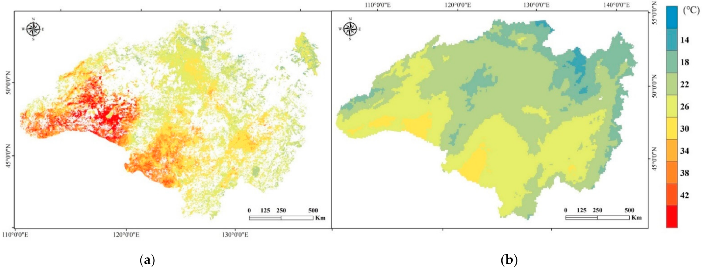
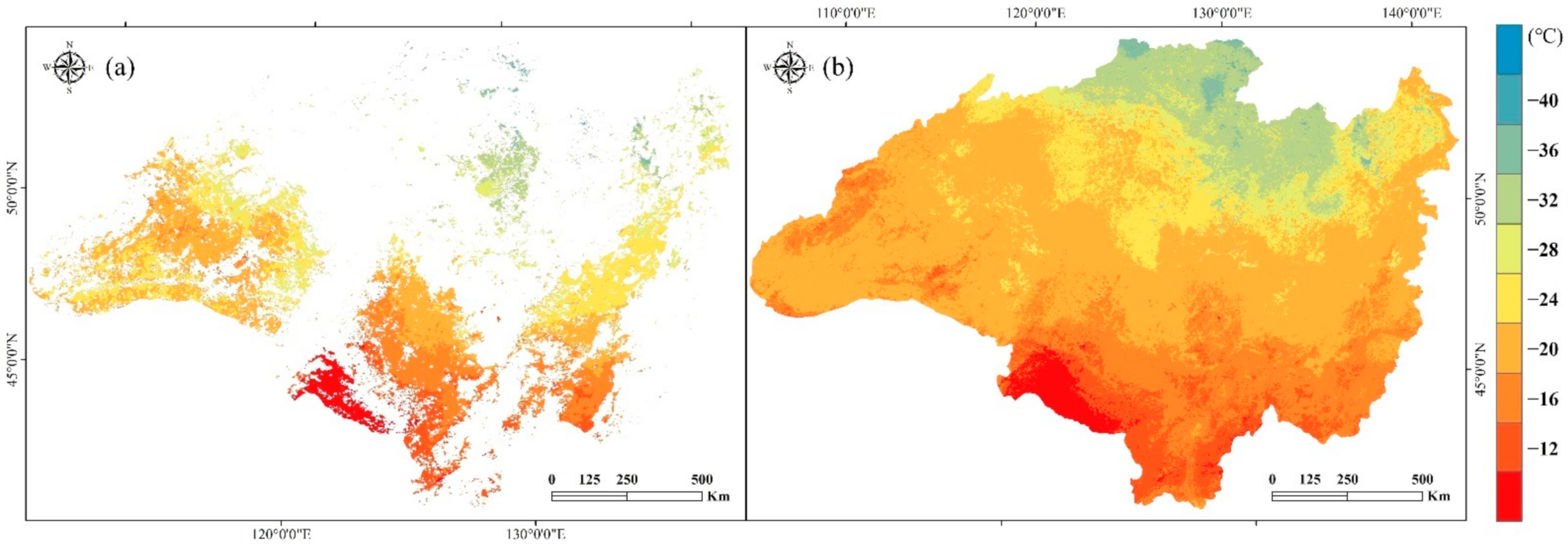
Figure 2 demonstrates the similarities and differences between the MODIS LST (a) and ERA5ST (b) on the same Day of Year (DOY) 193, 2010 in the peak summer of the study area. Overall, the ERA5ST was lower than MODIS LST. For example, one meteorological station (Tailai) is located in the warmer southwest of the study area. Its daily maximum temperature, minimum temperature, and average temperature were 45.5 °C, 18.0 °C, and 40.8 °C, respectively, on DOY 193, 2010. At this location, the MODIS LST was 34.2 °C and the ERA5ST was 26.1 °C (both at around 10:30 a.m. local time). This was reasonable because the reanalysis data were generally smoothed at much larger cells on land surface. Nevertheless, both datasets presented comparable geographical patterns with lower temperature in the north (above 50°N) and higher in the south. This agreement on global patterns makes it possible to fuse the two datasets for gap filling in this study. The missing local patterns in the ERA5ST data could be explained by satellite-extracted land surface information, as described later. Figure 2a also reveals a dramatic number of missing pixels in MODIS LST. Therefore, gap-filling is necessary before it can be used as a valid LST source in further studies.
This study explored the relationship between the MODIS LST and ERA5ST values at valid samples. A GAM approach was developed that focuses on quantifying the differences between the two products by exploring the environmental impacts in different seasons. It is expected to compensate for the underestimation of ERA5ST for improved gap filling. As a generalized predictive model, GAM allows for the additivity of non-linear functions of the covariates (i.e., the environmental parameters in this study). Given the additivity with covariate-specific smoothing functions, it could effectively reduce the estimation bias from multiple covariates in the regression [45].
The difference between ERA5ST and MODIS LST (further denoted as ΔLST) was defined as the dependent variable, ΔLST = MODIS LST−ERA5ST (unit in Celsius). Six environmental parameters (NDWI, NDVI, NDSI, longitude, latitude, and DEM) served as independent variables (covariates). NDWI explains the influence of surface wetness to land surface thermal process. NDVI has proven to be closely related to vegetation density and productivity, which presents the effect of vegetation conditions on the thermal processes. The Amur River Basin is located in a high-latitude cold region where snow cover characterizes its cold days. NDSI reflects the snow-covered condition. Elevation explains the LST variation in different terrains such as mountains and plains of the study area. Given the large geographic extent of the study area, longitude and latitude were also included in the model to pick up the LST variation at different locations.
The model was developed in two seasons to better reflect the seasonal land cover variations in a cold region: a growing season from April to September and snowing season from October to March [46]. NDVI was only applied in the growing season while NDSI was only used in the snowing season. Additionally, to test the influence of different land cover types on the thermal process, each of the three primary land covers (forest, grassland, and agriculture land) was examined in the models in the growing season. The equations are as follows:
Growing season:
Δ LST g , c = β 0 + s 1 NDWI c + s 2 NDVI c + s 3 DEM c + s 4 Lon c + s 5 Lat c +
Snowing season:
Δ LST s = β 0 + s 1 NDWI + s 2 NDSI + s 3 DEM + s 4 Lon + s 5 Lat +
where c represents the three land cover types, c = forest, grassland, agricultural land, respectively. The term g represents growing season and s represents snowing season. s1, s2, s3, s4, s5 are covariate-dependent spline smoothing functions that optimize the fitting and control the smoothness. In growing season, NDVI < 0 means no vegetation cover. In the snowing season, NDSI < 0 means no snow cover. In both seasons, all pixels with NDVI or NDSI less than 0 were assigned to 0. The DEM, lon, and lat variables were normalized to the [0,1] range. The term represents the simulation noises in each model.
Once the GAM models are established, the missing MODIS LST pixels in each season can be filled by compensating the simulated ΔLST to ERA5ST at each pixel. The equations are as follows:
LST g , c =   Δ LST g , c + ERA 5 ST
LST s =   Δ LST s + ERA 5 ST
where LSTg,c and LSTs are the gap-filled LST pixels in the growing season and snowing season, respectively. The ΔLSTg,c and ΔLSTs are the GAM-simulated difference between MODIS LST and ERA5ST.
The gap-filled MODIS LST data series in 2010 were compared with the valid pixel samples. Recall that 30% of the valid pixel samples were used as validation points of this study. At these points, both the original MODIS LST and the gap-filled LST were extracted. The scatterplots in both growing season (three land cover types) and snowing season (all land covers) were extracted to visually compare the agreement. A commonly applied statistical indicator, the root mean square error (RMSE), was calculated:
RMSE = i = 1 n T o r i T g f i 2 n
where n is the total number of validation samples. Tor(i) and Tgf(i) represent original MODIS LST and the gap-filled LST value of sample i, respectively.

3. Results and Discussion

3.1. Characteristics of the LST Data in the Study Area

Statistical analyses of all valid pixel samples were carried out (Table 2). Agreeing with the visual comparison in Figure 2 above, the MODIS LST was significantly higher than ERA5ST. In the growing season, the difference varied with land covers, with 8.0 °C in forests, 11.0 °C in agriculture lands, and 13.0 °C in grasslands in growing season; the standard deviations of both products were similar in all land covers. In the snowing season, although the difference of mean LST (4.8 °C) was lower than that of growing season, the standard deviations of both products were much higher, with 13.6 °C in MODIS LST and 10.0 °C in ERA5ST, indicating a higher degree of dispersion of LST in the snowing-season. It is reasonable to assume that this large dispersion may come from local environmental heterogeneity across the study area.
Data missing in the MODIS LST products is a commonly observed problem. For gap-filling purposes, this study defined all LST pixels with noise flags in a MODIS LST image as missing data. At the 8-day interval, the percentage of missing data at a given pixel was calculated as the ratio of the occurrence of missing data over the examined time period (growing season, snowing season, or the whole year). Statistically, missing data in the growing season accounted for 31.3% and that in the snowing season accounted for 57.5% of the entire valid sample set. Of the samples in the growing season, missing data accounted for 55.2%, 35.2%, and 30.5% in forest, grassland, and agricultural land, respectively.
Geographically, missing data in the growing season (Figure 3a) were much less than in the snowing season (Figure 3b). In the growing season of the study area, most of the precipitation is in summer in a monsoon climate and therefore, cloud cover is the primary source of missing data. In the snowing season (Figure 3b), the higher percentage of missing data is mainly located in the mountain forests where snow-induced noises may play a significant role. In some areas, the LST data were almost missed across the snowing season (100%). The year-long percent map (Figure 3c) revealed that the cold region suffered from a large extent of frequent data missing, especially in the snow season, which needs to be gap-filled to improve the quality of MODIS LST products.
The impacts of cloud and snow were further explored. The number of cloud days in 2010 was extracted from the Cloud State flag in MOD09GA. The cloud days in the growing season had a range of 60–120 days out of the six months (Figure 4a), while those in the snowing season could reach 150 days (Figure 4b). The longer cloud days in the snowing season may be attributed to the influence of snow-induced noises, especially in forest lands. Over the whole year of 2010 (Figure 4c), the majority of areas in the basin were covered with cloud for more than six months (180–240 days). Mountainous areas tended to have more cloud days, for example, the Yablonovyy Mountains in the west end, the Greater Khingan Mountains in the middle, Changbai Mountains in the southwest, and Bureinsky Ridge at the east of the basin. At higher altitudes of mountains ranges, the warm and humid air currents from the Pacific monsoon are uplifted by the topography, resulting in more cloud days than other areas at lower elevation. Figure 4 confirms the necessity of gap filling to correct the cloud noises of the MODIS LST product in this region.
Winter snow is a unique characteristic of the high-latitude cold region and deserves further analysis. Referring to past studies, snow pixels were extracted with NDSI > 0.4 [47,48]. In the one-year period of 2010, the snow-covered days at a given pixel were calculated as the count of the snow occurrence in the 46 MODIS scenes multiplied by 8. The number of snow-covered days in the growing season were reasonably low in the warm months of April–September (Figure 5a). In the snowing season, most of the basin had snow covering more than 96 days (Figure 5b). Areas with the most snow-cover days were concentrated in the north of the basin at higher latitudes (the red areas in Figure 5b). The snow-cover days in Figure 5b had a similar pattern to the cloud cover days in Figure 4b, confirming that snow can be attributed to missing pixels of the MODIS LST.

3.2. GAM Simulation: Relationships between ΔLST and Covariates

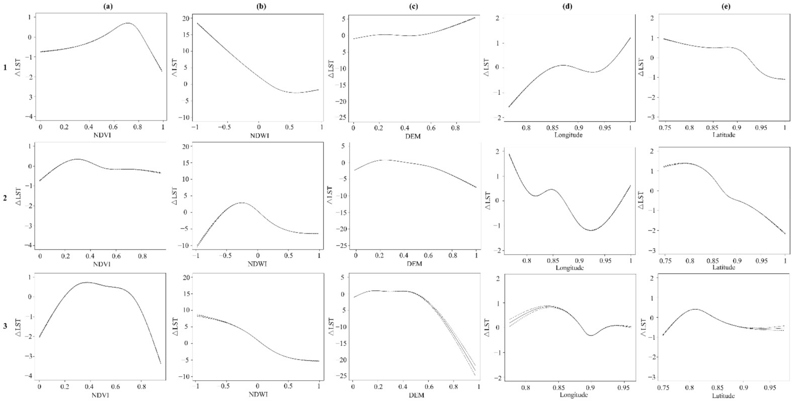
One attractive feature of GAM is that it can decompose and inspect the contribution of each covariate via a partial dependence function to the overall prediction. Figure 6 shows how ΔLST varies with each covariate in the model simulation in the growing season. The solid line is ΔLST explained by the covariate. The dotted lines represent the 95% confidence envelopes. All relationships in Figure 6 are statistically significant (p < 0.001).
For NDVI (Figure 6(a1–a3)), its relationship with ΔLST is bi-directional in all three land cover types (forest, grassland, agriculture), with a positive one in lower NDVI and negative one in higher NDVI. This is reasonable since land surface temperature increases rapidly early in the growing season. When vegetation reaches its peak growth (high NDVI), the cooling impact of vegetation becomes apparent, especially in forests and agricultural fields that have denser covers than grasslands. This impact was better picked up by including NDVI in the GAM model. However, the contribution of NDVI to ΔLST was mostly limited (in a range of [−1–1] °C), except in agriculture lands. This may be attributed to the limited spatial heterogeneity of NDVI within forests and grasslands. Agriculture lands in this region are irrigated in the growing season, which can explain up to −3 °C of ΔLST with higher NDVI.
For NDWI (Figure 6(b1–b3)), it had a strong negative relationship in forest and agricultural lands, revealing that land surface wetness plays a significant role in reducing LST. Among the three land covers, land surface wetness in forest lands (primarily in form of leaf moisture) was the most important factor that explained a ΔLST range of [−5–15] °C. Land surface moisture in agriculture lands could be soil moisture (including irrigation) and crop leaf moisture, which also explains a good range of ΔLST. Grasslands usually have a lower biomass under less human management than agricultural fields. Its positive relationship in lower NDWI (drier condition) may be similar to that of NDVI in the early growing season, which is highly affected by rapid LST increase. Meaningfully, when NDWI > 0.0, land surface wetness effectively explains ΔLST in a similarly negative relationship such as forests and agricultural lands, although the relationship is in a lower amplitude (in a ΔLST range of [−5–3] °C).
For DEM (Figure 6(c1–c3)), its relationship with ΔLST is highly land cover dependent. This local topographic feature was not picked up in the ERA5ST simulation. Therefore, DEM plays an important role in explaining ΔLST between the two products. Forests in the study area are typical northern forests growing on mountainous terrain. It positively attributes to the ΔLST variation, especially in areas with higher elevation (Figure 6(c1)). Grasslands are dominated in Mongolia Plateau. Grasses in lower elevation usually has better growth that is associated with the lower surface temperature. In this sense, DEM in grasslands explains the negative relationship with ΔLST (Figure 6(c2)). Agriculture cultivation is mostly in flat plains where DEM variation is limited, so does not play a significant role except in some agriculture fields at higher elevations (Figure 6(c3)). In these less representative agriculture lands, higher uncertainties (large ± 95% confidence envelops) can be observed on the strongly negative relationship.
Longitude (Figure 6(d1–d3)) and latitude (Figure 6(e1–e3)) explain limited ΔLST variation (mostly within [−1–1] °C), although some local relationships were observed in each land cover type. We decide to keep these two covariates in model simulation to pick up these local variations.
Overall, in the growing season, land surface wetness (NDWI) plays the strongest role, followed by DEM and NDVI, in explaining the LST differences between MODIS LST and ERA5ST. The covariate-specific relationships in GAM models vary with land covers. The cooling effect of land surface wetness is nicely reflected in a strong, negative relationship between ΔLST and NDWI, due primarily to thermal reduction from land surface wetness including leaf water content and soil moisture, especially in forests and agriculture lands. Vegetation (NDVI) is less useful in forests and grasslands where human interference is limited. DEM has a recognizable impact on forests and grasslands, but not less than on agriculture lands, which are mostly in plain areas. Although longitude and latitude have limited power in explaining the ΔLST, they possess some local relationships in each land cover type.
In the snowing season, NDSI replaced NDVI and the three land cover types were not separately modeled in GAM analysis. In the partial dependent plots (Figure 7), all relationships were statistically significant (p < 0.001). NDSI had an omni-directional negative relationship with ΔLST (Figure 7a), indicating that it fairly recognized the decreased LST along with increased snow cover, a unique feature in high-latitude cold land, but has not been analyzed in the ERA5ST product. Including NDSI in the GAM model effectively corrects the snow-induced LST variations. The impact of NDWI on ΔLST (Figure 7b) was similar to that of grasslands in the growing season, having a positive relationship with ΔLST in drier lands and negative when surface wetness increased. The right tail in Figure 7b resembles the one in Figure 7a, which is reasonable because snow cover and land surface wetness are corelated in nature. Since all land cover types are considered in one simulation, Figure 7c reflects a bi-directional relationship between DEM and ΔLST. Similar to the growing season, longitude (Figure 7d) and latitude (Figure 7e) did not explain much of the ΔLST. Overall, GAMs in the snowing season described less ΔLST variation (in a range of [−3–3] °C), but NDSI revealed a distinctly negative relationship and was an important covariate in the model. NDWI and DEM also explained a fair amount of localized LST variations between the two products.
Table 3 summarizes the statistical summaries of GAM simulated ΔLST using the training samples. The R2 values ranged from 0.46 to 0.56 in both seasons. Given the extremely large sample sizes, the R2 values of all models were relatively low. However, all models were statistically significant (p < 0.001). In the growing season, the RMSE ranged from 2.5 °C to 3.0 °C in the three land cover types. Forest lands reached the lowest RSME, followed by grasslands and agricultural lands. Model performance in the growing season was slightly better than the snowing season, which had a RMSE of 3.4 °C. A higher amount of missing data were observed in the snowing season, which may be attributed to its higher RMSE of the model.
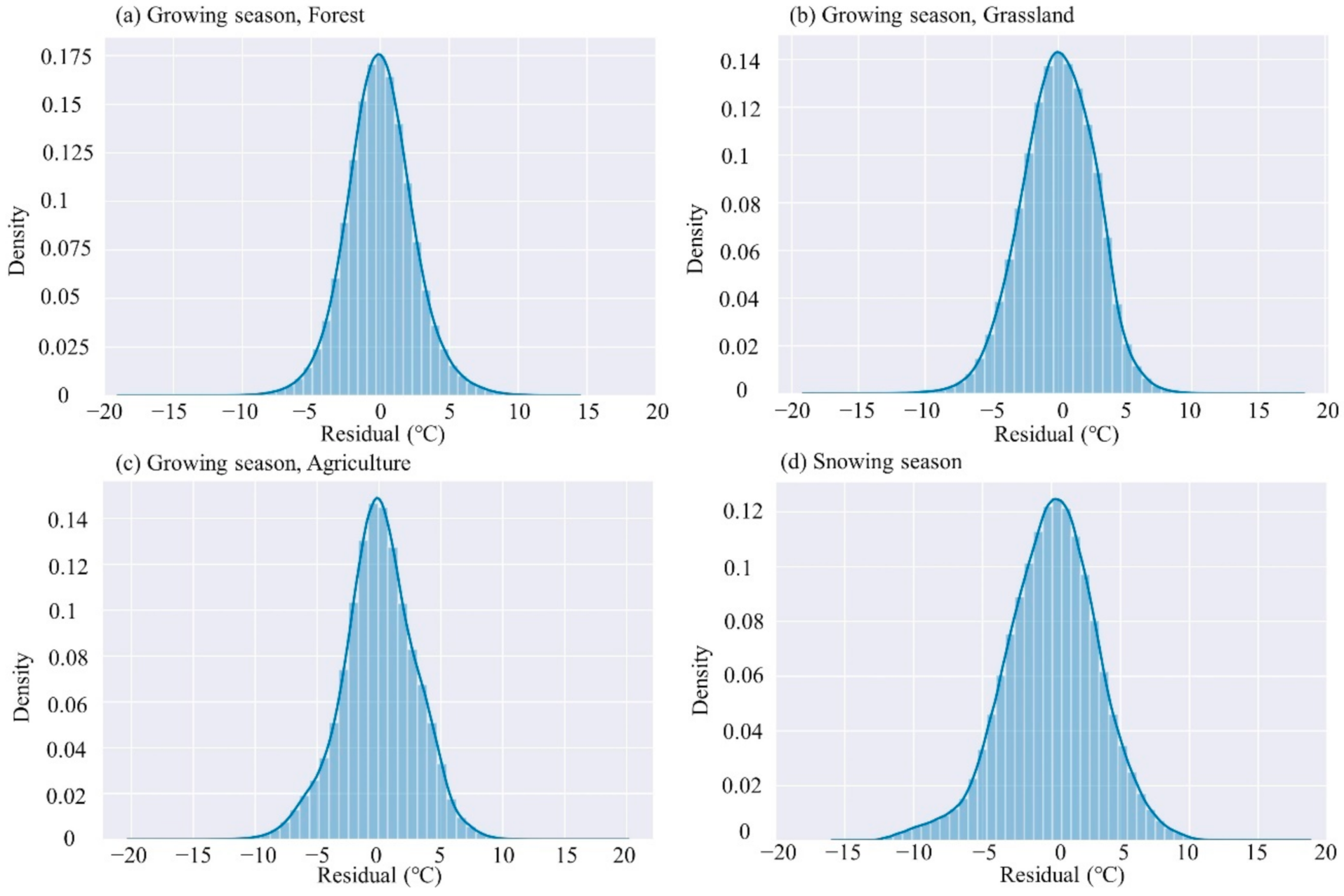
The mean observed and mean simulated ΔLST values are basically the same in Table 3. This was confirmed in the residual plots (Figure 8). The residuals of all GAM models (observed ΔLST − simulated ΔLST) were symmetrically distributed (Figure 8), indicating the randomness of simulation errors. While centered at ΔLST = 0 °C, all plots revealed reasonable deviations. In the growing season, the residues of three land cover types had similar dispersion (95% significance interval) with ±4.9 °C in forests, ±5.4 °C in grasslands, and ±5.8 °C in agricultural lands, respectively. With all land covers considered in one model, residues in the snowing season had a slightly wider dispersion of ±6.6 °C. In all models, tails of large residues in both directions may be related to the mismatching between MODIS LST pixels and the resampled ERA5ST pixels, especially in areas with mixed land covers.

3.3. Gap-Filled MODIS LST Products

The missing pixels in each MODIS LST image were filled by adding the GAM simulated ΔLST to the resampled ERSA5ST values. The valid MODIS LST pixels remained unchanged. We randomly selected one image in the growing season and one in the snowing season to visually demonstrate the gap-filling performance. In the peak growing season on 4 July 2010 (Figure 9), the ERA5ST image (Figure 9a) had a continuous distribution at coarse spatial resolution. In agreement with Table 2 above, it had a significantly lower temperature than MODIS LST. In the MODIS LST image (Figure 9b), missing pixels counted into 63% of the basin. After gap-filling, the resulting image (Figure 9c) maintained good spatial consistency across the entire basin.
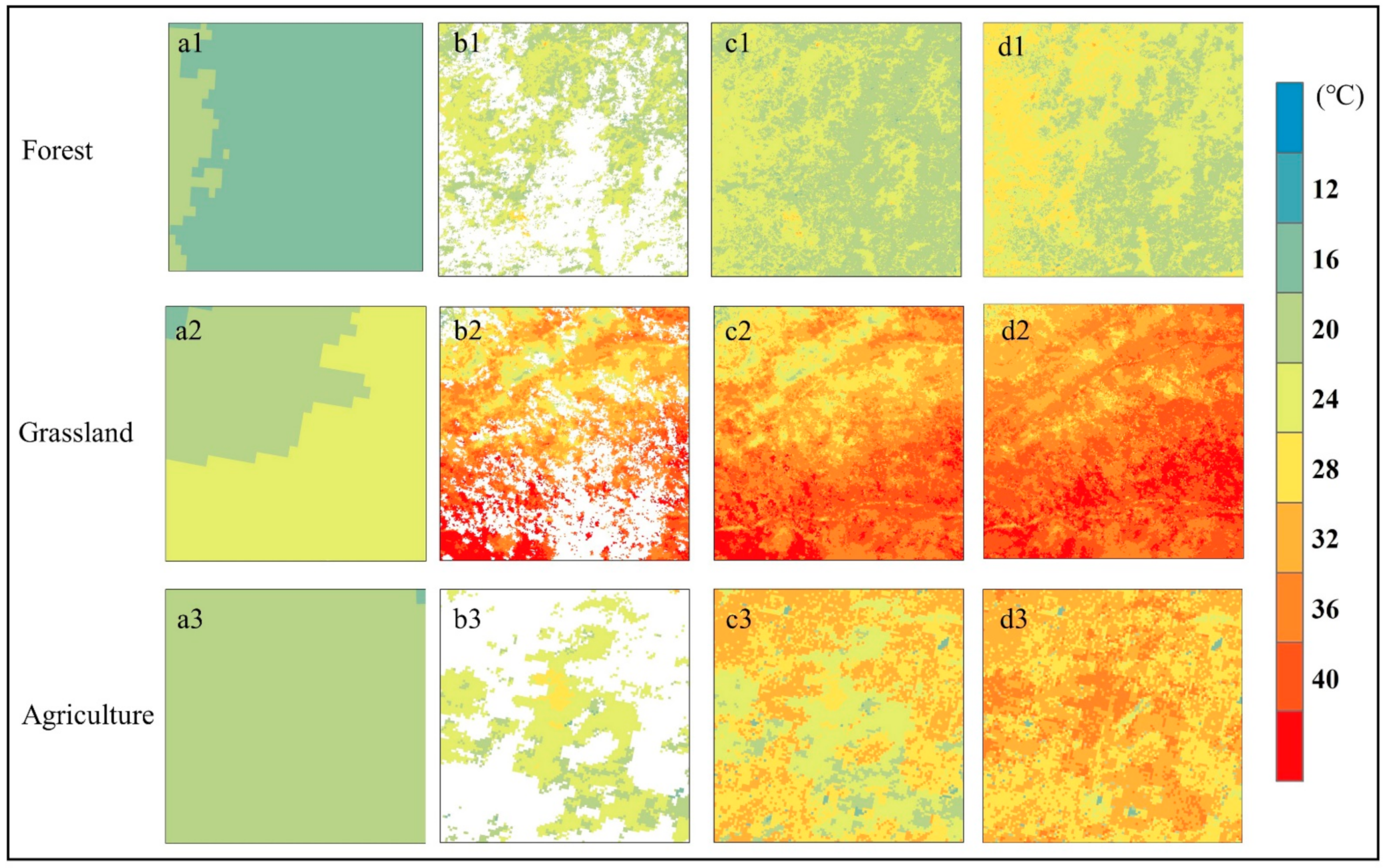
Three subsets were randomly selected in Figure 9 for detailed visual comparison, one for each land cover type (Figure 10). Each subset had a relatively homogeneous distribution in the ERA5ST data, but more details were observed in the MODIS LST. Subset 1 represents a typical northern forest in the Eurasia region. It has an average temperature of 18.3 °C in ERA5ST (Figure 10(a1)) and 24.1 °C in the original MODIS LST excluding the missing pixels (Figure 10(b1)). After gap filling, it had an average temperature of 23.8 °C (Figure 10(c1)). Both the ERA5ST and gap-filled MODIS LST reflected an increasing trend of LST from the east to west of the subset, but the MODIS LST revealed apparently more details than ERA5ST. Subset 2 is a typical grassland on the Mongolian Plateau. Its average temperature was 24.5 °C in ERA5ST (Figure 10(a2)), 35.8 °C in the original MODIS LST (Figure 10(b2)), and 36.4 °C after gap-filling (Figure 10(c2)). Similarly, the GAM model picks up the local increasing trends from north to south in the gap-filled product. In the agriculture subset (subset 3), its average temperature was 20.7 °C in ERA5ST (Figure 10(a3)), 25.2 °C in original MODIS LST (Figure 10(b3)), and 29.3 °C after gap-filling (Figure 10(c3)). While the subset had a homogeneous ERA5ST distribution, the localized variations were also successfully picked up in the gap-filled MODIS LST product. A visual comparison was also carried out for the fully simulated LST in the three subsets (Figure 10(d1–d3)). As expected, the simulated LST maintained a similar pattern to the gap-filled output (Figure 10(c1–c3)), but lacked the same level of detail in the valid pixels. Therefore, this study kept the original LST values in the valid pixels, and only filled the gaps of missing pixels.
In the peak snowing season on 25 January 2010 (DOY 25), the MODIS LST missing data accounted for 72.0% in the basin (Figure 11a). Similarly, the LST was continuously distributed after gap-filling (Figure 11b). Due to an extreme number of missing pixels, the gap-filled distribution on DOY 25 showed less local details than that on DOY 185 (as shown in Figure 9c). Nevertheless, it revealed the clear decreasing trend in temperature from the north to south in such a large basin. Several hot and cold spots of LST in this specific day could also be observed. Figure 9 and Figure 11 reveal that GAM simulation effectively removed missing pixels and produced continuous LST data in the study area.

3.4. Error Assessment

The GAM-filled LST product was visually compared with the results from regular linear interpolation that was commonly used in gap-filling methods. Here, we adopted the inverse distance weighted (IDW) technique in the spatial analysis module of ArcGIS. For the same MODIS LST image on DOY 185 used in Figure 9 and Figure 10, twelve nearest valid LST pixels were used to perform interpolation at any gap pixel. The valid LST pixels at a longer distance from the gap pixel contributed less to the calculation.
In Figure 12b, the IDW approach filled all gaps in the original MODIS LST image (Figure 12a) and effectively revealed the major clusters across the study region. When compared with the GAM-filled product (as shown in Figure 9c), its LST distributions turned to be polygonized affected by the weighted distance to nearby valid pixels. This phenomenon was more obvious in areas with large gaps such as the east part of the study region. Rather, the LST patterns in the GAM-filled product (Figure 9c) had a smoother background while the hot spots remained. The polygonized effects in the IDW-filled LST were visually distinct in the three subsets of forest (1), grassland (2), and agriculture land (3). More specifically, the agriculture subset had a large proportion of gaps. In this case, the IDW filling became insufficient in extracting the LST details due to the lack of neighboring information. Rather, the GAM-filled results effectively preserved these localized LST variations. Therefore, the proposed GAM approach performed better than regular linear interpolation.
With the validation samples (30% of valid pixel samples), the original MODIS LST and GAM simulated LST were compared (Figure 13). In the scatterplots, color density indicates the concentration of sample points. Most sample points were close to the 1:1 line, indicating good agreement between the original MODIS LST and simulated LST. The RMSE in the growing season was less than 3 °C. Among the three land cover types, forest (Figure 13a) had the lowest RMSE of 2.5 °C. Grassland (Figure 13b) and agricultural land (Figure 13c) were spatially more heterogeneous and were subject to various cropping management, which may be attributed to the slightly higher RMSEs than forest land. The average RMSE in the growing season was 2.7 °C. In Figure 13d, the simulated LST in the snowing season had a higher RMSE (3.4 °C) than those in the growing season, which agreed with the statistical results in model development. Additionally, its scatterplot revealed two high-density hot spots when land cover types were not separately considered in the snowing season.
Finally, while this study utilized the ERA5ST product as a reference for gap filling, the re-analyzed skin temperature was different from the satellite-retrieved MODIS land surface temperature. Figure 14 compares the resampled ERA5ST and MODIS LST using the validation samples. Although all scatterplots revealed significant linear relationships, the ERA5ST values were universally lower than MODIS LST in both seasons. The difference varied with land cover types in growing season, in which forest (Figure 14a) had the least RSME of 8.7 °C. Similar to Figure 13, higher RMSE values were observed in grassland (14.1 °C, Figure 14b) and agriculture land (12.1 °C, Figure 14c), which were less spatially uniform than forest land. Consideration of land cover types is necessary in the gap filling of MODIS LST data to compensate for the spatial heterogeneity in the growing season. Greenness in the snowing season is limited and therefore, land covers play a less significant role. The difference between the two products had the lowest RMSE of 6.9 °C, even when all land covers were considered in the comparison (Figure 14d).
With the strong linear relationships in Figure 14, this study confirms that ERA5ST could serve as a valid reference for gap filling of the MODIS LST product. The feasibility of ERA5ST in gap filling has been explored in recent studies such as Dumitrescu et al. [29] which embraced the elevation, time, and solar radiation into the GAM model. Beyond that, our study took advantage of high-resolution satellite imagery to blend land surface information like wetness and greenness into the model. This information varied with land cover types and physiological characteristics and therefore, highlighted the local patterns that could not be observed in coarse-resolution reanalysis data. More specifically, this study demonstrated that snow cover in the high-latitude region could be a unique addition to the gap-filling model, which has not been well investigated in previous studies. Given the hourly, global availability of the ERA products and daily high-resolution optical imagery in various missions, the GAM simulation approach explored in this study could be adapted to fill the gaps of other satellite-extracted, cloud-contaminated LST products for regional and global studies.

4. Conclusions

MODIS LST products have been recognized as a reliable source of high-resolution (km scale) land surface temperature in various studies. The missing pixels in these thermal products, however, hinder their widespread utilization. This study explored a gap-filling approach to correcting the missing MODIS LST pixels from the 0.1° grid ERA5ST product in a high-latitude cold region. Three environmental indices (NDVI, NDWI, NDSI) were extracted to approximate the impacts of vegetation, land surface wetness, and snow cover that have not been well examined in the ERA5ST datasets. Terrain and locational variations in this large geographic region were also considered. A generalized additive model (GAM) was established to simulate the contributions of these covariates to the difference between MODIS LST and ERA5ST (ΔLST) in the growing season (vegetation was added) and the snowing season (snow was added), respectively. Primary findings include:
(1)
The MODIS LST and ERA5ST hold similar image-wide patterns of land surface temperature. Still, there were locally varying differences between the two products, with MODIS LST 8.0–13.0 °C higher in the growing season and 4.8 °C higher in the snowing season. These ΔLST differences could be explained by satellite-extracted land surface information.
(2)
Land surface wetness (i.e., NDWI) had the highest importance in explaining the ΔLST between the two products. The MODIS LST was significantly lower than ERA5ST on the moist surface (high NDWI) of all land cover types, indicting the cooling effect of land surface wetness that is not picked up in the ERA5ST dataset.
(3)
In winter months, snow (NDSI) impact on LST cannot be ignored in this typical high-latitude cold land. With a negatively linear relationship in its partial dependent function, the GAM model effectively explains the lower MODIS LST than ERA5ST when snow presents.
(4)
Other environmental variables also contribute to the model. Elevation is important in both seasons, but its partial dependent functions are land cover dependent. Vegetation possesses weak but stable relationships with ΔLST in all land cover types. Longitude and latitude obtained some localized ΔLST variations.
With these seasonal and environmental characteristics considered, the GAM approach in this study effectively corrects the differences between MODIS LST and ERA5ST with the R2 in a range of 0.46–0.56 in the model simulation. With the validation samples, the RMSE reached an average of 2.7 °C in the growing season and 3.4 °C in the snowing season. The models performed better in forests than grasslands and agriculture lands, and better in the growing season than the snowing season. The gap-filled MODIS LST products provide crucial information for studying surface thermal processes in high latitude cold regions.

Author Contributions

Conceptualization, C.W., and D.G.; Programming, D.G.; Validation, D.G., Z.L., and Y.L.; Data analysis, D.G., C.W., and S.Z.; Data curation, D.G.; Writing—original draft preparation, D.G.; Writing—review and editing, C.W., S.Z., and J.H.; Project administration, S.Z.; Funding acquisition, S.Z. All authors have read and agreed to the published version of the manuscript.

Funding

This research was funded by the Key Joint Program of the National Natural Science Foundation of China (NSFC) and Heilongjiang Province for Regional Development [No. U20A2082]; National Natural Science Foundation of China (NSFC) [No. 4197115]; and the Natural Science Foundation of Heilongjiang Province of China [No. TD2019D002].

Conflicts of Interest

The authors declare no conflict of interest.

References

  1. Anderson, M.; Norman, J.; Kustas, W.; Houborg, R.; Starks, P.; Agam, N. A thermal-based remote sensing technique for routine mapping of land-surface carbon, water and energy fluxes from field to regional scales. Remote Sens. Environ. 2008, 112, 4227–4241. [Google Scholar] [CrossRef]
  2. Kustas, W.; Anderson, M. Advances in thermal infrared remote sensing for land surface modeling. Agric. For. Meteorol. 2009, 149, 2071–2081. [Google Scholar] [CrossRef]
  3. Li, Z.-L.; Tang, B.-H.; Wu, H.; Ren, H.; Yan, G.; Wan, Z.; Trigo, I.F.; Sobrino, J.A. Satellite-derived land surface temperature: Current status and perspectives. Remote Sens. Environ. 2013, 131, 14–37. [Google Scholar] [CrossRef] [Green Version]
  4. Langer, M.; Westermann, S.; Boike, J. Spatial and temporal variations of summer surface temperatures of wet polygonal tundra in Siberia-implications for MODIS LST based permafrost monitoring. Remote Sens. Environ. 2010, 114, 2059–2069. [Google Scholar] [CrossRef]
  5. ERA5-Land Data Documentation. Available online: https://confluence.ecmwf.int/display/CKB/ERA5-Land%3A+data+documentation (accessed on 20 March 2021).
  6. Johannsen, F.; Ermida, S.; Martins, J.; Trigo, I.F.; Nogueira, M.; Dutra, E. Cold Bias of ERA5 Summertime Daily Maximum Land Surface Temperature over Iberian Peninsula. Remote Sens. 2019, 11, 2570. [Google Scholar] [CrossRef] [Green Version]
  7. Wang, X.; Chen, D.; Pang, G.; Ou, T.; Yang, M.; Wang, M. A climatology of surface–air temperature difference over the Tibetan Plateau: Results from multi-source reanalyses. Int. J. Climatol. 2020, 40, 6080–6094. [Google Scholar] [CrossRef] [Green Version]
  8. Wan, Z. New refinements and validation of the MODIS Land-Surface Temperature/Emissivity products. Remote Sens. Environ. 2008, 112, 59–74. [Google Scholar] [CrossRef]
  9. Wan, Z.; Zhang, Y.; Zhang, Q.; Li, Z.L. Quality assessment and validation of the MODIS global land surface temperature. Int. J. Remote Sens. 2010, 25, 261–274. [Google Scholar] [CrossRef]
  10. Hu, L.; Brunsell, N.A.; Monaghan, A.J.; Barlage, M.; Wilhelmi, O.V. How can we use MODIS land surface temperature to validate long-term urban model simulations? J. Geophys. Res. Atmos. 2014, 119, 3185–3201. [Google Scholar] [CrossRef] [Green Version]
  11. Jin, M. Interpolation of surface radiative temperature measured from polar orbiting satellites to a diurnal cycle: 2. Cloudy-pixel treatment. J. Geophys. Res. Atmos. 2000, 105, 4061–4076. [Google Scholar] [CrossRef]
  12. Shen, H.; Li, X.; Cheng, Q.; Zeng, C.; Yang, G.; Li, H.; Zhang, L. Missing Information Reconstruction of Remote Sensing Data: A Technical Review. IEEE Geosci. Remote Sens. Mag. 2015, 3, 61–85. [Google Scholar] [CrossRef]
  13. Mukherjee, S.; Joshi, P.K.; Garg, R.D. Regression-Kriging Technique to Downscale Satellite-Derived Land Surface Temperature in Heterogeneous Agricultural Landscape. IEEE J. Sel. Top. Appl. Earth Obs. Remote Sens. 2015, 8, 1245–1250. [Google Scholar] [CrossRef]
  14. Ozelkan, E.; Bagis, S.; Ozelkan, E.C.; Ustundag, B.B.; Yucel, M.; Ormeci, C. Spatial interpolation of climatic variables using land surface temperature and modified inverse distance weighting. Int. J. Remote Sens. 2015, 36, 1000–1025. [Google Scholar] [CrossRef]
  15. Yang, J.; Wang, Y.; August, P. Estimation of Land Surface Temperature Using Spatial Interpolation and Satellite-Derived Surface Emissivity. J. Environ. Inform. 2004, 4, 40–47. [Google Scholar] [CrossRef]
  16. Neteler, M. Estimating Daily Land Surface Temperatures in Mountainous Environments by Reconstructed MODIS LST Data. Remote Sens. 2010, 2, 333–351. [Google Scholar] [CrossRef] [Green Version]
  17. Ke, L.; Ding, X.; Song, C. Reconstruction of Time-Series MODIS LST in Central Qinghai-Tibet Plateau Using Geostatistical Approach. IEEE Geosci. Remote Sens. Lett. 2013, 10, 1602–1606. [Google Scholar] [CrossRef]
  18. Duan, S.-B.; Li, Z.-L.; Tang, B.; Wu, H.; Tang, R. Generation of a time-consistent land surface temperature product from MODIS data. Remote Sens. Environ. 2014, 140, 339–349. [Google Scholar] [CrossRef]
  19. Fan, X.-M.; Liu, H.-G.; Liu, G.-H.; Li, S.-B. Reconstruction of MODIS land-surface temperature in a flat terrain and fragmented landscape. Int. J. Remote Sens. 2014, 35, 7857–7877. [Google Scholar] [CrossRef]
  20. Zeng, C.; Long, D.; Shen, H.; Wu, P.; Cui, Y.; Hong, Y. A two-step framework for reconstructing remotely sensed land surface temperatures contaminated by cloud. ISPRS J. Photogramm. Remote Sens. 2018, 141, 30–45. [Google Scholar] [CrossRef]
  21. Cui, Y.; Ma, S.; Yao, Z.; Chen, X.; Luo, Z.; Fan, W.; Hong, Y. Developing a Gap-Filling Algorithm Using DNN for the Ts-VI Triangle Model to Obtain Temporally Continuous Daily Actual Evapotranspiration in an Arid Area of China. Remote Sens. 2020, 12, 1121. [Google Scholar] [CrossRef] [Green Version]
  22. Xu, Y.; Shen, Y. Reconstruction of the land surface temperature time series using harmonic analysis. Comput. Geosci. 2013, 61, 126–132. [Google Scholar] [CrossRef]
  23. Zhou, J.; Jia, L.; Menenti, M. Reconstruction of global MODIS NDVI time series: Performance of Harmonic ANalysis of Time Series (HANTS). Remote Sens. Environ. 2015, 163, 217–228. [Google Scholar] [CrossRef]
  24. Weiss, D.J.; Atkinson, P.M.; Bhatt, S.; Mappin, B.; Hay, S.I.; Gething, P.W. An effective approach for gap-filling continental scale remotely sensed time-series. ISPRS J. Photogramm. Remote Sens. 2014, 98, 106–118. [Google Scholar] [CrossRef] [PubMed] [Green Version]
  25. Kalyuzhnaya, A.; Nikitin, N.; Vychuzhanin, P.; Hvatov, A.; Boukhanovsky, A. Automatic evolutionary learning of composite models with knowledge enrichment. In Proceedings of the 2020 Genetic and Evolutionary Computation Conference Companion, Cancún, Mexico, 8–12 July 2020; pp. 43–44. [Google Scholar]
  26. Kang, M.; Ichii, K.; Kim, J.; Indrawati, Y.M.; Park, J.; Moon, M.; Lim, J.-H.; Chun, J.-H. New Gap-Filling Strategies for Long-Period Flux Data Gaps Using a Data-Driven Approach. Atmosphere 2019, 10, 568. [Google Scholar] [CrossRef] [Green Version]
  27. Buo, I.; Sagris, V.; Jaagus, J. Gap-Filling Satellite Land Surface Temperature Over Heatwave Periods With Machine Learning. IEEE Geosci. Remote Sens. Lett. 2021, 5. [Google Scholar] [CrossRef]
  28. Sarafanov, M.; Kazakov, E.; Nikitin, N.O.; Kalyuzhnaya, A.V. A Machine Learning Approach for Remote Sensing Data Gap-Filling with Open-Source Implementation: An Example Regarding Land Surface Temperature, Surface Albedo and NDVI. Remote Sens. 2020, 12, 3865. [Google Scholar] [CrossRef]
  29. Dumitrescu, A.; Brabec, M.; Cheval, S. Statistical Gap-Filling of SEVIRI Land Surface Temperature. Remote Sens. 2020, 12, 1423. [Google Scholar] [CrossRef]
  30. Ruiz-Álvarez, M.; Alonso-Sarria, F.; Gomariz-Castillo, F. Interpolation of Instantaneous Air Temperature Using Geographical and MODIS Derived Variables with Machine Learning Techniques. ISPRS Int. J. Geo-Inf. 2019, 8, 382. [Google Scholar] [CrossRef] [Green Version]
  31. Wood, S.N. Generalized Additive Models: An Introduction with R, 2nd ed.; Chapman and Hall/CRC: Boca Raton, FL, USA, 2017. [Google Scholar] [CrossRef]
  32. Aalto, J.; Pirinen, P.; Heikkinen, J.; Venäläinen, A. Spatial interpolation of monthly climate data for Finland: Comparing the performance of kriging and generalized additive models. Theor. Appl. Climatol. 2012, 112, 99–111. [Google Scholar] [CrossRef]
  33. Avis, C.A.; Weaver, A.J.; Meissner, K.J. Reduction in areal extent of high-latitude wetlands in response to permafrost thaw. Nat. Geosci. 2011, 4, 444–448. [Google Scholar] [CrossRef]
  34. Jin, H.; Yu, Q.; Lü, L.; Guo, D.; He, R.; Yu, S.; Sun, G.; Li, Y. Degradation of permafrost in the Xing’anling Mountains, northeastern China. Permafr. Periglac. Process. 2007, 18, 245–258. [Google Scholar] [CrossRef]
  35. MCD12Q1 MODIS/Terra+Aqua Land Cover Type Yearly L3 Global 500m SIN Grid V006. Available online: https://go.nasa.gov/3C3QrXc (accessed on 1 July 2021).
  36. Wan, Z.; Zhang, Y.; Zhang, Q.; Li, Z.-l. Validation of the land-surface temperature products retrieved from Terra Moderate Resolution Imaging Spectroradiometer data. Remote Sens. Environ. 2002, 83, 163–180. [Google Scholar] [CrossRef]
  37. Wan, Z. Collection-6 MODIS Land Surface Temperature Products Users’ Guide. Available online: https://lpdaac.usgs.gov/documents/118/MOD11_User_Guide_V6.pdf (accessed on 24 March 2021).
  38. Zhang, M.; An, J.; Zhang, J.; Yu, D.; Wang, J.; Lv, X. Enhanced Delaunay Triangulation Sea Ice Tracking Algorithm with Combining Feature Tracking and Pattern Matching. Remote Sens. 2020, 12, 581. [Google Scholar] [CrossRef] [Green Version]
  39. Wan, W.; Li, H.; Xie, H.; Hong, Y.; Long, D.; Zhao, L.; Han, Z.; Cui, Y.; Liu, B.; Wang, C.; et al. A comprehensive data set of lake surface water temperature over the Tibetan Plateau derived from MODIS LST products 2001-2015. Sci. Data 2017, 4, 170095. [Google Scholar] [CrossRef]
  40. Tucker, C.J. Red and photographic infrared linear combinations for monitoring vegetation. Remote Sens. Environ. 1979, 8, 127–150. [Google Scholar] [CrossRef] [Green Version]
  41. Hall, D.K.; Riggs, G.A.; Salomonson, V.V. Development of methods for mapping global snow cover using moderate resolution imaging spectroradiometer data. Remote Sens. Environ. 1995, 54, 127–140. [Google Scholar] [CrossRef]
  42. Gao, B.-c. NDWI—A normalized difference water index for remote sensing of vegetation liquid water from space. Remote Sens. Environ. 1996, 58, 257–266. [Google Scholar] [CrossRef]
  43. Hersbach, H.; Dee, D. ERA5 Reanalysis is in Production. Available online: https://www.ecmwf.int/en/newsletter/147/news/era5-reanalysis-production (accessed on 20 March 2021).
  44. de Rosnay, P.; Balsamo, G.; Muñoz Sabater, J.; Dutra, E.; Albergel, C.; Rodríguez-Fernández, N.; Hersbach, H. High Resolution Land Reanalysis. Available online: https://climate.copernicus.eu/sites/default/files/repository/Events/ECMWF_land_reanalysis_20160518.pdf (accessed on 20 March 2021).
  45. Hastie, T.J.; Tibshirani, R.J. Generalized Additive Models, 1st ed.; Chapman and Hall/CRC: London, UK, 1990. [Google Scholar]
  46. Li, H.; Wang, C.; Zhang, L.; Li, X.; Zang, S. Satellite monitoring of boreal forest phenology and its climatic responses in Eurasia. Int. J. Remote Sens. 2017, 38, 5446–5463. [Google Scholar] [CrossRef]
  47. Dozier, J. Spectral signature of alpine snow cover from the landsat thematic mapper. Remote Sens. Environ. 1989, 28, 9–22. [Google Scholar] [CrossRef]
  48. Riggs, G.A.; Hall, D.K.; Salomonson, V.V. A snow index for the Landsat Thematic Mapper and Moderate Resolution Imaging Spectroradiometer. In Proceedings of the IGARSS 94-1994 IEEE International Geoscience and Remote Sensing Symposium, Pasadena, CA, USA, 8–12 August 1994; Volume 1944, pp. 1942–1944. [Google Scholar]
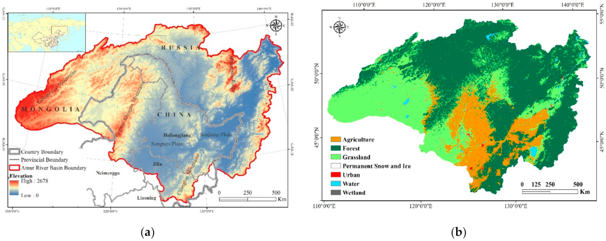
Figure 1. Geographical characteristics of the Amur River Basin (a) and its land cover distribution (b), modified from the MODIS MCD12Q1 product in 2010.
Remotesensing 13 03667 g001
Figure 2. Example maps of MODIS LST (a) and ERA5ST (b) on DOY193 (12 July), 2010 at 10:30 a.m. local time. The gaps in (a) are missing pixels.
Remotesensing 13 03667 g002
Figure 3. Percentage map of missing data in the MODIS LST image series in growing season (a), snowing season (b), and the whole year in 2010 (c).
Remotesensing 13 03667 g003
Figure 4. Spatial distribution of cloud cover days in the growing season (a), snowing season (b), and the whole year (c) in the basin.
Remotesensing 13 03667 g004
Figure 5. Snow-covered days in the growing season (a) and snowing season (b) in the basin. The white areas are water and other accessory land covers that are masked out.
Remotesensing 13 03667 g005
Figure 6. GAM analysis in the growing season: partial dependence plots of ΔLST for three land covers with five covariates: forest (1st row), grassland (2nd row), and agriculture land (3rd row). The columns represent the five covariates: NDVI (a), NDWI (b), DEM (c), longitude (d), and latitude (e).
Remotesensing 13 03667 g006
Figure 7. GAM analysis in snowing season: partial dependence plots of ΔLST with NDSI (a), NDWI (b), DEM (c), longitude (d), and latitude (e).
Remotesensing 13 03667 g007
Figure 8. Histograms of the residuals from GAM analysis for three land cover types in the growing season: forest (a), grassland (b), agriculture (c), and all training samples in the snowing season (d).
Remotesensing 13 03667 g008
Figure 9. Demonstration of gap filling on DOY 185 (4 July 2010): the ERA5ST (a), original MODIS LST (b), and gap-filled MODIS LST (c).
Remotesensing 13 03667 g009
Figure 10. Example subsets of ERA5ST (a1a3), original MODIS LST (b1b3), gap-filled MODIS LST (c1c3), and fully GAM-simulated LST (d1d3) on DOY 185 (4 July 2010).
Remotesensing 13 03667 g010
Figure 11. The LST image on DOY 25 before gap-filling (a) and after gap-filling (b).
Remotesensing 13 03667 g011
Figure 12. Comparison of the GAM-filled LST and the IDW-interpreted LST on DOY 185 (4 July 2010). The original MODIS LST is in (a) and the IDW-interpreted LST is in (b). The three subsets, forest (1), grassland (2), and agricultural land (3), reveal the visual differences between the two approaches.
Remotesensing 13 03667 g012
Figure 13. Scatterplots of the original MODIS LST and simulated LST for forest (a), grassland (b), and agriculture land (c) in the growing season and all land cover types in the snowing season (d). The black line represents the 1:1 line.
Remotesensing 13 03667 g013
Figure 14. Scatterplots of the MODIS LST and resampled ERA5ST with validation samples for forest (a), grassland (b), and agriculture land (c) in the growing season and all land cover types in the snowing season (d). The black line represents the 1:1 line.
Remotesensing 13 03667 g014
Table 1. Primary land cover classes over the study area.
Land CoverArea Percentage (%)
Forest51.47
Grassland32.55
Agriculture14.46
Water0.88
Urban0.51
Wetland0.13
Permanent Snow and Ice0.01
Table 2. Comparison of the mean and standard deviation of MODIS LST and ERA5ST (all valid pixel samples are used).
SeasonLand Cover TypeMean of MODIS LST (°C)Mean of ERA5ST (°C)Standard Deviation of MODIS LST (°C)Standard Deviation of ERA5ST (°C)Samples
Growing seasonForest21.013.06.46.713,881,912
Growing seasonGrassland27.614.68.37.110,715,390
Growing seasonAgriculture26.715.77.56.54,734,452
Snowing seasonAll−6.0−10.813.610.018,967,818
Table 3. Sample numbers and performance of four GAM models. All models are statistically significant (p < 0.001).
SeasonLand Cover
Type
RMSE (°C)R2Mean of
Observed
ΔLST (°C)
Standard Deviation of Observed ΔLST (°C)Mean of
Simulated
ΔLST (°C)
Standard Deviation of Simulated ΔLST (°C)Number of
Training
Samples
Growing seasonForest2.50.467.93.47.92.39,717,338
Growing seasonGrassland2.60.6211.74.511.73.67,500,773
Growing seasonAgriculture3.00.5610.44.510.43.33,314,116
Snowing seasonAll3.40.465.14.65.13.113,277,472
Publisher’s Note: MDPI stays neutral with regard to jurisdictional claims in published maps and institutional affiliations.