
Capabilities of an Automatic Lidar Ceilometer to Retrieve Aerosol Characteristics within the Planetary Boundary Layer


Abstract
:1. Introduction
2. Instrumentation and Data Processing
3. Methodology
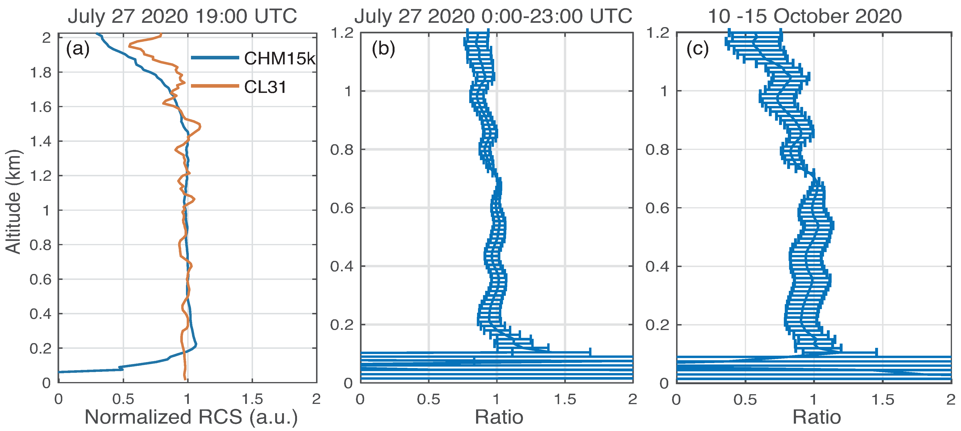
3.1. Near Range Signal Evaluation
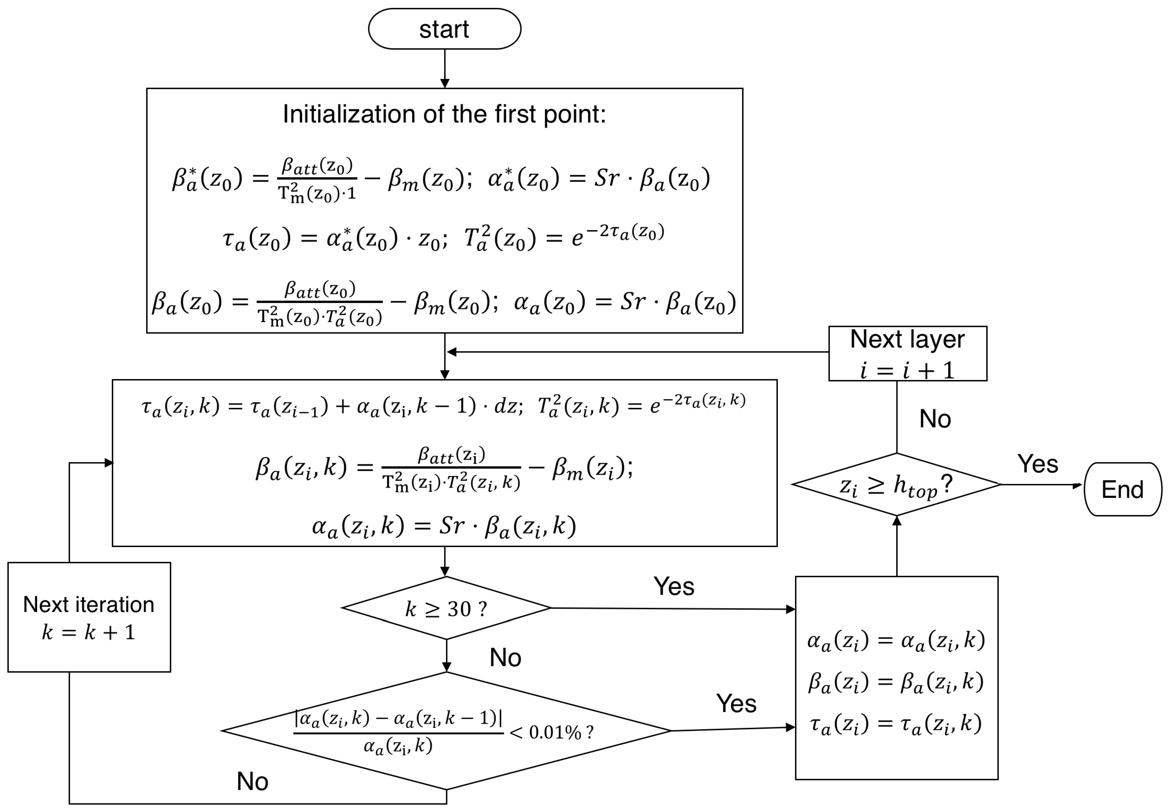
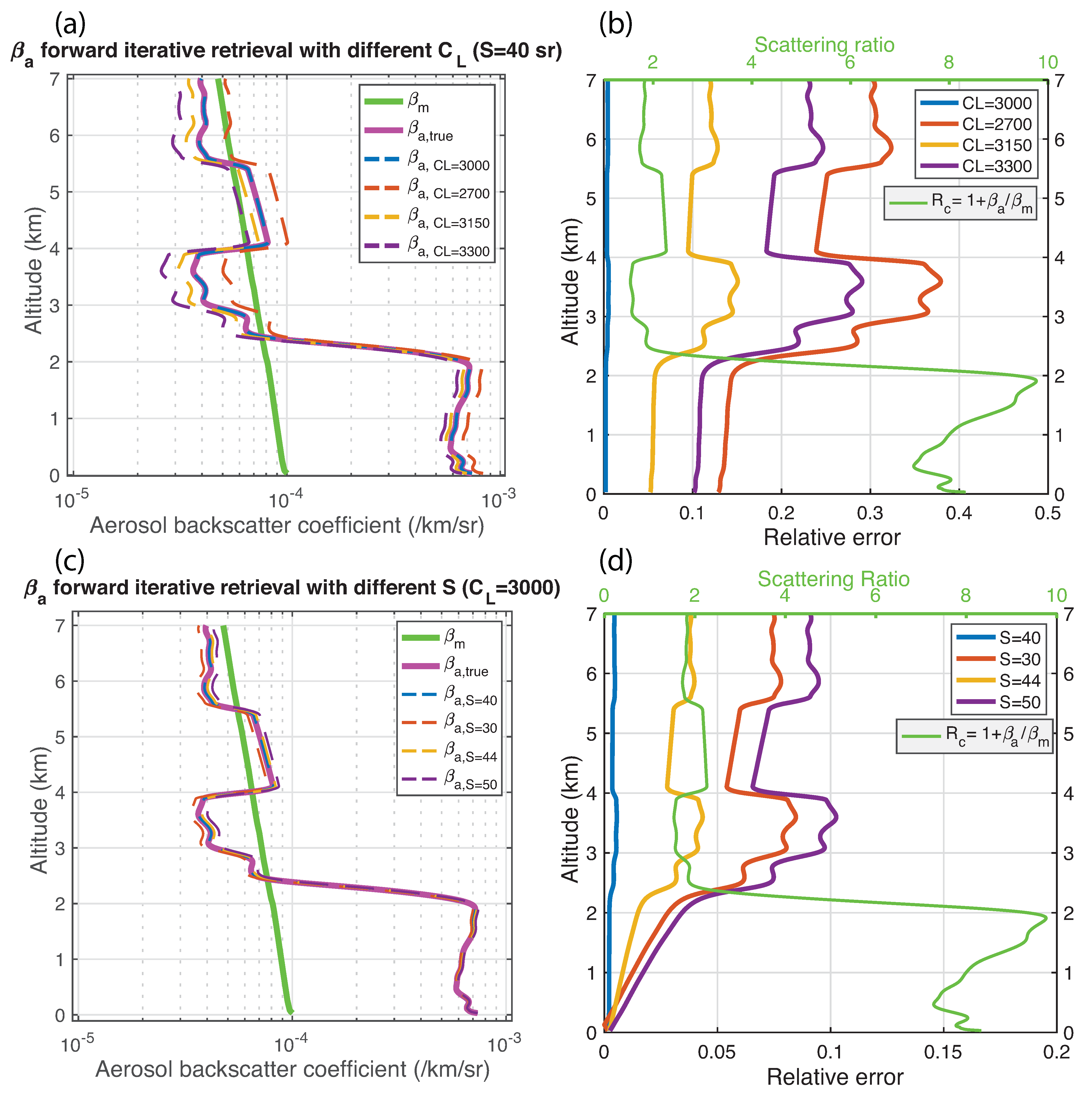
3.2. Aerosol Backscatter Retrieval with Forward Iterative Method
3.3. Calibration
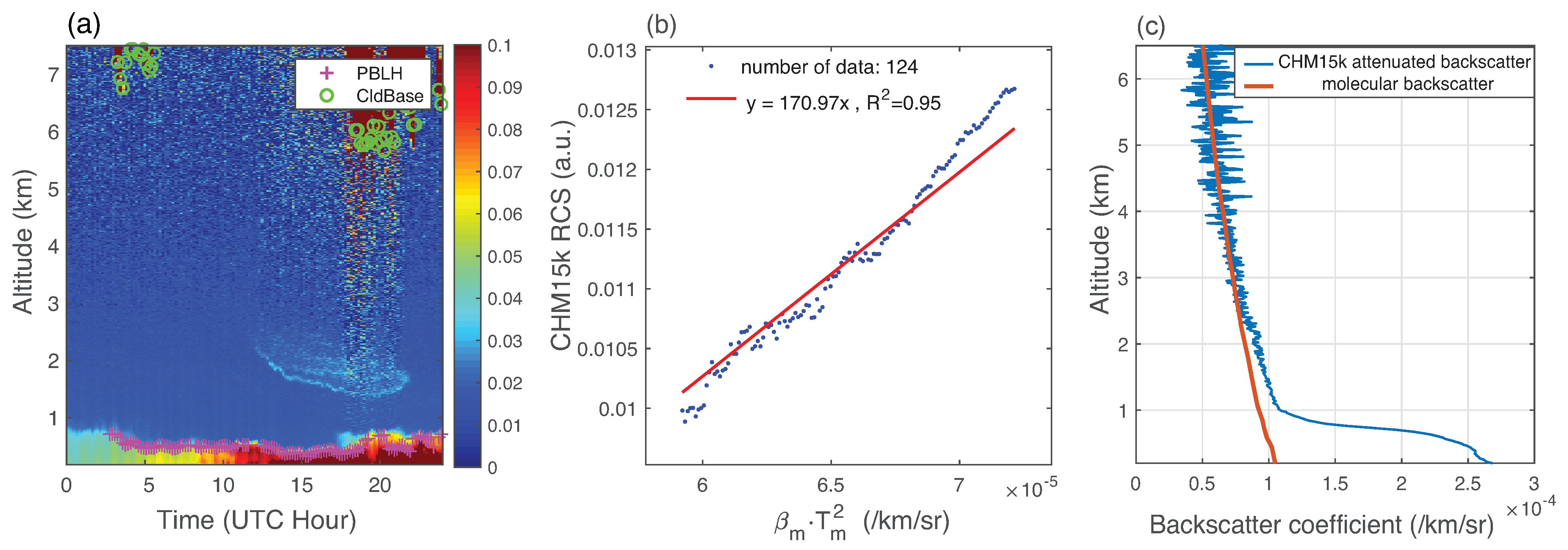
3.3.1. Rayleigh Calibration
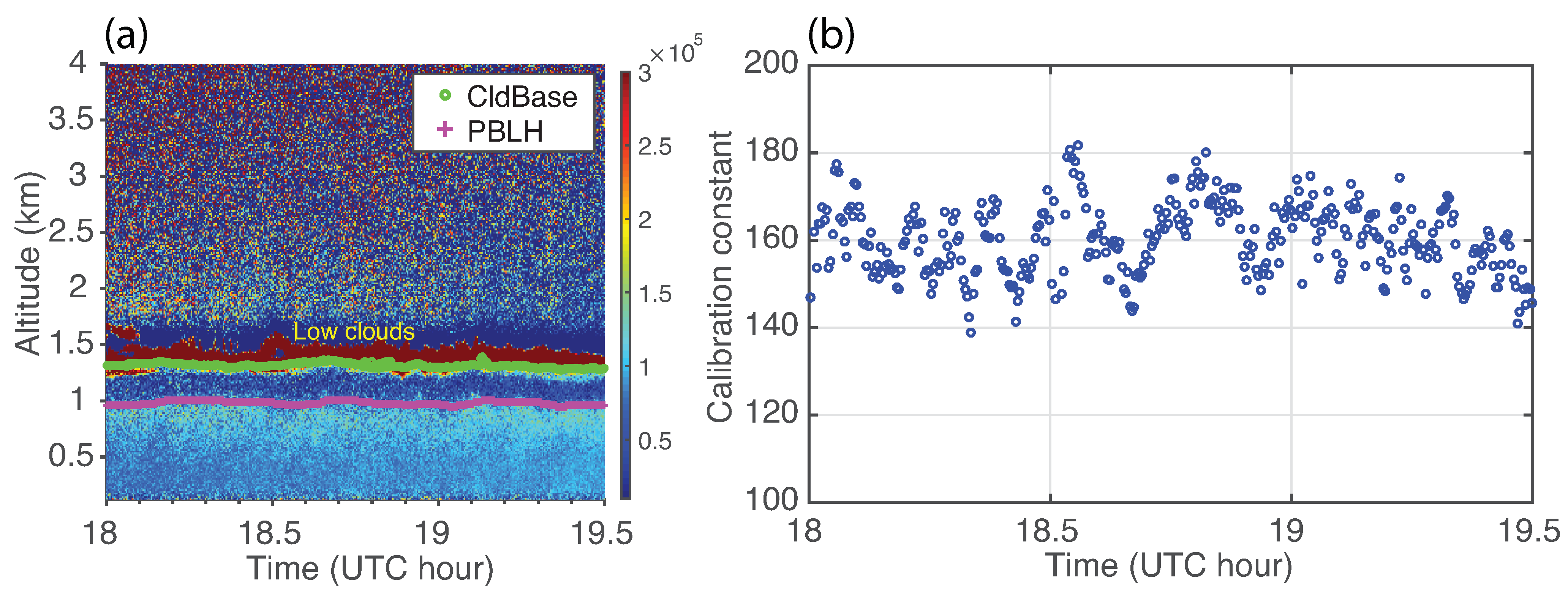
3.3.2. Liquid Cloud Calibration
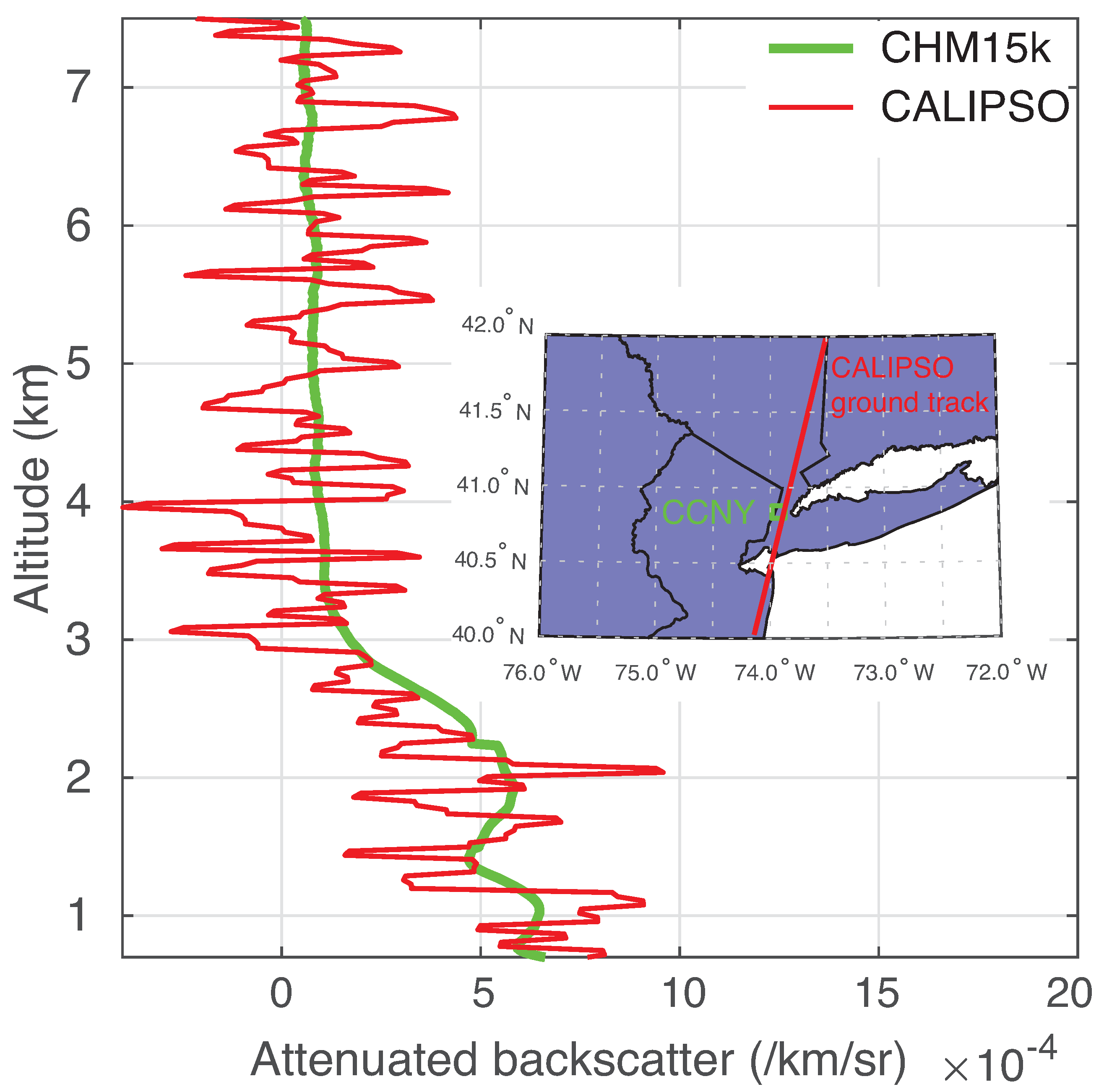
3.3.3. Comparison with CALIPSO Attenuated Backscatter Coefficient Profile
4. Results
4.1. Retrieval Results
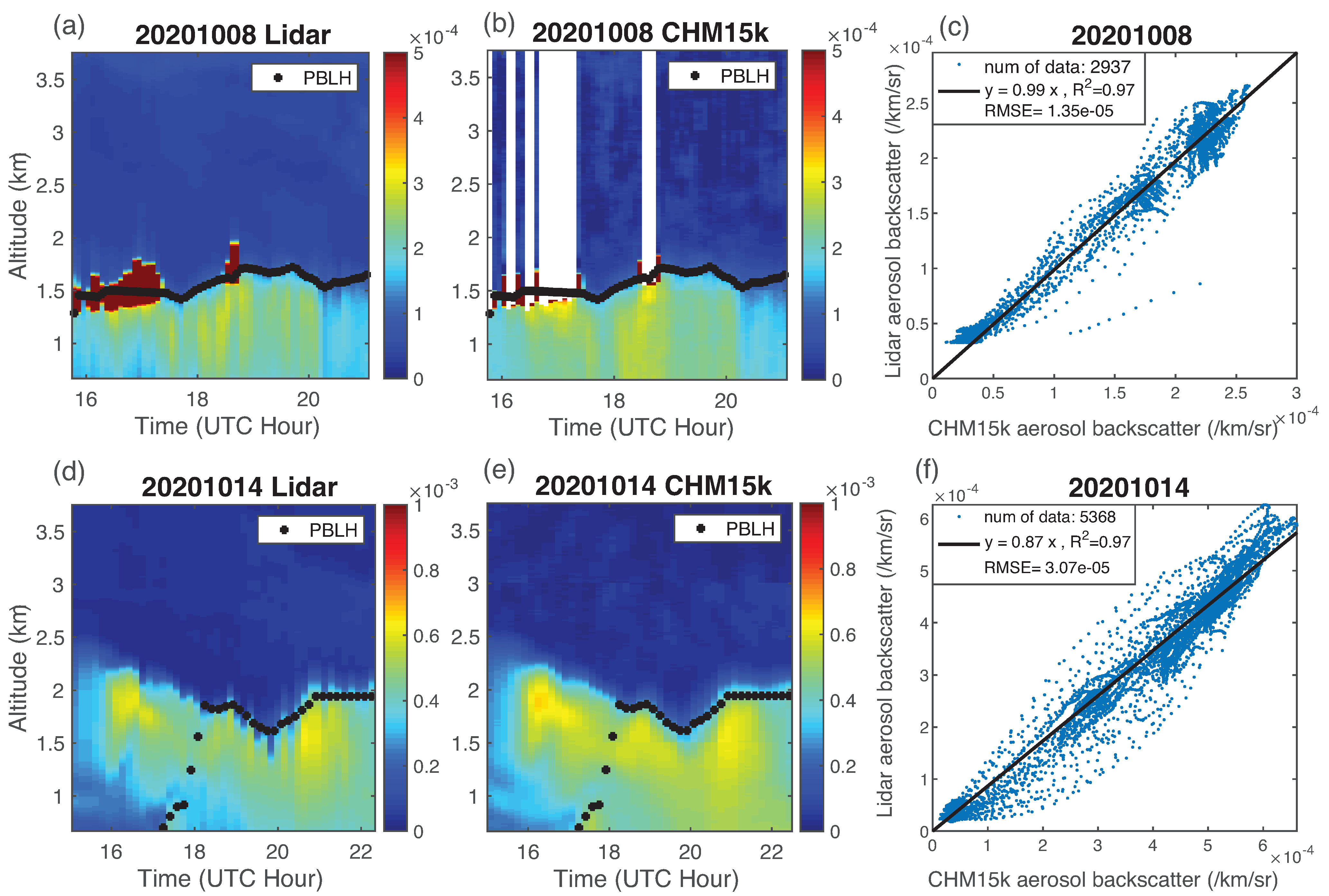
4.2. Evaluation
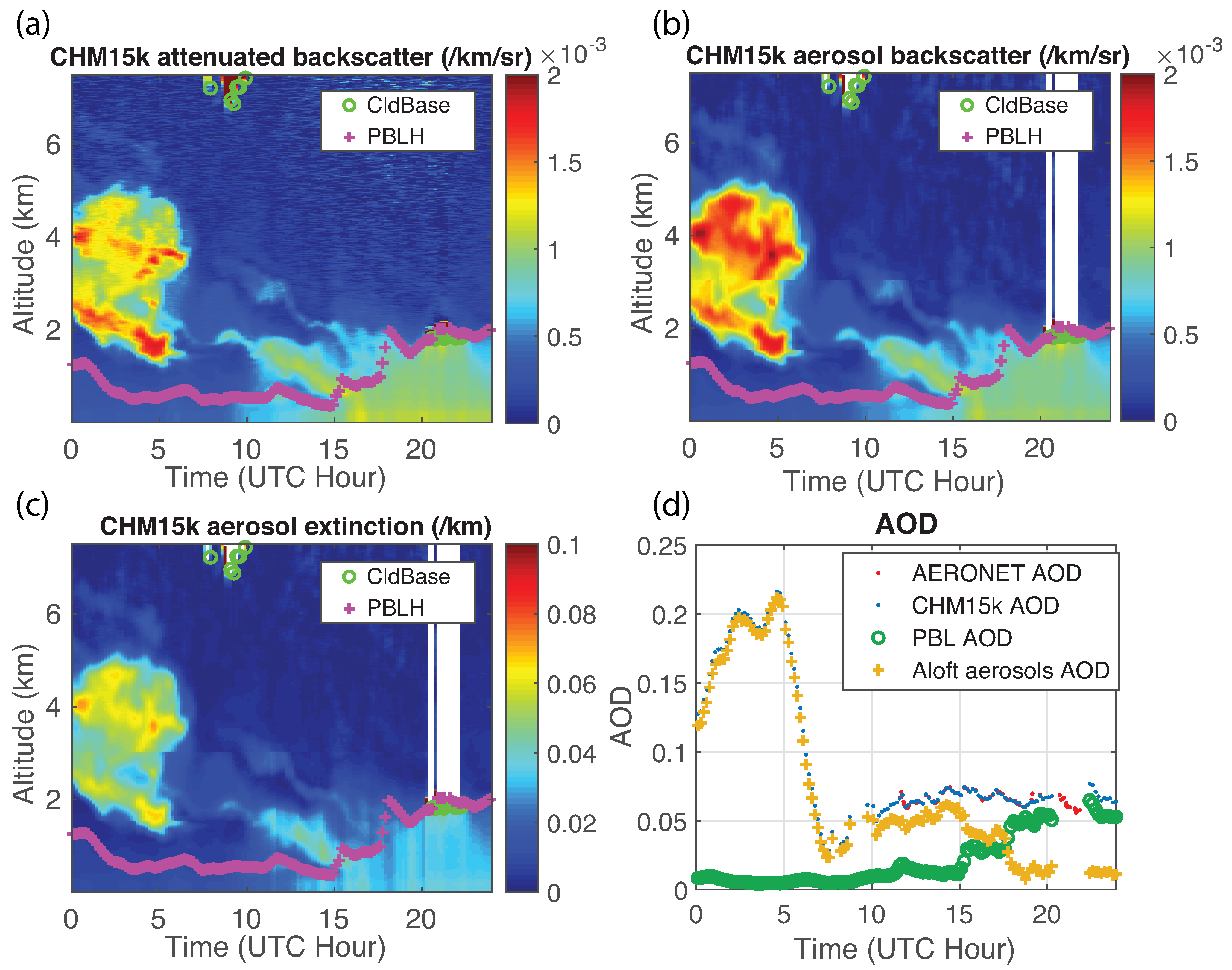
4.3. Application
5. Discussion
6. Conclusions
Author Contributions
Funding
Data Availability Statement
Acknowledgments
Conflicts of Interest
References
- Hicks, M.; Demoz, B.; Vermeesch, K.; Atkinson, D. Intercomparison of Mixing Layer Heights from the National Weather Service Ceilometer Test Sites and Collocated Radiosondes. J. Atmos. Ocean. Technol. 2019, 36, 129–137. [Google Scholar] [CrossRef] [Green Version]
- Wiegner, M.; Mattis, I.; Pattantyús-Ábrahám, M.; Bravo-Aranda, J.A.; Poltera, Y.; Haefele, A.; Hervo, M.; Görsdorf, U.; Leinweber, R.; Gasteiger, J.; et al. Aerosol backscatter profiles from ceilometers: Validation of water vapor correction in the framework of CeiLinEx2015. Atmos. Meas. Tech. 2019, 12, 471–490. [Google Scholar] [CrossRef] [Green Version]
- Haeffelin, M.; Angelini, F.; Morille, Y.; Martucci, G.; Frey, S.; Gobbi, G.P.; Lolli, S.; O’Dowd, C.D.; Sauvage, L.; Xueref-Rémy, I.; et al. Evaluation of Mixing-Height Retrievals from Automatic Profiling Lidars and Ceilometers in View of Future Integrated Networks in Europe. Bound.-Layer Meteorol. 2012, 143, 49–75. [Google Scholar] [CrossRef]
- Knepp, T.N.; Szykman, J.J.; Long, R.; Duvall, R.M.; Krug, J.; Beaver, M.; Cavender, K.; Kronmiller, K.; Wheeler, M.; Delgado, R.; et al. Assessment of mixed-layer height estimation from single-wavelength ceilometer profiles. Atmos. Meas. Tech. 2017, 10, 3963–3983. [Google Scholar] [CrossRef] [Green Version]
- Kotthaus, S.; Grimmond, C.S.B. Atmospheric boundary-layer characteristics from ceilometer measurements. Part 1: A new method to track mixed layer height and classify clouds. Q. J. R. Meteorol. Soc. 2018, 144, 1525–1538. [Google Scholar] [CrossRef] [Green Version]
- Kotthaus, S.; Grimmond, C.S.B. Atmospheric boundary-layer characteristics from ceilometer measurements. Part 2: Application to London’s urban boundary layer. Q. J. R. Meteorol. Soc. 2018, 144, 1511–1524. [Google Scholar] [CrossRef] [Green Version]
- Dang, R.; Yang, Y.; Hu, X.M.; Wang, Z.; Zhang, S. A review of techniques for diagnosing the atmospheric boundary layer height (ABLH) using aerosol lidar data. Remote Sens. 2019, 11, 1590. [Google Scholar] [CrossRef] [Green Version]
- Caicedo, V.; Delgado, R.; Sakai, R.; Knepp, T.; Williams, D.; Cavender, K.; Lefer, B.; Szykman, J. An Automated Common Algorithm for Planetary Boundary Layer Retrievals Using Aerosol Lidars in Support of the U.S. EPA Photochemical Assessment Monitoring Stations Program. J. Atmos. Ocean. Technol. 2020, 37, 1847–1864. [Google Scholar] [CrossRef]
- Kotthaus, S.; Haeffelin, M.; Drouin, M.A.; Dupont, J.C.; Grimmond, S.; Haefele, A.; Hervo, M.; Poltera, Y.; Wiegner, M. Tailored algorithms for the detection of the atmospheric boundary layer height from common automatic lidars and ceilometers (Alc). Remote Sens. 2020, 12, 3259. [Google Scholar] [CrossRef]
- Chan, K.L.; Wiegner, M.; Flentje, H.; Mattis, I.; Wagner, F.; Gasteiger, J.; Geiß, A. Evaluation of ECMWF-IFS (version 41R1) operational model forecasts of aerosol transport by using ceilometer network measurements. Geosci. Model Dev. 2018, 11, 3807–3831. [Google Scholar] [CrossRef] [Green Version]
- Hoff, R.M.; Christopher, S.A. Remote Sensing of Particulate Pollution from Space: Have We Reached the Promised Land? J. Air Waste Manag. Assoc. 2009, 59, 645–675. [Google Scholar] [CrossRef]
- Liu, Y.; Wang, Z.; Wang, J.; Ferrare, R.A.; Newsom, R.K.; Welton, E.J. The effect of aerosol vertical profiles on satellite-estimated surface particle sulfate concentrations. Remote Sens. Environ. 2011, 115, 508–513. [Google Scholar] [CrossRef] [Green Version]
- Münkel, C.; Eresmaa, N.; Räsänen, J.; Karppinen, A. Retrieval of mixing height and dust concentration with lidar ceilometer. Bound.-Layer Meteorol. 2007, 124, 117–128. [Google Scholar] [CrossRef]
- Wiegner, M.; Madonna, F.; Binietoglou, I.; Forkel, R.; Gasteiger, J.; Geiß, A.; Pappalardo, G.; Schäfer, K.; Thomas, W. What is the benefit of ceilometers for aerosol remote sensing? An answer from EARLINET. Atmos. Meas. Tech. 2014, 7, 1979–1997. [Google Scholar] [CrossRef] [Green Version]
- Jin, Y.; Sugimoto, N.; Shimizu, A.; Nishizawa, T.; Kai, K.; Kawai, K.; Yamazaki, A.; Sakurai, M.; Wille, H. Evaluation of ceilometer attenuated backscattering coefficients for aerosol profile measurement. J. Appl. Remote Sens. 2018, 12, 042604. [Google Scholar] [CrossRef]
- Wiegner, M.; Geiß, A. Aerosol profiling with the JenOptik ceilometer CHM15kx. Atmos. Meas. Tech. 2012, 5, 1953–1964. [Google Scholar] [CrossRef] [Green Version]
- Wu, Y.; Gan, C.M.; Cordero, L.; Gross, B.; Moshary, F.; Ahmed, S. Calibration of the 1064 nm lidar channel using water phase and cirrus clouds. Appl. Opt. 2011, 50, 3987. [Google Scholar] [CrossRef] [PubMed]
- O’Connor, E.J.; Illingworth, A.J.; Hogan, R.J. A Technique for Autocalibration of Cloud Lidar. J. Atmos. Ocean. Technol. 2004, 21, 10. [Google Scholar] [CrossRef]
- Li, S.; Joseph, E.; Min, Q. Remote sensing of ground-level PM2.5 combining AOD and backscattering profile. Remote Sens. Environ. 2016, 183, 120–128. [Google Scholar] [CrossRef]
- Li, D.; Gross, B.; Wu, Y.; Moshary, F. Correlation Study of Planetary-Boundary-Layer-Height Retrievals from CL51 and CHM15K Ceilometers with Application To PM2.5 Dynamics in New York City. EPJ Web Conf. 2020, 237, 03010. [Google Scholar] [CrossRef]
- Klett, J.D. Stable analytical inversion solution for processing lidar returns. Appl. Opt. 1981, 20, 211. [Google Scholar] [CrossRef] [PubMed] [Green Version]
- Fernald, F.G. Analysis of atmospheric lidar observations: Some comments. Appl. Opt. 1984, 23, 652. [Google Scholar] [CrossRef] [PubMed]
- Binietoglou, I.; Amodeo, A.; D’Amico, G.; Giunta, A.; Madonna, F.; Mona, L.; Pappalardo, G. Examination of possible synergy between lidar and ceilometer for the monitoring of atmospheric aerosols. In Proceedings of the Lidar Technologies, Techniques, and Measurements for Atmospheric Remote Sensing VII. International Society for Optics and Photonics, San Diego, CA, USA, 1–5 August 2011; Volume 8182, p. 818209. [Google Scholar] [CrossRef]
- Madonna, F.; Amato, F.; Vande Hey, J.; Pappalardo, G. Ceilometer aerosol profiling versus Raman lidar in the frame of the INTERACT campaign of ACTRIS. Atmos. Meas. Tech. 2015, 8, 2207–2223. [Google Scholar] [CrossRef] [Green Version]
- Hopkin, E.; Illingworth, A.J.; Charlton-Perez, C.; Westbrook, C.D.; Ballard, S. A robust automated technique for operational calibration of ceilometers using the integrated backscatter from totally attenuating liquid clouds. Atmos. Meas. Tech. 2019, 12, 4131–4147. [Google Scholar] [CrossRef] [Green Version]
- Heese, B.; Flentje, H.; Althausen, D.; Ansmann, A.; Frey, S. Ceilometer lidar comparison: Backscatter coefficient retrieval and signal-to-noise ratio determination. Atmos. Meas. Tech. 2010, 3, 1763–1770. [Google Scholar] [CrossRef] [Green Version]
- Munkel, C.; Rasanen, J. New optical concept for commercial lidar ceilometers scanning the boundary layer. In Proceedings of the Remote Sensing of Clouds and the Atmosphere IX. International Society for Optics and Photonics, Bellingham, WA, USA, 9–13 April 2004; Volume 5571. [Google Scholar] [CrossRef]
- Martucci, G.; Milroy, C.; O’Dowd, C.D. Detection of Cloud-Base Height Using Jenoptik CHM15K and Vaisala CL31 Ceilometers. J. Atmos. Ocean. Technol. 2010, 27, 305–318. [Google Scholar] [CrossRef]
- Wu, Y.; Chaw, S.; Gross, B.; Moshary, F.; Ahmed, S. Low and optically thin cloud measurements using a Raman-Mie lidar. Appl. Opt. 2009, 48, 1218–1227. [Google Scholar] [CrossRef] [PubMed]
- Holben, B.; Eck, T.; Slutsker, I.; Tanré, D.; Buis, J.; Setzer, A.; Vermote, E.; Reagan, J.; Kaufman, Y.; Nakajima, T.; et al. AERONET—A Federated Instrument Network and Data Archive for Aerosol Characterization. Remote Sens. Environ. 1998, 66, 1–16. [Google Scholar] [CrossRef]
- Sinyuk, A.; Holben, B.N.; Eck, T.F.; Giles, D.M.; Slutsker, I.; Korkin, S.; Schafer, J.S.; Smirnov, A.; Sorokin, M.; Lyapustin, A. The AERONET Version 3 aerosol retrieval algorithm, associated uncertainties and comparisons to Version 2. Atmos. Meas. Tech. 2020, 13, 3375–3411. [Google Scholar] [CrossRef]
- Kotthaus, S.; O’Connor, E.; Münkel, C.; Charlton-Perez, C.; Haeffelin, M.; Gabey, A.M.; Grimmond, C.S.B. Recommendations for processing atmospheric attenuated backscatter profilesfrom Vaisala CL31 ceilometers. Atmos. Meas. Tech. 2016, 9, 3769–3791. [Google Scholar] [CrossRef] [Green Version]
- Platt, C.M.R. Lidar and Radiometric Observations of Cirrus Clouds. J. Atmos. Sci. 1973, 30, 1191–1204. [Google Scholar] [CrossRef] [Green Version]
- Pinnick, R.G.; Jennings, S.G.; Chýlek, P.; Ham, C.; Grandy, W.T. Backscatter and extinction in water clouds. J. Geophys. Res. 1983, 88, 6787. [Google Scholar] [CrossRef] [Green Version]
- Vaughan, M.; Garnier, A.; Josset, D.; Avery, M.; Lee, K.P.; Liu, Z.; Hunt, W.; Pelon, J.; Hu, Y.; Burton, S.; et al. CALIPSO lidar calibration at 1064 nm: Version 4 algorithm. Atmos. Meas. Tech. 2019, 12, 51–82. [Google Scholar] [CrossRef] [Green Version]
- Anderson, T.L.; Charlson, R.J.; Winker, D.M.; Ogren, J.A.; Holmén, K. Mesoscale variations of tropospheric aerosols. J. Atmos. Sci. 2003, 60, 119–136. [Google Scholar] [CrossRef]
- Pappalardo, G.; Wandinger, U.; Mona, L.; Hiebsch, A.; Mattis, I.; Amodeo, A.; Ansmann, A.; Seifert, P.; Linné, H.; Apituley, A.; et al. EARLINET correlative measurements for CALIPSO: First intercomparison results. J. Geophys. Res. Atmos. 2010, 115. [Google Scholar] [CrossRef] [Green Version]


| Date (mm/dd/yy) | System Constant (kmsr) | Correlation | Range (km) | Number of Data Points | Radio-Sound Time (UTC) | Profile Time (UTC) |
|---|---|---|---|---|---|---|
| 12/19/18 | 170.97 | 0.95 | 3.2–5.0 | 124 | 0:00 | 00:00–04:00 |
| 12/20/18 | 177.56 | 0.98 | 3.0–5.0 | 134 | 0:00 | 00:00–04:00 |
| 01/04/19 | 171.21 | 0.95 | 4.0–5.5 | 101 | 12:00 | 06:00–11:00 |
| 01/22/19 | 169.43 | 0.98 | 3.0–6.0 | 201 | 12:00 | 06:00–11:00 |
| 02/01/19 | 163.7 | 0.96 | 3.9–5.0 | 74 | 0:00 | 00:00–04:00 |
| 02/04/19 | 171.01 | 0.92 | 3.5–5.5 | 135 | 0:00 | 00:00–04:00 |
| 12/12/19 | 152.85 | 0.97 | 3.5–6.5 | 201 | 12:00 | 05:00–11:00 |
| 12/21/19 | 152.57 | 0.96 | 2.5–4.5 | 134 | 0:00 | 00:00–04:00 |
| 12/21/19 | 152.58 | 0.91 | 3.5–5.4 | 128 | 12:00 | 06:00–11:00 |
| 12/23/19 | 147.24 | 0.95 | 2.7–4.2 | 101 | 0:00 | 00:00–04:00 |
| 01/30/20 | 150.42 | 0.92 | 3.0–5.0 | 134 | 12:00 | 06:00–11:00 |
Publisher’s Note: MDPI stays neutral with regard to jurisdictional claims in published maps and institutional affiliations. |
© 2021 by the authors. Licensee MDPI, Basel, Switzerland. This article is an open access article distributed under the terms and conditions of the Creative Commons Attribution (CC BY) license (https://creativecommons.org/licenses/by/4.0/).
Share and Cite
Li, D.; Wu, Y.; Gross, B.; Moshary, F. Capabilities of an Automatic Lidar Ceilometer to Retrieve Aerosol Characteristics within the Planetary Boundary Layer. Remote Sens. 2021, 13, 3626. https://doi.org/10.3390/rs13183626
Li D, Wu Y, Gross B, Moshary F. Capabilities of an Automatic Lidar Ceilometer to Retrieve Aerosol Characteristics within the Planetary Boundary Layer. Remote Sensing. 2021; 13(18):3626. https://doi.org/10.3390/rs13183626
Chicago/Turabian StyleLi, Dingdong, Yonghua Wu, Barry Gross, and Fred Moshary. 2021. "Capabilities of an Automatic Lidar Ceilometer to Retrieve Aerosol Characteristics within the Planetary Boundary Layer" Remote Sensing 13, no. 18: 3626. https://doi.org/10.3390/rs13183626
APA StyleLi, D., Wu, Y., Gross, B., & Moshary, F. (2021). Capabilities of an Automatic Lidar Ceilometer to Retrieve Aerosol Characteristics within the Planetary Boundary Layer. Remote Sensing, 13(18), 3626. https://doi.org/10.3390/rs13183626