Hyperspectral Image Classification Based on Sparse Superpixel Graph

Abstract

Hyperspectral image (HSI) classification is one of the major problems in the field of remote sensing. Particularly, graph-based HSI classification is a promising topic and has received increasing attention in recent years. However, graphs with pixels as nodes generate large size graphs, thus increasing the computational burden. Moreover, satisfactory classification results are often not obtained without considering spatial information in constructing graph. To address these issues, this study proposes an efficient and effective semi-supervised spectral-spatial HSI classification method based on sparse superpixel graph (SSG). In the constructed sparse superpixels graph, each vertex represents a superpixel instead of a pixel, which greatly reduces the size of graph. Meanwhile, both spectral information and spatial structure are considered by using superpixel, local spatial connection and global spectral connection. To verify the effectiveness of the proposed method, three real hyperspectral images, Indian Pines, Pavia University and Salinas, are chosen to test the performance of our proposal. Experimental results show that the proposed method has good classification completion on the three benchmarks. Compared with several competitive superpixel-based HSI classification approaches, the method has the advantages of high classification accuracy (>97.85%) and rapid implementation (<10 s). This clearly favors the application of the proposed method in practice.

1. Introduction

Although continuous development of hyperspectral sensors makes it easy to collect a large amount of hyperspectral data, labeling the acquired data is expensive [1]. As a result of this fact, semi-supervised hyperspectral image (HSI) classification methods have been extensively investigated in the past decades [2,3,4,5]. In turn, the successful application of HSI classification in urban mapping [6], environment monitoring [7], precision agriculture [8] and other fields promotes the improvement of classification methods. Currently, it still remains an issue worthy of further study to develop new semi-supervised methods to classify an HSI fast and accurately, due to its characteristics of big data [9,10].

Unlike big data recorded in other fields, one of the remarkable features of hyperspectral data is that it clearly contains spatial structure information in addition to spectral information. This means that classification results may be improved by integrating spatial and spectral information based on classification techniques or classifier. Satisfactory classification results of plenty of existing spectral-spatial HSI classification methods have demonstrated the feasibility of this integration [11,12,13,14,15,16]. Using fixed-size window technique, the methods of Markov random field [17], guided filter [18], discontinuity preserving relaxation [19,20], and recursive filtering [21] successfully adopted spatial information to smooth the noisy pixels contained in the HSI. The use of these smoothing techniques in classification results in an effective reduction in the number of misclassified pixels. In multiple kernels-based classification methods, the spatial and spectral information was effectively fused by using composite kernels to enhance the classification of hyperspectral images [22,23]. The spatial structure information was also used to correct some misclassified pixels in the classification map by majority voting rule [24,25]. Multi-scale covariance maps were introduced to solve the overfitting problem of convolutional neural network-based methods in HSI classification [26]. Additionally, the existing works show that in the classification process, the combination of spatial information with dimensionality reduction [27], sparse representation [28,29], low rank representation [30], convolutional neural network [31] and various techniques do contribute to improving the classification accuracy.

Among a mass of spectral-spatial HSI classification methods, the superpixel-based approach is a representative method and has been extensively investigated in recent years because superpixels are homogeneous and adaptive in size and shape [32,33,34,35]. Compared with fixed-size window, the adaptive size and shape are more favorable to explore the spectral and spatial relationships in HSI classification. Based on superpixels and multi-view active learning, an HSI classification method was proposed, aiming at improving the classification performance and reducing the manual labeling effort [36]. Under the assumption of superpixel homogeneity, a series of superpixel-level HSI classification methods have been introduced in recent years [34,37,38,39,40]. Xie et al. [37] developed a semi-supervised spectral-spatial classification approach at the superpixel-level by the improved simple linear iterative clustering and k-nearest neighbor classifier. Using k-nearest neighbor rules twice, Tu et al. [39] defined the distance between superpixels to explore the optimal representations of superpixels and then suggested a superpixel-level HSI classifier. One of the advantages of superpixel-level classifier is to quickly implement the classification process through reducing an HSI from the aspect of pixels. However, the adaptive size and shape feature of superpixels makes it arduous to measure the similarity between superpixels. Therefore, although there are many superpixel-based classification methods, few works are dedicated to superpixel-level classification algorithms.

A great deal of work has shown that graph is a powerful tool in the fields of machine learning, computer vision and remote sensing, due to its surprisingly flexible representation ability [41,42,43,44,45]. By means of graph theory, label propagation rule or complex network theory, HSI classification is successfully transformed into a graph partition in graph-based HSI classification methods. Camps-Valls et al. early suggested a semi-supervised graph-based classifier specifically designed for processing hyperspectral images [46]. Based on superpixels and a spectral–spatial sparse graph, a semi-supervised adaptive label propagation algorithm was depicted to address the pollution of label information by random noise and boundary noise [47]. Using the spectral and spatial information extracted from superpixels, Sellars et al. [40] constructed a weighted superpixel graph, where each vertex represents a superpixel. Then a graph-based semi-supervised HSI classification framework was proposed. Recently, graph convolutional network (GCN) schemes and its various improvements have been proposed to classify HSI [48,49,50,51]. GCN adopts graph to carry out the convolution on arbitrarily structured non-Euclidean data to improve the classification performances of convolutional neural network with fixed size and weight convolution kernel. In these graph-based HSI classification methods, various techniques for constructing and partitioning graphs were adopted to achieve accurate classification of HSI. In general, the performance of graph-based classification methods relies on the construction and division of graphs. It is known that superpixel graphs usually have smaller sizes than those with pixels as vertices. This means that for the same label propagation on graph algorithm, it will take less time to complete the classification task. Therefore, it is interesting to further develop novel superpixel graphs based HSI classification methods.

The applications of discrete potential theory on graphs have been previously investigated in various fields, such as image segmentation [52], text data classification [53], community structure detection [54] and so on. Motivated by random walks and based on discrete potential theory, Grady proposed a novel algorithm for image segmentation [52]. An effective semi-supervised algorithm was developed to detect the community structure in complex networks through discrete potential theory [54]. The potential theory on directed graph was discussed to discover factors of the network formation [55]. The difference between different applications makes it meaningful to further extend this theory to more fields, especially to remote sensing.

Inspired by the works on superpixel-level classifier, label propagation on graph and discrete potential theory, in this work, a novel superpixel graph-based scheme is proposed to classify HSI efficiently. In this proposal, a novel and computationally simple distance is first defined to measure the similarity of two superpixels. A sparse superpixel graph (with superpixels as vertices) is then constructed by local spatial connection and global spectral connection. Based on the constructed superpixel graph and discrete potential theory, the HSI classification is converted into an optimization problem that can be solved by a system of linear algebraic equations. We here adopt the conjugate gradient descent method (CGDM) to find the approximate solution because of its rapid convergence and strong robustness. Finally, according to the greatest potential of each vertex computed by the CGDM, superpixels can be properly labeled. A range of experimental and comparative results on three benchmarks extensively validate our scheme.

The main technical contributions of the proposal include:

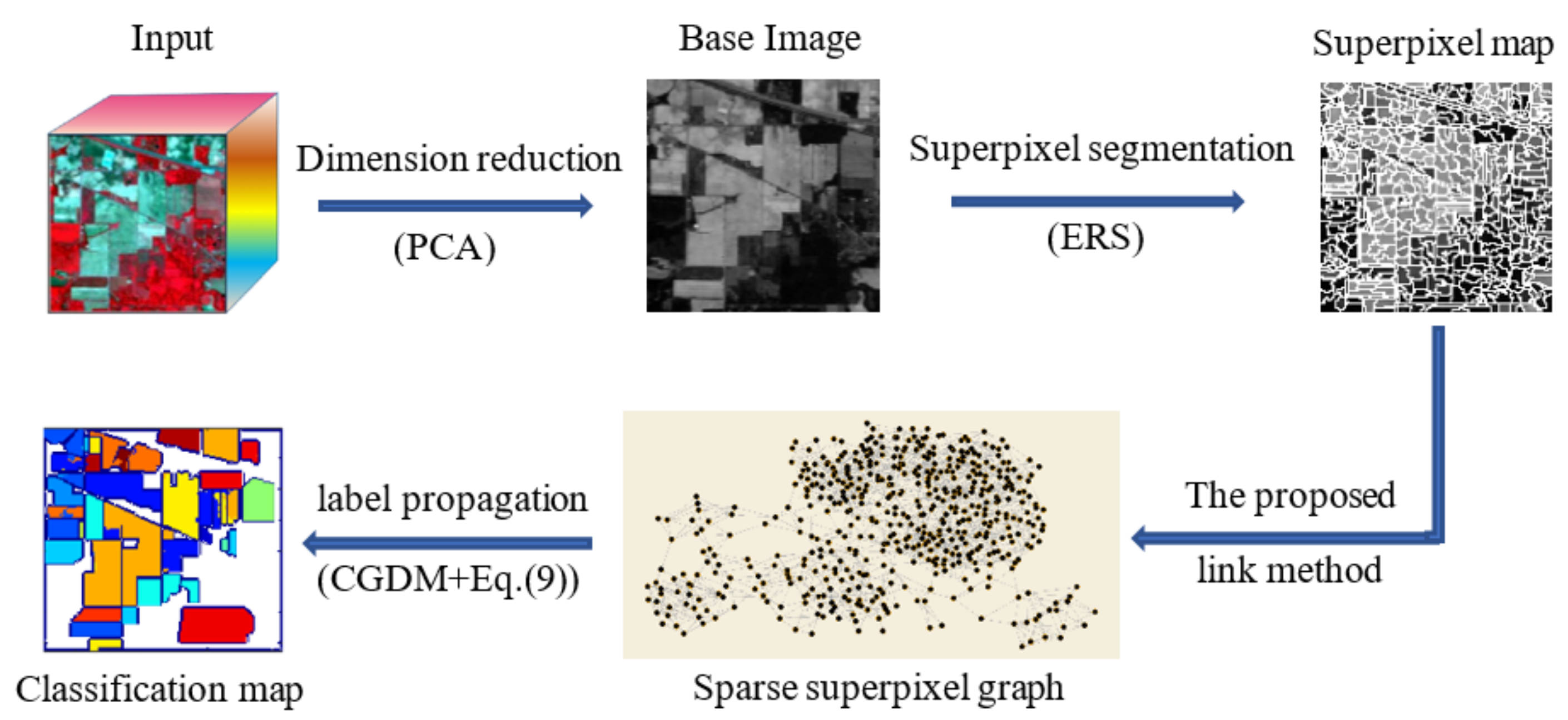
• An efficient HSI classification scheme is suggested based on sparse superpixel graph.
• A computationally simple but effective distance between superpixels is newly defined.
• A sparse superpixel graph is constructed by using spectral-spatial connection strategy.
• The use of CGDM in the proposal speeds up the process of label propagation on graph.

The rest of this paper is organized as follows: Section 2 details the process of the proposed method, including superpixel segmentation, the new definition of distance between superpixels, the construction of sparse superpixel graph and label propagation on graph. Experimental and comparative results are reported in Section 3. Section 4 analyzes the influence of the parameters used in our method. Finally, discussions and conclusions are given in Section 5 and Section 6.

2. Methods

In this section, we describe the proposed method in detail. The classification framework includes dimension reduction, superpixel segmentation, construction of sparse superpixel graph and label propagation on graph, as shown in Figure 1.

2.1. Superpixel Segmentation

Superpixel segmentation is often understood as the problem of region localization of an image. Generally, the number of pixels contained in each superpixel is automatically generated in terms of local image structure by using superpixel segmentation algorithms. Thus, different superpixels may have different shapes. These adaptive features of superpixels are obviously propitious to good homogeneity of the generated superpixels.

Among many segmentation algorithms, the graph-based entropy rate superpixel segmentation (ERS) [56] is commonly used in remote sensing because of its excellent performance in good effectiveness and high efficiency. However, the high-dimension property of hyperspectral data does not allow to divide an HSI into superpixels by using classical ERS straightly. Therefore, we need to execute principal component analysis approach in advance and take the first principal component to generate the base image used for segmentation.

The ERS method is an optimization algorithm based on edge clustering. For user-defined number of superpixel p and a set of edges M, the ERS approach splits the base image into superpixels through optimizing the following objective function with restrict conditions according to set M [56]:

$$\{\begin{array}{c}\underset{\mathrm{M}}{max}\left(\mathrm{R}\left(\mathrm{M}\right)+\omega \mathrm{B}\left(\mathrm{M}\right)\right)\\ subject\\ \end{array}\mathrm{M}\subseteq \mathrm{E}\wedge N_{\mathrm{M}}\ge p,|$$

(1)

where R(M) and B(M) are entropy rate term and balancing term, respectively. N_M indicates the number of the obtained superpixels; $\omega$ is a balancing parameter, and E is an edge set.

In Equation (1), the introduction of entropy rate term is to include spatial neighbor pixels with similar spectral information as much as possible in a superpixel. However, this may cause significant differences in superpixel size. The use of the balance term and balancing parameter effectively avoids this phenomenon. Interested readers can consult with Liu’s work for more details of ERS method [56].

2.2. Distance between Superpixels

It is one of the key issues to properly define the distance between superpixels in the superpixel-level HSI methods. A desired distance should not only better measure the intimate relationship between two superpixels but also should be computationally simple. However, this is a nontrivial task because superpixels have different sizes. In [34,37,38,39,40], the distance/similarity of a pair of superpixels was defined by using various techniques. Although the similarity of two superpixels can be better measured by these designed distances, it is time-consuming to calculate them.

To address this problem, a simple but effective distance between superpixels is defined in this work. In the suggested distance, we carefully consider the statistical features of a superpixel, that is, mean, median and mode. Specifically, for a generated superpixels $S_i$ containing $n_i$ pixels, we first construct the mean vector ${\alpha }_1^i$, the median vector ${\alpha }_2^i$ and the mode vector ${\alpha }_3^i$ by orderly computing the mean, the median and the mode of each band of these $n_i$ pixels. The superpixel $S_i$ is then approximately represented by a newly defined sample with the same dimension as the original HSI,

$${\alpha }_i=w_1{\alpha }_1^i+w_2{\alpha }_2^i+\left(1-w_1-w_2\right){\alpha }_3^i$$

(2)

where $w_1$ and $w_2$ are the weights that control the importance of each component.

Finally, a novel distance between superpixels $S_i$ and $S_j$ can be defined as

$$d(S_i,S_j)=d({\alpha }_i,{\alpha }_j)=\sqrt{{{\displaystyle \sum }}_{h=1}^B{\left({\alpha }_{i,h}-{\alpha }_{j,h}\right)}^2}.$$

(3)

where $B$ is the number of bands.

In Equation (3), distance between the vectors ${\alpha }_i$ and ${\alpha }_j$ may choose the desired distance, for example, the commonly used Euclidean distance. Furthermore, the adoption of the median vector and the mode vector in Equation (2) effectively reduces the impact of noise pixels on distance computation. The advantage of the distance defined here is simple to calculate because it is independent of the shape and size of the superpixels. The validity of the above definition has been widely verified in the experiments carried out in this work.

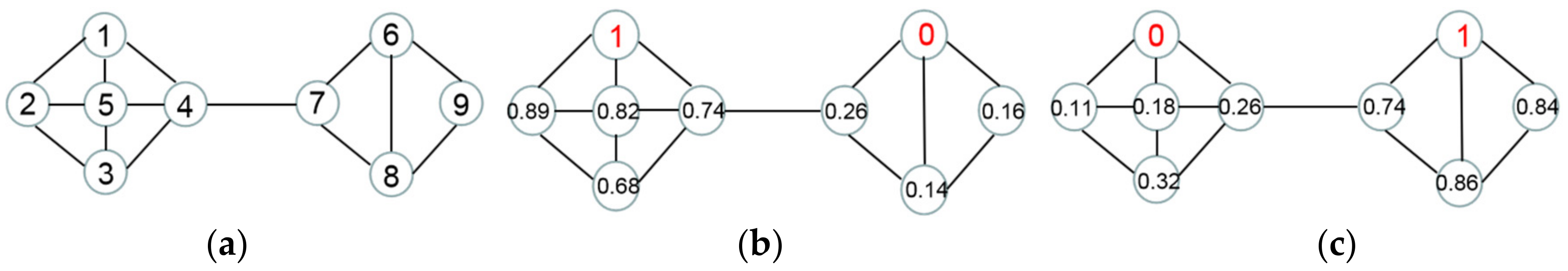
2.3. The Construction of Sparse Superpixel Graph

A majority of existing work on HSI classification demonstrates that the graph-based methods have a promising future, partially due to amazing data presentation ability of graphs. In the field of remote sensing, a vertex of the graphs may represent a pixel or a superpixel. We term a graph as a superpixel graph if the vertices in a graph represent superpixels. It is clear that superpixel graph has a smaller size than the one with pixels as vertices. This means that it is possible to take less time to partition a graph. Considering this advantage of superpixel graph, we use a superpixel graph to represent an HSI for classification.

It is known that there is abundant spatial information in a given HSI, besides rich spectral information. Notably, the effective fusion of spectral and spatial information is helpful to improve the classification results. Therefore, we adopt the method of global spectral connection and local spatial connection to construct desired superpixel graph by using KNN rule twice.

During the spectral connection, we firstly calculate the distances of the superpixel $S_i$ to the rest according to Equation (3), and then arrange them in an ascending order. For user-specified $k_1$, we finally connect the superpixel $S_i$ to its first $k_1$ superpixels. In this stage, we only consider the spectral information of superpixels and search the nearest neighbors of the superpixel in a global range. This connection approach attempts to deal with the problem that the superpixels belonging to the same class are disconnected or far from each other in space.

In the process of local connection, for each superpixel, one connects it to $k_2$ nearest neighbors in all its spatial adjacent superpixels in terms of Equation (3). This link strategy aims to maintain local consistency by density connections.

The constructed graph is an efficient combination of spectral-based graph and spatial-based graph. Please note that a superpixel may be linked twice in global and local connections. It has no effect on the constructed superpixel graph because we only record the link regardless of the number of links.

The superpixel graph constructed here is an unweighted and undirected sparse graph. This provides the basis to predict the classes of label-free vertices using a variety of classical or popular label propagation techniques. In next subsection, we would like to use the discrete potential theory and conjugate gradient descent algorithm to predict the class of each unlabeled vertex in the constructed graph.

Let G = (V, E) be the constructed superpixel graph, where $\mathrm{V}=\left\{v_1,v_2,\cdots ,v_p\right\}$ is the set of vertices and $\mathrm{E}\subseteq \mathrm{V}\times \mathrm{V}$ is the collection of edges. Commonly, we use an adjacent matrix A to describe the graph G, where the element $a_{i,j}$ of A is equal to 1 if there is an edge between vertices $v_i$ and $v_j$ and 0 otherwise.

The Laplace matrix of graph G is usually defined as

$$\mathrm{L}=\mathrm{D}-\mathrm{A},$$

(4)

where the diagonal matrix D is the degree matrix of A. The matrix L is obviously symmetry and positive semi-definite.

2.4. Label Propagation on Graph

A graph can be regarded as an electrostatic field if one or more vertices are assigned to an electric potential 1 and some vertices to 0. Particularly, the electrostatic field is termed as m-label generation if we assign an unit potential to the vertices with label m and zero to other labeled vertices with class label rather than m. This electrostatic field is simply denoted by m-EF. The potentials of the reminding unlabeled vertices can be calculated by solving a system of linear algebraic equations derived from combinatorial Dirichlet problem with the boundary conditions [52]. In this sense, the process of potential transmission in the electrostatic field may be considered as the procedure of label propagation on the graph.

In a continuous situation, for a field u and a region $\mathsf{\Omega }$, the Dirichlet integral is defined as [52,54]

$$\mathrm{D}(u)=\frac{1}{2}{{\displaystyle \int }}_{\mathsf{\Omega }}^{}{\left|\nabla u\right|}^2\mathrm{d}\mathsf{\Omega }.$$

(5)

The Dirichlet problem is to find a harmonic function satisfying Laplace equation and its boundary condition and minimize the Dirichlet integral.

The graph based discrete combinatorial formulation of Equation (5) can be expressed as [54]

$$\mathrm{Min}:\mathrm{D}(\mathrm{X})=\frac{1}{2}{\mathrm{X}}^{\mathrm{T}}\mathrm{LX},$$

(6)

where p-dimensional vector X denotes the potentials of all vertices. Now, the aim is to search for a vector X to minimize Equation (6).

It is easy to divide the set of vertices V into two groups, ${\mathrm{V}}_{\mathrm{L}}$ (labeled vertices) and ${\mathrm{V}}_{\mathrm{U}}$ (unlabeled vertices) such that ${\mathrm{V}}_{\mathrm{L}}\cap {\mathrm{V}}_{\mathrm{U}}=\varnothing$ and ${\mathrm{V}}_{\mathrm{L}}\cup {\mathrm{V}}_{\mathrm{U}}=\mathrm{V}$. Without loss of generality, we put the labeled vertices in front, then label-free vertices. In light of matrix theory, Equation (6) may also be decomposed into the following form

$$\mathrm{D}({\mathrm{X}}_{\mathrm{U}})=\frac{1}{2}({\mathrm{X}}_{\mathrm{L}}^{\mathrm{T}}{\mathrm{X}}_{\mathrm{U}}^{\mathrm{T}})\left(\begin{array}{cc}{\mathrm{L}}_{\mathrm{L}}& \mathrm{H}\\ {\mathrm{H}}^{\mathrm{T}}& {\mathrm{L}}_{\mathrm{U}}\end{array}\right)\left(\begin{array}{c}{\mathrm{X}}_{\mathrm{L}}\\ {\mathrm{X}}_{\mathrm{U}}\end{array}\right)=\frac{1}{2}({\mathrm{X}}_{\mathrm{L}}^{\mathrm{T}}{\mathrm{L}}_{\mathrm{L}}{\mathrm{X}}_{\mathrm{L}}+2{\mathrm{X}}_{\mathrm{U}}^{\mathrm{T}}{\mathrm{H}}^{\mathrm{T}}{\mathrm{X}}_{\mathrm{L}}+{\mathrm{X}}_{\mathrm{U}}^{\mathrm{T}}{\mathrm{L}}_{\mathrm{U}}{\mathrm{X}}_{\mathrm{U}}),$$

(7)

where the vectors ${\mathrm{X}}_{\mathrm{L}}$ and ${\mathrm{X}}_{\mathrm{U}}$ denote the potentials of labeled vertices and unlabeled vertices, respectively. Differentiating $\mathrm{D}\left({\mathrm{X}}_{\mathrm{U}}\right)$ with respect to ${\mathrm{X}}_{\mathrm{U}}$ and setting it to zero yield an algebraic system [54]

$${\mathrm{L}}_{\mathrm{U}}{\mathrm{X}}_{\mathrm{U}}=-{\mathrm{H}}^{\mathrm{T}}{\mathrm{X}}_{\mathrm{L}}.$$

(8)

In Equation (8), the matrix ${\mathrm{L}}_{\mathrm{U}}$ is sparse, symmetric and positive definite. The vector ${\mathrm{X}}_{\mathrm{L}}$ is composed of 1 or 0 which can be easily determined by an m-EF (regardless of the order of the labeled vertices). Among many methods to solve a system of linear algebraic equations, the conjugate gradient descent method (CGDM) has been widely used in various engineering problems because of its advantages of rapid convergence, less space requirement and strong robustness [54,57]. In this work, we would like to adopt the CGDM to solve the above equation. Therefore, the potentials of unlabeled vertices can be obtained by the solution of Equation (8).

Assume that the given HSI consists of C different classes and at least one pixel in each class is labeled. The superpixel will be assigned a class label if one or more pixels in this superpixel are labeled. Thus, based on this assumption, C such systems are deduced by using the proposed method. Solving these C systems, for each unlabeled vertex $v_i$, one can obtain its C potentials, that is, $x_i^1,x_i^2,\cdots ,x_i^C$. Under the restriction condition ${{\displaystyle \sum }}_{m=1}^C{x}_i^m=1$ (for any $v_i$), the potential $x_i^m$ may be understood as the probability that vertex $v_i$ belongs to the m-th class. Accordingly, we use the following rule to label the unlabeled vertices

$$Class(v_i)=\underset{m}{\underbrace{arg}} max\{x_i^m\}.$$

(9)

In Figure 2, we take a graph with nine vertices as an example to explain our method. It is clear that this graph contains two apparent groups. Marking the vertex $v_1$ and $v_6$ as labeled vertices, one can derive two algebraic systems like Equation (8). Using CGDM to solve them, the electrostatic field shown in Figure 2b is generated. Similarly, we can get another electromagnetic field illustrated in Figure 2c. As a result, one can easily classify these vertices into two classes according to Equation (9).

The above labeling rule also means that we only consider the approximate solution of Equation (8). In other words, the iteration process of the CGDM will be terminated early by specifying a relatively large threshold, for example 10⁻². Additionally, the realization of finding the solutions to C systems can also be carried out in parallel. These considerations are conducive to the fast implementation of our method.

The proposed algorithm can be summarized as follows.

Algorithm 1. SSG

procedure ($p$, $k_1$, $k_2$, C)     Initialize A

Assign parameters to variables     Call for PCA to generate the base image     Execute ERS to segment the base image into $p$ superpixels     for i = 1 to $p$

for j = 1 to $p$

Compute $d\left({\mathrm{S}}_i,{\mathrm{S}}_j\right)$        if ${\mathrm{S}}_j$ belongs to the first $k_1$ nearest neighbors of ${\mathrm{S}}_i$ then            ${\mathrm{a}}_{i,j}\leftarrow 1$

$q_i\leftarrow$ the number of spatial neighbors of ${\mathrm{S}}_i$        for h = 1 to $q_i$

Compute $d\left({\mathrm{S}}_i,{\mathrm{S}}_h\right)$        if ${\mathrm{S}}_h$ belongs to the first $k_2$ nearest neighbors of ${\mathrm{S}}_i$ then            ${\mathrm{a}}_{i,h}\leftarrow 1$     Compute D     L$\leftarrow$D − A     for m = 1 to C        Derive Equation (8) from the m-EF        Execute CGDM to solve Equation (8)     Use Equation (9) to assign the class label to each unlabeled vertex

end procedure

The main computation time of the Algorithm 1 is spent on computing PCA, ERS, global spectral connection and CGDM. Suppose the given HSI has n pixels, B bands and C classes and is split into $p$ superpixels. It will take about O($B^2$), O($nlogn+p^2$), O($p^{2}B+p^{2}logp$) and O($p^{2}C$) to implement above four steps, respectively. Therefore, the complexity of the proposed method is approximately O($nlogn+p^{2}B+p^{2}C$). Compared with pixel-level classification methods with at least O($n^{2}B$) complexity ($n\gg p$), this means that our superpixel-level classification scheme is computationally efficient.

3. Experiments

3.1. Description of Three Datsets

The Indian Pines scene, recorded by the AVIRIS sensor in June 1992, contains 16 different types of crops planted in Indian Pines test site in Northwestern Indiana. The image has a spatial resolution of 20 m per pixel and 200 bands of size 145 × 145 (after 20 water absorption bands removing).

Different from Indian Pines image, Pavia University scene is an urban scene around Pavia University, Pavia, Italy. This image acquired by ROSIS satellite sensor in 2001 has 103 bands (after 12 most noisy channels were abandoned) and is of size 610 × 340, with a spatial resolution of 1.3m. It contains nine different urban ground objects.

The Salinas scene was also recorded by the AVIRIS sensor over Salinas Valley, CA, USA, in October 1998. The image has 224 bands, the size of 512 × 217 and a spatial resolution of 3.7m per pixel. Sixteen classes of interest are taken into account for this image. The detailed class information for these three scenes is listed in

Table 1. Number of training samples and test samples for each class on three images.

Indian Pines				Pavia University			Salinas
Class	Name	Train	Test	Name	Train	Test	Name	Train	Test
1	Alfalfa	3	43	Asphalt	342	6489	Weeds_1	20	1989
2	Corn_no till	72	1356	Meadows	933	17,716	Weeds_2	37	3689
3	Corn_min till	42	788	Gravel	105	1994	Fallow	20	1956
4	Corn	12	225	Trees	153	2911	Fallow_P	14	1380
5	Grass/Pasture	24	459	Metal sheets	68	1277	Fallow_S	27	2651
6	Grass/Trees	37	693	Bare soil	252	4847	Stubble	40	3919
7	Grass/Pasture mowed	2	26	Bitumen	67	1263	Celery	36	3543
8	Hay_windrowed	24	454	Bricks	184	3498	Grapes	113	11,158
9	Oats	1	19	Shadows	48	899	Soil	62	6141
10	Soybean_no till	49	923				Corn	33	3245
11	Soybean_min till	123	2332				Lettuce_4wk	11	1057
12	Soybean_clean	30	563				Lettuce_5wk	20	1907
13	Wheat	10	195				Lettuce_6wk	9	907
14	Woods	64	1201				Lettuce_7wk	11	1059
15	Building_G_T_D	20	366				Vinyard_U	73	7192
16	Stone-steel_T	5	88				Vinyard_T	18	1789
		518	9731		2152	40,894		544	53,582

.

3.2. Experimental Setup

To validate the performance of our proposal, we have tested the proposed classification method SSG on three common hyperspectral benchmarks, that is, Indian Pines, Pavia University and Salinas scenes. In our experiments, weighted parameters $w_1$ and $w_2$ are 0.5 and 0.4, respectively; $k_1$ is equal to 2 for three images; the connection parameters $k_2$ is 5 for Pavia University and Salinas images and 6 for Indian Pines image. In our experiments, each class is randomly labeled, and the number of labeled samples and label-free samples are listed in Table 1. The training set consists of all labeled samples. The remaining label-free pixels make up the test set. In order to objectively show the performance of the proposed method, all experiments are reported using an average and standard deviation of ten independent tests. Like in many exiting work, three evaluation criteria, Overall Accuracy (OA), Average Accuracy (AA) and Kappa Coefficient (κ) are employed to evaluate the whole performance of classification methods.

Additionally, we compared the proposed method with several competitors to prove the superiority of our proposal. These comparative algorithms include graph convolutional network (GCN) [48], edge-preserving filters (EPF) [58], image fusion and recursive filtering (IFRF) [21], superpixel-based classification via multiple kernels (SCMK) [22], spectral–spatial HSI classification method at superpixel level (SSC-SL) [37], multiscale dynamic graph convolutional network (MDGCN) [50] and superpixel pooling convolutional neural network (SPCNN) [10]. We re-implemented these seven comparison methods (the authors have shared their codes) which use the same parameter settings as the original. The methods of GCN, MDGCN and SPCNN are based on deep learning; SCMK, SSC-SL, MDGCN and SPCNN are superpixel level HSI classification methods; EPF and IFRF are pixel-wise spectral–spatial HSI classification methods.

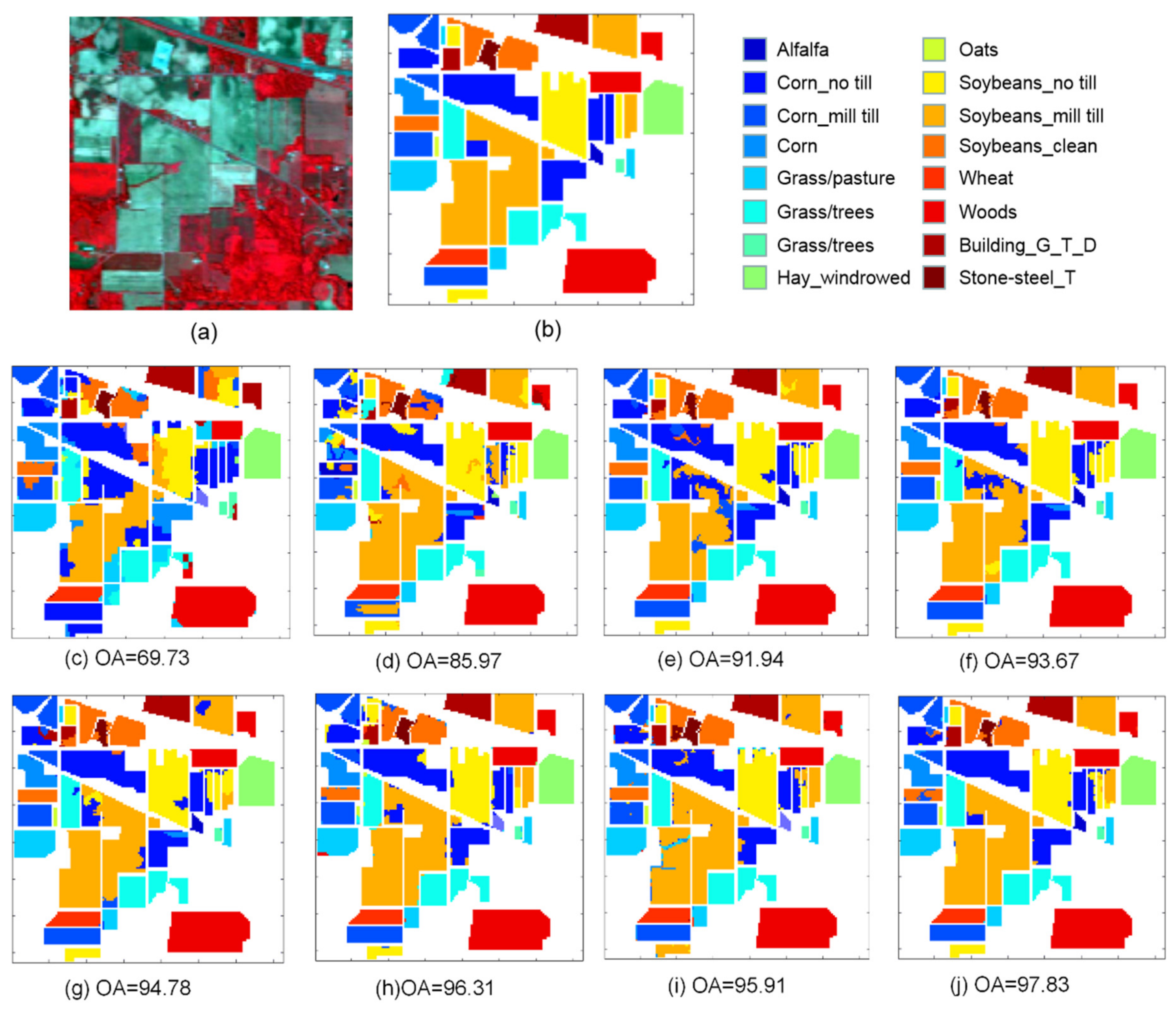
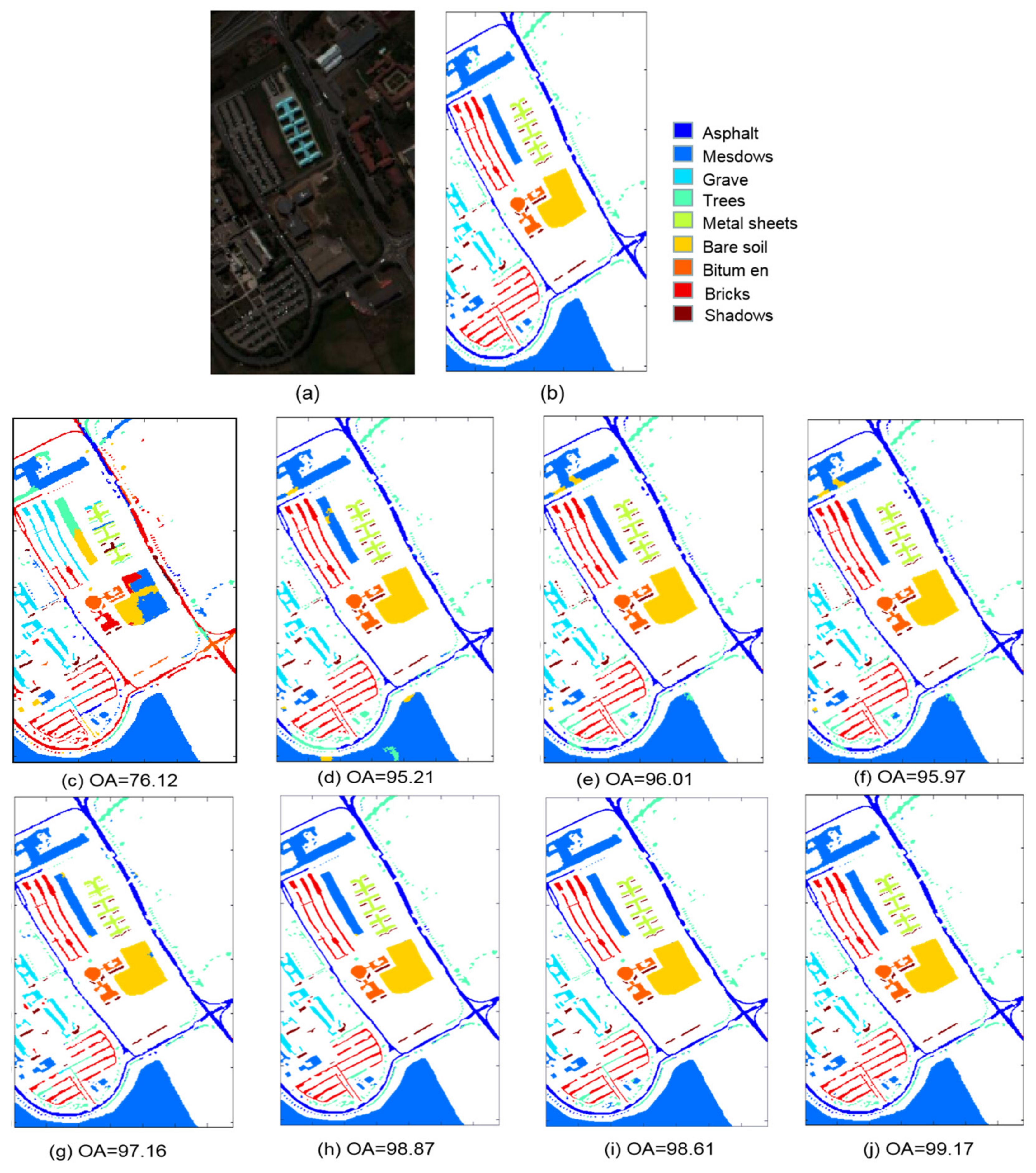
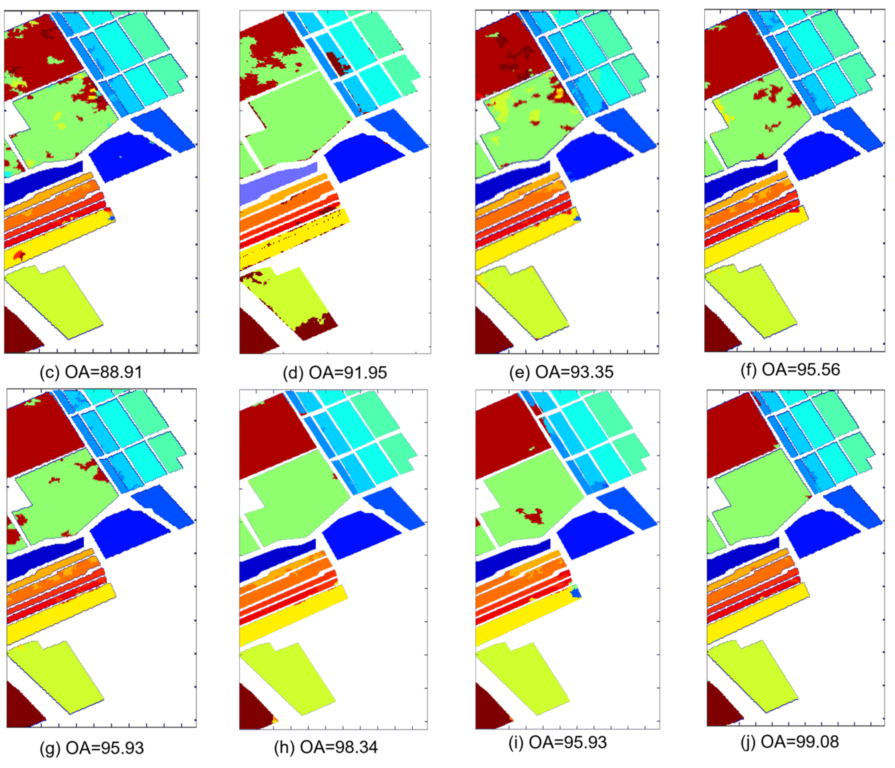
3.3. Classification Results

The classification results of seven competitors and our method on Indian Pines image are tabulated in

Table 2. Classification results (%) of eight methods for Indian Pines image.

	GCN	EPF	IFRF	SCMK	SSC-SL	MDGCN	SPCNN	SSG
1	93.65 ± 0.35	26.28 ± 6.43	94.41 ± 1.86	95.25 ± 0	76.51 ± 3.67	90.23 ± 1.47	96.38 ± 0.92	97.39 ± 1.95
2	51.36 ± 1.83	68.69 ± 5.64	86.14 ± 3.68	90.07 ± 2.54	94.65 ± 2.01	93.37 ± 1.22	91.96 ± 0.41	97.46 ± 0.55
3	50.30 ± 3.02	58.74 ± 2.62	84.67 ± 4.67	92.89 ± 3	92.4 ± 1.71	92.66 ± 4.70	95.80 ± 1.82	97.87 ± 1.49
4	25.41 ± 6.98	40.89 ± 18.71	73.16 ± 6.67	84.51 ± 3.44	71.25 ± 9.75	94.80 ± 5.68	89.61 ± 0.18	98.39 ± 2.16
5	0 ± 0	91.77 ± 2.51	91.18 ± 4.52	93.57 ± 4.20	92.07 ± 3.67	93.34 ± 3.44	89.32 ± 2.16	95.57 ± 1.87
6	97.52 ± 1.42	99.73 ± 2.77	98.44 ± 1.12	98.68 ± 1.15	99.34 ± 0.79	97.89 ± 0.70	99.04 ± 0.29	99.81 ± 0.06
7	98.3 ± 2.34	93.46 ± 8.07	94.62 ± 10.77	96.17 ± 1.35	97.31 ± 4.07	90.77 ± 7.30	95.1 ± 2.28	96.43 ± 0.24
8	97.46 ± 0.37	99.96 ± 0.13	100 ± 0	99.62 ± 0.15	94.58 ± 4.47	99.47 ± 0.56	99.39 ± 0.02	100 ± 0
9	100 ± 0	0 ± 0	100 ± 0	46.62 ± 5.21	82.63 ± 5.22	57.37 ± 30.93	95.06 ± 1.14	100 ± 0
10	73.58 ± 1.73	68.63 ± 4.93	87.56 ± 3.39	91.36 ± 2.56	93.65 ± 1.54	93.26 ± 1.46	92.48 ± 2.17	94.01 ± 0.74
11	78.38 ± 5.82	93.64 ± 2.91	98.03 ± 0.59	95.19 ± 1.9	96.84 ± 0.85	97.50 ± 0.78	81.02 ± 2.41	98.60 ± 0.81
12	56.37 ± 2.27	54.49 ± 13.27	74.46 ± 9.43	91.3 ± 2.2	85.81 ± 4.08	92.43 ± 3.17	97.83 ± 0.02	95.95 ± 1.76
13	99.01 ± 0.09	99.43 ± 0.15	99.07 ± 0.6	97.42 ± 1.23	98.09 ± 2.85	99.23 ± 1.24	99.43 ± 0.02	99.12 ± 0.43
14	99.6 ± 0.08	99.54 ± 0.25	98.75 ± 0.92	99.3 ± 0.56	98.96 ± 0.63	99.78 ± 0.13	96.36 ± 0.17	99.84 ± 0.08
15	76.67 ± 2.40	57.9 ± 12.90	94.97 ± 3.11	92.94 ± 3.76	95.33 ± 3.79	96.39 ± 5.71	100 ± 0	98.86 ± 0.28
16	89.24 ± 2.54	98.98 ± 1.07	98.86 ± 1.17	86.69 ± 6.51	71.14 ± 3.88	95.80 ± 2.98	98.15 ± 0.60	95.70 ± 1.52
OA	67.86 ± 0.59	82.59 ± 1.42	91.94 ± 1.38	94.21 ± 0.54	94.29 ± 0.61	95.83 ± 0.32	95.26 ± 0.53	97.85 ± 0.07
AA	70.79 ± 3.26	72.01 ± 3.17	92.15 ± 3.28	90.76 ± 3.05	90.05 ± 5.6	92.77 ± 2.33	94.89 ± 1.16	97.75 ± 1.80
κ	63 ± 0.02	80 ± 0.16	91 ± 0.43	93 ± 0.06	91 ± 0.01	95 ± 0.01	94 ± 0.01	98 ± 0.08

. The classification accuracy obtained by the five superpixel-level classification methods is better than that of the other three pixel-wise classification algorithms. This may be due to the fact that the spatial spectral information of this image can be more fully explored by using adaptive size and shape of superpixels in the classification. Compared with IFRF, the accuracy of EPF method is relatively low (82.59%), probably because the edge-preserving filtering technique is only used in the classification maps to correct misclassified pixels. The classification accuracy of our method is improved by at least 2% (97.85% vs. 95.83%) contrast to other four superpixel-level competitors, SCMK, SSC-SL, MDGCN and SPCNN. Furthermore, the proposed SSG method outperforms other competitive algorithms in terms of the three evaluation indicators. The visualization of classification results of eight different methods are shown in Figure 3.

For Indian Pines image, there are 145 × 145 (21,025) pixels. Among them, the number of pixels to be classified is 10,249. The classification accuracy 97.83% means that there are about 223 misclassification pixels. Assuming that this image is divided into 1000 superpixels, each one contains approximately 20 pixels. Therefore, at least 21 superpixels are misclassified because of many misclassified small volume superpixels produced after removing the background pixels. This is why the visuals are unsatisfactory.

Table 3. Statistical results (%) of seven competitive algorithms and the proposed method for Pavia University image.

	GCN	EPF	IFRF	SCMK	SSC-SL	MDGCN	SPCNN	SSG
1	62.85 ± 12.37	99.75 ± 0.43	97.54 ± 1.06	95.94 ± 0.82	99.32 ± 0.12	99.24 ± 0.33	99.03 ± 0.06	99.76 ± 0.08
2	58.07 ± 2.23	99.94 ± 0.22	99.85 ± 0.14	95.65 ± 0.29	99.92 ± 0.05	99.73 ± 0.07	99.26 ± 0.03	99.95 ± 0.04
3	46.56 ± 9.28	72.32 ± 5.33	84.08 ± 5.18	93.60 ± 4.87	78.28 ± 0.25	97.25 ± 0.99	99.19 ± 0.04	99.37 ± 0.48
4	53.45 ± 8.45	95.77 ± 0.69	93.04 ± 1.24	95.74 ± 0.83	96.46 ± 0.21	96.22 ± 1.02	98.94 ± 0.16	88.11 ± 0.65
5	88.72 ± 2.51	99.92 ± 0.23	99.83 ± 0.13	94.33 ± 0.15	99.92 ± 0.29	98.56 ± 1.06	100 ± 0	99.73 ± 0.13
6	59.57 ± 6.22	77.25 ± 0.07	99.75 ± 0.03	96.16 ± 1.29	90.24 ± 0.06	99.99 ± 0.03	99.27 ± 0.02	99.90 ± 0.07
7	88.81 ± 2.27	90.50 ± 0.39	97.66 ± 1.32	92.23 ± 5.82	91.53 ± 0.26	97.92 ± 1.98	99.32 ± 0.04	100 ± 0
8	76.06 ± 2.26	98.91 ± 0.85	86.41 ± 2.12	95.2 ± 1.06	98.91 ± 0.15	96.14 ± 1.32	98.45 ± 0.04	98.65 ± 1.51
9	81.34 ± 4.52	96.89 ± 3.37	42.67 ± 2.68	97.59 ± 0.6	97.33 ± 0.28	93.58 ± 2.27	98.26 ± 0.68	99.62 ± 0.55
OA	75.78 ± 2.64	95.14 ± 0.32	95.73 ± 0.32	96.49 ± 0.15	96.47 ± 0.03	98.77 ± 0.13	98.53 ± 0.03	99.12 ± 0.12
AA	77.50 ± 3.57	92.36 ± 1.28	88.98 ± 4.30	95.29 ± 2.86	94.66 ± 0.19	97.63 ± 0.38	99.06 ± 0.28	98.34 ± 3.64
κ	75 ± 0.04	93 ± 0.43	94 ± 0.24	96 ± 0.19	96 ± 0.01	98 ± 0.01	98 ± 0.01	99 ± 0.15

reports the statistical results of eight algorithms on Pavia University scene. With the exception of the GCN method, the classification results of all spatial-spectral methods are satisfactory (greater than 95%) because of the high resolution of the image and the good spatial separation between classes. Both MDGCN, SPCNN and our method have a classification accuracy of more than 98.5%. There is no significant difference in the classification results of these three methods. This shows that the proposed method is comparable to that based on deep learning. Compared with EPF, IFRF, SCMK and SSC-SL methods, the classification accuracy raised by at least 2.6%. Of the eight approaches, the GCN method has the lowest classification accuracy. The reason should be that, on the one hand, this method utilizes only spectral information for pixel-wise classification. On the other hand, the neural network classifier adopted in GCN requires a large number of training samples to achieve satisfactory result. The classification maps of these methods are presented in Figure 4.

Table 4. Classification results (%) of eight spatial-spectral approaches on Salinas.

	GCN	EPF	IFRF	SCMK	SSC-SL	MDGCN	SPCNN	SSG
1	100 ± 0	99.59 ± 1.10	99.80 ± 0.02	100 ± 0	100 ± 0	100 ± 0	100 ± 0	100 ± 0
2	99.78 ± 0.05	99.86 ± 0.16	99.21 ± 0.26	99.78 ± 0	97.84 ± 0.17	99.85 ± 0.16	99.16 ± 0.02	100 ± 0
3	100 ± 0	88.18 ± 3.03	100 ± 0	97.11 ± 0.76	98.38 ± 5.13	99.36 ± 0.93	100 ± 0	100 ± 0
4	92.38 ± 0.25	99.56 ± 0.17	96.27 ± 2.26	95.78 ± 3.33	96.07 ± 6.44	96.12 ± 4.79	99.67 ± 0.04	95.56 ± 2.73
5	98.91 ± 0.16	99.26 ± 0.34	97.79. ± 0.43	94.95 ± 0.21	96.9 ± 0.2	96.94 ± 0.88	99.21 ± 0.07	97.21 ± 1.44
6	99.67 ± 0.21	99.98 ± 0.01	99.28 ± 0.01	99.69 ± 0.18	95.88 ± 0.05	99.93 ± 0.01	99.02 ± 0.12	100 ± 0
7	99.40 ± 0.04	99.75 ± 0.03	99.57 ± 0.21	95.27 ± 0.31	99.85 ± 0.1	99.48 ± 0.70	99.07 ± 0.04	99.80 ± 0.13
8	68.78 ± 0.63	92.49 ± 0.03	74.34 ± 9.24	93.01 ± 2.7	95.53 ± 1.01	99.02 ± 0.82	98.45 ± 0.80	99.52 ± 0.33
9	99.90 ± 0.01	99.5 ± 0.62	99.98 ± 0	96.67 ± 1.85	96.77 ± 0.29	99.99 ± 0.03	99.81 ± 0.01	99.93 ± 0.05
10	91.91 ± 0.43	90.71 ± 1.65	98.94 ± 0.97	96.38 ± 1.24	96.84 ± 1.78	98.89 ± 0.82	98.61 ± 0.07	98.75 ± 0.40
11	99.19 ± 0.03	97.68 ± 1.32	93.87 ± 3.93	94.19 ± 3.39	98.19 ± 0.81	96.40 ± 1.81	100 ± 0	96.27 ± 2.11
12	87.66 ± 0.91	100 ± 0	98.26 ± 2.56	97.34 ± 3.23	100 ± 0	93.32 ± 3.91	93.42 ± 1.03	93.95 ± 1.84
13	98.04 ± 0.28	97.79 ± 0.42	86.24 ± 6.85	97.12 ± 0	96.83 ± 3.11	87.48 ± 13.82	98.44 ± 0.11	98.07 ± 0.19
14	95.21 ± 1.30	93.54 ± 6.21	93.45 ± 1.46	95.46 ± 3.68	92.96 ± 6.41	91.08 ± 3.37	93.22 ± 0.07	95.44 ± 2.38
15	69.01 ± 2.27	59.94 ± 2.47	89.62 ± 9.58	93.5 ± 3.33	95.04 ± 1.73	98.02 ± 1.76	93.69 ± 2.46	99.26 ± 0.33
16	97.22 ± 0.35	97.51 ± 2.96	97.51 ± 0.47	94.64 ± 4.66	94.05 ± 0.34	99.11 ± 2.12	96.71 ± 0.25	97.71 ± 1.97
OA	88.67 ± 0.96	91.55 ± 1.87	92.06 ± 2.07	96.01 ± 0.27	96.83 ± 0.36	98.41 ± 0.35	95.88 ± 0.14	98.97 ± 0.08
AA	88.63 ± 1.03	94.51 ± 2.7	92.59 ± 3.71	96.12 ± 1.80	96.01 ± 1.72	97.19 ± 0.81	98.02 ± 1.36	98.22 ± 1.92
κ	87 ± 0.01	91 ± 0.32	91 ± 0.58	96 ± 0.03	95 ± 0.04	98 ± 0.01	95 ± 0.12	99 ± 0.10

lists the classification results of various algorithms for Salinas image. The classification accuracy of seven methods is greater than 90% in the case of 1% pixels randomly labeled per class. The classification accuracy of EPF and IFRF methods is 91.55% and 92.06%, respectively, which is lower than that of the other five superpixel based methods. It may be due to the use of dimensionality reduction technique in these two methods, resulting in the loss of some information. There was no significant difference in classification results (from 95. 88% to 96.83%) among of SCMK, SSC-SL and SPCNN methods since they all used spatial adaptation technique. Our method is slightly better than the MDGCN method, which reaches 98.97%. In particular, for the two classes easily misclassified, i.e., the 8-th class and the 15-th class, the average accuracy of 99.52% and 99.26% indicates the superior performance of our method locally. As can be seen from Figure 5, our method shows good classification performance in both the global and local regions.

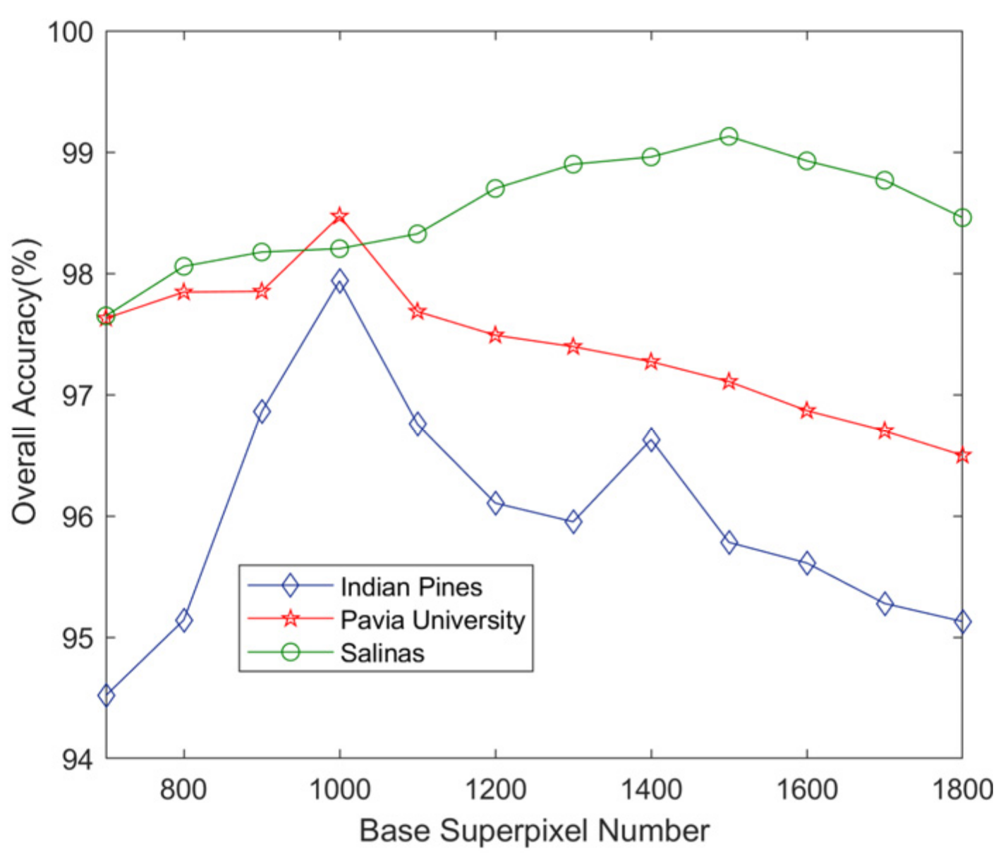
4. Effect of the Number of Superpixels and Different Number of Training Samples

The classification results of our proposed scheme depend on the choice of superpixel number and labeled sample number. As with many existing superpixel-based methods, the optimal parameter value was obtained as an experimental result, not as a pre-specified one. Therefore, the effect of different superpixel number and different number of training samples on the performance of the proposed SSG approach will be analyzed in this section. The OA values recorded in our experiments are the average of ten independent runs.

In our experiments, the test superpixel number was from 700 to 1800. The number of training samples and test samples is the same as that listed in Table 1. In Figure 6, with the increase of the number of superpixels, the change of OA values shows a similar trend on three scenes, that is, rising first and then decreasing. The difference between them is that the superpixel number corresponding to the optimal OA value and the magnitude of the change are different. The reason may be that a small superpixel number usually means that the generated superpixels have large sizes. This increases the risk that the objects belonging to different classes are located in the same superpixel. In addition, although the superpixel with small size has better homogeneity, it weakens the role of spatial information in classification. The experimental results show that when the number of superpixels is equal to 1000 for Indian Pines and Pavia University images and 1500 for Salinas image, our method provides satisfactory classification results on three scenes.

The performance of semi-supervised classification methods generally relies on the number of training samples. Although excellent classification results can be obtained using a large number of training samples, the marking of samples is expensive. Thus, using a small number of labeled samples to obtain satisfactory classification results can often verify the performance of the classifier. The number of superpixels is identical to that determined in the previous part. Figure 7 displays the impact of different numbers of training sample on several classification methods. The number of randomly labeled pixels per class varies from 5 to 30 for these three scenes. It is easy to see that the classification accuracy of all methods gradually improves as the increase of training pixels. Due to lack of spatial information and the use of neural network in classification, the classification results of GCN were unsatisfactory. Compared with other six spectral-spatial classification algorithms, the proposed scheme can always acquire better performances for different numbers of training samples for different images.

Additionally, we further compared the running time of these classification methods. All experiments were implemented using MATLAB 2018a on the computer with TM i7-6700 CPU, 3.40GHz, 16GB memory and NVIDIA GEFORCE RTX 1660 GPU. The running time here includes all the computational times for PCA, ERS, graph construction, label propagation and classification.

Table 5. Running time (seconds) of eight classification methods on three images.

	GCN	EPF	IFRF	SCMK	SSC-SL	MDGCN	SPCNN	OURS
IP	58.72 ± 0.36	13.041 ± 0.36	4.732 ± 0.11	6.23 ± 0.09	15.09 ± 0.56	44.64 ± 0.53	65.83 ± 2.92	1.481 ± 0.01
PU	783.06 ± 2.21	17.564 ± 1.22	12.864 ± 0.56	12.97 ± 0.21	21.33 ± 1.02	154.16 ± 3.86	205.86 ± 3.51	4.267 ± 0.26
SA	73.59 ± 1.64	27.693 ± 0.21	14.122 ± 0.14	14.33 ± 0.21	23.77 ± 0.69	24.53 ± 0.91	51.54 ± 3.73	6.057 ± 0.38

reports the running time (average of ten runs) of these methods on Indian Pines (IP), Pavia University (PU) and Salinas (SA) images with 30 labeled pixels per class. Three deep learning-based classification framework, GCN, MDGCN and SPCNN, are time-consuming since there are massive parameters to be optimized. One can observe from Table 5 that the computation time of our method is less than 10 seconds on three images and much less than that of other competitors. This satisfactory result benefits from the computational efficiency of the ERS algorithm, the abstract representation of superpixels, the computational simplicity of the graph construction and the rapid implementation of solving algebraic equations by CGDM approach. The results in Table 2, Table 3, Table 4 and Table 5 confirm that the proposed method can accurately and quickly realize the classification of hyperspectral data.

5. Discussions

Based on Table 2, Table 3 and Table 4 and earlier studies [10,20,22,27,32,34,35,36,37,38,39,40], although superpixel-based HSI classification methods can achieve better classification results than pixel-based ones, superpixel-based HSI classification methods often suffer from two problems.

One is how to determine the optimal number of superpixels. As shown in Figure 5, different superpixel segmentation scales will result in different classification results. To date, the determination of the optimal number of superpixels still depends on the experimental results [10,20,22,27,32,34,35,36,37,38,39,40]. Although the multiscale-based approach can partially address this problem [18,33], the problem of how to choose segmentation scales still remains. There may be two ways to address this problem: (1) define an indicator to determine superpixel segmentation scale for a given hyperspectral image; (2) eliminate or alleviate the effect of segmentation scale on the classification results by merging superpixels.

The other is how to properly measure the similarity between two superpixels and pixels. Generally, it is difficult to properly define the distance between the two superpixels due to its characteristic of adaptive shape and size. In [32,37,38,39,40], the authors try to use various techniques to address this problem, such as affine hull model [32,38], covariance matrix [40], KNN-based [37,39]. The computation complexity of the distance between two superpixels is at least O $(n_i\times n_j\times B)$ in these studies. In our work, the complexity of calculating the distance between the two superpixels is approximately O $(n_i+n_j)\times B$. As expected, calculating the defined distance is more efficient than existing methods.

In Equation (2), we only consider three commonly used statistical features of superpixels to construct a new sample to approximately represent a superpixel. Perhaps, more factors should be considered in such a representation, for example, the entropy, texture features or variance of superpixels. In addition, it is also important to choose an appropriate metric when calculating the distance between superpixels defined in Equation (3). For example, if the Euclidean distance (ED) in Equation (3) is replaced with spectral angular mapping (SAM) [59], different classification results and running times are obtained, as shown in

Table 6. Classification results and running time (seconds) on three images.

	Indian Pines		Pavia University		Salinas
	SAM	ED	SAM	ED	SAM	ED
OA	94.8 ± 2.01	97.85 ± 0.07	97.97 ± 0.27	99.12 ± 0.12	92.12 ± 4.21	98.97 ± 0.08
AA	93.02 ± 9.58	97.75 ± 1.80	96.36 ± 4.82	98.34 ± 3.64	88.67 ± 8.98	98.22 ± 1.92
κ	94.1 ± 2.28	98 ± 0.08	97.54 ± 0.39	99 ± 0.15	91.26 ± 4.65	99 ± 0.10
Times	1.82 ± 0.50	1.481 ± 0.01	4.75 ± 0.07	4.267 ± 0.26	6.375 ± 0.08	6.057 ± 0.38

. In general, using different metrics may yield different classification results for the same classification algorithm. Thus, it is necessary to choose the appropriate metrics for different data types.

It is also important to select the appropriate metrics when calculating the distance between the superpixels defined in Formula (3).

Additionally, the sparse superpixel graph constructed here is an unweighted graph. Thus, some popular graph partitioning algorithms can be used directly. Theoretically, weighted directed graphs can better represent the close relationship between vertices. However, the intimacy between the two vertices is often asymmetric. In this case, the proposed method cannot work well, and a redesign of new label propagation method is required. Therefore, it is still worth to further explore how to represent hyperspectral data with a weighted directed superpixel graph and study its division.

6. Conclusions

Based on the constructed superpixel graph and discrete potential theory, in this work, we present a superpixel-level semi-supervised HSI classification method. The merits of the proposal are the following: (i) Unlike the existing definition of distance between superpixels, the only use of a vector to approximately represent a superpixel makes it easy and fast to calculate the defined distance between a pair of superpixels. (ii) The classification results of three scenes demonstrate that the strategy of global spectral connection and local spatial connection can better preserve the spectral and spatial relations of the HSI in the constructed superpixel graph. (iii) In the constructed superpixel graph, taking each superpixel as a vertex instead of a pixel actually reduces the hyperspectral data spatially, so that our method can be realized quickly. (iv) The label propagation procedure based on discrete potential theory, the CGDM and approximate solution speeds up the implementation of the scheme again. Experimental and comparative results in this paper, respectively, confirm the validity of the proposed classification scheme and outperform other state-of-the-art methods in terms of classification accuracy and running time.

References

1. He, X.; Chen, Y.; Ghamisi, P. Heterogeneous transfer learning for hyperspectral image classification based on convolutional neural network. IEEE Trans. Geosci. Remote Sens. 2019, 58, 3246–3263. [Google Scholar] [CrossRef]
2. Jiao, L.; Feng, J.; Liu, F.; Sun, T.; Zhang, X. Semisupervised affinity propagation based on normalized trivariable mutual information for hyperspectral band selection. IEEE J. Sel. Top. Appl. Earth Obs. Remote Sens. 2014, 8, 2760–2773. [Google Scholar] [CrossRef]
3. Romaszewski, M.; Glomb, P.; Cholewa, M. Semi-supervised hyperspectral classification from a small number of training samples using a co-training approach. ISPRS J. Photo. Remote Sens. 2016, 121, 60–76. [Google Scholar] [CrossRef]
4. Sellami, A.; Farah, M.; Riadh, I.; Solaiman, F. Hyperspectral imagery classification based on semi-supervised 3-D deep neural network and adaptive band selection. Expert Syst. Appl. 2019, 129, 246–259. [Google Scholar] [CrossRef]
5. Fang, B.; Li, Y.; Zhang, H.; Chan, J. Collaborative learning of lightweight convolutional neural network and deep clustering for hyperspectral image semi-supervised classification with limited training samples. ISPRS J. Photo. Remote Sens. 2020, 161, 164–178. [Google Scholar] [CrossRef]
6. Benediktsson, J.; Palmason, J.; Sveinsson, J. Classification of hyperspectral data from urban areas based on extended morphological profiles. IEEE Trans. Geosci. Remote Sens. 2005, 43, 480–491. [Google Scholar] [CrossRef]
7. Clark, M.; Roberts, D. Species-level differences in hyperspectral metrics among tropical rainforest trees as determined by a tree-based classifier. Remote Sens. 2012, 4, 1820–1855. [Google Scholar] [CrossRef] [Green Version]
8. Kanning, M.; Siegmann, B.; Jarmer, T. Regionalization of uncovered agricultural soils based on organic carbon and soil texture estimations. Remote Sens. 2016, 8, 927. [Google Scholar] [CrossRef] [Green Version]
9. Xie, X.; Li, B. A unified framework of multiple kernels learning for hyperspectral remote sensing big data. J. Inf. Hiding Multim. Signal Process. 2016, 7, 296–303. [Google Scholar]
10. Xie, F.; Gao, Q.; Jin, C.; Zhao, F. Hyperspectral Image Classification Based on Superpixel Pooling Convolutional Neural Network with Transfer Learning. Remote Sens. 2021, 13, 930. [Google Scholar] [CrossRef]
11. Barca, E.; Castrignanò, A.; Ruggieri, S.; Rinaldi, M. A new supervised classifier exploiting spectral-spatial information in the Bayesian framework. Int. J. Appl. Earth Obs. Geo. 2019, 86, 101990. [Google Scholar] [CrossRef]
12. Mukherjee, S.; Prasad, S. A spatial-spectral semisupervised deep learning framework using siamese networks and angular loss. Comput. Vis. Image Underst. 2020, 194, 102943. [Google Scholar] [CrossRef]
13. Kizel, F.; Benediktsson, J. Spatially Enhanced Spectral Unmixing Through Data Fusion of Spectral and Visible Images from Different Sensors. Remote Sens. 2020, 12, 1255. [Google Scholar] [CrossRef] [Green Version]
14. Ghamisi, P.; Mura, M.; Benediktsson, J. A Survey on Spectral-Spatial Classification Techniques Based on Attribute Profiles. IEEE Trans. Geosci. Remote Sens. 2015, 53, 2335–2353. [Google Scholar] [CrossRef]
15. Ghamisi, P.; Benediktsson, J.; Cavallaro, G.; Plaza, A. Automatic Framework for Spectral-Spatial Classification Based on Supervised Feature Extraction and Morphological Attribute Profiles. IEEE J. Sel. Top. Appl. Earth Obs. Remote Sens. 2014, 7, 2147–2160. [Google Scholar] [CrossRef]
16. Camps-Valls, G.; Shervashidze, N.; Borgwardt, K. Spatio-Spectral Remote Sensing Image Classification with Graph Kernels. IEEE Geosci. Remote Sens. Lett. 2010, 7, 741–745. [Google Scholar] [CrossRef]
17. Li, J.; Bioucas-Dias, J.; Plaza, A. Spectral-spatial hyperspectral image segmentation using subspace multinomial logistic regression and Markov random fields. IEEE Trans. Geosci. Remote Sens. 2012, 50, 809–823. [Google Scholar] [CrossRef]
18. Dundar, T.; Ince, T. Sparse Representation-Based Hyperspectral Image Classification Using Multiscale Superpixels and Guided Filter. IEEE Geosci. Remote Sens. Lett. 2019, 16, 246–250. [Google Scholar] [CrossRef]
19. Li, J.; Khodadadzadeh, M.; Plaza, A.; Jia, X.; Bioucas-Dias, J. A discontinuity preserving relaxation scheme for spectral–spatial hyperspectral image classification. IEEE J. Sel. Top. Appl. Earth Obs. 2017, 9, 625–639. [Google Scholar] [CrossRef]
20. Xie, F.; Lei, C.; Yang, J.; Jin, C. An effective classification scheme for hyperspectral image based on superpixel and discontinuity preserving relaxation. Remote Sens. 2019, 11, 1149. [Google Scholar] [CrossRef] [Green Version]
21. Kang, X.; Li, S.; Benediktsson, J. Feature Extraction of Hyperspectral Images with Image Fusion and Recursive Filtering. IEEE Trans. Geosci. Remote Sens. 2014, 52, 3742–3752. [Google Scholar] [CrossRef]
22. Fang, L.; Li, S.; Duan, W.; Ren, J.; Benediktsson, J.A. Classification of Hyperspectral Images by Exploiting Spectral-Spatial Information of Superpixel via Multiple Kernels. IEEE Trans. Geosci. Remote Sens. 2015, 53, 6663–6674. [Google Scholar] [CrossRef] [Green Version]
23. Camps-Valls, G.; Gomez-Chova, L.; Muñoz-Marí, J.; Vila-Francés, J.; Calpe-Maravilla, J. Composite Kernels for Hyperspectral Image Classification. IEEE Trans. Geos. Remote Sens. Lett. 2006, 3, 93–97. [Google Scholar] [CrossRef]
24. Xie, F.; Hu, D.; Li, F.; Yang, J.; Liu, D. Semi-Supervised Classification for Hyperspectral Images Based on Multiple Classifiers and Relaxation Strategy. ISPRS Int. J. Geo-Info. 2018, 7, 284. [Google Scholar] [CrossRef] [Green Version]
25. Tarabalka, Y.; Benediktsson, J.; Chanussot, J.; Tilton, J. Multiple Spectral–Spatial Classification Approach for Hyperspectral Data. IEEE Trans. Geosci. Remote Sens. 2010, 48, 4122. [Google Scholar] [CrossRef]
26. He, N.; Paoletti, M.E.; Haut, J.M.; Fang, L.; Li, S.; Plaza, A.; Plaza, J. Feature Extraction with Multiscale Covariance Maps for Hyperspectral Image Classification. IEEE Trans. Geosci. Remote Sens. 2019, 57, 755–769. [Google Scholar] [CrossRef]
27. Xu, H.; Zhang, H.; He, W.; Zhang, L. Superpixel-based spatial-spectral dimension reduction for hyperspectral imagery classification. Neurocomputing 2019, 360, 138–150. [Google Scholar] [CrossRef]
28. Yang, S.; Hou, J.; Jia, Y.; Mei, S.; Du, Q. Hyperspectral Image Classification via Sparse Representation with Incremental Dictionaries. IEEE Geosci. Remote Sens. Lett. 2020, 17, 1598–1602. [Google Scholar] [CrossRef]
29. Chen, Y.; Nasrabadi, N.M.; Tran, T.D. Hyperspectral Image Classification Using Dictionary-Based Sparse Representation. IEEE Trans. Geosci. Remote Sens. 2011, 49, 3973–3985. [Google Scholar] [CrossRef]
30. Zhang, X.; Li, C.; Zhang, J.; Chen, Q.; Feng, J.; Jiao, L.; Zhou, H. Hyperspectral Unmixing via Low-rank Representation with Space Consistency Constraint and Spectral Library Pruning. Remote Sens. 2018, 10, 339. [Google Scholar] [CrossRef] [Green Version]
31. Kwan, C.; Gribben, D.; Ayhan, B.; Li, J.; Bernabe, S.; Plaza, A. An Accurate Vegetation and Non-Vegetation Differentiation Approach Based on Land Cover Classification. Remote Sens. 2020, 12, 3880. [Google Scholar] [CrossRef]
32. Cao, X.; Lu, H.; Ren, M.; Jiao, L. Non-overlapping classification of hyperspectral imagery with superpixel segmentation. Appl. Soft Comput. J. 2019, 83, 105630. [Google Scholar] [CrossRef]
33. Zhan, T.; Lu, Z.; Wan, M.; Yang, G. Multiscale Superpixel Kernel-Based Low-Rank Representation for Hyperspectral Image Classification. IEEE Geosci. Remote Sens. Lett. 2020, 17, 1642–1646. [Google Scholar] [CrossRef]
34. Jia, S.; Deng, X.; Xu, M.; Zhou, J.; Jia, X. Superpixel-Level Weighted Label Propagation for Hyperspectral Image Classification. IEEE Trans. Geosci. Remote Sens. 2020, 58, 5077–5091. [Google Scholar] [CrossRef]
35. Fang, L.; Zhuo, H.; Li, S. Super-resolution of hyperspectral image via superpixel-based sparse representation. Neurocomputing 2018, 273, 171–177. [Google Scholar] [CrossRef]
36. Li, Y.; Lu, T.; Li, S. Subpixel-Pixel-Superpixel-Based Multiview Active Learning for Hyperspectral Images Classification. IEEE Trans. Geosci. Remote Sens. 2020, 58, 4976–4988. [Google Scholar] [CrossRef]
37. Xie, F.; Lei, C.; Jin, C.; An, N. A novel spectral-spatial classification method for hyperspectral image at superpixel Level. Appl. Sci. 2020, 10, 463. [Google Scholar] [CrossRef] [Green Version]
38. Lu, T.; Li, S.; Fang, L.; Bruzzone, L.; Benediktsson, J.A. Set-to-set distance-based spectral-spatial classification of hyperspectral images. IEEE Trans. Geosci. Remote Sens. 2016, 54, 1–13. [Google Scholar] [CrossRef]
39. Tu, B.; Wang, J.; Kang, X.; Zhang, G.; Ou, X.; Guo, L. KNN-based representation of superpixels for hyperspectral image classification. IEEE J. Sel. Topics Appl. Earth Obs. Remote Sens. 2018, 11, 4032–4047. [Google Scholar] [CrossRef]
40. Sellars, P.; Avilés-Rivero, A.; Chonlieb, C. Superpixel Contracted Graph-Based Learning for Hyperspectral Image Classification. IEEE Trans. Geosci. Remote Sens. 2020, 58, 4180–4193. [Google Scholar] [CrossRef] [Green Version]
41. Chen, P.; Jiao, L.; Liu, F.; Zhao, Z.; Zhao, J. Adaptive sparse graph learning based dimensionality reduction for classification. Appl. Soft Comput. J. 2019, 82, 105459. [Google Scholar] [CrossRef]
42. Xue, Z.; Du, P.; Li, J.; Su, H. Sparse Graph Regularization for Hyperspectral Remote Sensing Image Classification. IEEE Trans. Geosci. Remote Sens. 2017, 55, 2351–2366. [Google Scholar] [CrossRef]
43. Shao, Y.; Sang, N.; Gao, C.; Ma, L. Spatial and class structure regularized sparse representation graph for semi-supervised hyperspectral image classification. Pattern Recognit. 2018, 81, 81–94. [Google Scholar] [CrossRef]
44. Ahmadi, S.; Mehrshad, N.; Razavi, S. Semisupervised graph-based hyperspectral images classification using low-rank representation graph with considering the local structure of data. J. Elect. Imag. 2018, 27, 063002. [Google Scholar] [CrossRef]
45. Chen, M.; Wang, Q.; Li, X. Discriminant Analysis with Graph Learning for Hyperspectral Image Classification. Remote Sens. 2018, 10, 836. [Google Scholar] [CrossRef] [Green Version]
46. Camps-Valls, G.; Marsheva, T.; Zhou, D. Semi-Supervised Graph-Based Hyperspectral Image Classification. IEEE Trans. Geosci. Remote Sens. 2007, 45, 3044–3054. [Google Scholar] [CrossRef]
47. Leng, Q.; Yang, H.; Jiang, J. Label Noise Cleansing with sparse Graph for Hyperspectral image Classification. Remote Sens. 2019, 11, 1116. [Google Scholar] [CrossRef] [Green Version]
48. Kipf, T.N.; Welling, M. Semi-supervised classification with graph convolutional networks. arXiv 2016, arXiv:1609.02907. [Google Scholar]
49. Ding, Y.; Guo, Y.; Chong, Y.; Pan, S.; Feng, J. Global Consistent Graph Convolutional Network of Hyperspectral Image Classification. IEEE Trans. Instrum. Meas. 2021, 70, 1–16. [Google Scholar]
50. Wan, S.; Gong, C.; Zhong, P.; Du, B.; Zhang, L.; Yang, J. Multiscale Dynamic Graph Convolutional Network for Hyperspectral Image Classification. IEEE Trans. Geosci. Remote Sens. 2020, 58, 3162–3177. [Google Scholar] [CrossRef] [Green Version]
51. Cai, Y.; Zhang, Z.; Liu, X.; Cai, Z. Efficient Graph Convolutional Self-Representation for Band Selection of Hyperspectral Image. IEEE J. Sel. Top. Appl. Earth Obs. Remote Sens. 2020, 13, 4869–4880. [Google Scholar] [CrossRef]
52. Grady, L. Random walks for image segmentation. IEEE Trans. Pattern Anal. Mach. Intell. 2006, 28, 1768–1783. [Google Scholar] [CrossRef] [Green Version]
53. Wang, F.; Zhang, C. Semisupervised learning based on generalized point charge models. IEEE Trans. Neural Netw. 2008, 19, 1307–1311. [Google Scholar] [CrossRef]
54. Liu, D.; Liu, X.; Wang, W.; Bai, H. Semi-supervised community detection based on discrete potential theory. Physica. A 2014, 416, 173–182. [Google Scholar] [CrossRef]
55. Zhang, Q.; Lü, L.; Wang, W.; Zhou, T. Potential theory for directed networks. PLoS ONE 2013, 8, e55437. [Google Scholar] [CrossRef] [PubMed] [Green Version]
56. Liu, E.; Tuzel, O.; Ramalingam, S.; Chellappa, R. Entropy rate superpixel segmentation. In Proceedings of the CVPR2011, Providence, RI, USA, 20–25 June 2011; pp. 2097–2104. [Google Scholar]
57. Golub, G.; Van Loan, C. Matrix Computations; JHU Press: Baltimore, MD, USA, 2012. [Google Scholar]
58. Kang, X.; Li, S.; Benediktsson, J. Spectral-spatial hyperspectral image classification with edge-preserving filtering. IEEE Trans. Geosci. Remote Sens. 2014, 52, 2666–2677. [Google Scholar] [CrossRef]
59. Tumelien, E.; Visockien, J.; Malien, V. The Influence of Seasonality on the Multi-Spectral Image Segmentation for Identification of Abandoned Land. Sustainability 2021, 13, 6941. [Google Scholar] [CrossRef]
Figure 1. The flowchart of the proposed method. PCA: principal component analysis; ERS: entropy rate superpixel segmentation; CGDM: conjugate gradient descent method.
Remotesensing 13 03592 g001
Figure 2. A graph and two generated electrostatic fields. (a) A graph with nine vertices. (b,c) The electrostatic fields generated by known potentials, respectively. Red digits represent the potential assigned to the labeled vertices, and the other numbers are the potentials calculated by the CGDM.
Remotesensing 13 03592 g002
Figure 3. Indian Pines image. (a) The false-color composite image. (b) Ground-truth. The classification maps of (c) GCN, (d) EPF, (e) IFRF, (f) SCMK, (g) SSL-SL, (h) MDGCN, (i) SPCNN and (j) SSG.
Remotesensing 13 03592 g003
Figure 4. Pavia University image. (a) The false-color composite image. (b) Ground-truth. The classification maps of (c) GCN, (d) EPF, (e) IFRF, (f) SCMK, (g) SSL-SL, (h) MDGCN, (i) SPCNN and (j) SSG.
Remotesensing 13 03592 g004
Figure 5. Salinas image. (a) The false-color composite image. (b) Reference image. The classification maps of (c) GCN, (d) EPF, (e) IFRF, (f) SCMK, (g) SSL-SL, (h) MDGCN, (i) SPCNN and (j) SSG.
Remotesensing 13 03592 g005aRemotesensing 13 03592 g005b
Figure 6. Variation of classification results with different superpixel numbers on three scenes.
Remotesensing 13 03592 g006
Figure 7. Change of classification accuracy on three images with the increase of the number of labeled pixels. (a) Indian Pines. (b) Pavia University. (c) Salinas.
Remotesensing 13 03592 g007