Article

Advancing Cave Detection Using Terrain Analysis and Thermal Imagery

1
Department of Biological Sciences and Center for Adaptable Western Landscapes, Northern Arizona University, Flagstaff, AZ 86011, USA
2
Jenness Enterprises, GIS Analysis & Application Design, Flagstaff, AZ 86004, USA
3
School of Forestry, Northern Arizona University, Flagstaff, AZ 86011, USA
4
Department of Mathematics and Statistics, Northern Arizona University, Flagstaff, AZ 86011, USA
5
U. S. Geological Survey, Astrogeology Science Center, Flagstaff, AZ 86001, USA
6
NASA Goddard Space Flight Center, Instrument Systems and Technology Division, Greenbelt, MD 20771, USA
7
Carl Sagan Center, The SETI Institute, Mountain View, CA 94043, USA
*
Author to whom correspondence should be addressed.
Remote Sens. 2021, 13(18), 3578; https://doi.org/10.3390/rs13183578
Submission received: 17 July 2021 / Revised: 3 September 2021 / Accepted: 5 September 2021 / Published: 8 September 2021

Abstract

:
Since the initial experiments nearly 50 years ago, techniques for detecting caves using airborne and spacecraft acquired thermal imagery have improved markedly. These advances are largely due to a combination of higher instrument sensitivity, modern computing systems, and processor-intensive analytical techniques. Through applying these advancements, our goals were to: (1) Determine the efficacy of methods designed for terrain analysis and applied to thermal imagery; (2) evaluate the usefulness of predawn and midday imagery for detecting caves; and (3) ascertain which imagery type (predawn, midday, or the difference between those two times) was most informative. Using forward stepwise logistic (FSL) and Least Absolute Shrinkage and Selection Operator (LASSO) regression analyses for model selection, and a thermal imagery dataset acquired from the Mojave Desert, California, we examined the efficacy of three well-known terrain descriptors (i.e., slope, topographic position index (TPI), and curvature) on thermal imagery for cave detection. We also included the actual, untransformed thermal DN values (hereafter “unenhanced thermal”) as a fourth dataset. Thereafter, we compared the thermal signatures of known cave entrances to all non-cave surface locations. We determined these terrain-based analytical methods, which described the “shape” of the thermal landscape, hold significant promise for cave detection. All imagery types produced similar results. Down-selected covariates per imagery type, based upon the FSL models, were: Predawn— slope, TPI, curvature at 0 m from cave entrance, as well as slope at 1 m from cave entrance; midday— slope, TPI, and unenhanced thermal at 0 m from cave entrance; and difference— TPI and slope at 0 m from cave entrance, as well as unenhanced thermal and TPI at 3.5 m from cave entrance. We provide recommendations for future research directions in terrestrial and planetary cave detection using thermal imagery.

Graphical Abstract

1. Introduction

Reliable detection of caves is required for both terrestrial and planetary speleological research. Improved cave detection on Earth will provide conservation biologists and resource managers with a tool to efficiently identify and prioritize caves for conservation and management [1]. In North America, cave-roosting bats are in decline due to the westward advance of white-nose syndrome. This epizootic disease has resulted in the loss of millions of bats [2] in 33 states and five Canadian provinces [3,4], and is affecting at least 11 cave-roosting hibernating bat species [5]. At a global scale, we simply do not know where most cave-roosting bat species occur—further challenging effective conservation and management efforts.
Caves also represent important habitats for cave-restricted animals. These systems often support troglomorphic (subterranean-adapted) species with narrow geographic ranges (i.e., occurring within a single cave or watershed [6,7,8,9,10,11,12,13,14,15]) and are often represented by small populations [16,17]. Cave entrances have also been identified as important habitats for relict arthropod species from the last glaciation [18,19,20,21,22] and extensive surface disturbance [23,24,25]. While some areas have been identified as hotspots for endemism and diversity [7,26], cave communities in most regions globally remain largely unknown. The use of remote sensing techniques will improve our ability to reliably locate caves; these features can then be prioritized for biological inventories and subsequently managed in accordance with their conservation importance.
From a planetary perspective, detecting caves elsewhere in the solar system will factor prominently into how caves are targeted for future robotic exploration in the search for life [27,28,29,30,31]. Advanced detection capabilities will also enable us to prioritize caves for human habitation on the Moon and Mars [29,32,33,34], and searching for evidence of life on Mars [29,34]. To date, over 1000 Martian [35,36] and more than 200 lunar cave-like features [37,38,39,40] have been confirmed. Additionally, vents and fissures associated with water ice plumes have been identified on several icy moons including Enceladus [41,42], Io [43], Europa [44], and Triton [45]. In total, 2667 subterranean access points (SAP) have been identified across the solar system [31,46]. Additional SAPs and cave-bearing terrains on other planetary bodies including Mercury, Pluto, Titan, and several dwarf planets and comets will require further examination and scrutiny [31,46].
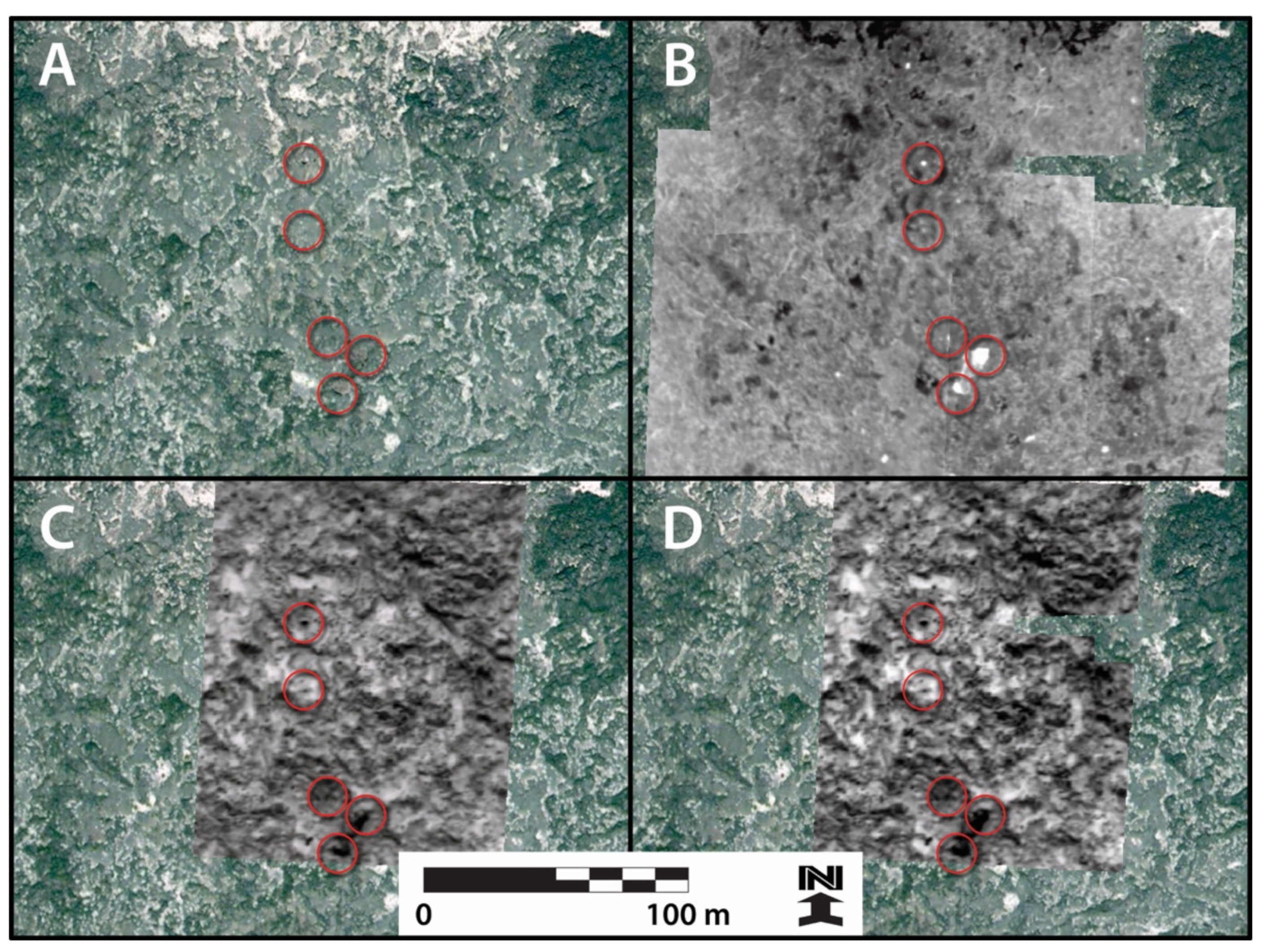
Cave entrances typically appear as warm features in thermal imagery acquired at night and cool features in midday imagery (e.g., [1,36,47,48]) because cave entrances are generally characterized by smaller diurnal temperature changes than the surrounding surface rock. Deep interior cave temperatures are typically stable (e.g., [49,50]) due to diurnal surface temperatures, which are dampened via thermal conduction of the geologic substrate [51,52]. As this occurs, the diurnal temperature variations of cave entrances may also be diminished. The resultant diurnal thermal profile may thus be similar to material with high thermal inertia (e.g., exposed bedrock; [53]).
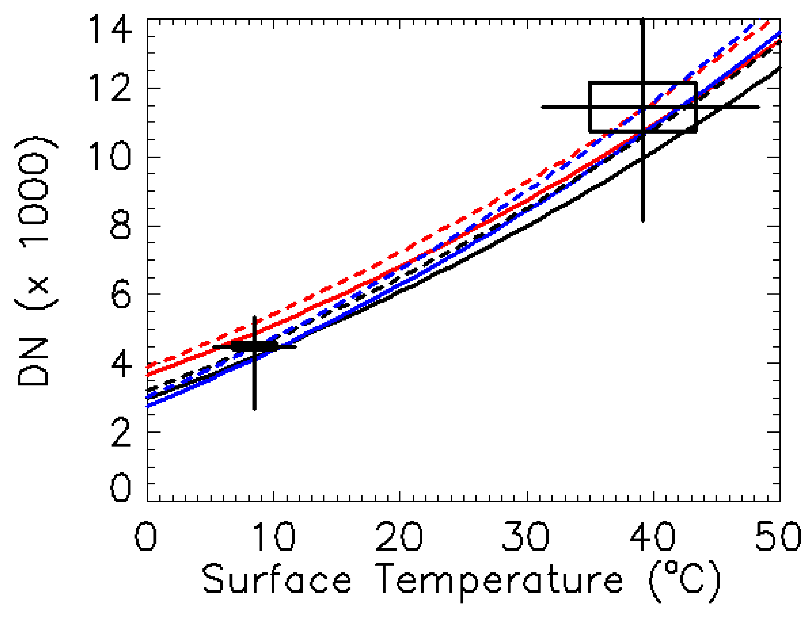
Thermal inertia, a measure of how much an object resists temperature changes and is inherent in all surfaces, is defined as I = k ρ c , where k is thermal conductivity, ρ is density, and c is heat capacity (e.g., [54,55]). Rock surfaces often have higher thermal inertia and therefore exhibit smaller changes in temperature over a diurnal cycle, whereas dust is a common example of a low thermal inertia material.
Rinker [56] was the first to attempt cave detection using thermal instrumentation. He found that caves would be detectable under certain conditions and cautioned that false positives would prove daunting when attempting to identify caves with thermal imagery. This hypothesis went untested for over 30 years. Over the last decade, researchers have re-examined cave detection in the thermal infrared and have made significant advances (e.g., [1,47,57,58,59,60]).
Contemporary work involved collecting and analyzing ground-based temperature measurements and thermal imagery [1,47,57,58,59]. The leap in our ability to detect caves was largely attributed to higher instrument sensitivity, modern computing systems that make processor-intensive analytical techniques possible, and the availability of high accuracy and affordable ground-based meteorological instruments. Analyzing ground-based data from caves in the Atacama Desert of northern Chile, Wynne et al. [1], estimated optimal detection times and demonstrated the utility of ground-based temperature measurements for identifying imagery acquisition times for aircraft-borne missions. Wynne et al. [57] later improved our understanding of cave thermal behavior, proposing three endmembers of cave thermal behavior: Classic, pseudo-classic and ice cave.
Researchers conducted a series of experiments using several generations of QWIP (Quantum Well Infrared Photodetector) thermal instruments [47,61], finding a clear separation between cave, tunnel cave (i.e., a subterranean feature with entrances on either end, typically with frequent air flow), and random non-cave locations on the surface in thermal images captured at 10 min intervals over a 24 h period. Their results suggested how larger caves may be distinguishable from shallow alcoves and tunnel features. Using a similar dataset of thermal imagery, Titus et al. [59] further examined multiple thermal images containing cave entrances over a 24 h period; they reported the detectability of caves was optimal when multiple thermal images were acquired at either the warmest (midday) or coolest times of day (predawn).
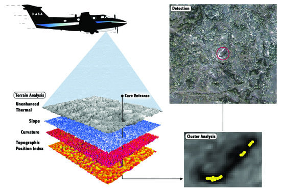
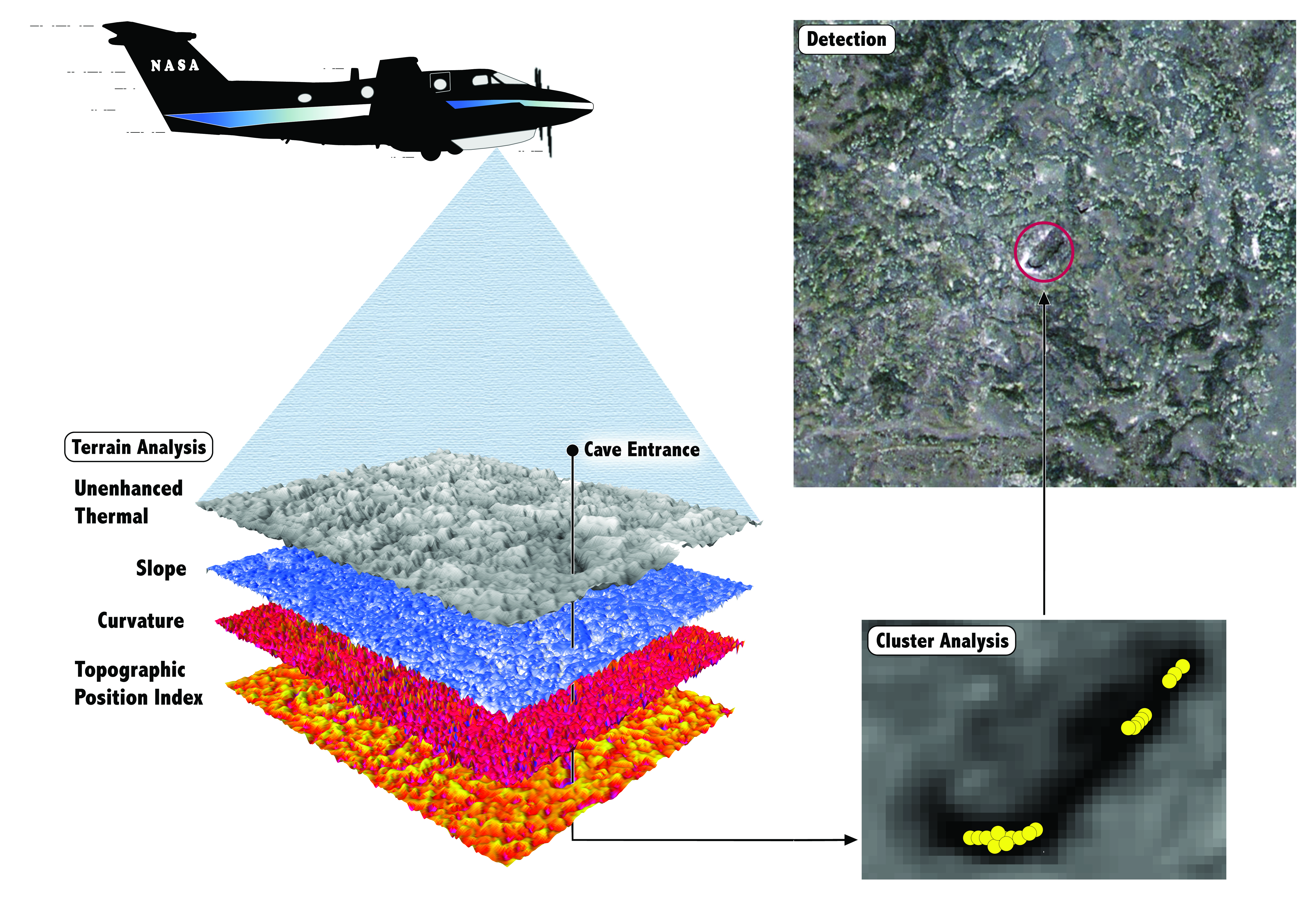
In this paper, we applied advanced image processing techniques to multiple time-of-day thermal imagery to reduce the frequency of false positives. Specifically, we: (1) Determined the efficacy of methods developed for investigating topographic surfaces for thermal imagery analysis; (2) evaluated the usefulness of predawn and midday imagery for detecting caves; and (3) ascertained whether thermal characteristics captured at one time of day (predawn or midday), or the difference in thermal value between those two times, was more informative than another. Specifically, we compared the thermal signatures of cave entrances to all non-cave surface locations using a multivariate framework involving terrain analysis methodology applied to the thermal surface (i.e., topographic position index, slope, and curvature of thermal values) and unenhanced thermal values derived from thermal imagery.

2. Material and methods

2.1. Study Area and Field Data

Pisgah Lava Field (34°44′47″N, 116°22′30″W) is located about 175 miles northeast of Los Angeles, California (Figure 1) and administered by Bureau of Land Management, Barstow Field Office. Situated within the eastern Mojave Desert, this lava field is approximately 21,000 years old [62]. Consisting of numerous thin flows covering approximately 51 km2 and extending from the vent ~18 km to the west and 8 km to the southeast, this lava field is primarily pāhoehoe lava mosaicked by pockets of ʻaʻā lava. This large, sparsely vegetated lava field contains over 300 known lava tube caves [63]. Our focal area within the Pisgah Lava Field was 172 ha in size, with elevations ranging from 680 m to 772 m x ¯ = 702   m , s d = 15.3 . Two missions were flown over Pisgah to acquire thermal imagery—the first occurred from 1222 to 1457 h on 11 April 2011 with the second from 0426 to 0649 h local time on 13 April 2011. These times were selected to minimize temperature changes across the target area. We aimed to acquire predawn data prior to sunrise, while the midday collection was centered around the time of peak temperature (e.g., [64,65]).

2.2. Dataset

2.2.1. Sensor Description, Linear Response, and Pixel Resolution

Thermal imagery was captured using a quantum well infrared photodetector (QWIP) thermal imaging camera, designed by NASA Goddard Space Flight Center in collaboration with QmagiQ, LLC of Nashua, New Hampshire. This experimental instrument was a precursor to the thermal infrared sensor onboard the Landsat 8 spacecraft [66]. Through this work, we collected field performance data to aid in maturing this technology to NASA technology readiness level 5 [67]. The QWIP thermal sensor responds to far infrared radiation from 7.5 to 9.1 μm spectral band with a peak response of 8.7 μm [68]. The detector array was cooled with a miniature Stirling cycle cryocooler to 67K (−206 °C) with a standard 50 mm IR lens and had an instantaneous field of view of 8.8° × 11°. Integration time was 0.0167 s. The camera was preset to capture two 16-bit images/second (2 frames per second). Each image is in a 320 × 256 pixel format where each pixel is a 30 μm square. While the imagery was not radiometrically calibrated, the instrument had the ability to resolve signals from objects where temperature variations were less than 0.02 °C [68]. Additionally, the imagery for both predawn and midday were captured within a ~40 h window, the aircraft power source did not fluctuate, and the instrument was housed within a pressurized aircraft. The camera was stable over time—if the camera was at the same temperature looking at the same object at a given temperature, it would produce the same number of counts (DNs) to within <1% [68].
Titus et al. [69], using the same QWIP instrument, acquired two diurnal sets of oblique thermal images overlooking the Pisgah Lava Field from the approximate mid-elevation point on the Pisgah cinder cone in late March of 2010. In situ temperature data of both the surface and the near surface (~1 m AGL) atmosphere were acquired. They determined the precision of the brightness temperature (no correction for atmosphere or surface emissivity) was accurate to less than 1 °C. Based on the in situ calibration which included atmospheric correction, they reported the surface temperature estimates were accurate to ~3.7 °C at 20 °C. Inadequate characterization of the atmosphere, where the air temperature and humidity data were used, may not accurately represent the conditions along the entire line-of-sight from camera to surface. This was likely the cause for the larger uncertainty in accuracy under field conditions, when compared to laboratory testing results. Refer to Appendix A and Titus et al. [69] for more details.
Average aircraft height above ground level was 808 m for the predawn flight, and 825 m for the midday flight (which was similar to the distance (670 m) between instrument and target for the Titus et al. [69] study). We acquired ~0.5 m resolution data at nadir. A total of 3675 and 4445 images were collected during the predawn and midday flights, respectively. Capture rate was at one and two second intervals for the predawn and midday flights, respectively. Predawn target ground speed varied from 56 m/s when flying in a westerly direction, to 69 m/s easterly. Midday ground speed averaged 63 m/s with little variation between easterly and westerly directions.
No atmospheric corrections were applied. Atmospheric temperature and opacity were not available. However, the analytical techniques employed in this study should be relatively insensitive to the effects of thermal remission and atmospheric absorption. During midday, the observed radiance would decrease as the atmosphere is typically cooler than the observed surface, but the spatial indices would vary little as the atmosphere affect (offset) would be nearly uniform. Atmosphere would likely have even less of an effect for predawn temperatures as surface and atmosphere temperatures would be more similar. Data acquired one year prior using the same QWIP instrument supported this conclusion [69].

2.2.2. Georectification and Processing

We assigned approximate geospatial positions to all imagery using custom Visual Basic for Applications (VBA) functions in ArcGIS (refer to [70]). VBA functions roughly georeferenced, scaled, and oriented each image in its approximate geospatial location using a digital elevation model downloaded from the USGS 3D Elevation Program [71] and aircraft GPS data including time, altitude, and coordinate data. Using both ESRI World Imagery [72] and National Agriculture Imagery Program [73] imagery (1 m resolution) as base reference layers, we manually georeferenced a subset of 49 predawn and 60 midday images that were preselected based on their overlap with known cave locations (refer to Section 2.2.4). All procedures were executed using the Georeferencing Tool in ArcGIS 10.3 [74]. Georeferencing involved identifying reference points apparent on both the reference layer and the thermal images, and then mathematically warping the thermal images to match the base reference layer using a polynomial warping function (in most cases, an affine transformation) that minimized the root mean square error. We used bilinear interpolation to resample the warped image, and then selected a resample resolution that most closely approximated the original resolution. Because we had nadir-viewing imagery, and the elevation range in image footprints (roughly 126 m × 156 m) did not exceed 16.5 m x ¯ = 6.7   m , we determined topographic terrain would not be a major impediment to the georectification process.
We used three datasets for our analysis: Predawn, midday, and difference imagery (Figure 2). For the difference imagery, we reasoned the change between predawn DN values and midday DN values would be relatively low at cave entrances because entrance temperatures fluctuate less compared to the surrounding surface landscape. Thus, the lower pixel values associated with cave entrances would produce a distinguishable signature on the landscape. We mosaicked the best predawn images into a single composite image and repeated this process for midday images. Pixel values in overlapping areas were calculated as the pixel values of the last individual image in the mosaic list. We defined the best images as those with the least amount of geometric distortion required to georeference the image to the landscape. We then generated the difference imagery layer by subtracting the digital number (DN) values of all pixels within the predawn images from the overlapping corresponding DN pixel values in the midday images.

2.2.3. Thermal Transformations Based on Terrain Analysis

The fields of image analysis and object recognition have progressed steadily since the invention of photography and exploded with the advent of computer technology. Software can now, quickly and with high accuracy, recognize and identify obscure and subtle phenomena, such as individual human beings based on facial features or distinguish building footprints from roads or the general landscape. Often the most powerful and interesting methods depend on a specific characteristic of the data being measured. For example, Facebook’s facial recognition software assumes an object in the image has eyes, a nose and a mouth [75]. Similarly, Microsoft’s building footprint algorithm takes advantage of common characteristics of buildings, such as edges and edge angles [76].
As our goal was to identify thermal characteristics that distinguish caves from the general landscape, we identified methods that took advantage of the unique thermal characteristics of caves. Because temperatures at cave entrances tend to be more stable than that of the general landscape, we focused on methods that would specifically measure this thermal characteristic. Additionally, we applied methods that would capture the change in thermal radiance with increasing distance from the cave entrance.
Methods developed for terrain analysis, which measured the rate of change of elevation, were applied to thermal imagery to assess the efficacy of these methods in identifying cave locations. Similar to digital elevation models, thermal imagery depicts temperatures of warm and cool areas appearing as high and low values, and thus presented an opportunity to analyze the thermal “shape” of the landscape. In this case, we treated the thermal surface as a 3D object with peaks, valleys, slopes, and curves. We hypothesized that cave entrances would be distinct features within the 3D thermal surface. To test this idea, we examined the predawn, midday, and difference thermal imagery datasets using the following topographic indices: (1) Topographic position index (TPI), (2) slope (but for thermal imagery should be considered a “thermal gradient”), and (3) curvature. For the predawn, midday, and difference datasets, we also included the actual, untransformed thermal DN values (hereafter “unenhanced thermal”). Figure 3 are histograms for the different imagery datasets for the three topographic indices and the unenhanced thermal.
TPI is the relative value of a specific pixel compared to the mean thermal value of a neighborhood of pixels [77,78], and provides a method for identifying the relatively low and high regions (i.e., local minimum and maximum values) in the thermal surface. In general, TPI serves to identify local valleys and peaks in the thermal surface; valleys represent negative values while peaks are positive values. When applied to our thermal surface, TPI identifies low or high thermal values (relative to their neighbors) and consequently identifies regions that represent a distinct local anomaly. We calculated TPI by first calculating the mean thermal value in a 5 m-radius circular neighborhood around each cell, and then subtracting that neighborhood value from the original cell value. A positive value indicates the area is higher (or warmer, on a thermal surface) than the pixels in the neighborhood. Our ArcGIS model for this technique is provided in [70].
For both slope [79,80] and curvature [81], we used standard ArcGIS algorithms. Given a 3 × 3 neighborhood, with cell values identified as Z1 … Z9, and Z5 being the central cell, and with L = cell edge length, slope is the standard first derivative (the rate of change of thermal values; Equation (1) in the direction of the greatest rate of change.
Slope   in   Degrees = arctan G 2 + H 2 180 π where : G = Z 3 + 2 Z 6 + Z 9 Z 1 + 2 Z 4 + Z 7 8 L H = Z 1 + 2 Z 2 + Z 3 Z 7 + 2 Z 8 + Z 9 8 L
Curvature, in this case, is a measure of overall convexity or concavity of the thermal surface, calculated using the standard “curvature” output in ArcGIS. Conceptually, this is tantamount to the second derivative (the rate of change of slope; Equation (2) but is not defined as the curvature at a point on a line.
C u r v a t u r e = 2 Z 4 + Z 6 2 Z 5 L 2 + Z 2 + Z 8 2 Z 5 L 2 * 100
To avoid highly skewed slope and curvature distributions, we rescaled thermal DN values by dividing by 100 prior to calculating the slope and curvature values. This procedure resulted in more symmetric distributions, which improved our ability to detect patterns along the full range of observed values [82].

2.2.4. Study Sites and Pixel Averaging

Our study sites include several documented caves, which were located and mapped by the Southern California Grotto, National Speleological Society. These included 64 caves (within the midday imagery), 89 caves (predawn imagery), and 37 caves (difference imagery). All caves included in this study had entrances larger than the pixel resolution of the imagery. Given in-flight variations in the pitch, yaw, and roll of the aircraft, we did not acquire seamless and complete coverage of our study area; thus, we did not capture imagery for all known cave locations.
The study caves represent lava tubes of varying lengths and varying numbers of entrances. These include shallow through caves (or tunnels), shelter-like features extending ~10 m to caves tens of meters in length with multiple collapse pit entrances. Given the exploratory nature of this study, we did not attempt to differentiate between shallow caves and caves with a deep zone environment (refer to [49,50]). Thus, we considered all features, regardless of size that permitted access to the subterranean realm, as caves. We also extracted pixel values for all locations on the landscape, which were identified as not being caves. In cases where we had multiple images that included a cave entrance, we used the image that was georeferenced with the least amount of geometric distortion.
We developed TPI, slope, curvature, and unenhanced thermal imagery values for all known cave and non-cave surface locations for each imagery dataset. Because thermal signal strength of cave entrances may be described as a gradation of thermal influence strongest near the center of the cave entrance and diminishing toward the outer edges of the entrance, we attempted to capture this slope using bilinear interpolation [83]. Starting at the center of the cave entrance (0 m) and increasing by 0.5 m concentric intervals, we extracted pixel values from 0 to 3.5 m (Figure 4) and calculated the average for each distance interval. For each interval, we sampled multiple points evenly distributed in a circular pattern, separated by approximately the cell size (roughly 0.5 m). We then took the mean of all values at each distance range to determine the variable value at that distance from the cave. Thus, for each cave entrance location and landscape point, we had 32 covariates ([the four terrain analysis variables] × [average of pixel values at 0.5 m intervals]). For selecting non-cave surface locations, we used the following criteria: (i) Pixels ≥ 10 m from known cave entrances as these areas were most likely to represent non-cave thermal characteristics; (ii) only cave to non-cave locations on the same image were compared to minimize the effects of image-to-image variation; and (iii) only pixel locations that were far enough from the edge of the image to be completely sampled were included in the analysis. Through applying these criteria, we standardized our approach to sampling and analyzing non-cave pixels.

2.3. Analysis

We used 32 terrain covariates (i.e., curvature, slope, TPI, and unenhanced thermal values at the eight distance intervals from the cave entrance or non-cave surface location), which were repeated for each imagery dataset—predawn, midday, and difference. Pearson’s Correlation coefficients (ρ) revealed that most covariates were substantially correlated and therefore interpretation of standard covariate selection methods would be challenging [84]. Therefore, our analysis focused on model prediction accuracy rather than covariate selection. Furthermore, traditional p-values or delta AIC (Akaike Information Criterion) values for each covariate was not appropriate [84]. To avoid over-fitting the models, we applied a machine-learning approach involving feature selection [85]. Our results are presented below.
To select covariates to use, we performed a feature filter procedure [86] whereby we repeatedly and randomly sampled 4000 non-cave surface locations along with all known cave locations (including nine to 21 confirmed caves across the three imagery datasets). For each resulting ‘filtered’ sample, we performed a classic model selection routine ultimately restricting ourselves to using only covariates that were selected in more than 50% of the model runs. We considered two classic model selection routines: Forward stepwise logistic regression (FSL [87]) using AIC [88] and Least Absolute Shrinkage and Selection Operator (LASSO) on logistic regression utilizing 10-fold cross validation [85] for covariate selection. Both are common model selection methods for remote sensing applications (e.g., [89,90,91,92,93,94,95]). We aggregated the filtered sample results by including only covariates that were selected in more than 50% of the filtered samples. As a result of the two model selection techniques (which were designated FSL and LASSO), this became our competing models’ framework.
As most classification models are binary (i.e., positive/negative, success/failure, true/false, etc.), there is some tuning parameter (c) which controls how strong the evidence must be before we predict a positive state (i.e., a cave and not the landscape). High classification thresholds result in higher misclassifications of caves as landscape (false negatives), while lower values result in higher misclassification of landscape pixels as caves (false positives). Fine tuning the model to lower the false negative rate inevitably raises the false positive rate. Therefore, when creating binary classification models for prediction, the threshold parameter tuning process must include a step to balance the false positive and false negative rates. Receiver operator characteristic (ROC) curves vary the model threshold to predict a positive state (c) and then plot the model’s false positive rate verses the true positive rate over a range of thresholds. These ROC curves graphically depict classification curves (i.e., correct classification vs. misclassification) for known cave and non-cave landscape pixels. The quality of the classifier can be assessed from these curves by examining the area under the curve. A value of 1 represents a perfect classifier, while a value of 0.5 (a 1-to-1 line on the ROC curve) indicates the classifier is no better than a random guess.
Because our models were developed at the pixel-level employing the grid pixel extraction technique and not based on the total number of pixels that represent actual cave entrances, we grouped pixels into spatial clusters (code available in GitHub repository https://github.com/JeffJenness/Cave-Detection-Cluster-Analysis, accessed on 2 July 2021) to examine pixel aggregations of both known caves and regions of the non-cave landscape that the model identified as being cave-like. Pixel p ^ values ranged from 0 (lowest similarity to known caves) to 1 (highest similarity to known caves). Thus, we arbitrarily selected the highest 0.01% of pixel p ^ values, which were identified as being similar to cave entrances for each imagery type. Pixels were then grouped into clusters that were within a 2 m threshold distance of at least one other pixel within that cluster. Clusters were classified as being related to a known cave entrance if at least one pixel within the cluster was within the threshold distance of a known entrance. If clusters did not occur near known cave entrances, these aggregations represented either potential new caves or false positives.
We chose to use a custom clustering technique rather than other standard techniques (such as the ArcGIS “Hot Spot” analysis) for this step of the analysis. Specifically, we were most interested in grouping adjacent or highly proximal pixels that likely represented multiple observations of a single cave entrance. Our customized approach enabled us to set a distance threshold for grouping similar pixels.

3. Results

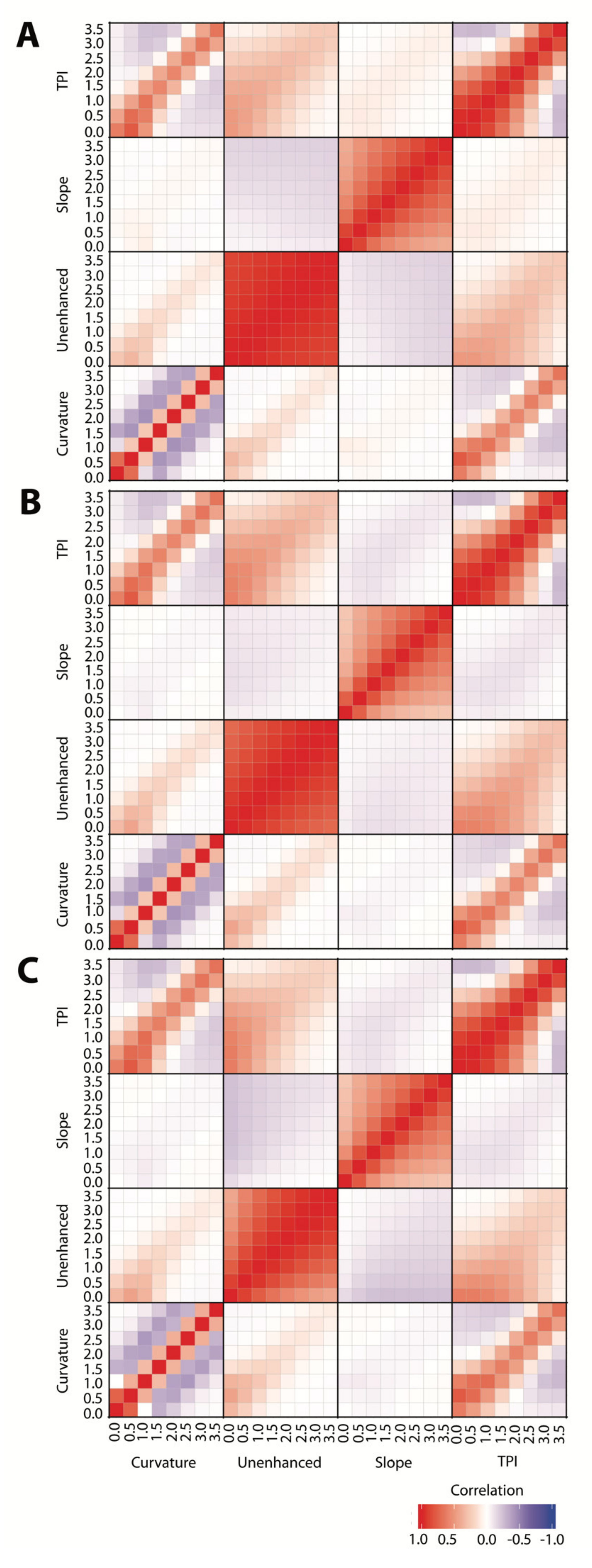
Pearson’s correlations revealed high correlations across most paired comparisons of covariates. Variables were correlated within and between different variables and distances from cave entrances (e.g., slope 1.0 m vs. 2.0 m, as well as slope 0 m vs. TPI 0 m; Figure 5), as well as spatially (e.g., two surface locations within 3.5 m were highly spatially autocorrelated).
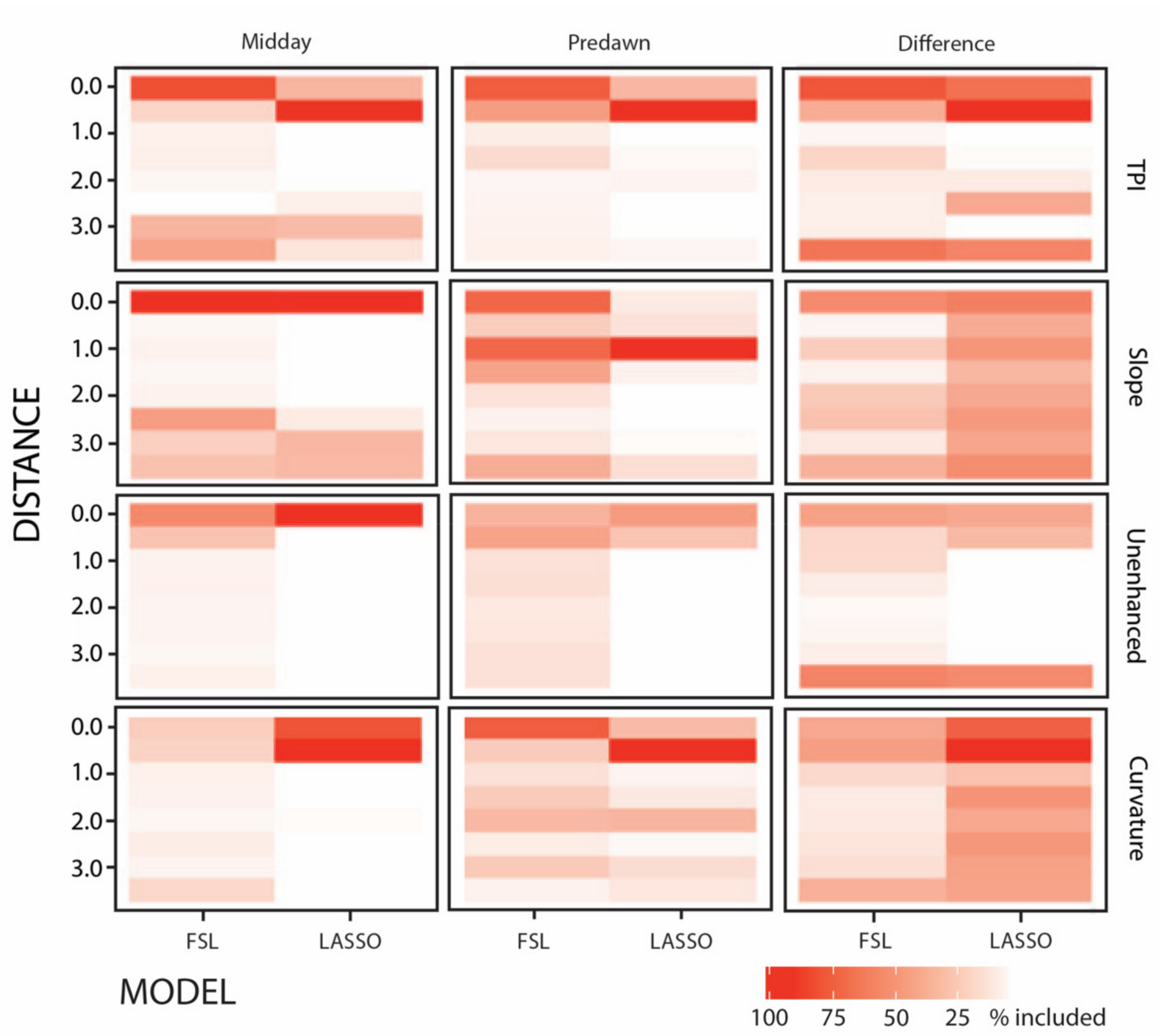
Given the large number of covariates used, and that developing a summary table of candidate models is both difficult to parse and interpret, we provide a graphical representation for discerning the most important covariates (Figure 6, Table 1). Overall, model selection procedures for both regression analyses produced a similar set of covariates. For predawn and midday imagery, covariates representing pixels at or near (0.5 m) each cave entrance were most useful for cave identification/prediction. Interestingly, LASSO often selected covariates describing conditions 0.5 m from the cave entrance, while FSL typically selected covariates describing conditions centered directly over the cave entrance (i.e., at 0 m). Analyses performed on the difference imagery covariates did not present a clear pattern for model selection. Our FSL models generated simpler, and thus more interpretable models, than LASSO. Subsequently, we developed a final predictive model based on the FSL results and included covariates that were selected in more than 50% of our simulations.
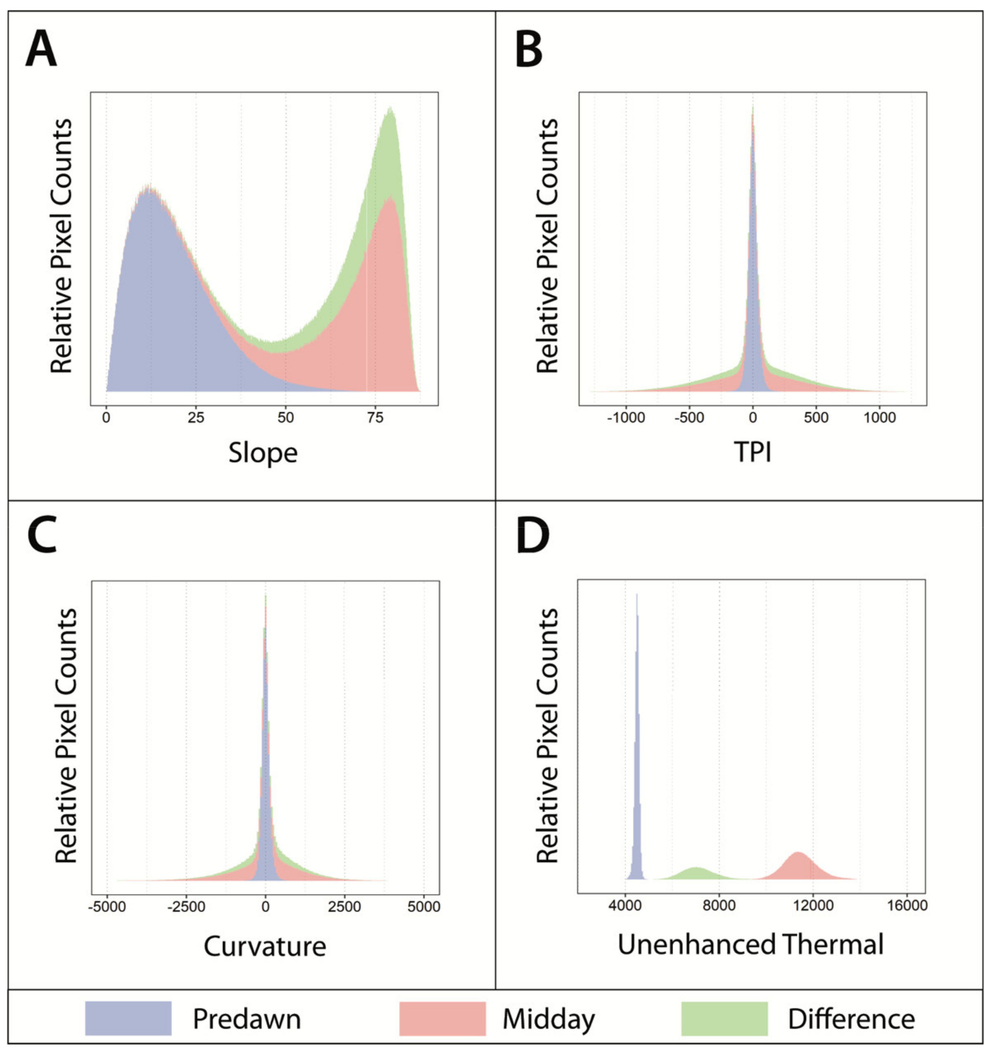
The following covariates were selected per imagery type: Predawn—slope, TPI, curvature at 0 m from cave entrance, as well as slope at 1 m from cave entrance; midday—slope, TPI, unenhanced thermal at 0 m from cave entrance; and 
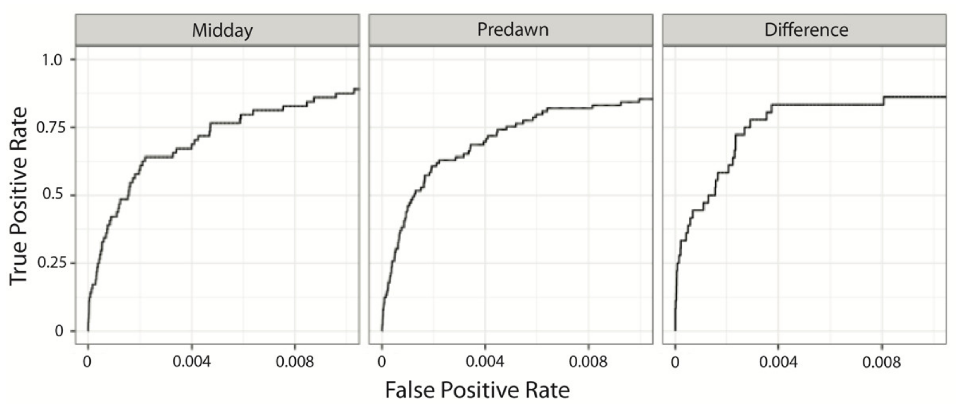
difference—TPI and slope at 0 m from cave entrance, as well as unenhanced thermal and TPI at 3.5 m from cave entrance. ROC curves for our final model had area under curve (AUC) values with 95% confidence intervals centered near 99% (predawn: (0.974, 0.998); midday: (0.994, 0.998); difference: (0.994, 0.999)). To examine the sensitivity of the variables included in our models, we varied the inclusion threshold between 30% and 70% and observed no practical difference in AUC values (Figure 7).
Our cluster analysis revealed that predawn and difference imagery resulted in the highest proportions of pixels representing known caves (both at 79%), while 55% of the pixels within the midday imagery represented known caves (Table 2). The total number of pixel clusters representing known caves were 47, 43, and 17 for predawn, midday, and difference imagery, respectively. Additionally, we identified 26, 29, and 8 clusters as either false positives or potential new cave entrances for the predawn, midday, and difference imagery, respectively. Examples of both known cave entrances and features with cave-like thermal behavior are provided in Figure 8.

4. Discussion

Through this work, we have demonstrated that applying techniques adapted from terrain analysis to thermal imagery holds significant promise for detecting caves. Across the three imagery types, combinations of slope, TPI, and curvature at 0 m from the cave entrance (i.e., the pixel at the approximate center of the cave’s entrance) were the variables included in the most parsimonious regression models. This suggests the use of terrain analysis algorithms is a robust tool to enhance detection capabilities with thermal imagery.
Overall, the models generated for predawn, midday, and difference performed similarly. We observed no quantitative differences in cave detection rates. ROC area under curves were 0.998, 0.997, and 0.996 for predawn, midday, and difference imagery datasets, respectively (refer to Figure 7). We also achieved an acceptable false positive rate (percent of non-cave pixels incorrectly identified as a cave) of approximately 0.02% when the true positive rate (percent of cave entrance pixels correctly identified as a cave) was between 20 and 50%. In other words, a 0.02% false positive rate implies that when examining a given region of one million pixels, we would have approximately 200 false positives while correctly identifying between 20 and 50% of the actual caves present.
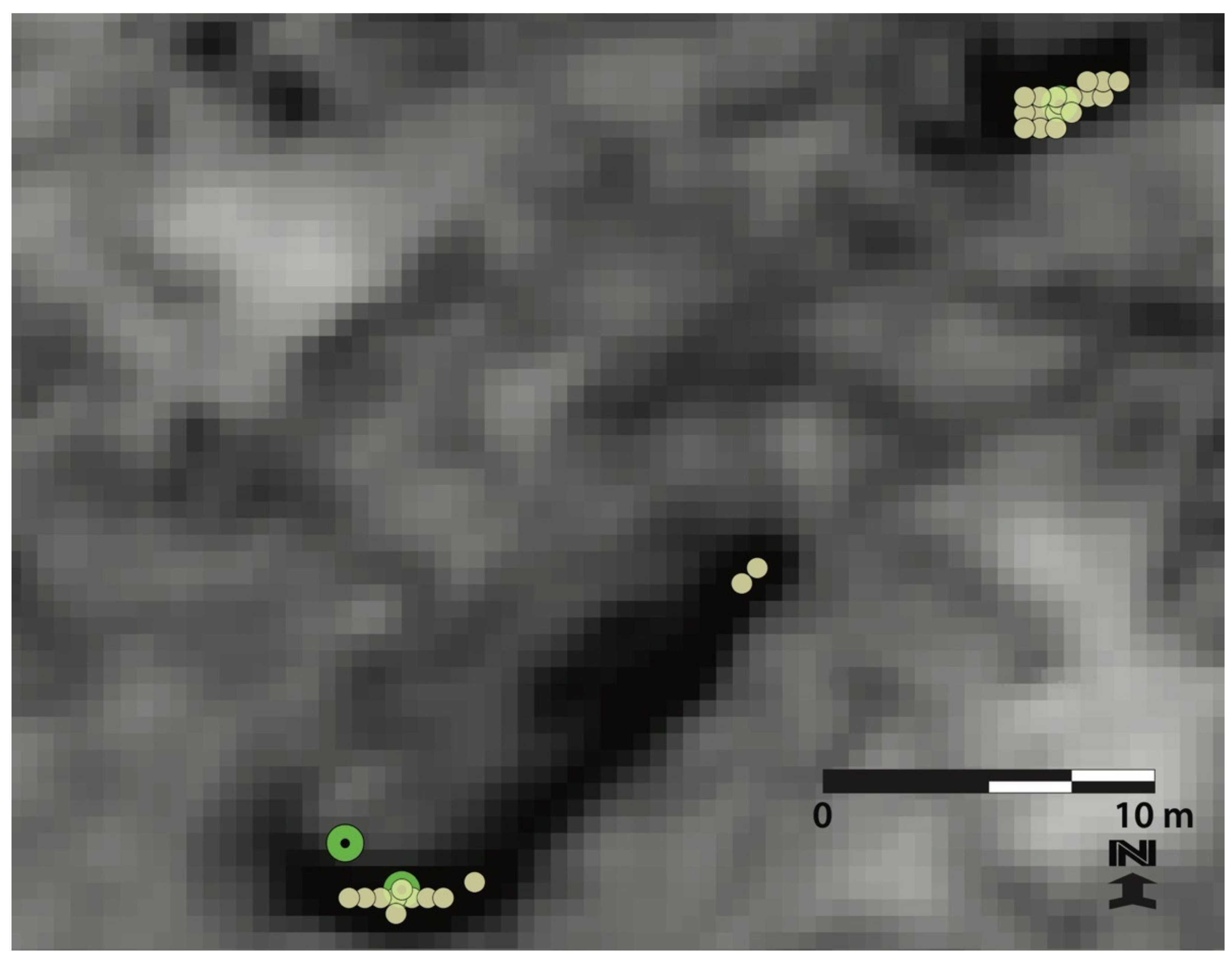
We observed a high degree of pixel aggregation centered on and around known cave locations. This phenomenon is influenced by imagery resolution, which affected the shape of the ROC curves. From our analysis, Figure 9 is an example of pixel aggregation where two of three clusters represented known caves. Given that our thermal imagery resolution was 0.5 m, and most cave entrances were meters in diameter (and thus represent multiple pixels), cluster analysis is a necessary step in imagery interpretation. Thus, identifying clusters of a small number of the highest-scoring pixels (i.e., those with the highest p ^ values) and then subsequently examining the visible imagery would be a good strategy for identifying potential false positives or small cave entrances or skylights. For terrestrial applications, a small number of aggregated pixels may represent a cave with a small entrance. This feature would likely become a high priority target for groundtruthing. For Mars, a small number of aggregated pixels representing a potential cave may be a low priority target for further examination as a human shelter or storage depot, but potentially a higher priority target for robotic exploration—as it may be more buffered from the surface environment (e.g., [96,97]). Thus, the grouping of pixels with cave-like thermal signatures into clusters will enable workers to prioritize which potential cave localities require further examination (i.e., physical groundtruthing of terrestrial caves or additional imagery interpretation for planetary caves).
As the difference imagery data layer performed similarly to predawn and midday imagery for the regression analysis, inclusion of this imagery type as part of the analytical framework may be considered unnecessary. However, analysis of the top-scoring 0.01% of the difference imagery identified the same high proportion of known caves as the predawn imagery (79%), although the lower p ^ max values suggest that the difference imagery in general performed poorly in capturing unique cave signatures.
However, we are hesitant to discount the utility of the difference imagery. Logically, this combined data layer had great potential. Its relatively unimpressive performance may have been due to smaller sample sizes (37 caves in the difference imagery compared to 64 and 89 caves in the midday and predawn imagery, respectively), and smaller analysis area (the overlap of midday and predawn imagery was 46% of the midday imagery and 36% of the predawn imagery). Furthermore, the warping and geometric transformations techniques employed to georeference the original images to the landscape almost certainly had some error. This error would have been compounded when we mosaicked multiple images into single midday and predawn images, and then the final difference image layer would have represented these compounded spatial errors. Subsequently, we suggest this introduced additionally noise into the analysis. With more accurately georeferenced images, we suspect the difference analysis would have performed much more favorably.
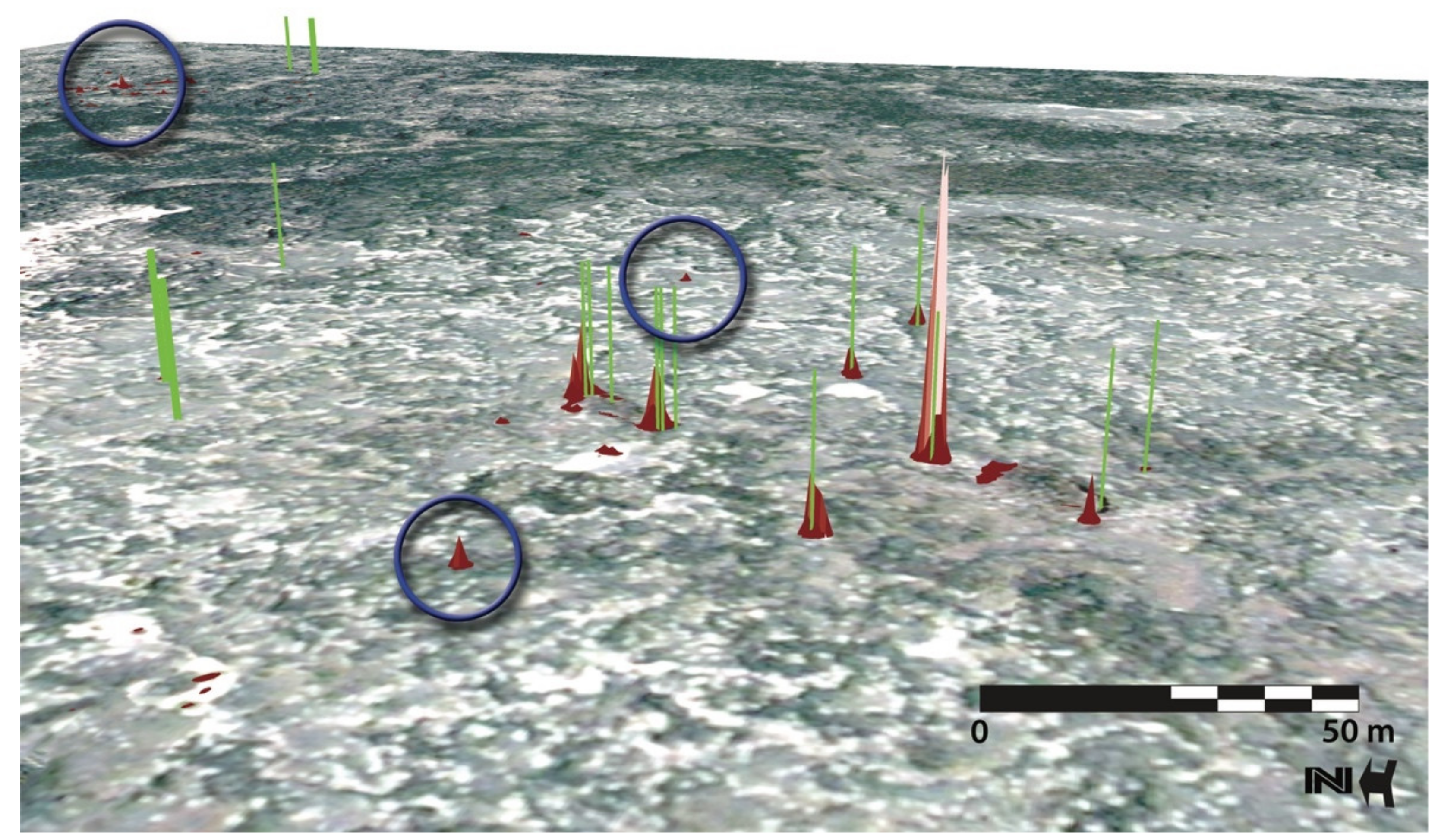
Our models show several distinct locations that exhibit thermal characteristics comparable to known cave entrances (Figure 8). The red peaks rising above the landscape correspond with cave-like thermal signatures. There are several other examples across the landscape with similar cave-like behavior but are not near any known caves; these features are either false positives, fissures, permanently shaded features, or undiscovered cave locations. These areas should ultimately be groundtruthed. A corresponding benefit of isolating the higher-probability sites is our ability to exclude large portions of the landscape as unlikely to be caves. Thus, we would be able to focus our examination of potential features of interest more efficiently.
Interestingly, a few known cave locations do not correspond with peaks on the probability surface, which raises the possibility that these caves may have some morphological or geometrical difference that changes their thermal signature. These features may be shallow caves with different thermal characteristics than actual cave entrances—the latter guided the development of our models. Alternatively, these thermally atypical features may occur in areas with different geologic material (i.e., loosely consolidated rock or soil), which is differentially influencing the thermal behavior within the immediate vicinity of the cave entrance. Further examination will be required to understand what sets them apart, as well as possibly developing models to capture their unique thermal signatures. These possibilities underscore the need to further examine these thermal signatures to potentially develop a method for organizing these features into categories. Once done, a groundtruthing effort may be undertaken, so that data may be collected to develop and test models that describe their thermal signatures.
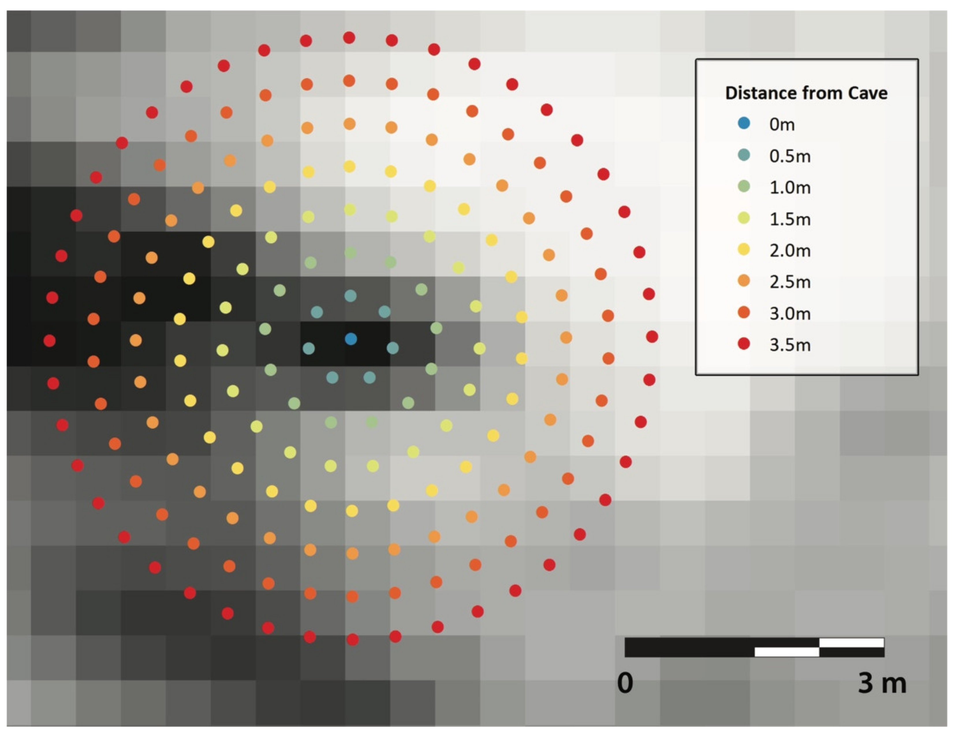
Because cave entrances are rarely perfectly circular, entrance configurations (often oval, oblong, crescent shaped or elongated cracks) may have skewed our values for most cave entrances. While our radial sampling method from the cave entrance (Figure 4) was both statistically and methodologically defensible and successful overall, in some cases we may have included pixels which are neither part of the cave entrance nor represent an area influenced by the cave entrance when we averaged values for a given feature. Selecting points in a radius from entrance may be extracting DN values in locations where surface temperatures are disproportionally influencing pixel values, which may have resulted in subpixel mixing [98]. It is also possible that we are extracting pixel values from surface locations where the thermal effects of the cave entrance were not influencing surface temperature. If this occurred, this would have skewed the average values for a given cave entrance. While the reality of imperfectly shaped cave entrances may have affected our results, we still differentiated known cave entrances from surface pixels regardless of cave entrance shape. However, a further refinement would be to visually examine each entrance (or suspected entrance) and then manually modify the pixel value extraction configuration to best fit the shape of the entrance of known or suspected cave entrances.
Generally, there are landscape conditions where caves may be either undetectable and/or the false positive rate may be high. Cave entrances occurring on north-facing slopes may be indistinguishable and lost due to topographic shadowing—as the DN values between these two features may be similar. Detection is also constrained by pixel resolution, such that cave entrances smaller than the pixel resolution may not be resolvable. Relying on one imagery type (e.g., predawn) could also increase the false positive rate as higher thermal inertia features, such as rock or bedrock outcrops, may be confused with cave entrances. Thus, acquiring imagery at two or more times over the 24-h cycle will be required to optimally improve detection capabilities under these conditions. Furthermore, poorly georeferenced thermal imagery may cause the cave locations to be shifted, or in particularly bad cases, may cause the predictive model to be based on skewed or warped data.
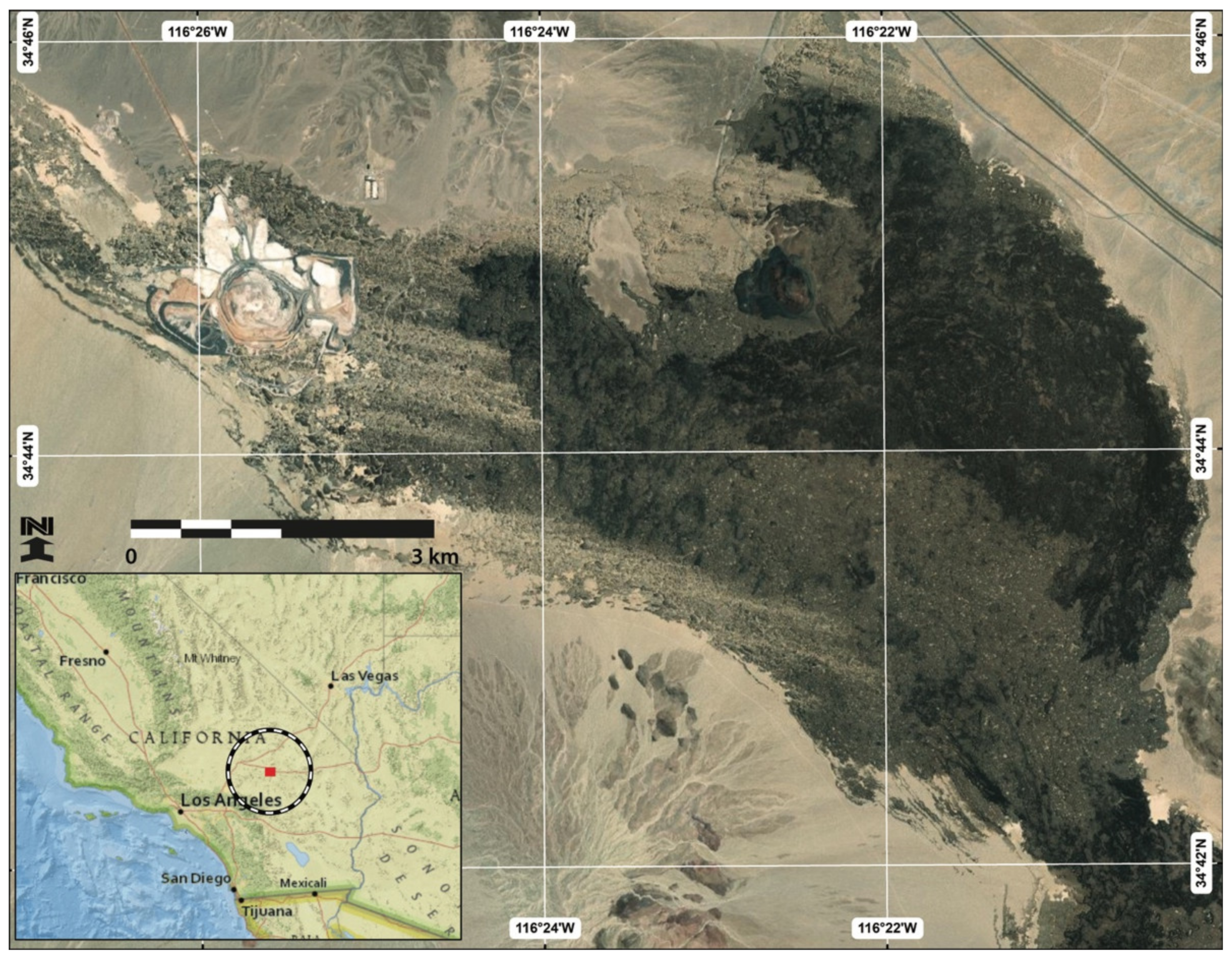
Overall, the identification and classification of non-cave landscape features that may be confused with cave entrances will be an important step towards further reducing the false positive rate. This becomes particularly relevant when examining possible cave features using only spacecraft-borne imagery of planetary bodies where a boots-on-the-ground groundtruthing effort is currently not possible. In the Pisgah dataset, we observed linear features (likely fissures), large collapse trenches, and areas of topographic shadowing. These features should be thoroughly examined. To further the science from both a terrestrial and planetary perspective, we could use this dataset as a feature class library. A first step would be to perform a supervised or unsupervised classification [99], or an object-based classification method to capture odd shapes on the landscape (e.g., [100,101,102]) within the thermal imagery. This would result in the development of feature categories, which then could be grouped based upon their likeness to one another; however, it is uncertain how these methods would perform in classifying the local thermal “shape” of the cave neighborhood. These procedures may require an intermediate step of describing shape metrics in a standard raster format before applying the classification methods. Thereafter, a field effort could be conducted to characterize and potentially reorganize these identified features into more specific categories. Once done, visible spectrum and thermal images of these features could be entered into a feature class library. These features could then be compared to similar features in both terrestrial and planetary imagery datasets. As this work progresses and more non-cave features with similar cave thermal signatures are identified, these data would be added to the feature class library.
Through applying the recommended methodological and field improvements elucidated above, this will enable us to further examine and hopefully quantify differences between deep and shallow caves, as well as identify and quantify those surface features, which may be confused with cave entrances. Through such an effort, we will further improve our ability to detect terrestrial and planetary caves—with the long-term goals of furthering cave conservation and management on Earth and identifying the best candidate cave sites for robotic exploration and human habitation on the moon, Mars and beyond.

5. Conclusions

We have shown that thermal imagery collected at least during predawn and midday are useful in detecting caves; other acquisition times may also be beneficial [69]. This finding has important implications for both terrestrial and planetary applications. As financial support continues to be one of the greatest challenges for biodiversity conservation efforts [103], the use of existing thermal imagery will factor prominently into budgeting cave research projects that may seek to detect caves for various conservation and management goals. For planetary missions, inherent difficulties often arise when attempting to acquire imagery from a specific region at a specific time from an orbiting or fly-by spacecraft. Thus, the flexibility illuminated through terrain analysis should expand the opportunities for detecting terrestrial and planetary caves using thermal imagery.
While the regression models for all three imagery types (predawn, midday, and difference) performed similarly, cluster analysis revealed that predawn and difference imagery out-performed midday imagery in identifying known cave entrance locations (see Table 2). This suggests that taking the time to develop and analyze difference imagery may be a worthwhile endeavor.
Finally, we emphasize the importance of cluster analysis as a necessary step for identifying and predicting cave locations. Overall, the number of pixels that look like a cave is less important than the groupings of these pixels. Thus, larger clusters of pixels may provide stronger evidence of a cave entrance.

Author Contributions

J.J.W., N.A.C. and T.N.T. conceived the study and secured funding. J.J. proposed the terrain analysis approach and led geospatial programming portion of research. D.L.S. lead statistical modeling in R. D.L.S., J.J. and J.J.W. discussed and developed statistical modeling frame. T.N.T. conducted calibration and atmospheric correction analysis. M.D.J. developed the QWIP thermal instrument and assisted with field data collection. J.J.W., N.A.C. and M.D.J. coordinated the overflight mission. All authors have read and agreed to the published version of the manuscript.

Funding

This study was supported by the NASA Astrobiology: Exobiology and Evolutionary Biology program under grant # EXOB07-0040 and NASA Goddard Space Flight Center.

Data Availability Statement

Data is available through the USGS ScienceBase Catalog (https://doi.org/10.5066/P9NF0L2I).

Acknowledgments

We are grateful for the assistance from the NASA Armstrong flight crew (Brittany Wells, Marty Trout, and Jacques Vachon) and the Pisgah ground crew (Doug Billings, Keith Muhlestein, Danny Hamlin, Cyril Johnson, Dave and Eleanor Larson, James Rice, and Lei Rowley) for coordinating data acquisition missions. Jim Shearer, the BLM-Barstow Field Office, facilitated issuance of research permits and supported this work. Russ Harter and Doug Billings, NSS Southern Cal Grotto, were instrumental in the identification of study caves and assisted with fieldwork. Edmond Grin and Jeff Moersch contributed to the development, execution, and success of the overall project. Much appreciation is extended to Laszlo Keszthelyi, David Mayer, Barbara Ralston, and two anonymous reviewers for providing comments leading to the improvement of this manuscript.

Conflicts of Interest

The authors declare no conflict of interest.

Appendix A. Precision and Accuracy Calculations of QWIP Thermal Instrument

The analysis of DN values in this paper depends on the precision and calibration stability of the instrument over the period of data collection and not the accuracy (i.e., calibration) of the data. Importantly, the analysis of DN levels acquired at different times of day (e.g., predawn and midday) is valid if the DN variation for each time-period is larger than the instrument precision, and the mean difference in DN between the two time periods is significantly larger than the variation of DN for the two times of day.
Titus et al. [69], using the same QWIP instrument, acquired two 24-h sets of oblique thermal images overlooking the Pisgah Lava Field from the approximate mid-elevation point on the Pisgah cinder cone in late March of 2010 [104]. In situ temperature data of both surface and near surface (~1 m AGL) atmosphere were acquired. They determined the precision of the brightness temperature (no correction for atmosphere or surface emissivity) was accurate to 1 °C. Based on this in situ calibration, which included atmospheric correction, they found surface temperature estimates were accurate to ~3.7 °C at 20 °C; this assumes an adequate characterization of the atmosphere, where air temperature and humidity data used may not accurately represent the conditions along the entire line-of-sight from camera to surface. They asserted this was likely the cause for the larger uncertainty in accuracy under field conditions, when compared to laboratory testing results. Refer to Titus et al. [69] for more details.
For the 2011 overflight data, no reliable surface or air temperature data were acquired. The calibration of the QWIP, which depends on the “Non-Uniformity Correction” setting was changed between the 2010 and 2011 QWIP campaigns. Therefore, we do not have absolute calibration coefficients. However, as previously mentioned, the technique presented in this paper only depends on the instrument data having high precision and the calibration remaining stable during the campaign. To increase our confidence, we present a comparison between the 2010 and 2011 datasets, as shown in Figure A1. Calibration curves assume atmospheric conditions as determined from PRISM data [105] and Humidity Converter [106] (see Table A1) and line-of-sight distance being the mean overflight altitude. Two sets of atmospheric conditions are shown for predawn and midday flight times. Surface radiance was corrected for atmospheric absorption and emission sensu Titus et al. [69]. The three sets of calibration coefficients from Titus et al. [69] are shown in Table A2. DN offset was increased by 4500 DN, while the calibration gain was unchanged. Surface emissivity was assumed to be 0.72, consistent with basalt. Box plots in Figure A1 show DN distributions for predawn (bottom left) and midday (upper right) for the overflight data (Table A3) and surface temperatures of the 11 sample sites for the 2010 study (Table A4). While surface temperature statistics are from the previous year and a few weeks earlier in the spring, close alignment of observed DN values and surface temperatures provided a confidence check that the QWIP continued to be a precision instrument with stable calibration over the period of the 2011 overflight campaign. The offset of the midday box plot could be due to an increase in gain from 2010, slightly higher surface temperatures (being early April and not late March), or both.
Flight times were selected to maximize the temperature difference between the two overflights while minimizing temperature changes during each overflight. Selection of flight times were based on the analysis of the 2010 data [104]. For the 11 sample sites where surface temperature was measured, the difference between minimum and maximum temperatures (temperature range) varied between 3.2 °C and 6.1 °C for the midday flight time span and between 0.9 °C and 2.1 °C for the predawn flight time span (Table A5). Temperature fluctuations should have a negligible effect on spatial indices calculated for either midday or predawn mosaics as the adjacent pixels would have been collected at the same time. For indices that utilize the difference between midday and predawn DN levels, temperature fluctuation may introduce additional uncertainty but the smallest difference in temperature for the 2010 data was 19 °C, which is easily discernable from the maximum variations observed during each overflight time span.
Acquisition of aircraft borne thermal imagery takes time, over which the surface temperature changes. In this paper, thermal indices generated from either midday or predawn flights were used for the orthorectified images, where all pixels were collected at the same local time. Because these indices were based on differences and not absolute DN values, these indices are relatively invariant to surface changes during each few-hour flight. Indices based on DN differences between midday and predawn flights must compare the mosaics, which do have variations in local time, and therefore changes in surface temperature. However, the expected DN changes over the time of flight is smaller than the DN gap between midday and predawn flights. This gap is apparent in both Figure A1 and Table A5. By selecting these two times of flight, we maximized the DN differences between the two overflight mosaics, while minimizing DN variations within each mosaic. Thus, the results presented in this paper should be robust.
Table A1. 2011 overflight atmospheric conditions with air temperature and dew point estimated using PRISM data [105].
OverflightDateTimes (PDT)Air TempDew PointRHH (mm/km)Absorption
Midday11 APR 12:22–14:5720.02 °C−3.71 °C19.9%2.960.0639169
Predawn13 APR 04:26–06:498.22° C0.37° C57.71%4.160.0886765
Table A2. Calibration coefficients from 2010 experiments [69] to roughly match observations and assumptions. Calibration offset has been increased by 4500 DN from Titus et al. [69].
Region of InterestCalibration OffsetCalibration Gain
B Cave−4227.041864.02
Station 7 trench−6021.12077.23
Combined−4804.051838.57
Table A3. 2011 overflight DN statistics.
OverflightCountMinMaxMedianMeanSD
Midday1,363,990812716,05211,42311,458.59710.8345
Predawn1,637,5862656533745004,494.94992.8291
Table A4. 2010 Pisgah surface temperature statistics. Surface temperatures (in degrees Celsius) as estimated by Titus et al. [69] for the 11 sample locations, which were combined to determine statistics. Number (#) of data points is the number of temperature values taken at five-minute intervals from the 11 samples sites within the overflight time span. Minimum, maximum, median, mean, and standard deviation (SD) were derived from these temperature values.
Overflight#_Data PointsMinMaxMedianMeanSD
Midday34131.178548.308538.851239.15044.16746
Predawn3085.2913311.71888.897958.511861.70285
Table A5. Surface temperature (in degrees Celsius) and image DN range values from the 11 sample sites where surface temperature data were collected in 2010 [69,104]. Sample Site numbers (#) ranges from 1 to 11. Refer to Table A1 for flight times. DN gaps between midday minimum and predawn maximum DN levels are shown for comparison.
RangeSample Site #Mean
1234567891011
Midday (C)4.53.63.24.55.74.33.36.14.04.24.24.3
Predawn (C)1.52.10.91.51.81.11.01.91.51.51.51.5
Midday (DN)953555109483891077493912171426125713561029
Predawn (DN)261273273368342264258281270260253282.1
DN Midday-Predawn Gap (DN)547652294872552851505220507755615218498853455242.2
Figure A1. Calibration curves estimated using the coefficients from Titus et al. [69] but adjusted for the Pisgah 2011 dataset. Red, blue, and black curves are based on the calibration coefficients derived from the B Cave, Station 7 trench, and combined datasets as shown in Table A2. Solid and dashed lines are for predawn and midday atmospheric conditions, respectively. Box plots show the comparison between 2011 DN range of values (Table A3) and the 2010 surface temperature range of values (Table A4). Top and bottom of vertical line (or whisker) represent maximum and minimum DN values, while upper and lower horizontal lines of the box represent the upper and lower quartiles for DN values; horizontal line within the box is the median DN value. Horizontal whisker, vertical bounding lines of boxes, and the vertical line at center represent minimum and maximum surface temperatures, upper and lower quartiles of surface temperature, and median surface temperature, respectively. Note: Box plot at bottom right is small due to low variation in predawn DN levels; thus, the box appears filled. Instrument bias has been increased by 4500 DN. The gain was not adjusted as we cannot determine if the April 2011 surface temperatures were higher or if the gain factor was slightly higher. It is likely that both occurred. A distinct gap for both surface temperature and measured DN levels exists between the midday and predawn data, suggesting that “topographical” indices that depend on midday and predawn differences should be robust even with some variation in surface temperatures during the overflight times.
Remotesensing 13 03578 g0a1

References

  1. Wynne, J.J.; Titus, T.N.; Diaz, G.C. On Developing Thermal Cave Detection Techniques for Earth, the Moon and Mars. Earth Planet. Sci. Lett. 2008, 272, 240–250. [Google Scholar] [CrossRef]
  2. Froschauer, A.; Coleman, J. North American Bat Death Toll Exceeds 5.5 Million from White-Nose Syndrome. US Fish and Wildlife Service News Release. 2012. Available online: https://www.fws.gov/news/ShowNews.cfm?ID=0DA47708-D93C-21F4-3AA3E6EEB217DAA0 (accessed on 15 June 2018).
  3. Haman, K.; Hibbard, C.; Lubeck, M. Bat with White-Nose Syndrome Confirmed in Washington State; Washington Department of Fish and Wildlife: Olympia, WA, USA, 2016. Available online: http://wdfw.wa.gov/news/mar3116b/ (accessed on 23 September 2017).
  4. O’Driscoll, P.; Verant, M.; MacKay, R.; Hibbard, C.; Abernethy, I. Fungus That Causes White-Nose Syndrome in Bats Detected in Wyoming for the First Time, Multiagency News Release, 01 June 2018. 2018. Available online: https://www.whitenosesyndrome.org/sites/default/files/files/fola_-_pd_fungus_-_wy-nps-fws_release_final_-_06_01_2018_1.pdf (accessed on 15 June 2018).
  5. Wynne, J.J. White-Nose Syndrome Decontamination Procedures for Backcountry Subterranean Projects. Park Sci. 2017, 33, 50–62. [Google Scholar]
  6. Reddell, J.R. A Review of the Cavernicole Fauna of Mexico, Guatemala, and Belize. Bull. Tex. Meml. Mus. 1981, 591, 1–327. [Google Scholar]
  7. Culver, D.C.; Master, L.L.; Christman, M.C.; Hobbs, H.H., III. Obligate Cave Fauna of the 48 Contiguous United States. Conserv. Biol. 2000, 14, 386–401. [Google Scholar] [CrossRef]
  8. Christman, M.C.; Culver, D.C.; Madden, M.K.; White, D. Patterns of Endemism of the Eastern North American Cave Fauna. J. Biogeogr. 2005, 32, 1441–1452. [Google Scholar] [CrossRef]
  9. Deharveng, L. Mulun and Surrounding Karsts (Guangxi) Host the Richest Cave Fauna of China. Subterr. Biol. Verona 2008, 6, 75–79. [Google Scholar]
  10. Harvey, M.S.; Wynne, J.J. Troglomorphic Pseudoscorpions (Arachnida: Pseudoscorpiones) of Northern Arizona, with the Description of Two New Short-Range Endemic Species. J. Arachnol. 2014, 42, 205–219. [Google Scholar] [CrossRef]
  11. Harvey, M.S.; Rix, M.G.; Framenau, V.W.; Hamilton, Z.R.; Johnson, M.S.; Teale, R.J.; Humphreys, G.; Humphreys, W.F. Protecting the Innocent: Studying Short-Range Endemic Taxa Enhances Conservation Outcomes. Invertebr. Syst. 2011, 25, 1–10. [Google Scholar] [CrossRef]
  12. Shear, W.A.; Taylor, S.J.; Wynne, J.J.; Krejca, J.K. Cave Millipeds of the United States. VIII. New Genera and Species of Polydesmidan Millipeds from Caves in the Southwestern United States (Diplopoda, Polydesmida, Macrosternodesmidae). Zootaxa 2009, 2151, 47–65. [Google Scholar]
  13. Tian, M. A New Subgenus and Two New Species of the Troglobitic Genus Dongodytes Deuve from Guangxi, China (Coleoptera, Carabidae). Subterr. Biol. 2011, 8, 57–64. [Google Scholar] [CrossRef]
  14. Borges, P.A.V.; Cardoso, P.; Amorim, I.R.; Pereira, F.; Constância, J.P.; Nunes, J.C.; Barcelos, P.; Costa, P.; Gabriel, R.; Dapkevicius, M.L. Volcanic Caves: Priorities for Conserving the Azorean Endemic Troglobiont Species. Int. J. Speleol. 2012, 41, 101–112. [Google Scholar] [CrossRef] [Green Version]
  15. Niemiller, M.L.; Zigler, K.S. Patterns of Cave Biodiversity and Endemism in the Appalachians and Interior Plateau of Tennessee, USA. PLoS ONE 2013, 8, e64177. [Google Scholar] [CrossRef]
  16. Mitchell, R. Total Number and Density Estimates of Some Species of Cavernicoles Inhabiting Fern Cave, Texas. Annales de Spéléologie 1970, 25, 73–90. [Google Scholar]
  17. Niemiller, M.L.; Zigler, K.S.; Ober, K.A.; Carter, E.T.; Engel, A.S.; Moni, G.; Philips, T.K.; Stephen, C.D. Rediscovery and Conservation Status of Six Short-Range Endemic Pseudanophthalmus Cave Beetles (Carabidae: Trechini). Insect Conserv. Divers. 2017, 10, 495–501. [Google Scholar] [CrossRef]
  18. Wynne, J.J.; Shear, W.A. A New Millipede, Austrotyla Awishoshola, n. sp. (Diplopoda, Chordeumatida, Conotylidae) from New Mexico, USA, and the Importance of Cave Moss Gardens as Refugial Habitats. Zootaxa 2016, 4084, 285–292. [Google Scholar] [CrossRef]
  19. Bernard, C.; Wynne, J.J. Disparrhopalites Naasaveqw n. sp. from Caves at Wupatki National Monument, Arizona, Synonymy of Dietersminthurus Palacios-Vargas, Cuéllar & Vázquez, 1998 with Disparrhopalites Stach, 1956 and Composition of Songhaicinae (Collembola: Sminthuridae). Zootaxa 2017, 4319, 77–90. [Google Scholar]
  20. Benedict, E.M. A New Species of Apochthonius Chamberlin from Oregon (Pseudoscorpionida, Chthoniidae). J. Arachnol. 1979, 7, 79–83. [Google Scholar]
  21. Jureková, N.; Raschmanová, N.; Miklisová, D.; Kováč, L. Mesofauna at the Soil-Scree Interface in a Deep Karst Environment. Diversity 2021, 13, 242. [Google Scholar] [CrossRef]
  22. Marcin, M.; Raschmanová, N.; Miklisová, D.; Kováč, L. Microclimate and Habitat Heterogeneity as Important Drivers of Soil Collembola in a Karst Collapse Doline in the Temperate Zone. Invertebr. Biol. 2021, e12315. [Google Scholar]
  23. Wynne, J.J.; Bernard, E.C.; Howarth, F.G.; Sommer, S.; Soto-Adames, F.N.; Taiti, S.; Mockford, E.L.; Horrocks, M.; Pakarati, L.; Pakarati-Hotus, V. Disturbance Relicts in a Rapidly Changing World: The Rapa Nui (Easter Island) Factor. BioScience 2014, 64, 711–718. [Google Scholar] [CrossRef] [Green Version]
  24. Bernard, E.C.; Soto-Adames, F.N.; Wynne, J.J. Collembola of Rapa Nui (Easter Island) with Descriptions of Five Endemic Cave-Restricted Species. Zootaxa 2015, 3949, 239–267. [Google Scholar] [CrossRef]
  25. Taiti, S.; Wynne, J.J. The Terrestrial Isopoda (Crustacea, Oniscidea) of Rapa Nui (Easter Island), with Descriptions of Two New Species. ZooKeys 2015, 515, 27–49. [Google Scholar] [CrossRef] [Green Version]
  26. Culver, D.C.; Sket, B. Hotspots of Subterranean Biodiversity in Caves and Wells. J. Cave Karst Stud. 2000, 62, 11–17. [Google Scholar]
  27. Parness, A.; Frost, M.; Thatte, N.; King, J.P. Gravity-Independent Mobility and Drilling on Natural Rock Using Microspines. In Proceedings of the 2012 IEEE International Conference on Robotics and Automation, Saint Paul, MN, USA, 12–14 May 2012; pp. 3437–3442. [Google Scholar]
  28. Kerber, L.; Nesnas, I.; Ashley, J.; Malaska, M.; Parcheta, C.; Mitchell, K.; Anderson, R. Exploring Pits and Caves with the Axel Extreme Terrain Rover. In Proceedings of the 2nd International Planetary Caves Conference, Flagstaff, AZ, USA, 20–23 October 2015; Volume 1883, p. 9022. [Google Scholar]
  29. Wynne, J.J. The Scientific Importance of Caves in Our Solar System. NSS News, 1 March 2016. [Google Scholar]
  30. Titus, T.N.; Phillips-Lander, C.; Boston, P.; Wynne, J.J.; Kerber, L. Planetary Cave Exploration Progresses. Eos. Earth Space Sci. News 2020, 101. [Google Scholar] [CrossRef]
  31. Titus, T.N.; Wynne, J.J.; Boston, P.; de León, P.; Demirel-Floyd, C.; Jones, H.; Sauro, F.; Uckert, K.; Aghamohammadi, A.; Alexander, C.; et al. Science and Technology Requirements to Explore Caves in Our Solar System. Bull. Am. Astron. Soc. 2021, 53, 167. [Google Scholar]
  32. Boston, P.; Frederick, R.; Welch, S.; Werker, J.; Meyer, T.; Sprungman, B.; Hildreth-Werker, V.; Thompson, S.; Murphy, D. Human Utilization of Subsurface Extraterrestrial Environments. Gravit. Space Res. 2007, 16, 121–131. [Google Scholar]
  33. Al Husseini, A.M.; Alvarez Sanchez, L.; Antonakopoulos, K.; Apeldoorn, J.J.; Ashford, K.L., Jr.; Atabay, K.D.; Langston, S. Access Mars: Assessing Cave Capabilities Establishing Specific Solutions. International Space University, Final Report. Pace Studies Program Class of 2009. ISS, Illkirch-Graffenstaden, France. 2009. Available online: https://commons.erau.edu/publication/1232/ (accessed on 6 September 2021).
  34. Wynne, J.J.; Titus, T.N.; Boston, P.J. Planetary Caves’ Role in Astronaut Bases and the Search for Life. Eos. Earth Space Sci. News 2016, 97. [Google Scholar] [CrossRef]
  35. Cushing, G. Mars Global Cave Candidate Catalog (MGC3). In Proceedings of the Astrobiology Science Conference, Mesa, AZ, USA, 24–28 April 2017; p. 3708. [Google Scholar]
  36. Cushing, G.; Titus, T.N.; Wynne, J.J.; Christensen, P. THEMIS Observes Possible Cave Skylights on Mars. Geophys. Res. Lett. 2007, 34, L17201. [Google Scholar] [CrossRef] [Green Version]
  37. Haruyama, J.; Hioki, K.; Shirao, M.; Morota, T.; Hiesinger, H.; van der Bogert, C.H.; Miyamoto, H.; Iwasaki, A.; Yokota, Y.; Ohtake, M.; et al. Possible Lunar Lava Tube Skylight Observed by SELENE Cameras. Geophys. Res. Lett. 2009, 36, L21206. [Google Scholar] [CrossRef] [Green Version]
  38. Wagner, R.V.; Robinson, M.S. Distribution, Formation Mechanisms, and Significance of Lunar Pits. Icarus 2014, 237, 52–60. [Google Scholar] [CrossRef] [Green Version]
  39. Wagner, R.; Robinson, M. Update: The Search for Lunar Pits. In Proceedings of the 2nd International Planetary Caves Conference, Flagstaff, AZ, USA, 20–23 October 2015; Volume 1883, p. 9021. [Google Scholar]
  40. Wagner, R.; Robinson, M. Occurrence and Origin of Lunar Pits: Observations from a New Catalog. In Proceedings of the Lunar and Planetary Science Conference, League City, TX, USA, 15–19 March 2021; p. 2530. [Google Scholar]
  41. Hansen, C.; Shemansky, D.E.; Esposito, L.W.; Stewart, A.; Lewis, B.; Colwell, J.; Hendrix, A.; West, R.A.; Waite, J., Jr.; Teolis, B.; et al. The Composition and Structure of the Enceladus Plume. Geophys. Res. Lett. 2011, 38, L11202. [Google Scholar] [CrossRef] [Green Version]
  42. Porco, C.; DiNino, D.; Nimmo, F. How the Geysers, Tidal Stresses, and Thermal Emission across the South Polar Terrain of Enceladus Are Related. Astron. J. 2014, 148, 45. [Google Scholar] [CrossRef] [Green Version]
  43. Geissler, P.; McMillan, M. Galileo Observations of Volcanic Plumes on Io. Icarus 2008, 197, 505–518. [Google Scholar] [CrossRef] [Green Version]
  44. Roth, L.; Saur, J.; Retherford, K.D.; Strobel, D.F.; Feldman, P.D.; McGrath, M.A.; Nimmo, F. Transient Water Vapor at Europa’s South Pole. Science 2014, 343, 171–174. [Google Scholar] [CrossRef]
  45. Duxbury, N.; Brown, R. The Role of an Internal Heat Source for the Eruptive Plumes on Triton. Icarus 1997, 125, 83–93. [Google Scholar] [CrossRef]
  46. Wynne, J.J.; Titus, T.N.; Agha-Mohammadi, A.; Azua-Bustos, A.; Boston, P.J.; de León, P.; Demirel-Floyd, C.; De Waele, J.; Jones, H.; Miller, A.Z.; et al. Fundamental Science and Engineering Questions in Planetary Cave Exploration. J. Geophys. Res. Planets 2021. in review. [Google Scholar]
  47. Wynne, J.J.; Titus, T.N.; Jhabvala, M.; Cushing, G.; Cabrol, N.; Grin, E. Distinguishing Caves from Non-Cave Anomalies Using Thermal Infrared: Lessons for the Moon and Mars. In Proceedings of the Lunar and Planetary Science Conference, League City, TX, USA, 23–27 March 2009; p. 2451. [Google Scholar]
  48. Newcomer, K.; Moersch, J.; Cabrol, N.; Grin, E.; Wynne, J.J.; Chojnacki, M. Evalution of a Proposed Technique for Identifying Martian Caves in THEMIS Infrared Images. In Proceedings of the Lunar and Planetary Science Conference, League City, TX, USA, 7–11 March 2011; p. 2739. [Google Scholar]
  49. Howarth, F.G. The Zoogeography of Specialized Cave Animals: A Bioclimatic Model. Evolution 1980, 34, 394–406. [Google Scholar] [CrossRef] [PubMed]
  50. Howarth, F.G. Bioclimatic and Geologic Factors Governing the Evolution and Distribution of Hawaiian Cave Insects. Entomol. Gen. 1982, 8, 17–26. [Google Scholar] [CrossRef]
  51. Badino, G. Cave Temperatures and Global Climatic Change. Int. J. Speleol. 2004, 33, 103–114. [Google Scholar] [CrossRef]
  52. Perrier, F.; Le Mouël, J.-L.; Richon, P. Spatial and Temporal Dependence of Temperature Variations Induced by Atmospheric Pressure Variations in Shallow Underground Cavities. Pure Appl. Geophys. 2010, 167, 253–276. [Google Scholar] [CrossRef]
  53. Luetscher, M.; Lismonde, B.; Jeannin, P.-Y. Heat Exchanges in the Heterothermic Zone of a Karst System: Monlesi Cave, Swiss Jura Mountains. J. Geophys. Res. Earth Surf. 2008, 113, F02025. [Google Scholar] [CrossRef] [Green Version]
  54. Neugebauer, G.; Münch, G.; Kieffer, H.; Chase, S., Jr.; Miner, E. Mariner 1969 Infrared Radiometer Results: Temperatures and Thermal Properties of the Martian Surface. Astron. J. 1971, 76, 719–749. [Google Scholar] [CrossRef] [Green Version]
  55. Byrne, G.; Davis, J. Thermal Inertia, Thermal Admittance, and the Effect of Layers. Remote Sens. Environ. 1980, 9, 295–300. [Google Scholar] [CrossRef]
  56. Rinker, J. Airborne Infrared Thermal Detection of Caves and Crevasses. Photogramm. Eng. Remote. Sens. 1975, 44, 1391–1400. [Google Scholar]
  57. Wynne, J.J.; Titus, T.N.; Drost, C.; Toomey, R.; Peterson, K. Annual Thermal Amplitudes and Thermal Detection of Southwestern US. Caves: Additional Insights for Remote Sensing of Caves on Earth and Mars. In Proceedings of the Lunar and Planetary Science Conference, League City, TX, USA, 10–14 March 2008; p. 2459. [Google Scholar]
  58. Wynne, J.J.; Jhabvala, M.; Wells, B.; Trout, M.; Decker, D.; Ruby, D.R.; Muhlestein, K.; Billings, D.; Rice, J.; Taylor, B.; et al. Aircraftborne Thermal and Visible Imagery Acquisition and Ground Data Instrument Recovery of Caves, Mojave Desert, California. Explorers Club Flag Report (Flag # 139). On file at The Explorers Club, New York, NY, USA. 2011. Available online: https://explorers.org/pdf/Flag_139_-_J._Judson_Wynne_2011_Mojave_6-17-11.pdf (accessed on 2 July 2021).
  59. Titus, T.N.; Wynne, J.J.; Jhabvala, M.; Cushing, G.; Cabrol, N. Cave Detection Using Oblique Thermal Imaging. In Proceedings of the First International Planetary Caves Workshop, Carlsbad, NM, USA, 25–28 October 2011; p. 1640. [Google Scholar]
  60. Groemer, G.; Foresta, L.; Turetschek, T.; Bothe, C.; Boyd, A.; Dinkelaker, A.; Dissertori, M.; Fasching, D.; Fischer, M.; Föger, D.; et al. A Case for Using Ground-Based Thermal Inertia Measurements to Detect Martian Caves. Astrobiology 2014, 14, 431–437. [Google Scholar] [CrossRef]
  61. Jhabvala, M.; Choi, K. Evolution of QWIP Focal Plane Development at the NASA/Goddard Space Flight Center. In Proceedings of the Quantum Sensing and Nanophotonic Devices IX International Society for Optics and Photonics, San Francisco, CA, USA, 22–26 January 2012; Volume 8268, p. 82682. [Google Scholar]
  62. Wise, W.S. Origin of Basaltic Magmas in the Mojave Desert Area, California. Contrib. Mineral. Petrol. 1969, 23, 53–64. [Google Scholar] [CrossRef]
  63. Harter, R. Pisgah! In Proceedings of the Western Region, National Speleological Society-Speleo-Ed Seminar, Rainbow Basin-Barstow, California, CA, USA, 12–14 May 2009; pp. 20–22. [Google Scholar]
  64. Hardgrove, C.; Moersch, J.; Whisner, S. Thermal Imaging of Alluvial Fans: A New Technique for Remote Classification of Sedimentary Features. Earth Planet. Sci. Lett. 2009, 285, 124–130. [Google Scholar] [CrossRef]
  65. Hardgrove, C.; Moersch, J.; Whisner, S. Thermal Imaging of Sedimentary Features on Alluvial Fans. Planet. Space Sci. 2010, 58, 482–508. [Google Scholar] [CrossRef]
  66. Montanaro, M.; Reuter, D.C.; Markham, B.L.; Thome, K.J.; Lunsford, A.W.; Jhabvala, M.D.; Rohrbach, S.O.; Gerace, A.D. Spectral Analysis of the Primary Flight Focal Plane Arrays for the Thermal Infrared Sensor. In Proceedings of the Algorithms and Technologies for Multispectral, Hyperspectral, and Ultraspectral Imagery XVII. International Society for Optics and Photonics, Orlando, FL, USA, 11 May 2021; Volume 8048, p. 804816. [Google Scholar]
  67. [NASA] National Aeronautics and Space Administration. In Technology Readiness Level; 2021. Available online: https://www.nasa.gov/directorates/heo/scan/engineering/technology/technology_readiness_level (accessed on 15 July 2021).
  68. QmagiQ, LLC Handheld Longwave Infrared Camera Based on Highly Sensitive Quantum Well Infrared Photodetectors, Phase 1 Final Report; NASA Small Business Innovative Research: Nashua, NH, USA, 2007.
  69. Titus, T.N.; Wynne, J.J.; Jhabvala, M.D.; Cabrol, N. Using Near–Surface Temperature Data to Calibrate High-Resolution Thermal Infrared Imagery and Estimate Physical Surface Properties. MethodsX 2021. in review. [Google Scholar]
  70. Wynne, J.J.; Jenness, J.; Sonderegger, D.L.; Jhabvala, M.D. Terrain Analysis of Thermal Imagery for Terrestrial Cave Detection; NASA Goddard Space Flight Center: Greenbelt, MD, USA, 2016; p. 135.
  71. U.S. Geological Survey The National Map, 3DEP Products and Services. 2018. Available online: https://www.usgs.gov/core-science-systems/ngp/3dep/data-tools (accessed on 12 June 2018).
  72. ArcGIS REST Services Directory. 2021. Available online: https://services.arcgisonline.com/ArcGIS/rest/services/World_Imagery/MapServer/4 (accessed on 2 July 2021).
  73. USDA Farm Service Agency NAIP Imagery. 2018. Available online: https://www.fsa.usda.gov/programs-and-services/aerial-photography/imagery-programs/naip-imagery/ (accessed on 8 June 2018).
  74. Esri. Fundamentals of Georeferencing a Raster Dataset. 2017. Available online: http://desktop.arcgis.com/en/arcmap/10.3/manage-data/raster-and-images/fundamentals-for-georeferencing-a-raster-dataset.htm (accessed on 13 January 2017).
  75. Taigman, Y.; Yang, M.; Ranzato, M.; Wolf, L. Deepface: Closing the Gap to Human-level Performance in Face Verification. In Proceedings of the IEEE conference on Computer Vision and Pattern Recognition, Columbus, OH, USA, 28 June 2014; pp. 1701–1708. [Google Scholar]
  76. Microsoft Microsoft/USBuildingFootprints on GitHub. 2018. Available online: https://github.com/Microsoft/USBuildingFootprints (accessed on 25 July 2018).
  77. Weiss, A. Topographic Position and Landforms Analysis. Proceedings of the ESRI User Conference, San Diego, CA, USA, 13 October 2021; Available online: http://www.jennessent.com/arcview/TPI_Weiss_poster.htm (accessed on 5 February 2017).
  78. Jenness, J. Topographic Position Index (TPI) v. 1.2. Jenness Enterprises, Flagstaff, AZ, USA. 2006. Available online: http://www.jennessent.com/downloads/TPI_Documentation_online.pdf (accessed on 6 February 2017).
  79. Horn, B.K.P. Hill Shading and the Reflectance Map. Proc. IEEE 1981, 69, 14–47. [Google Scholar] [CrossRef] [Green Version]
  80. Burrough, P.A.; McDonnell, R.A. Principles of Geographical Information Systems; Oxford University Press: Oxford, USA, 1998; ISBN 0-19-823365-5. [Google Scholar]
  81. Zevenbergen, L.W.; Thorne, C.R. Quantitative Analysis of Land Surface Topography. Earth Surf. Process. Landf. 1987, 12, 47–56. [Google Scholar] [CrossRef]
  82. Emerson, J.D.; Stoto, M.A. Transforming Data. In Understanding Robust and Exploratory Data Analysis; Hoaglin, D.C., Hosteler, F., Tukey, J.W., Eds.; John Wiley & Sons: Hoboken, NJ, USA, 1983; pp. 97–128. [Google Scholar]
  83. Bajaj, C.L. Splines and geometric modeling. In Handbook of Discrete and Computational Geometry; Toth, C.D., O’Rourke, J., Goodman, J.E., Eds.; CRC Press: Boca Raton, FL, USA, 2004; pp. 1187–1208. [Google Scholar]
  84. Faraway, J.J. Linear Models with R. Texts in Statistical Science, 2nd ed.; CRC Press: Boca Raton, FL, USA, 2014; ISBN 0-203-50727-4. [Google Scholar]
  85. James, G.; Witten, D.; Hastie, T.; Tibshirani, R. An Introduction to Statistical Learning; Springer: Berlin, Germany, 2013; p. 112. [Google Scholar]
  86. Lin, M.; Lucas, H.C., Jr.; Shmueli, G. Research Commentary—Too Big to Fail: Large Samples and the p-Value Problem. Inf. Syst. Res. 2013, 24, 906–917. [Google Scholar] [CrossRef] [Green Version]
  87. Hosmer, D.W.; Lemeshow, S. Applied Logistic Regression, 2nd ed.; John Wiley & Sons: New York, NY, USA, 2000. [Google Scholar]
  88. Burnham, K.P. Model Selection and Multimodel Inference: A Practical Information-Theoretic Approach, 2nd ed.; Springer Publishing: New York, NY, USA, 2002; ISBN 0-387-95364-7. [Google Scholar]
  89. Verbesselt, J.; Zeileis, A.; Herold, M. Near Real-Time Disturbance Detection Using Satellite Image Time Series. Remote Sens. Environ. 2012, 123, 98–108. [Google Scholar] [CrossRef]
  90. Zhu, Z.; Woodcock, C.E.; Holden, C.; Yang, Z. Generating Synthetic Landsat Images Based on All Available Landsat Data: Predicting Landsat Surface Reflectance at Any given Time. Remote Sens. Environ. 2015, 162, 67–83. [Google Scholar] [CrossRef]
  91. Ali, I.; Cawkwell, F.; Dwyer, E.; Barrett, B.; Green, S. Satellite Remote Sensing of Grasslands: From Observation to Management. J. Plant Ecol. 2016, 9, 649–671. [Google Scholar] [CrossRef] [Green Version]
  92. Acar-Denizli, N.; Delicado, P.; Başarır, G.; Caballero, I. Functional Regression on Remote Sensing Data in Oceanography. Environ. Ecol. Stat. 2018, 25, 277–304. [Google Scholar] [CrossRef]
  93. Healey, S.P.; Cohen, W.B.; Yang, Z.; Brewer, C.K.; Brooks, E.B.; Gorelick, N.; Hernandez, A.J.; Huang, C.; Hughes, M.J.; Kennedy, R.E.; et al. Mapping Forest Change Using Stacked Generalization: An Ensemble Approach. Remote Sens. Environ. 2018, 204, 717–728. [Google Scholar] [CrossRef]
  94. Liddicoat, C.; Bi, P.; Waycott, M.; Glover, J.; Lowe, A.J.; Weinstein, P. Landscape Biodiversity Correlates with Respiratory Health in Australia. J. Environ. Manage. 2018, 206, 113–122. [Google Scholar] [CrossRef]
  95. Zhang, C.; Denka, S.; Cooper, H.; Mishra, D.R. Quantification of Sawgrass Marsh Aboveground Biomass in the Coastal Everglades Using Object-Based Ensemble Analysis and Landsat Data. Remote Sens. Environ. 2018, 204, 366–379. [Google Scholar] [CrossRef]
  96. Phillips-Lander, C.M.; Agha-Mohammadi, A.; Wynne, J.J.; Titus, T.N.; Chanover, N.; Demirel-Floyd, C.; Uckert, K.; Williams, K.; Wyrick, D.; Blank, J.; et al. Mars Astrobiological Cave and Internal Habitability Explorer (MACIE): A New Frontiers Mission Concept. Bull. Am. Astron. Soc. 2021, 53, 4. [Google Scholar]
  97. Kearney, M.; Wynne, J.J.; Cushing, G.; Bardabelias, N.; Barlow, N. Robotic Exploration Potential of Martian Caves. In Proceedings of the Lunar and Planetary Science Conference, The Woodlands, TX, USA, 15–19 March 2021; p. 2078. [Google Scholar]
  98. Foody, G.; Cox, D. Sub-Pixel Land Cover Composition Estimation Using a Linear Mixture Model and Fuzzy Membership Functions. Remote Sens. 1994, 15, 619–631. [Google Scholar] [CrossRef]
  99. Belgiu, M.; Drǎguţ, L. Comparing Supervised and Unsupervised Multiresolution Segmentation Approaches for Extracting Buildings from Very High Resolution Imagery. J. Photogramm. Remote Sens. 2014, 96, 67–75. [Google Scholar] [CrossRef] [PubMed] [Green Version]
  100. Blaschke, T. Object Based Image Analysis for Remote Sensing. J. Photogramm. Remote Sens. 2010, 65, 2–16. [Google Scholar] [CrossRef] [Green Version]
  101. Blaschke, T.; Hay, G.J.; Kelly, M.; Lang, S.; Hofmann, P.; Addink, E.; Feitosa, R.Q.; van der Meer, F.; van der Werff, H.; van Coillie, F.; et al. Geographic Object-Based Image Analysis–towards a New Paradigm. J. Photogramm. Remote Sens. 2014, 87, 180–191. [Google Scholar] [CrossRef] [PubMed] [Green Version]
  102. Ma, L.; Li, M.; Ma, X.; Cheng, L.; Du, P.; Liu, Y. A Review of Supervised Object-Based Land-Cover Image Classification. J. Photogramm. Remote Sens. 2017, 130, 277–293. [Google Scholar] [CrossRef]
  103. McCarthy, D.P.; Donald, P.F.; Scharlemann, J.P.; Buchanan, G.M.; Balmford, A.; Green, J.M.; Bennun, L.A.; Burgess, N.D.; Fishpool, L.D.; Garnett, S.T.; et al. Financial Costs of Meeting Global Biodiversity Conservation Targets: Current Spending and Unmet Needs. Science 2012, 338, 946–949. [Google Scholar] [CrossRef]
  104. Titus, T.N.; Wynne, J.J.; Jhabvala, M.D.; Cabrol, N.A. Oblique Thermal Imaging of the Pisgah Lava Field, California Acquired March 2010. U.S. Geological Survey Data Release. 2021. Available online: https://www.sciencebase.gov/catalog/item/609aa8a3d34ea221ce36e98c (accessed on 14 August 2021). [CrossRef]
  105. [PRISM], PRISM Climate Data. Northwest Alliance for Computational Science and Engineering; Oregon State University, Corvallis. 2021. Available online: http://prism.oregonstate.edu (accessed on 14 August 2021).
  106. McNoldy, B. Calculate Temperature, Dewpoint, or Relative Humidity; University of Miami, FL. 2021. Available online: http://bmcnoldy.rsmas.miami.edu/Humidity.html (accessed on 16 August 2021).
Figure 1. Project study area, Pisgah Lava Field, San Bernardino County, CA, USA.
Remotesensing 13 03578 g001
Figure 2. Examples of the different thermal imagery types from Pisgah Lava Field, Mojave Desert, CA, USA with (A) cave locations delineated with red circles for (B) predawn, (C) midday, and (D) difference layers (predawn pixel values subtracted from midday pixel values). Thermal values are in hues of gray, with darker hues corresponding to cooler areas and lighter shades to warmer areas. The same general area with caves is depicted within each panel. Scale bar and north arrow, all panels.
Remotesensing 13 03578 g002
Figure 3. Histograms of pixel values for image layers (A) slope, (B) topographic position index, (C) curvature, and (D) unenhanced thermal imagery, Pisgah Lava Field, Mojave Desert, CA, USA.
Remotesensing 13 03578 g003
Figure 4. Pixel value extraction pattern used to obtain raster values at variable distances from caves and random non-cave locations. A cave entrance was used here as an example. All points were sampled using bilinear interpolation. Raster resolution is ~0.5 m.
Remotesensing 13 03578 g004
Figure 5. Pearson’s Correlation coefficients (ρ) for all combinations of distances of 0 to 3.5 m from cave entrances for curvature, slope, TPI (topographic position index), and unenhanced thermal for (A) predawn, (B) midday, and (C) difference imagery. Paired comparisons were perfectly positively (ρ = 1.0) and perfect negatively (ρ = −1.0) correlated is 1.0; no correlation is ρ = 0.0.
Remotesensing 13 03578 g005
Figure 6. Covariates selected based upon 100 model iterations for both forward stepwise logistic (FSL) and Least Absolute Shrinkage and Selection Operator (LASSO) regression analyses. Dark red indicates high percentage (100%), while light pink is lowest percentage of model iterations identifying combinations of distance (in meters from cave entrance) and terrain analysis (Curvature, TPI, and Slope) and Unenhanced (i.e., unenhanced thermal) data layers for predawn, midday and difference imagery.
Remotesensing 13 03578 g006
Figure 7. The 0 to 0.01 portion of the false positive rates of receiver operator characteristic curves for the FSL logistic regression models for midday, predawn and difference imagery, Pisgah Lava Field, Mojave Desert, CA, USA. False positive rate represents the percentage of landscape cells incorrectly predicted as caves, while the true positive rate is the proportion of caves correctly classified as caves.
Remotesensing 13 03578 g007
Figure 8. Probability surface of FSL regression model using slope, TPI, curvature at 0 m from cave entrance, and slope at 1 m from cave entrance for the predawn imagery, Pisgah Lava Field, Mojave Desert, CA, USA. Red peaks protruding from surface layer represent caves (confirmed and predicted), green vertical lines represent confirmed caves, and blue circles denote the locations of predicted caves.
Remotesensing 13 03578 g008
Figure 9. Example of pixel clustering (yellow circles) at confirmed cave locations (green circles) for midday thermal imagery, Pisgah Lava Field, Mojave Desert, CA, USA.
Remotesensing 13 03578 g009
Table 1. Summary of covariates and percentages in which each covariate was selected based upon 100 model iterations for forward stepwise logistic (FSL) and Least Absolute Shrinkage and Selection Operator (LASSO) regression analyses for terrain analysis indices (Curvature, Topographic Position Index, and Slope) and the Unenhanced Thermal imagery for the three imagery types (Predawn, Midday, and Difference). Distance is in meters from the center of known cave entrances. Values in the corresponding cells represent the percentage of iterations in which each covariate was selected. Bold values denote covariates selected more than 50% of the iterations and greyed cells indicate the covariates selected for the final models.
PredawnMiddayDifference
Data LayersDistance (m)FSLLASSOFSLLASSOFSLLASSO
Curvature00.80.350.260.840.450.78
50.2710.230.980.490.96
100.160.060.0800.20.32
150.270.120.0700.110.55
200.360.380.040.020.120.45
250.10.030.100.140.53
300.280.180.060.010.170.48
350.070.130.2100.40.47
Topographic Position Index00.80.370.860.380.830.71
50.50.970.220.950.420.96
100.100.0800.050.01
150.190.030.0900.220.02
200.050.060.0400.110.11
250.0600.010.090.090.44
300.070.010.380.350.090
350.080.050.470.140.690.62
Slope00.760.1110.960.590.64
50.260.150.0400.050.43
100.750.980.0700.260.54
150.470.070.0400.070.37
200.1500.0700.280.45
250.070.010.50.110.320.52
300.130.020.250.370.120.46
350.420.170.320.360.40.58
Unenhanced Thermal00.390.510.60.960.480.45
50.470.310.310.010.210.36
100.1600.0700.20.01
150.1700.0700.10
200.1200.0600.030
250.1300.0600.050
300.1600.0400.090
350.1600.0800.620.59
Table 2. Cluster statistics for Predawn, Midday, and Difference imagery types, Pisgah Lava Field, Mojave Desert, CA, USA. Total pixels per imagery type are provided. We arbitrarily selected the top 0.01% of pixels representing known and predicted caves. Clusters were defined as pixel aggregations where each pixel within a 2 m threshold distance of at least one other pixel was included within the cluster. These clusters were subdivided into clusters of known and predicted caves. Pixel p ^ values represent the score for each pixel, which is based on the most parsimonious suite of predictor variables for each imagery type. Values range from 0 (lowest similarity to known caves; p ^ min) to 1 (highest similarity to known caves; p ^ max).
StatisticPredawnMiddayDifference
Total number of pixels1,867,4341,463,889668,869
Subset of pixels (top 0.01%)18714667
Individual pixels near known caves1488153
Pixel proportions representing known caves 79%55%79%
Number of clusters474317
Clusters of known caves21149
Clusters of predicted caves 26298
p ^ min0.040.0280.038
p ^ max0.8820.8020.724
Publisher’s Note: MDPI stays neutral with regard to jurisdictional claims in published maps and institutional affiliations.

