Article

Fog Season Risk Assessment for Maritime Transportation Systems Exploiting Himawari-8 Data: A Case Study in Bohai Sea, China

1
College of Oceanography and Space Informatics, China University of Petroleum, Qingdao 266580, China
2
Marine Geophysical Prospecting Branch, Bureau of Geophysical Prospecting Incorporated, China National Petroleum Corporation, Tianjin 300457, China
3
Offshore Oil Engineering Company Limited, Tianjin 300461, China
*
Author to whom correspondence should be addressed.
Remote Sens. 2021, 13(17), 3530; https://doi.org/10.3390/rs13173530
Submission received: 30 July 2021 / Revised: 25 August 2021 / Accepted: 30 August 2021 / Published: 5 September 2021
(This article belongs to the Special Issue Remote Sensing for Marine Environmental Disaster Response)

Abstract

:
Sea fog is a disastrous marine phenomenon for ship navigation. Sea fog reduces visibility at sea and has a great impact on the safety of ship navigation, which may lead to catastrophic accidents. Geostationary orbit satellites such as Himawari-8 make it possible to monitor sea fog over large areas of the sea. In this paper, a framework for marine navigation risk evaluation in fog seasons is developed based on Himawari-8 satellite data, which includes: (1) a sea fog identification method for Himawari-8 satellite data based on multilayer perceptron; (2) a navigation risk evaluation model based on the CRITIC objective weighting method, which, along with the sea fog identification method, allows us to obtain historical sea fog data and marine environmental data, such as properties related to wind, waves, ocean currents, and water depth to evaluate navigation risks; and (3) a way to determine shipping routes based on the Delaunay triangulation method to carry out risk analyses of specific navigation areas. This paper uses global information system mapping technology to get navigation risk maps in different seasons in Bohai Sea and its surrounding waters. The proposed sea fog identification method is verified by CALIPSO vertical feature mask data, and the navigation risk evaluation model is verified by historical accident data. The probability of detection is 81.48% for sea fog identification, and the accident matching rate of the navigation risk evaluation model is 80% in fog seasons.

Graphical Abstract

1. Introduction

The visibility at sea will be greatly reduced in foggy weather [1], and ships sailing in fog tend to slow down and proceed carefully. However, collisions with other ships and rocks, and ship stranding, occur frequently every year in fog seasons [2]. Bohai Sea and Yellow Sea in China have a high incidence of sea fog [3], which has a great impact on shipping navigation and route planning. When using traditional, ground-based observational methods of sea fog (e.g., as obtained at meteorological stations), it may be hard to obtain the sea fog distribution of a whole sea area, which makes it difficult to assess navigation risks in fog seasons. In recent years, with the development of remote sensing technology, sea fog monitoring methods with large ranges and high frequency have gradually matured [4], which makes it possible to develop navigation risk assessment models in fog seasons. Indeed, it is of great significance for sailors to make correct navigational decisions when sailing in foggy weather.
There is little research in the field of navigation risk assessment that applies to remote sensing technology for sea fog detection, although many methods of detecting sea fog by remote sensing have been developed. For instance, the multiband threshold algorithm [5] and U-Net deep learning method [6] were used for sea fog detection based on Moderate Resolution Imaging Spectroradiometer (MODIS) satellite data. An unsupervised learning algorithm was used for sea fog detection based on Communication, Ocean, and Meteorological Satellite (COMS) data [7], while a dual-satellite method was proposed by [8], which combined Himawari-8 and FY-4A satellite data to detect sea fog at dawn. The authors of [9] proposed a decision tree approach that combined Himawari-8 and Geostationary Ocean Color Imager (GOCI) satellite data to detect sea fog. However, ship navigation risk assessments require long-term and daily sea fog data, which limits existing sea fog detection methods based on multi-source remote sensing satellites or satellites with a long revisit period. Himawari-8 is a geostationary orbit satellite launched by Japan in 2014, which can provide stable remote sensing images at intervals of 10 min [10], but few sea fog detection studies based on individual Himawari-8 satellite data have been conducted. The authors of [11] proposed a normalized difference snow index (NDSI) threshold algorithm for sea fog detection, but they noted that distinguishing between low clouds and sea fog could be further improved. Therefore, establishing a sea fog identification method based on Himawari-8 satellite data, as well as deriving a navigation risk estimation model based on remote sensing data, are great challenges for both research fields.
In navigation risk estimation research, weighting methods and analysis methods have been used to construct navigation risk assessment models. Some examples include the Fuzzy Analytic Hierarchy Process (Fuzzy-AHP) [12], formal safety assessment (FSA) [13], and Fuzzy reasoning [14], which were used to construct navigation risk estimation models. The authors of [15] analyzed navigation risks in the Arctic with a Bayesian network. According to these studies, due to a lack of objective data, experienced experts inevitably need to be used as a supplementary approach, leading to some subjective uncertainties in the estimations. Objective data (such as historical accident data) are considered to have more potential in providing unbiased risk information [16,17,18], such as being used as training data in a Bayesian network. Historical accident data and automatic identification system (AIS) data can be used instead of an experienced expert, which have further revealed potential links between different risk factors [19,20]. However, apart from training Bayesian networks, objective data are rarely used in other navigational risk estimation research. In addition, these studies had a good analytical capability for specific ships and accidents, but were unable to reflect the spatial distribution and variation of risks.
In order to enhance spatial analysis capability, the spatial multi-objective decision method was applied to the navigation risk estimation research. For instance, Fuzzy-AHP [21,22] and the grey relationship analysis (GRA) method were used to weigh evaluation criteria, and a navigation risk evaluation model based on spatial multi-decision technology was constructed [23]. Questionnaire data and expert experience data have also been used [21,22], which led to strong subjectivity, and the study by [22] regarding low cloud data was used to replace the sea fog. Therefore, to provide better navigation risk estimation in fog seasons, it is necessary to integrate sea fog detection technology into navigation risk estimation models, and calculate the weights of relevant criteria using objective data.
The main aims of this paper are to: (1) develop a sea fog identification method model based on Himawari-8 remote sensing imaging data, and obtain a large historical sea fog data set of Bohai Sea and its surrounding waters. Then, the main fog season(s) and fog area(s) are distinguished by statistical analyses; (2) determine the criteria weights from accident data using an objective weight method to avoid subjective uncertainties in the weight determination, and use data of sea fog, wind, waves, currents, and water depth to construct a navigation risk estimation model based on spatial multi-decision technology; and (3) assess the navigation risk during each of the four seasons, divide the shipping routes into different navigation areas, and analyze the risks in the specific navigation areas during each season.

2. Materials

2.1. Study Area

The study area in this paper includes Bohai Sea and its surrounding waters in China. As shown in Figure 1, the study area ranges from 117° E to 123° E, 35.5° N to 41° N. This region includes the main ports in five provinces around the Bohai Economic Rim, including Qingdao Port, Yantai Port, Dalian Port, Tianjin Port, Yingkou Port, etc. The study area is the main area of maritime trade in northern China, and also an important navigable area in China. The study area is adjacent to North Korea, South Korea, Japan, and other countries in eastern Asia. The navigable environment of Bohai Sea is relatively complex, and the average water depth of the sea area is less than 30 m [24]. Influenced by monsoons, the climate of Bohai Sea and Yellow Sea presents obvious seasonal and spatial characteristics. In winter, influenced by cold air, the wind is strong, and the waves and surges produced have a great influence on the navigability of ships [25]. In summer, as warm and humid air flows northward, sea fog is easily generated and has a great influence on ship navigability [26].

2.2. Data

For our sea fog identification method, Imagery of Advanced Himawari Imager (AHI) sensor from Himawari-8 satellite and CALIPSO lidar level-2 vertical feature mask (VFM) data are used for sea fog sample construction, classifier training, and accuracy verification. AHI data around UTC 09:00 every day from 2015 to 2020 are used to obtain the daily sea fog information in the research area. These data are combined with wind and wave data from the ECMWF Reanalysis v5 model (ERA5), ocean currents data from the Hybrid Coordinate Ocean Model (HYCOM), and water depth data from General Bathymetric Chart of the Oceans (GRBCO) to statistically ascertain the occurrence of adverse sea conditions. Second, historical accident data of the sea area are used to calculate the weights of the criteria and to verify the risk evaluation model. The shipping route data are also used to divide the navigation section area so that risk analyses can be conducted on specific routes or parts thereof. The source, data introduction, related references, time, and use of the various data are shown in Table 1.

3. Methods

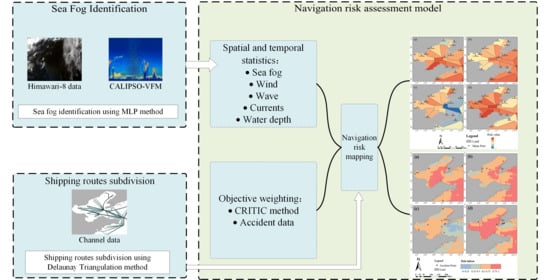
In order to evaluate the navigation risk in Bohai Sea and its surrounding waters, first, a sample database based on AHI data and CALIPSO vertical feature mask (CALIPSO-VFM) data is established, and a sea fog identification method based on Multilayer Perceptron (MLP) method is developed. Second, the method is used to obtain a large historical sea fog data set of the study area, which is combined with other evaluation factors to calculate the occurrence frequency of severe sea conditions. Then, the criteria importance through intercriteria correlation (CRITIC) objective weighting method is used to determine the weights of the evaluation criteria, and obtain navigation risk maps of the area via global information system (GIS) mapping technology. In order to further analyze the risks, the Delaunay triangulation method is used to divide the sea area into different waterway regions, and the risk values for the specific waterway areas are calculated. Finally, two validation methods are used to validate the sea fog identification method and navigation risk estimation model, and a sensitivity analysis of the model is carried out. A method flow chart of this process is shown in Figure 2.

3.1. Sea Fog Identification

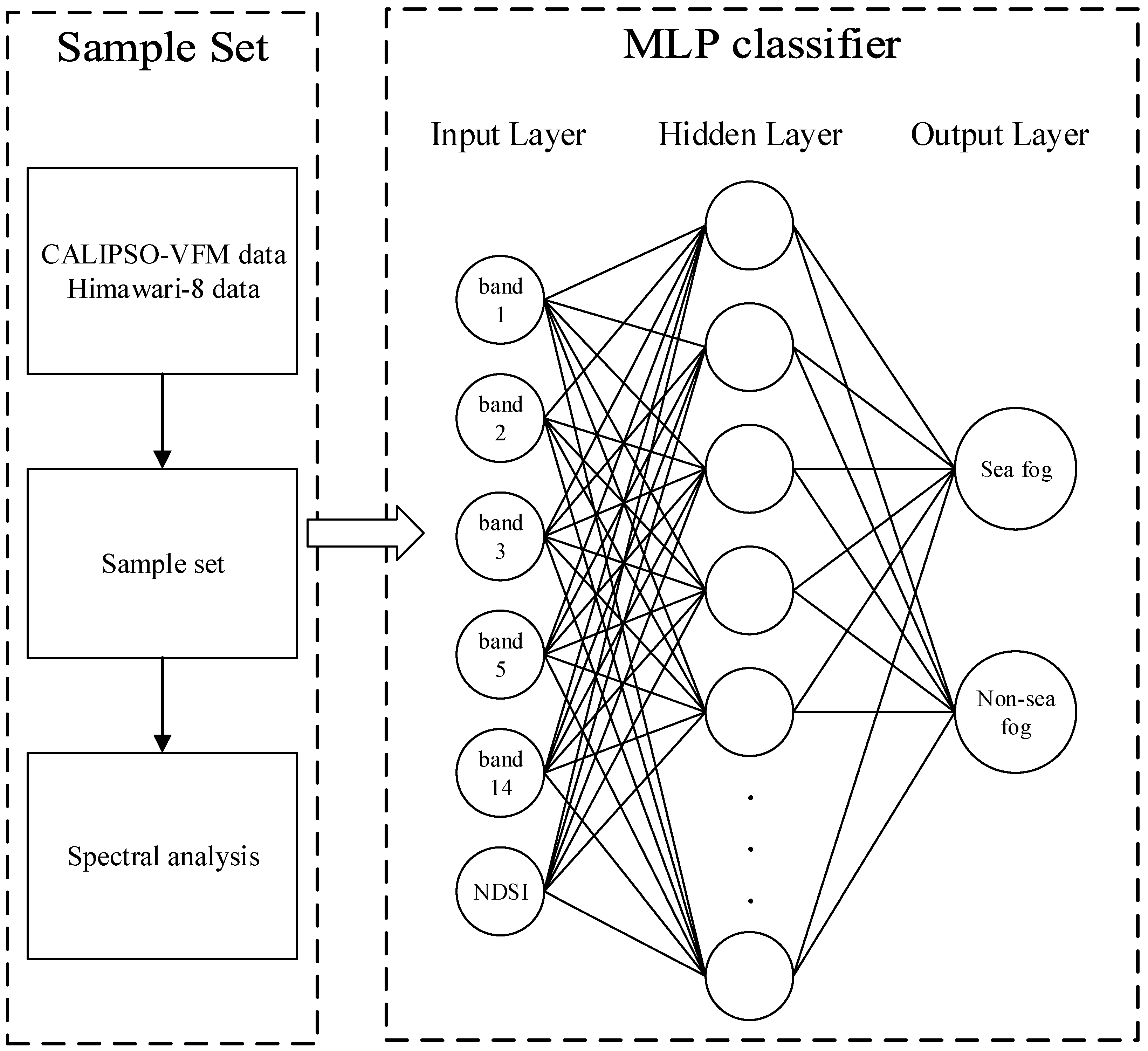
In this paper, the MLP method is used to identify sea fog in the study area. First, sea fog sample points are selected from the CALIPSO-VFM and AHI data sets. Then, the spectral characteristics and fusion spectra of sea fog and non-sea-fog samples are analyzed to select features that benefit the classification. After that, sea fog and non-sea-fog binary classification models are constructed by the MLP method, and the optimal parameters are selected through training experiments. The specific processes are shown in Figure 3.

3.1.1. Sample Selection of Sea Fog

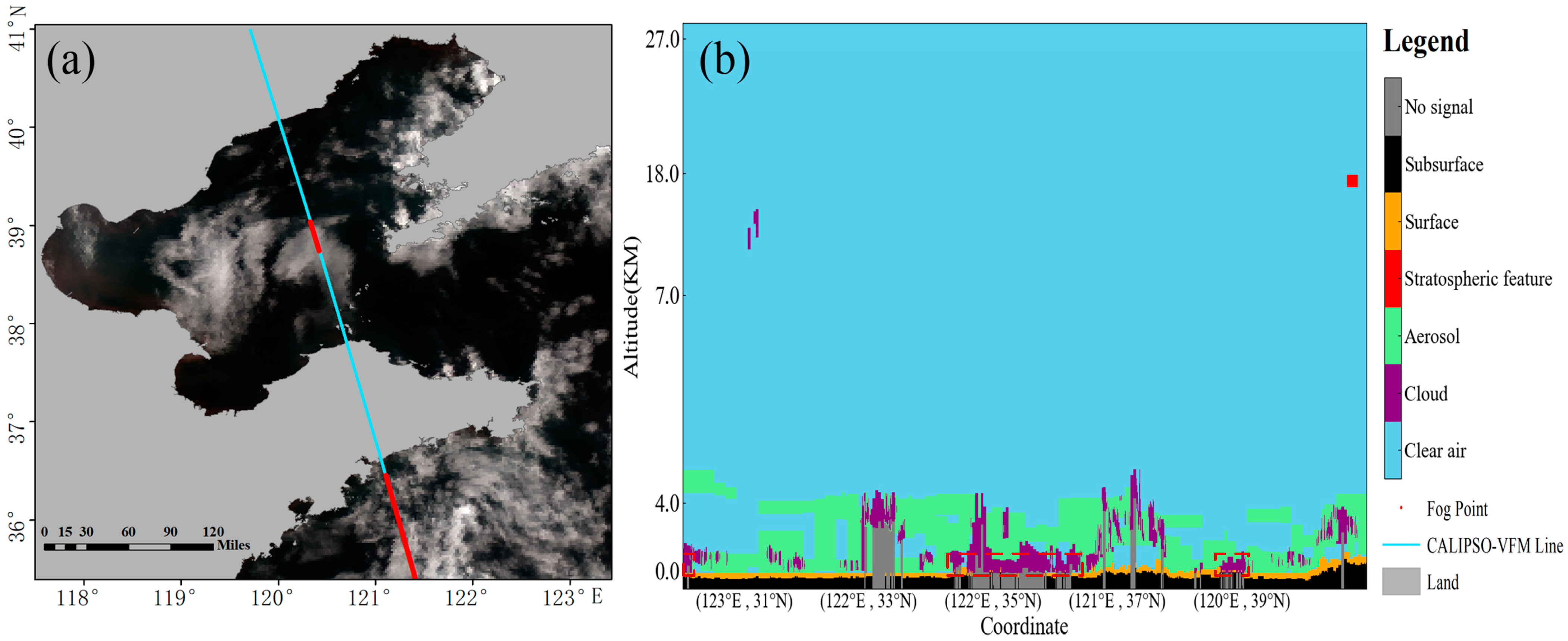
It is difficult to distinguish between sea fog and low clouds and stratus clouds through visual interpretations [32]. Therefore, a sea fog sample database is established using CALIPSO-VFM data to assist the selection of sea fog samples from AHI images [5,33]. Figure 4 shows the selection method, where Figure 4a is an AHI image on 15 June 2018 at 05:10 UTC, and Figure 4b is the classification result when using CALIPSO-VFM data from 15 June 2018 at 05:17 UTC. In the area in the red box in Figure 4b, the CALIPSO-VFM data are used to identify places where clouds are in contact with the sea surface, which are considered as sea fog points. From these, we extract the spectral values from the corresponding positions in the AHI images (e.g., the red dots in Figure 4a). Then, the spectral values at the sea surface, low clouds, and medium-high level clouds are obtained using the same approach. A total of 9141 samples of sea fog, 10,071 samples of the sea surface, 8733 samples of low clouds, and 10,771 samples of middle-high level clouds were selected and used in this paper.

3.1.2. Feature Selection

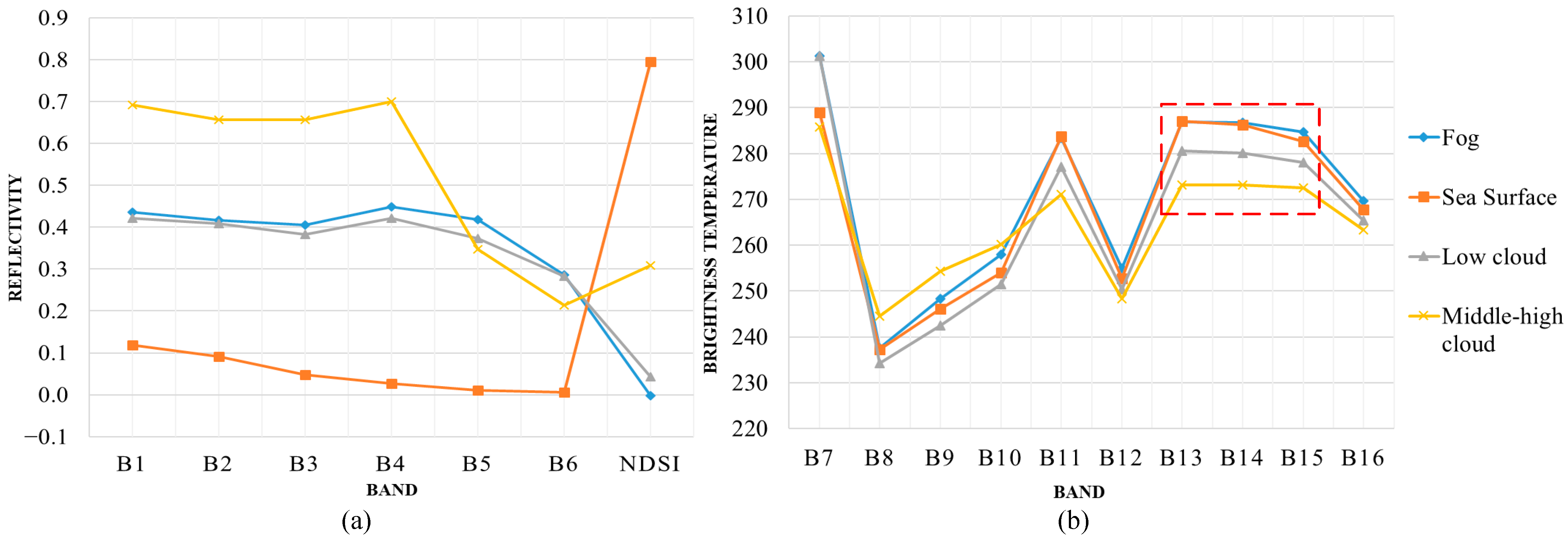
After obtaining the spectral features of each object, it is necessary to analyze the spectra to select features with better classification effect. The visible band of the Advanced Himawari Imager sensor onboard Himawari-8 consists of channels 1–3 (central wavelengths of 0.47 μm, 0.51 μm, and 0.64 μm, respectively); channels 4–6 are near-infrared bands (central wavelengths of 0.86 μm, 1.6 μm, and 2.3 μm, respectively), and channels 7–16 are infrared and far-infrared bands (central wavelengths of 3.9 μm, 6.2 μm, 6.9 μm, 7.3 μm, 8.6 μm, 9.6 μm, 10.4 μm, 11.2 μm, 12.4 μm, and 13.3 μm, respectively). The visible and near-infrared spectral characteristic curves of different objects are shown in Figure 5a. In the first three bands, the mid-high level clouds and the sea surface are significantly different from the sea fog and low clouds, but it is difficult to distinguish between low clouds and sea fog. With an increase of wavelength, the reflectance of all kinds of features gradually decrease, but the rate of change of sea fog in band 5 is significantly slower than that of other features, and the difference between the sea fog and the low clouds becomes obvious. According to [34], there are a large number of water droplets of 1 μm diameter in sea fog, which increase the reflectance measured in bands 4 and 5 and slow down the rate of change of reflectance in band 5; such behavior provides an obvious means to distinguish sea fog from other objects.
To identify more features, NDSI [11] is constructed with data from bands 2 and 5 (i.e., 0.51 μm and 1.6 μm), calculated using Equation (1) as:
NDSI = B 0.51 μ m B 1.6 μ m B 0.51 μ m + B 1.6 μ m ,
where B 0.51 μ m and B 1.6 μ m represent bands with central wavelengths of 0.51 μm and 1.6 μm, respectively, in the AHI data. It can be seen from Figure 5a that NDSI provides a significant distinction between sea fog and low clouds. There are also distinct intervals between different objects.
Figure 5b shows the characteristic curves of the different infrared bands. The brightness temperatures of sea fog and the sea surface are very similar, and cannot be used to effectively distinguish between them, even though the average height of low clouds is higher than that of sea fog, and the brightness temperature of the former is slightly lower. The brightness temperatures of middle-high clouds are the lowest, and this difference is more obvious in bands 13, 14, and 15 (see, e.g., the red dotted box in Figure 5b). Therefore, these three bands can be selected to further distinguish low clouds and sea fog.
Based on the spectral analysis, we selected bands 1, 2, 3, 5, and 14 and NDSI as classification features to construct the sea fog sample set.

3.1.3. Sea Fog Recognition Method Based on MLP

As a mature classification method, Multilayer Perceptron (MLP) method has been applied to various remote sensing image classification tasks [35,36]. In this paper, sea fog identification is taken as a binary-classification task to train the MLP classifier. The low clouds, sea surface, and medium-high level clouds are unified into a non-sea-fog category. The objective function of the MLP binary classification method can be described as shown in Equation (2) [37]:
min w , b 1 2 | | h w , b ( f ( w x + b ) ) y | | 2 ,
where w and b represent the weight and bias of each layers, y represents the sample labels, x represents the sample values, h w , b represents the output of the output layer, and f represents the activation function. The kernel objective in this paper is the sigmoid function, which can be described as given in Equation (3):
f ( x ) = 1 1 + exp ( x )   ,
Through training the MLP classifier, each parameter of the layers is obtained. The main training process consists of four steps:
  • Step 1: Normalize the sample values, which are scaled between [0, 1];
  • Step 2: Divide the training set and testing set, and train the MLP classifier using the former;
  • Step 3: Cross validation to determine the optimal parameters; and
  • Step 4: Complete MLP training and verify the accuracy of the classifier.
The partition ratio of training set to test set is 7:3, and the hidden layer sizes in this study is 100 × 100 , and the random state is 10, the optimizer solver is “adam”. Through training, a sea fog identification model based on AHI data is obtained, which is used to obtain a large amount of historical sea fog information in the research area. The verification method and accuracy results of sea fog identification are described in Section 3.3.1 and Section 4.1.

3.2. Navigation Risk Assessment Model

After creating a suitable sea fog data source, the navigation risk assessment model can be constructed according to various environmental elements in the study area. This section mainly includes four parts: first, the accident data are statistically analyzed to select the environmental factors that have the greatest impact on the navigation of ships in the study area. Second, the data of each evaluation factor are preprocessed. Third, we introduce a detailed process of determining the weights of each evaluation factor by the CRITIC objective weighting method, and then construct the navigation risk assessment model. Finally, we use the Delaunay triangulation method to divide the sea area into different navigational regions, and calculate the navigation risks in the specific navigational areas for further risk analysis.

3.2.1. Criteria for Navigation Risk

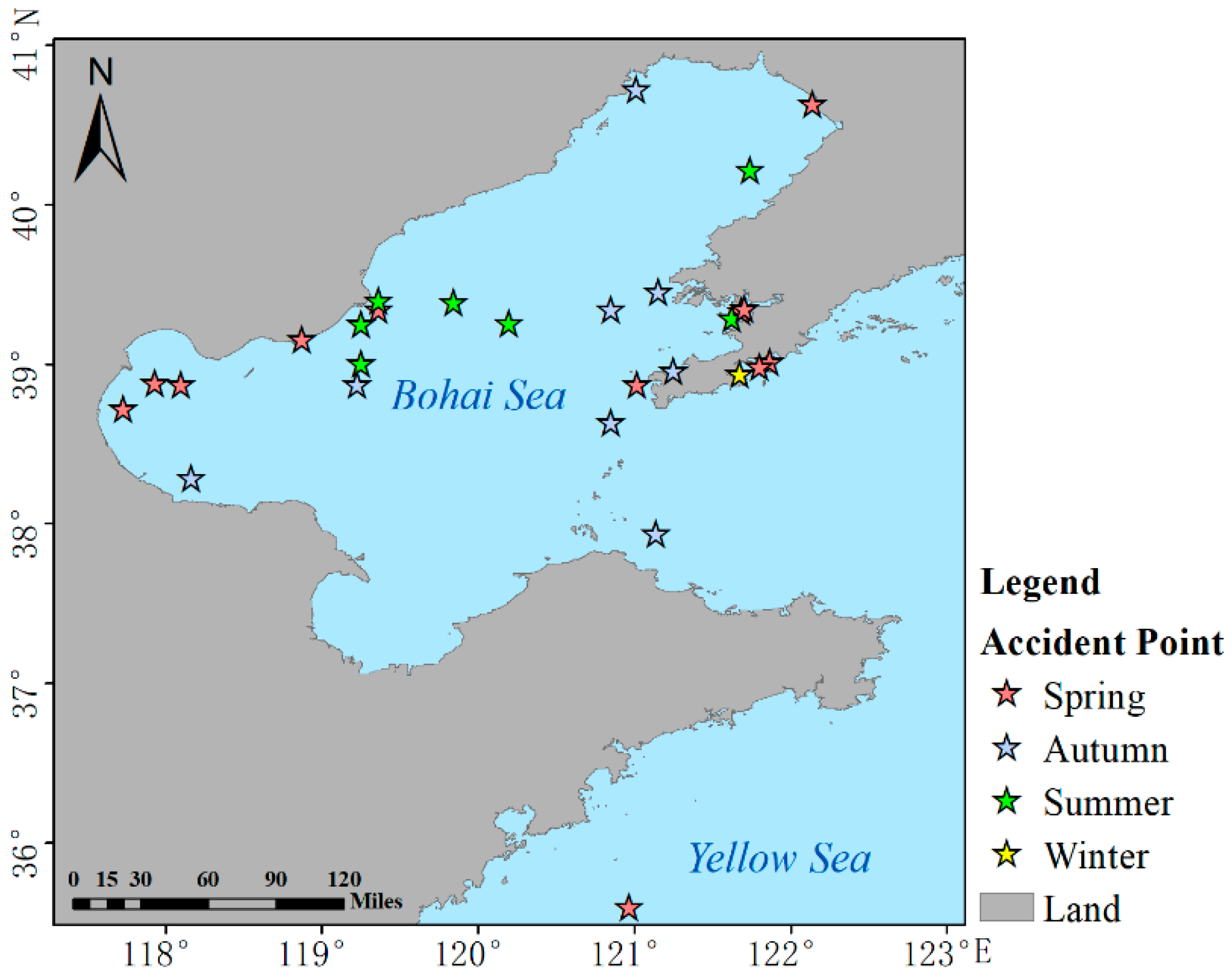
The identification of relevant criteria is a very critical step in the construction of an assessment model. The navigation risks mentioned in this paper refer to the loss of people or property and the possible impact of the navigation environment, which may consist of harsh conditions, resulting in the improper operation of the ship in the course of navigation, and which may cause ship collisions (i.e., the collision of two or more ships), collisions with stationary objects (i.e., with a reef, coast, or building), grounding (where the bottom of the ship touches the bottom of the sea due to insufficient water depth), or a sunken ship (sinking of ship) [38]. In order to obtain the criteria that may lead to identifying navigation risks more objectively, we use accident data from Maritime Safety Administration of the People’s Republic of China in study areas to determine criteria that have a greater impact on ship navigation. In this paper, environmental risks are mainly used for assessment, so the accidents caused by purely human factors need to be eliminated. After screening, a total of 39 accident records were included. The distribution of accident data is shown in Figure 6, where different color points represent accidents in different seasons.
The accident assessment section of each accident report details the main and secondary causes of the accident. As such, we used the accident assessment report to count the number of accidents caused by the different assessment factors. When selecting accident records, certain rules should be observed. For example, if there is a sentence whose meaning is similar to “heavy fog in the sea, poor visibility, crew neglected to look out, resulting in ship collision” in the accident cause assessment, it is considered that the accident is related to sea fog and “1” is added to the number of accidents caused by sea fog in the statistics. If there is a sentence whose meaning is similar to “the waters of the accident were affected by strong winds, and the ship failed to evacuate the sea in time, resulting in the collision of the ship”, it is considered that strong winds had an impact on the accident, and we added “1” to the number of accidents caused by strong winds to the statistics. When the accident is caused by a combination of various factors, such as “due to the superposition of strong wind, cold air, and storm surge in the accident water area” recorded in the report, it is considered that strong winds and big waves had an impact on the accident, and “1” is added to the statistics of each category. The statistical results of the final criteria involved in the historical accidents are shown in Table 2.
Finally, according to the statistical information and data support, the top five criteria were selected, which were waves, wind, sea fog, ocean currents, and water depth. These five criteria are meteorological and hydrological factors which are especially relevant in meteorological navigation. Specifically, gale weather has an impact on both sailing and berthing ships. Sailing ships are affected by gales when sailing, which will reduce the controllability of the ships. If berthed ships are not fully anchored, the hull may shift under greater wind pressure, resulting in grounding or a collision. When big waves occur, they are usually accompanied by strong winds. It is difficult for ships to adapt to the peaks and troughs of sea waves, and when ships with lower tonnages are hit by big waves, their external structure will be subjected to greater external forces, which may cause damage to the ship, which is very dangerous during navigation. Currents will also affect ship navigation. In narrow sea areas, the speed and direction of ocean currents are unstable, which makes it more difficult to effectively use seamanship. When sailing against the currents, the energy consumption of a ship increases, and the difficulty of navigation also increases [39].
Sea fog is the main reason affecting the visibility at sea. Many ship collisions, as well as touching and grounding accidents, are caused by sea fog. Generally, ships will avoid sailing in fog. However, when sea fog arises, it may be difficult for sailing ships to leave the fog area promptly. When sea fog occurs, the sea waves are generally small but limited by the field of vision. It is difficult for the crew to fully observe the surrounding navigation environment, and the probability of accidents increases greatly [40]. Water depth is a factor that must also be considered when planning passage through a channel. Before sailing, the captain should plan the route reasonably according to the ship’s draught and abundant water depth. Generally speaking, the nearshore sea is shallow, so when nearshore navigation is affected by other factors, grounding and collisions may easily occur. In addition, the water depth is related to sediment in the sea area, which may cause a change of water depth due to the movement of the sea water. If the relevant properties of the navigation area are not known in advance, accidents can easily occur.
In general, the five kinds of navigation environment criteria identified by the accident data statistics have a great impact on ship navigation, and are also the five main environmental factors about which the maritime industry are very concerned. At present, wind, waves, currents, and terrain factors can be supported by the existing product level data, but it is still difficult to obtain sea fog data in large areas. Therefore, this paper uses a remote sensing identification method to obtain the daily sea fog occurrence in Bohai Sea and its surrounding waters over a five-year period, using the method described in Section 3.1.3.

3.2.2. Data Processing

Five evaluation factors with a great impact on ship navigation were selected in Section 3.2.1. However, before conducing the risk assessments, the risk factor value of each criterion should be obtained in each of the four seasons. First, the spatial resolution of the gridded data are unified to 0.125° × 0.125°. Second, the risk values of each factor under severe sea conditions are calculated from the gridded wind, wave, ocean currents, and sea fog data from 2016 to 2020. Then, the risk grid values of each factor are standardized. When setting the thresholds for the different evaluation criteria, we follow the methods employed in previous research [21,41].
First, the sea fog criterion calculates the occurrence frequency of sea fog in each grid in the different seasons following Equation (4):
F i j = f i , k d j ,
where F i j represents the occurrence frequency of sea fog in grid i in season j , f i , k represents the occurrence of sea fog in grid i on day k ,   f i , k [ 0 ,   1 ] , 0 represents no sea fog, 1 represents sea fog, and   d j represents the total number of days in season   j .
The wind criterion, for wind speeds greater than 11.7 m/s in each grid, in different seasons is calculated via Equation (5):
G i j = g i , k d j ,
where G i j represents the frequency of wind speeds greater than 11.7 m/s in grid i in season j , g i , k represents wind conditions for grid i on day k ,   g i , k [ 0 ,   1 ] , 0 represents wind speeds slower than 11.7 m/s, 1 represents winds speeds greater or equal to 11.7 m/s, and   d j represents total days in season   j .
Calculation of the wave and currents criteria are same as for the wind criterion, where the thresholds for the wave and currents criteria are 2 m and 1 m/s, respectively.
The water depth is a static criterion, where each grid risk value of water depth is calculated using Equation (6):
D i = { 0                 d i > 30   m 1 d i 30       0   m < d i < 30   m 1                   d i < 0   m ,
where D i represents the risk value of water depth in grid i, and d i represents the original water depth value.
After calculating these criteria, it is necessary to standardize the grid values to 0–1. The standardization formula used in this paper is shown in Equation (7):
x = x x min x max x min ,
where   x represents the standardized value, x represents the original risk value, x min represents the minimum value, and x max represents the maximum value.

3.2.3. Weighting the Criteria Using CRITIC

Weights can reflect the importance of each evaluation criterion, and the method of weighting is an important step in building a spatial, multi-objective decision model. The traditional way to obtain weighting data is from an expert’s knowledge or a questionnaire, which inevitably involve some subjective uncertainties. With the aim of eliminating subjectivity as much as possible, we collected accident data from 2015 to 2021 in Bohai Sea and Yellow Sea, and reproduced the values of each evaluation factor during the accident using the CRITIC weighting method to get the criteria weights. The CRITIC method determines weights according to the discretization of each criterion and the relationships between them [42], and is widely used in weight determination problems [43,44]. In this paper, the CRITIC method is used to get the criteria weights from historical accident data. The specific weight determination steps are as follows.
  • Step 1. The accident value of each criterion is standardized using Equation (7).
  • Step 2. The standardized data are organized into an evaluation matrix. The columns represent different criteria, and the rows represent the standardized value of the same criteria, as shown in Equation (8):
    [ x 11 x 12 x 21 x 22 x 1 k x 2 k x n 1 x n 2 x n k ] ,
    where k represents the total number of criteria, n represents the total number of accident records, and x represents the standardized value.
  • Step 3. Calculate the correlation coefficients, and a correlation coefficient matrix is obtained, expressed as Equation (9). Then, the conflict coefficient of each evaluation factor is calculated by Equation (10):
    [ r 11 r 12 r 21 r 22 r 1 k r 2 k r k 1 r k 2 r k k ] ,
    R z = m = 1 k ( 1 r z , m ) z [ 1 , , k ] ,
    where R z represents the conflict coefficient of criterion z , and r z , m represents the correlation coefficients between criteria z and m . Note that a bigger correlation between criterion z with other criteria produces a smaller R z .
  • Step 4. Calculate the sample standard deviation of each criterion using Equation (11):
    S z = l = 1 n ( x l x ¯ ) 2 n 1 ,
    where S z represents the sample standard deviation of criterion z , and x ¯ is the mean of the standardized values.
  • Step 5. The amount of information for criterion z is calculated with the conflict coefficient R z obtained in Step 3 via Equation (12):
    C z = S z · R z ,
    where C z represents the amount of information of criterion z .
  • Step 6. Normalize the amount of information and get the CRITIC weights for each criterion following Equation (13):
    w z c = C z m = 1 k C m ,
    where w z c represents the CRITIC weight of criterion z .
Through the above six steps, the CRITIC method can be used to obtain the different criteria weights. When the correlations between a criterion and other criteria are large and the variances are small, the CRITIC weight of this criterion will be relatively small. Thus, this method can make a tradeoff between the correlations and the standard deviations of the different factors, and hence give more reasonable weight values. The final weight of each criterion is combined with the accident statistics (see Table 2) using Equation (14):
w z = w z   c × Q z m = 1 k w m c × Q m ,
where w z represents the final weight of criterion z , and Q z represents the normalized statistics of criterion z , obtained from Table 2.
The correlation coefficients of the five criteria are shown in Table 3. The high correlation coefficient between the wind and wave criteria indicates a certain correlation between wind and waves in accidents. The weak negative correlation between sea fog and wind reflects that it is not easy to generate sea fog in gale weather. The correlations between ocean currents with the other factors are small reflecting that the ocean currents are less affected by other environmental factors. The weighting results are shown in Table 4 in descending order: sea fog, waves, wind, depth, and currents.
The navigational risk value is calculated through Equation (15):
R i = z = 1 k w z × x i , z ,
where R i represents the navigational risk value in grid i, and x i , z represents the standardized value of criterion z in grid i. The calculated navigational risk values are standardized using Equation (7). After standardization, the final navigational risk assessment values are obtained, which are divided into four levels: [0, 0.25), [0.25, 0.5), [0.5, 0.75), and [0.75, 1], representing “safe”, “a little safer”, “a little dangerous”, and “dangerous”, respectively.

3.2.4. Shipping Routes Subdivision

To provide a suitable risk analysis of specific shipping lanes in Bohai Sea and its surrounding waters, 107 main shipping routes officially recommended by the China Maritime Safety Administration in the study area [31] are considered in this paper (as shown in Figure 7). Next, the shipping routes are manually simplified (as shown in Figure 8a). Then, the Delaunay triangulation method is used to divide the navigation area into the main shipping routes. The main steps of this process are described as follows.
  • Step 1: Merge and simplify the dense shipping routes;
  • Step 2: Generate equally spaced route points along the simplified shipping routes;
  • Step 3: Use the Delaunay triangulation method to generate a regional Tyson polygon network with route points as the source;
  • Step 4: Merge polygons from the same source to form a route subdivision;
  • Step 5: Trim the boundaries manually.
A subdivided region is obtained after trimming, where the sea area is divided into different regions according to the shipping routes, as shown in Figure 8a–c. The black line segments in Figure 8a show the simplified shipping routes, and the green points are the route points generated at equal intervals along the routes. Figure 8b shows the Tyson polygon network generated by the route points, and Figure 8c shows the regional channel network after merging and trimming.
By dividing the sea areas into different routes, a risk analysis can be clearly conducted on each specific route area. The mean risk value represents each route’s region risk for every area, which is calculated as Equation (16):
R d ¯ = R s u m d A d ,
where R d ¯ represents the risk value of region d, R s u m d represents the total risk value of region d, and A d represents the area of region d. By classifying the risks in each region of each route, the risks therein can be further analyzed. Section 4.4 describes the analysis results.

3.3. Validation Methods

3.3.1. Sea Fog Identification Validation Using the CALIPSO-VFM Points

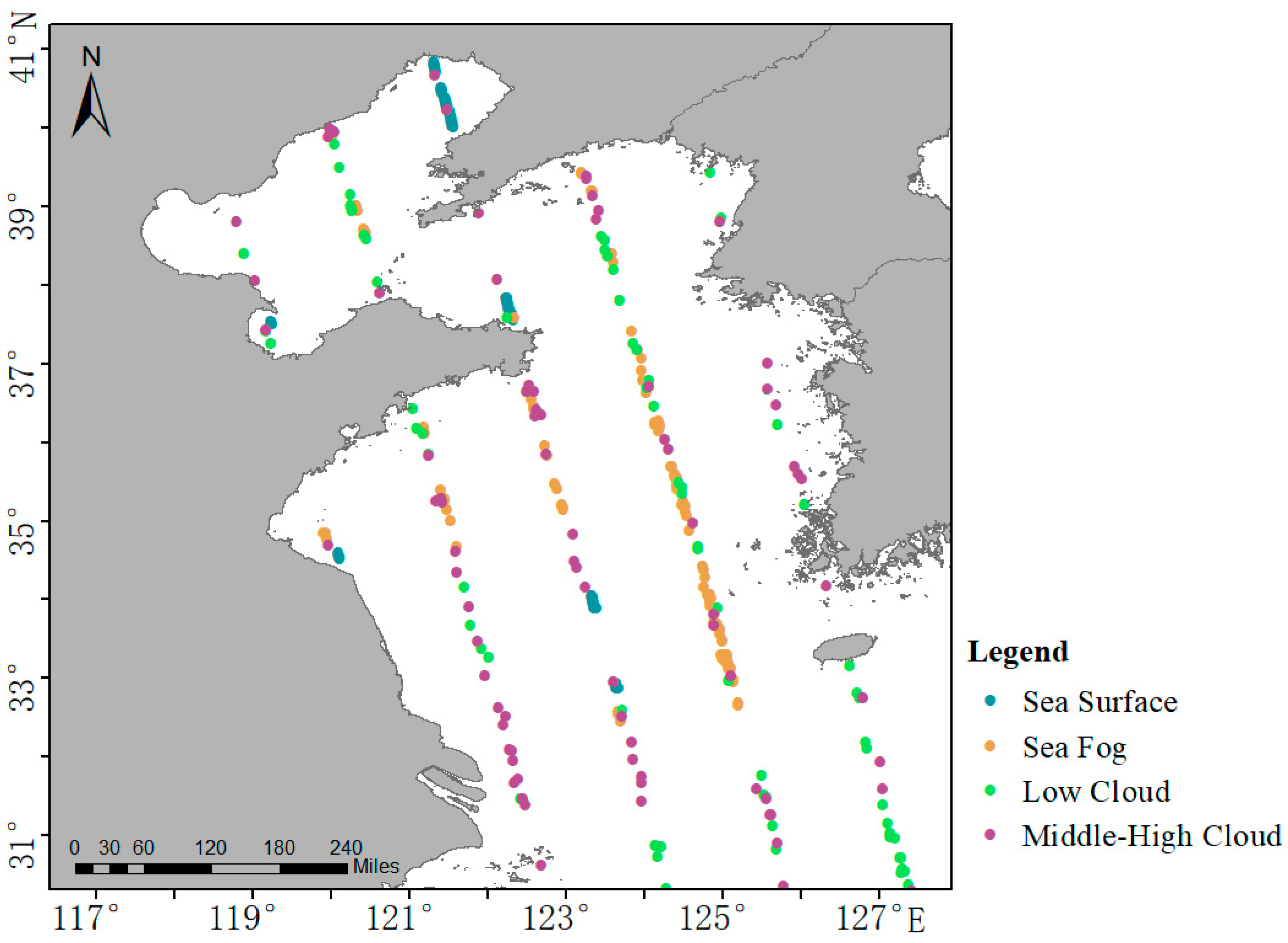
In this paper, CALIPSO-VFM data are used for sea fog verification. The CALIPSO-VFM data of Bohai Sea and Yellow Sea from January to September in 2018 are selected to identify different types of ground objects along the trajectory lines, which are treated as different object points. The observing times of the AHI data and CALIPSO-VFM data are controlled within 10 min. After obtaining the sea fog inversion results using the MLP method, the confusion matrix is counted, and the spatial distributions of the track points are obtained, as shown in Figure 9. Four types of ground objects are clearly indicated here, but only sea fog and non-sea-fog are required for the analysis made in this paper. The detailed classification made here allows us to further analyze the algorithm’s accuracy. This paper compares and analyzes the results obtained with the proposed MLP method with those obtained by the NDSI threshold method proposed by [11], and the specific results are shown in Section 4.1.1.

3.3.2. Navigation Risk Evaluation Validation Using the Accident Points

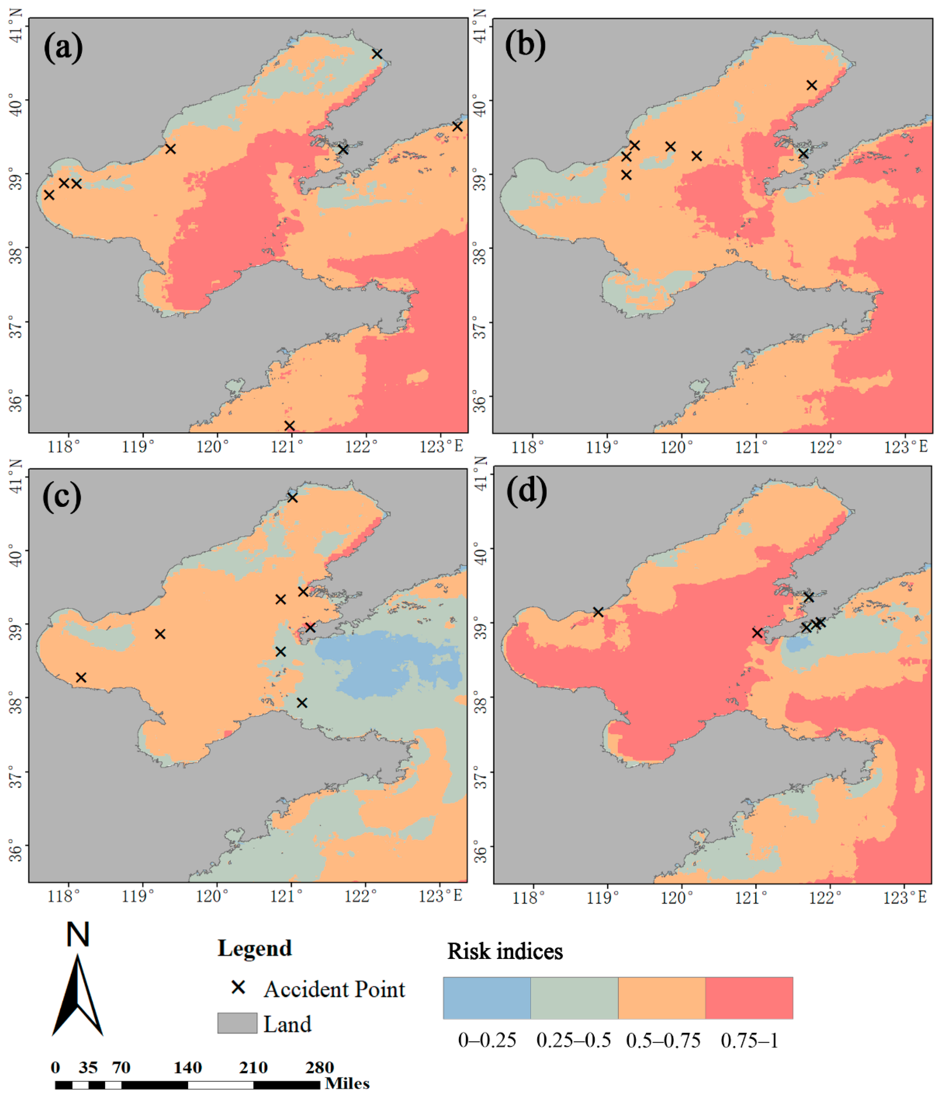
This paper uses accident data to verify the accuracy of the evaluation model. The collected accident reports are treated as accident points, which are divided into four subsamples based on the four seasons (e.g., spring, summer, autumn, and winter). The specific distribution of the accident points is shown in Figure 6. When matching the accident points with the navigation risk evaluation results in the same season, if an accident point occurs in a high-risk area (i.e., a risk value greater than or equal to 0.5), the match is successful; if it occurs in a low-risk area (i.e., a risk value less than 0.5), the match is not successful. The matching degree of the model with the accidents was verified by counting the matching rate, and the results are shown in Section 4.2.

3.3.3. Sensitivity Analysis

A sensitivity analysis can be used to analyze the stability of a model and observe the stability of the evaluation criteria weights. The one-at-a-time method is a widely used sensitivity analysis method for spatial multi-objective decision technology [45,46], where the sensitivity increase/decrease of the spatial evaluation results is calculated by way of the aggregate mean, which has been applied to the risk evaluation model in this paper.
The main steps of the method are as follows. First, for criteria a , the weight value is increased and decreased using 10% equal intervals. The scaling range is [−50%, 50%], and the new weight of criteria a is obtained using Equation (17):
w a ¯ ( c r ) = ( 1 + c r ) * w a   ,
where w a ¯ ( c r ) represents the new weight of criteria a , c r is the increased/decreased value, and w a represents the original weight. To ensure that the summed weights equal 1, Equation (18) is calculated for the remaining criteria:
w ¯ h ( c r ) = w h × 1 w a ¯ 1 w a ,
where w ¯ h ( c r ) represents the weights adjusted for the remaining criteria, ( h a ) , and w h represents the original weight of criterion h .
Then, the new risk evaluation values are calculated using the adjusted weights, as shown in Equation (19):
R ( w a , c r ) = w a ¯ × x a + a h n w h ¯ × x h ,
where R ( w a , c r ) represents the new risk evaluation value for each grid, x a represents the standardized value of criterion a for each grid, and x h represents the standardized value of criterion h for each grid.
The mean of the absolute change rate (MACR) of the whole region is calculated to obtain the change rate of criterion a with changes c r , following Equation (20):
MACR ( w a , c r ) = j = 1 S 1 S | R j ( w a , cr ) R j 0 R j 0 | × 100 % ,
where MACR ( w a , c r ) represents the MACR of the risk evaluation in the whole region,   R j ( w a , cr ) represents the risk evaluation value of the j-th grid after weight adjustment, and R j 0 represents the original risk evaluation value, S represents the total number of grids.
If the adjustment amplitude of a criterion weight is far less than the change amplitude of the model result, it indicates that the proposed model has good stability. The results of the sensitivity analysis are shown in Section 4.3.

4. Results

4.1. Sea Fog Identification

4.1.1. Identification Precision

The MLP sea fog identification method was applied using Python programming, and the algorithm was verified using the CALIPSO-VFM classification points; the results it produced were then compared with those obtained with the NDSI threshold method proposed by [11]. The accuracy evaluation indices used in this paper are based on the work of [7], including the probability of detection (POD), probability of false detection (PFD), probability of missing detection (PMD), and equitable threat score (ETS). The calculation formulas of the four indicators are respectively shown in Equations (21)–(24):
POD = H H + M ,
PFD = F F + C ,
PMD = M H + M ,
ETS = H ( H + F ) ( H + M ) / N H + M + F ( H + F ) ( H + M ) / N
where H represents the number of verification data points related to sea fog, C represents the number of verification data points that are all non-sea fog related, F represents the number of non-sea-fog data points that the algorithm incorrectly identifies as sea fog, and M represents that the verification data that are sea fog, but the algorithm incorrectly identifies as non-sea-fog. N represents the total number of points.
The confusion matrix of the results from the two algorithms (i.e., the MLP sea fog identification algorithm and NDSI threshold method) is shown in Table 5, and the precision comparison results are shown in Table 6.
It can be seen from the results that the POD of both MLP sea fog identification algorithm and NDSI threshold method are more than 80%; indeed, the NDSI threshold algorithm identifies eight more sea fog points relative to the MLP method. However, the NDSI threshold algorithm identifies more non-sea-fog points as sea fog, resulting in lower accuracy indices tested by the algorithm. These non-sea-fog points are mainly low clouds, indicating that the NDSI threshold algorithm is not able to effectively distinguish between sea fog and low clouds. The MLP sea fog classification method is relatively stable for the various accuracy indices. Although the POD value of the MLP method is smaller than that of the NDSI threshold algorithm, the former algorithm is more able to distinguish between sea fog and non-sea fog points than the NDSI threshold algorithm, with an ETS of 59.22%. Therefore, the MLP sea fog classification method constructed in this paper performs better than the NDSI threshold algorithm on the whole.

4.1.2. Sea Fog Statistics

We applied the constructed sea fog identification algorithm to AHI data to get the sea fog information of 1442 days in the study area from 2016 to 2019, and calculated the sea fog occurrence of each grid in the four seasons. The location of Bohai Sea is about 37° N, and according to the climate of the region, we set February to April as spring, May to July as summer, August to October as autumn, and November to January of the next year as winter. Following these classifications, the fog occurrence of the four seasons in the study area is shown in Figure 10.
The sea fog in the study areas begins from the winter, and goes until the next autumn. The occurrence frequencies of sea fog in spring and summer are higher, while those in autumn and winter are lower; thus, the seasonal occurrence of sea fog shows obvious differences. From winter to the next autumn, the high incidence area of sea fog shows a trend of developing from south to north, and from west to north.
From the perspective of spatial distribution, in winter, the higher frequency areas of sea fog are in the west of Bohai Sea, and with an eastward movement tendency with time. In spring, higher frequency areas of sea fog are in the Yellow Sea and south of Bohai Sea, with a northward movement tendency with time. The two tendencies gather in the south of Bohai Bay in summer, when the frequency of sea fog reaches its highest value in the whole year.
On the other side, the frequency of sea fog in spring and summer is greater than that in autumn and winter, and in winter, strong winds are frequent, which have a greater impact on navigation than sea fog [25]. Therefore, this paper considers the spring and summer as the main fog seasons (February to July). This result will be useful for navigational risk analyses.

4.2. Navigation Risk Evaluation Validation

The navigation risk evaluation model was coded in the R language and ArcGIS software. The matching results between the evaluation results and accident points are shown in Figure 11a–d, the latter of which respectively shows the results from in spring, summer, autumn, and winter. The specific matching results are shown in Table 7.
The matching degree of the navigation risk evaluation model is 69.9%. In summer, the matching degree reaches 85%, where only one accident point is not successfully matched. In winter, the matching rate is low, only 33%, and four accident points are not successfully matched. Of the four unsuccessfully matched accident points in winter, three are concentrated on the eastern side of Bohai Sea, and occur around a similar time (within three days) and in a similar area. The concentrated accidents have high randomness, leading to a low matching degree in winter. Except for winter, the matching degrees of accidents in the other three seasons are good, where only 1–2 points are not matched successfully. In the fog season (spring and summer), the matching degree of the proposed model reaches 80%; thus, the evaluation performance is great in the fog season.
It should be noted that the small amount of accident information is distributed randomly in space and time. The overall matching degree of the model is 69.9%, and the matching degree during the fog season is 80%. It can be considered that the model has a good matching ability to accidents in the case of limited accident data, especially for fog seasons.

4.3. Sensitivity Analysis

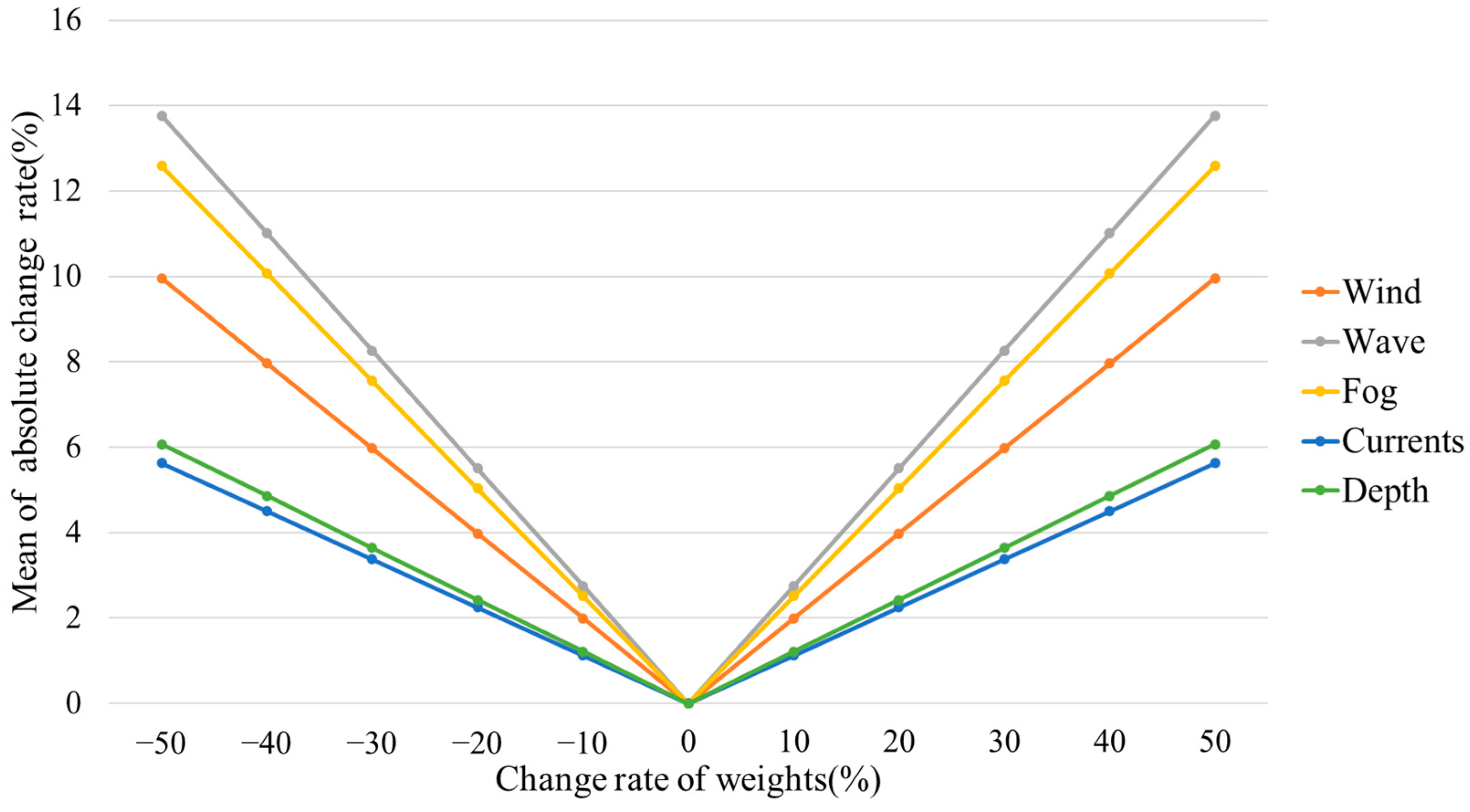
A sensitivity analysis can be used to analyze the fitting degree between model weights and criteria values. Figure 12 shows the sensitivity analysis results of the one-to-a-time method.
It can be seen from the results that the most sensitive criterion is waves, and the least sensitive criteria are currents. The descending order of sensitivity is waves, sea fog, wind, water depth, and currents. The maximum change rate is 14% when the change amplitudes of the criteria weights reach a maximum of 50%, and the corresponding change ratio is 0.28. The change rates of the evaluation results are much smaller than those of the criteria weights, which means the weights obtained by the CRITIC objective weight method are in good agreement with the criteria values, and the proposed navigation risk evaluation model has good stability.

4.4. Navigation Risk Analysis

According to the results of the navigation risk assessment in the four seasons given in Figure 11, winter has the greatest navigation risk in the study area throughout the year. In winter, accompanied by large winds and waves, sea fog weather also occurs occasionally, and the navigation risk in the sea area is high. The descending order of risk levels in the other seasons is spring, summer, and autumn.
In winter, the navigation risk in the southern part of the study area is greater than in the northern part. In spring, the high-risk navigation area is concentrated in the central part of Bohai Sea, extending from south to north. The high-risk area in spring has a trend of developing to the outer side of Bohai Sea. In summer, the high-navigation risk area retreats to outside of the Bohai Strait, and the risk value in the northern Yellow Sea increases. In autumn, the risk value in the sea area decreases to a minimum, although the western part of Bohai Sea has a relatively high value.
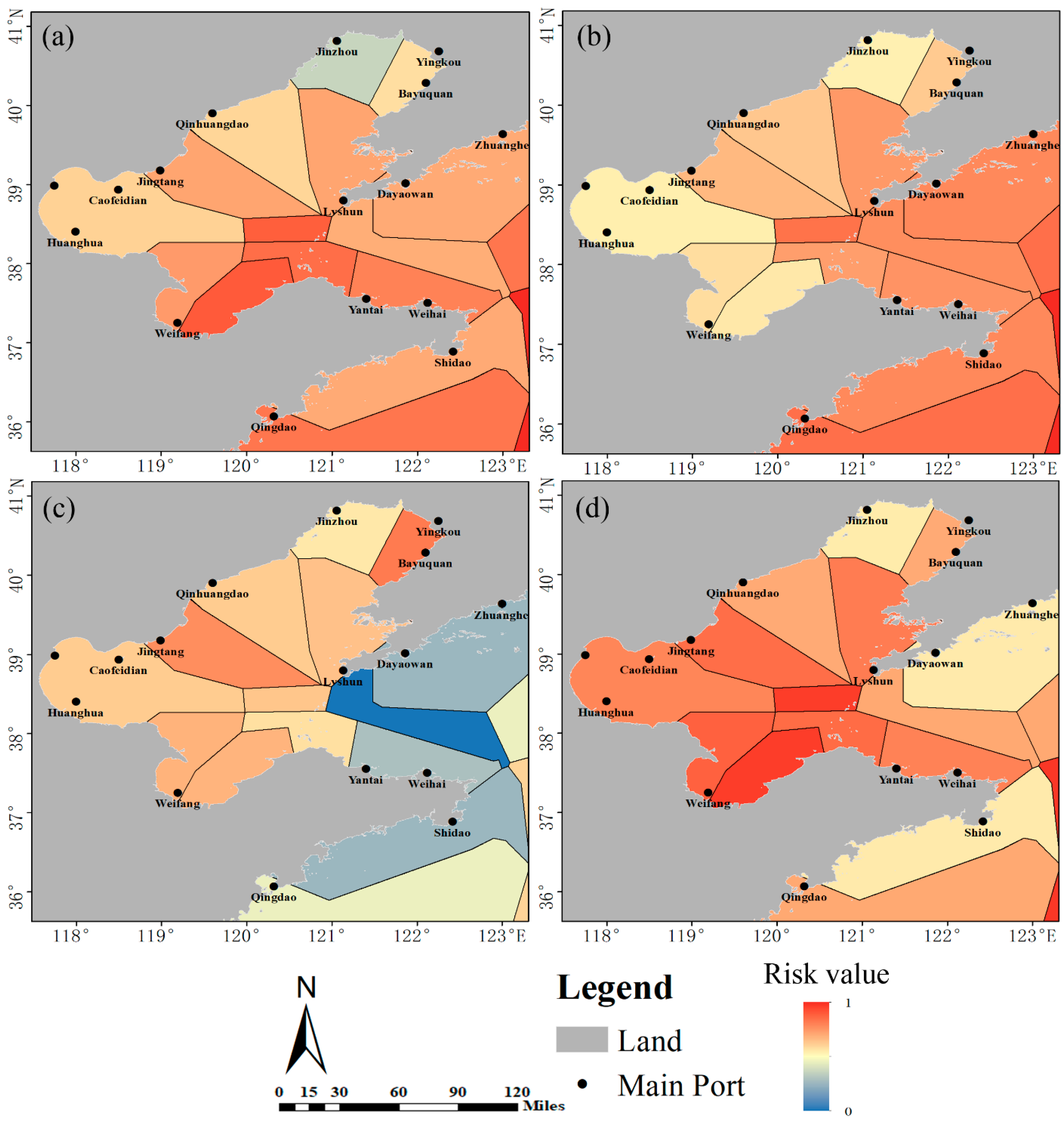
For further analysis, the evaluation results were calculated for every shipping region, as shown in Figure 13. In winter and spring, high-risk shipping regions are in the south, where the risks are high on the routes to Laizhou Port, Yantai Port, Harbor Port, Shidao Port, and Qingdao Port. In summer and autumn, high-risk shipping regions are in the north, and the risks are higher on the routes to Yinkou Port, Dalian Port, and Dandong Port. Other high-risk routes are from Qingdao Port to Yantai Port in spring and summer, and from Tianjin Port to Yantai Port and Shidao Port in spring and summer.

5. Discussion

In the navigation risk assessment framework proposed in this paper, we utilized a remote sensing sea fog identification method to obtain a large amount of accurate historical sea fog data in Bohai Sea and its surrounding waters. In the experiment, we found that the statistical results of sea fog are disturbed by low clouds, which could bring some abnormal statistic values (for instance, some areas with more than 200 days of sea fog in a year). In order to improve the classification accuracy, we used CALIPSO-FVM data to construct the sea fog sample set, and selected the features that contribute to the classification by spectral analysis. Compared with the NDSI threshold method in [11], the POD of proposed method decreased by 7.41%, but the ETS increased by 27.61%, which has a better distinguishing performance on sea fog and low clouds. It is very useful to have the historical frequency statistics of sea fog. The spatial distribution and seasonal differences of sea fog frequency in Bohai Sea and its surrounding waters are very obvious (Figure 10), the anomaly statistics disappear, and the results can be applied to the navigation risk assessment model. However, the proposed method still has some limitations. The small sample set size and unbalanced sample proportion are two factors that restrict the classification performance. The number of accurate sea fog samples obtained from CALIPSO-VFM data in Bohai Sea and Yellow Sea is limited, resulting in an unbalanced sample proportion (the sample ratio of sea fog to non-sea fog data is 1:3). It is necessary to expand the sample set size further. Observation data from weather ships or ground stations may be a viable option, which will be performed in a future study.
In order to eliminate the subjectivity in the navigation risk assessment methods, we collected the ship accident data of the study area for many years, and used the objective weighting method to determine the weight of criteria, from the accident matching and sensitivity analysis results, it has achieved a good performance in Bohai Sea and its surrounding waters. There are still some limitations that could be ameliorated further. Firstly, the spatial resolution and data performance of datasets used in this paper are quite different (for instance, the resolution of wind data is 0.25° × 0.25°, but the resolution of the currents is 0.125° × 0.125°). Some data need to be unified by interpolation, as it is expected that high-quality data could get the better risk-mapping results. Secondly, we significantly consider the navigation environment factors in the model, and some thresholds about ship factors follow the methods employed in previous research [21,41]. In the analysis about the ship, even the human factors could be added in the model and the applicability of the model will get a better performance.
In addition, with the development of geostationary orbit satellite and satellite constellation observation technology, ocean state observation data like wind, sea surface temperature, sea fog, etc. can be obtained in near real time. The historical or monitoring data of sea fog derived from Himawari-8 data have been integrated into a risk model of the proposed method; however, real-time sea fog observation data will be expected to be applied in risk assessment when the temporal resolution is further improved by satellite constellation. Using the real-time sea state observation data to evaluate and forecast navigation risks will greatly enhance the risk warning capability of the model, but it is a great challenge to develop a navigation risk forecast system. The dynamic Bayesian network could be a solution: for example, Paper [47] used dynamic Bayesian network to predict the risk of current and future time. Although this study only considers some risk factors of the ship itself and does not make use of the observed data of the space marine environment, it may be a feasible method for the prediction of navigation risk. Secondly, if the forecast data of the sea state (like wind, currents, etc.) could be obtained, the spatial multi- criteria decision-making method like this paper proposed can be used to evaluate risk on the basis of the forecast data, which will improve the spatial expression ability of the model. In general, the development of a spatial navigation risk prediction system is a great challenge, but it is worth performing it in future work.

6. Conclusions

This paper proposed a navigation risk evaluation method for Bohai Sea and its surrounding waters in the fog season. The MLP method was used to build a sea fog identification method, and with this method, a sample of sea fog historical information in the study area, obtained from AHI data, was obtained. The CRITIC method was used to weight the various criteria, which included sea fog, wind, waves, currents, and water depth. Then, a navigation risk evaluation was conducted using GIS mapping technology. For a better risk analysis of specific shipping lanes in the study area, the Delaunay triangulation method was used to divide the navigation area, and specific risk evaluation results of the navigation area were obtained. The POD of the sea fog identification method was 81.48%, the EST was 59.22%, and the accident matching rate of the navigation risk evaluation model was 80% in the fog season. The stability of the model was verified by a sensitivity analysis.
This study can provide a reference for ship navigation, ship route planning, and risk control in the four seasons in Bohai Sea and its surrounding waters. At the same time, the division of the waterway area can provide some planning advice for the various ports therein and the China Maritime Safety Administration, and may provide some help for maritime cargo transport and maritime rescue.

Author Contributions

Z.Z., P.D. conceived and designed the research, and performed the experiments. P.D., C.Q., L.J. wrote and edited the paper. J.Z., L.L., J.Y., S.L. analyzed the result and gave advice for the preparation and revision of the paper. Z.Z. and S.L. supervised the project. All authors have read and agreed to the published version of the manuscript.

Funding

This research was supported by the National Key R&D program 2017YFC1405600, and Natural Science Foundation of Shandong Province 2019GHY112034.

Institutional Review Board Statement

Not applicable.

Informed Consent Statement

Not applicable.

Data Availability Statement

The data used in this paper are all public data sets, which can be obtained free of charge through websites and books. The data sources are detailed in Table 2.

Acknowledgments

We thank the European Centre for Medium-Range Weather Forecasts, and Japan Aerospace Exploration Agency for Public available data. We thank the Maritime Safety Administration of the people’s Republic of China for public ship accident reports. Finally, thanks to the verification data support of sea fog by Xiaofei Guo, and anonymous reviewers for constructive and helpful suggestions on the manuscript.

Conflicts of Interest

The authors declare no conflict of interest.

References

  1. Xian, J.; Han, Y.; Huang, S.; Sun, D.; Zheng, J.; Han, F.; Zhou, A.; Yang, S.; Xu, W.; Song, Q.; et al. Novel Lidar algorithm for horizontal visibility measurement and sea fog monitoring. Opt. Express 2018, 26, 34853–34863. [Google Scholar] [CrossRef] [PubMed]
  2. Gao, Y.; Jiang, G. Research on Influencing Factors and Countermeasures of Fog Navigation in Weihai Harbour. In Proceedings of the 5th International Conference on Education, Management, Arts, Economics and Social Science, Sanya, China, 10–11 November 2018. [Google Scholar]
  3. Dorman, C.E.; Mejia, J.; Koračin, D.; McEvoy, D. World marine fog analysis based on 58-years of ship observations. Int. J. Clim. 2019, 40, 145–168. [Google Scholar] [CrossRef]
  4. Fu, G.; Guo, J.; Pendergrass, A.; Li, P. An analysis and modeling study of a sea fog event over the Yellow and Bohai Seas. J. Ocean Univ. China 2008, 7, 27–34. [Google Scholar] [CrossRef]
  5. Wu, D.; Lu, B.; Zhang, T.; Yan, F. A method of detecting sea fogs using CALIOP data and its application to improve MODIS-based sea fog detection. J. Quant. Spectrosc. Radiat. Transf. 2014, 153, 88–94. [Google Scholar] [CrossRef]
  6. Chunyang, Z.; Jianhua, W.; Shanwei, L.; Hui, S.; Yanfang, X. Sea fog detection using U-net deep learning model based on MODIS data. In Proceedings of the 2019 10th Workshop on Hyperspectral Imaging and Signal Processing: Evolution in Remote Sensing (WHISPERS), Amsterdam, The Netherlands, 24–26 September 2019. [Google Scholar]
  7. Shin, D.; Kim, J.-H. A New Application of Unsupervised Learning to Nighttime Sea Fog Detection. Asia Pac. J. Atmos. Sci. 2018, 54, 527–544. [Google Scholar] [CrossRef] [Green Version]
  8. Yang, J.-H.; Yoo, J.-M.; Choi, Y.-S. Advanced Dual-Satellite Method for Detection of Low Stratus and Fog near Japan at Dawn from FY-4A and Himawari-8. Remote Sens. 2021, 13, 1042. [Google Scholar] [CrossRef]
  9. Kim, D.; Park, M.-S.; Park, Y.-J.; Kim, W. Geostationary Ocean Color Imager (GOCI) Marine Fog Detection in Combination with Himawari-8 Based on the Decision Tree. Remote Sens. 2020, 12, 149. [Google Scholar] [CrossRef] [Green Version]
  10. Bessho, K.; Date, K.; Hayashi, M.; Ikeda, A.; Imai, T.; Inoue, H.; Kumagai, Y.; Miyakawa, T.; Murata, H.; Ohno, T.; et al. An Introduction to Himawari-8/9—Japan’s New-Generation Geostationary Meteorological Satellites. J. Meteorol. Soc. Jpn. Ser. II 2016, 94, 151–183. [Google Scholar] [CrossRef] [Green Version]
  11. Ryu, H.; Hong, S. Sea Fog Detection Based on Normalized Difference Snow Index Using Advanced Himawari Imager Observations. Remote Sens. 2020, 12, 1521. [Google Scholar] [CrossRef]
  12. Sahin, B.; Kum, S. Risk Assessment of Arctic Navigation by using Improved Fuzzy-AHP Approach. Int. J. Marit. Eng. 2015, 157, 241–250. [Google Scholar]
  13. Hu, S.; Fang, Q.; Xia, H.; Xi, Y. Formal safety assessment based on relative risks model in ship navigation. Reliab. Eng. Syst. Saf. 2007, 92, 369–377. [Google Scholar] [CrossRef]
  14. Balmat, J.-F.; Lafont, F.; Maifret, R.; Pessel, N. A decision-making system to maritime risk assessment. Ocean Eng. 2011, 38, 171–176. [Google Scholar] [CrossRef]
  15. Zhang, C.; Zhang, D.; Zhang, M.; Lang, X.; Mao, W. An integrated risk assessment model for safe Arctic navigation. Transp. Res. Part A Policy Pract. 2020, 142, 101–114. [Google Scholar] [CrossRef]
  16. Zhang, D.; Yan, X.; Zhang, J.; Yang, Z.; Wang, J. Use of fuzzy rule-based evidential reasoning approach in the navigational risk assessment of inland waterway transportation systems. Saf. Sci. 2016, 82, 352–360. [Google Scholar] [CrossRef] [Green Version]
  17. Zhang, G.; Thai, V.V. Expert elicitation and Bayesian Network modeling for shipping accidents: A literature review. Saf. Sci. 2016, 87, 53–62. [Google Scholar] [CrossRef]
  18. Lim, G.J.; Cho, J.; Bora, S.; Biobaku, T.; Parsaei, H. Models and computational algorithms for maritime risk analysis: A review. Ann. Oper. Res. 2018, 271, 765–786. [Google Scholar] [CrossRef]
  19. Zhang, D.; Yan, X.P.; Yang, Z.L.; Wall, A.; Wang, J. Incorporation of formal safety assessment and Bayesian network in navigational risk estimation of the Yangtze River. Reliab. Eng. Syst. Saf. 2013, 118, 93–105. [Google Scholar] [CrossRef]
  20. Jiang, M.; Lu, J.; Yang, Z.; Li, J. Risk analysis of maritime accidents along the main route of the Maritime Silk Road: A Bayesian network approach. Marit. Policy Manag. 2020, 47, 815–832. [Google Scholar] [CrossRef]
  21. Wang, J.; Li, M.; Liu, Y.; Zhang, H.; Zou, W.; Cheng, L. Safety assessment of shipping routes in the South China Sea based on the fuzzy analytic hierarchy process. Saf. Sci. 2014, 62, 46–57. [Google Scholar] [CrossRef]
  22. Zhou, X.; Cheng, L.; Li, M. Assessing and mapping maritime transportation risk based on spatial fuzzy multi-criteria decision making: A case study in the South China sea. Ocean Eng. 2020, 208, 107403. [Google Scholar] [CrossRef]
  23. Zhang, S.; Jing, Z.; Li, W.; Wang, L.; Liu, D.; Wang, T. Navigation risk assessment method based on flow conditions: A case study of the river reach between the Three Gorges Dam and the Gezhouba Dam. Ocean Eng. 2019, 175, 71–79. [Google Scholar] [CrossRef]
  24. Yang, S.; Song, B.; Ye, S.; Xu, Q.; He, L.; Zhao, G.; Li, J.; Laws, E.A. Regional-Scale distributions of pollen and spore assemblages in alluvium around the Bohai Sea: An essential step toward understanding marine palynological sources in China. Mar. Geol. 2019, 415, 105968. [Google Scholar] [CrossRef]
  25. Lv, X.; Yuan, D.; Ma, X.; Tao, J. Wave characteristics analysis in Bohai Sea based on ECMWF wind field. Ocean Eng. 2014, 91, 159–171. [Google Scholar] [CrossRef]
  26. Tian, M.; Wu, B.; Huang, H.; Zhang, H.; Zhang, W.; Wang, Z. Impact of water vapor transfer on a Circum-Bohai-Sea heavy fog: Observation and numerical simulation. Atmos. Res. 2019, 229, 1–22. [Google Scholar] [CrossRef]
  27. Winker, D.M.; Vaughan, M.A.; Omar, A.; Hu, Y.; Powell, K.A.; Liu, Z.; Hunt, W.H.; Young, S. Overview of the CALIPSO Mission and CALIOP Data Processing Algorithms. J. Atmos. Ocean. Technol. 2009, 26, 2310–2323. [Google Scholar] [CrossRef]
  28. Hersbach, H.; Bell, B.; Berrisford, P.; Hirahara, S.; Horanyi, A.; Muñoz-Sabater, J.; Nicolas, J.; Peubey, C.; Radu, R.; Schepers, D.; et al. The ERA5 global reanalysis. Q. J. R. Meteorol. Soc. 2020, 146, 1999–2049. [Google Scholar] [CrossRef]
  29. Chassignet, E.P.; Hurlburt, H.E.; Smedstad, O.M.; Halliwell, G.; Hogan, P.J.; Wallcraft, A.J.; Baraille, R.; Bleck, R. The HYCOM (HYbrid Coordinate Ocean Model) data assimilative system. J. Mar. Syst. 2007, 65, 60–83. [Google Scholar] [CrossRef]
  30. Mayer, L.; Jakobsson, M.; Allen, G.; Dorschel, B.; Falconer, R.; Ferrini, V.; Lamarche, G.; Snaith, H.; Weatherall, P. The Nippon Foundation—GEBCO Seabed 2030 Project: The Quest to See the World’s Oceans Completely Mapped by 2030. Geosciences 2018, 8, 63. [Google Scholar] [CrossRef] [Green Version]
  31. Maritime Safety Administration of the People’s Republic of China. Sailing Direction On Chinese Coast: North Area; China Communications Press Limited Liability Company: Beijing, China, 2018; pp. 27–198. [Google Scholar]
  32. Nowak, D.; Ruffieux, D.; Agnew, J.L.; Vuilleumier, L. Detection of Fog and Low Cloud Boundaries with Ground-Based Remote Sensing Systems. J. Atmos. Ocean. Technol. 2008, 25, 1357–1368. [Google Scholar] [CrossRef] [Green Version]
  33. Xiao, Y.-F.; Zhang, J.; Qin, P. An Algorithm for Daytime Sea Fog Detection over the Greenland Sea Based on MODIS and CALIOP Data. J. Coast. Res. 2019, 90, 95–103. [Google Scholar] [CrossRef]
  34. Hao, Z.; Pan, D.; Gong, F.; Chen, J. Sea fog characteristics based on MODIS data and streamer model. In Proceedings of the Remote Sensing of Clouds and the Atmosphere XIV, Berlin, Germany, 31 August–3 September 2009. [Google Scholar]
  35. Sharifzadeh, F.; Akbarizadeh, G.; Kavian, Y.S. Ship Classification in SAR Images Using a New Hybrid CNN–MLP Classifier. J. Indian Soc. Remote Sens. 2018, 47, 551–562. [Google Scholar] [CrossRef]
  36. Costache, R.; Pham, Q.B.; Corodescu-Roșca, E.; Cîmpianu, C.; Hong, H.; Linh, N.T.T.; Fai, C.M.; Ahmed, A.N.; Vojtek, M.; Pandhiani, S.M.; et al. Using GIS, Remote Sensing, and Machine Learning to Highlight the Correlation between the Land-Use/Land-Cover Changes and Flash-Flood Potential. Remote Sens. 2020, 12, 1422. [Google Scholar] [CrossRef]
  37. Zhang, C.; Pan, X.; Li, H.; Gardiner, A.; Sargent, I.; Hare, J.; Atkinson, P.M. A hybrid MLP-CNN classifier for very fine resolution remotely sensed image classification. ISPRS J. Photogramm. Remote Sens. 2017, 140, 133–144. [Google Scholar] [CrossRef] [Green Version]
  38. Formela, K.; Neumann, T.; Weintrit, A. Overview of Definitions of Maritime Safety, Safety at Sea, Navigational Safety and Safety in General. TransNav Int. J. Mar. Navig. Saf. Sea Transp. 2019, 13, 285–290. [Google Scholar] [CrossRef]
  39. Chen, C. Case study on wave-current interaction and its effects on ship navigation. J. Hydrodyn. 2018, 30, 411–419. [Google Scholar] [CrossRef]
  40. Heo, K.-Y.; Park, S.; Ha, K.-J.; Shim, J.-S. Algorithm for sea fog monitoring with the use of information technologies. J. Meteorol. Appl. 2014, 21, 350–359. [Google Scholar] [CrossRef]
  41. Pacuraru, F.; Domnisoru, L. Numerical investigation of shallow water effect on a barge ship resistance. IOP Conf. Ser. Mater. Sci. Eng. 2017, 227, 012088. [Google Scholar] [CrossRef] [Green Version]
  42. Diakoulaki, D.; Mavrotas, G.; Papayannakis, L. Determining objective weights in multiple criteria problems: The critic method. Comput. Oper. Res. 1995, 22, 763–770. [Google Scholar] [CrossRef]
  43. Žižović, M.; Miljković, B.; Marinković, D. Objective methods for determining criteria weight coefficients: A modification of the CRITIC method. Decis. Mak. Appl. Manag. Eng. 2020, 3, 149–161. [Google Scholar] [CrossRef]
  44. Mukhametzyanov, I. Specific character of objective methods for determining weights of criteria in MCDM problems: Entropy, CRITIC and SD. Decis. Mak. Appl. Manag. Eng. 2021, 4, 76–105. [Google Scholar] [CrossRef]
  45. Bai, J. Estimating Multiple Breaks One at a Time. Econ. Theory 1997, 13, 315–352. [Google Scholar] [CrossRef] [Green Version]
  46. Xu, E.; Zhang, H. Spatially-Explicit sensitivity analysis for land suitability evaluation. Appl. Geogr. 2013, 45, 1–9. [Google Scholar] [CrossRef]
  47. Khan, B.; Khan, F.; Veitch, B. A Dynamic Bayesian Network model for ship-ice collision risk in the Arctic waters. Saf. Sci. 2020, 130, 104858. [Google Scholar] [CrossRef]
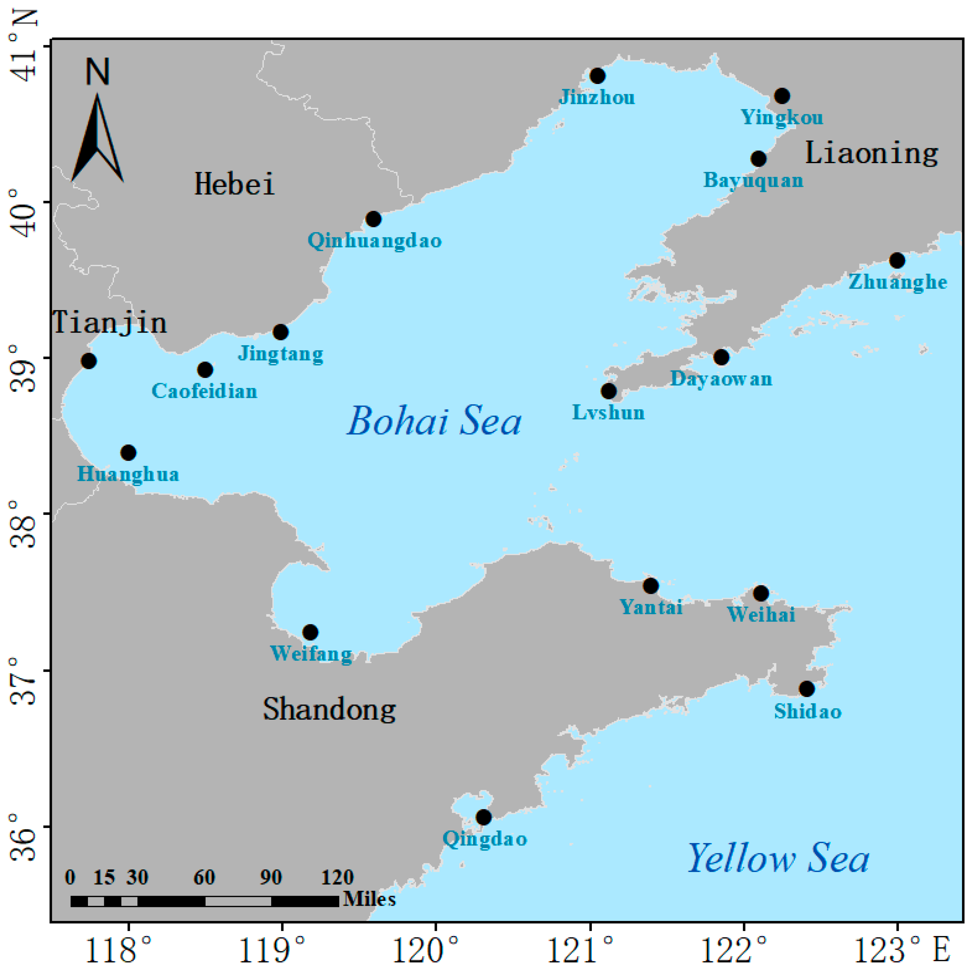
Figure 1. Study area.
Remotesensing 13 03530 g001
Figure 2. Flow chart of the navigation risk evaluation method.
Remotesensing 13 03530 g002
Figure 3. Flow chart of sea fog identification method.
Remotesensing 13 03530 g003
Figure 4. Sample selection using CALIPSO-VFM data, (a) AHI image on 15 June 2018 at 05:10 UTC. (b) Objects classification of CALIPSO-VFM data from 15 June 2018 at 05:17 UTC.
Remotesensing 13 03530 g004
Figure 5. Spectral analysis, (a) the spectral reflectivity of bands 1–6 and NDSI for AHI data; (b) the brightness temperature of bands 7–16 for AHI data, the red box represents the regions of bands 13, 14, and 15 with obvious differences in brightness temperature of each objects.
Remotesensing 13 03530 g005
Figure 6. Distribution of accident points.
Remotesensing 13 03530 g006
Figure 7. Shipping route distribution.
Remotesensing 13 03530 g007
Figure 8. Channel area division process, (a) the simplified shipping routes and points; (b) the regional Tyson polygon using Delaunay triangulation method with route points as the source; (c) shipping route areas after merging and trimming.
Remotesensing 13 03530 g008
Figure 9. Distribution of CALIPSO-VFM verification points around UTC 05:00 from January to September in 2018.
Remotesensing 13 03530 g009
Figure 10. Frequency distribution of sea fog in (a) spring; (b) summer; (c) autumn; (d) winter.
Remotesensing 13 03530 g010
Figure 11. Navigation risk assessment and accident points matching results in (a) spring; (b) summer; (c) autumn; (d) winter.
Remotesensing 13 03530 g011
Figure 12. Sensitivity analysis results.
Remotesensing 13 03530 g012
Figure 13. Risk distribution in the waterway areas in (a) spring; (b) summer; (c) autumn; (d) winter.
Remotesensing 13 03530 g013
Table 1. Data information.
NameSourceData DescriptionTimePurpose
AHI dataJapan Aerospace Exploration Agency
(https://www.eorc.jaxa.jp/ptree (accessed on 1 July 2021))
Remote sensing images from the AHI sensor [10]2015–2020Sea fog identification and calculating the frequency of monthly sea fog
CALIPSO-VFMNational Aeronautics and Space Administration
(https://search.earthdata.nasa.gov/search (accessed on 7 July 2021 ))
Classified data of clouds and aerosols from CALIPSO lidar level-2 product [27]2018Sea fog samples and verifying the accuracy
Wind European Centre for Medium-Range Weather Forecasts
(https://www.ecmwf.int/ (accessed on 15 June 2021))
10 m wind reanalysis data from ERA5 [28]2015–2020Calculating the frequency of strong wind
Sea waveEuropean Centre for Medium-Range Weather Forecasts
(https://www.ecmwf.int/ (accessed on 15 June 2021))
Significant Wave Height reanalysis data from ERA5 [28]2015–2020Calculating the frequency of big waves
Ocean currentsNational oceanic and atmospheric administration
(https://www.ncei.noaa.gov/ (accessed on 16 June 2021))
Analyses currents data from HYCOM [29]2016–2020Calculating the frequency of big currents
Water depthBritish Oceanographic Data Centre
(https://www.bodc.ac.uk/ (accessed on 16 June 2021))
Global terrain model from GEBCO [30]2019Obtaining water depth data
Accident dataMaritme Safety Admininstration of the people’s Republic of China
(https://www.msa.gov.cn/ (accessed on 1 March 2021))
Accident data collected and disclosed by the authorities2015–2020Weighting factors and validating the risk model
Shipping routesMaritme Safety Admininstration of the people’s Republic of China
(https://www.msa.gov.cn/ (accessed on 1 March 2021))
Officially recommended shipping route [31]2019Subdivision shipping route
Table 2. Statistics of accident-related factors.
FogWindWaveCurrentsWater DepthRainfallTotal
Number13171879468
Proportion19.2%25.0%26.5%10.3%13.2%5.8%100%
Ranking321546
Table 3. Correlation table of CRITIC-determined weights.
WindWaveSea FogCurrentsWater Depth
Wind10.76−0.150.230.19
Wave0.761−0.170.040.12
Sea fog−0.15−0.171−0.01−0.12
Currents0.230.04−0.011−0.21
Depth0.190.12−0.12−0.211
Table 4. Weights.
Table 4. Weights.
NameWindWaveSea FogCurrentsWater Depth
R z 2.973.244.463.954.02
CRITIC weights0.140.170.360.170.14
Final weights0.190.230.370.090.10
Rank32154
Table 5. Confusion matrix of sea fog classification.
Sea FogNon-Sea Fog
HF
Sea fogMLP8817
NDSI9675
MC
Non-sea-fogMLP20206
NDSI12148
Table 6. Accuracy of sea fog classification.
MethodsPODPMDPFDETS
MLP81.48%7.62%18.51%59.22%
NDSI threshold88.89%33.63%11.11%31.61%
Table 7. Accident matching table.
SpringSummerAutumnWinterSummary
Success666220
All accident numbers878629
Matching rate75%85%75%33%69.9%
Publisher’s Note: MDPI stays neutral with regard to jurisdictional claims in published maps and institutional affiliations.