Article

Integration of Remote Sensing Data into a Composite Voxel Model for Environmental Performance Analysis of Terraced Vineyards in Tuscany, Italy

by
Jakub Tyc
1,*,
Defne Sunguroğlu Hensel
2,
Erica Isabella Parisi
3,
Grazia Tucci
3 and
Michael Ulrich Hensel
1
1
Research Department for Digital Architecture and Planning, Vienna University of Technology, Karlsplatz 13, A-1040 Vienna, Austria
2
Green Technologies in Landscape Architecture, Technical University Munich, Arcisstrasse 21, 80333 Munich, Germany
3
Laboratory of Geomatics for Environment and Conservation of Cultural Heritage (GeCo), Department of Civil and Environmental Engineering, University of Florence, Via di S. Marta 3, 50139 Florence, Italy
*
Author to whom correspondence should be addressed.
Remote Sens. 2021, 13(17), 3483; https://doi.org/10.3390/rs13173483
Submission received: 8 July 2021 / Revised: 25 August 2021 / Accepted: 30 August 2021 / Published: 2 September 2021
(This article belongs to the Section Remote Sensing in Agriculture and Vegetation)

Abstract

:
Understanding socio-ecological systems and the discovery, recovery and adaptation of land knowledge are key challenges for sustainable land use. The analysis of sustainable agricultural systems and practices, for instance, requires interdisciplinary and transdisciplinary research and coordinated data acquisition, data integration and analysis. However, datasets, which are acquired using remote sensing, geospatial analysis and simulation techniques, are often limited by narrow disciplinary boundaries and therefore fall short in enabling a holistic approach across multiple domains and scales. In this work, we demonstrate a new workflow for interdisciplinary data acquisition and integration, focusing on terraced vineyards in Tuscany, Italy. We used multi-modal data acquisition and performed data integration via a voxelised point cloud that we term a composite voxel model. The latter facilitates a multi-domain and multi-scale data-integrated approach for advancing the discovery and recovery of land knowledge. This approach enables integration, correlation and analysis of data pertaining to different domains and scales in a single data structure.

Graphical Abstract

1. Introduction

Advancing the understanding of socio-ecological systems is a key challenge for sustainable development. This necessitates interdisciplinary [1,2] and transdisciplinary [3] approaches. However, analysing complex dynamic systems from an integrative perspective, thereby facilitating improved comprehension of the interactions of sustainable agricultural systems and practices with their environments and their impact on one another, constitutes a considerable challenge. Addressing the recovery and adaptation of land knowledge requires data integration across a range of disciplines. In the context of our research, this includes agronomy, biology, soil science, hydrology, microclimatology, and environmental science, as well as expert knowledge in data acquisition, data science and information modelling. To progress beyond the limits of discipline-specific approaches, it is necessary to develop a consolidated interdisciplinary approach for targeted data acquisition, correlation and integration. In this article, we present a new workflow that combines (1) multi-source remote sensing data, (2) data from open source geographic information systems (GIS), (3) data obtained from simulations and (4) the integration of the obtained datasets into a voxelised point cloud, which we term a composite voxel model (CVM), which enables targeted inquiry for land knowledge recovery.
The primary goal of this article is hence to present a data-integration approach based on the use of a composite voxel model. To make this approach tangible, we discuss it with focus on the thermal performance analysis of high-altitude terraced vineyards in Lamole, Tuscany, Italy. This is done with the aim of demonstrating how a multi-scale analysis can be facilitated.
The land knowledge inherent in the terraced landscapes of Tuscany has been recognised by UNESCO as an ‘Intangible Cultural Heritage of Humanity’ [4]. The unique value of terraced landscapes and their contribution to sustainability has been acknowledged by the UN’s Food and Agriculture Organisation in the context of ‘Globally Important Agricultural Heritage Systems’ [5]. Terraced vineyards in Tuscany frequently combine terrain modulation and construction, as well as plant manipulation. Terraces provide flat terrain, mitigation of landslides and soil erosion, effective water management and provision of a microclimate that is beneficial to agriculture and viticulture [6]. Terracing is often accompanied by the use of dry-stone walls, which provide slope and drainage management and modulate microclimate [7]. The traditional knowledge that underlies this type of viticulture enables resilient solutions that are often coupled with adaptation strategies for climate change or technological developments. However, interdisciplinary research on knowledge recovery and adaptation, particularly pertaining to the environmental performance of terraced vineyards, is still sparse [8].
In the context of viticulture, geospatial analysis methods have been applied to detect terraced landscapes from digital elevation models (DEMs) and unmanned aerial vehicle (UAV) data [9]. Stubert et al. integrated expert knowledge with geospatial analysis methods for studying the distribution of ancient wine-pressing facilities of Roman viticulture using predictive computational modelling [10]. The role of terraced landscapes in preventing soil degradation [11] and the negative impact of land abandonment and degradation have been studied [12]. Hydrological aspects have been investigated at different scales through remote sensing and geomatic methods. High resolution DEMs derived from photogrammetric acquisitions and terrestrial laser scanning point clouds have been combined with GIS and simulation tools to study the hydro-geomorphological characteristics of terraced vineyards and develop strategies for mitigating erosion caused by surface water [13,14,15,16]. Some studies presented a comparison of remote sensing with a field survey for soil moisture content assessment and prevention of terrace damages [17]. Other studies have involved the geo-typological features of dry-stone walls in Tuscany [7], and more recently, the environmental performance of terraced vineyards in Lamole [18,19,20,21,22].
However, an integrated interdisciplinary approach for comprehensive land knowledge recovery, i.e., a holistic understanding of the dynamic interactions of terraced vineyards with their environments, is currently lacking. This type of research entails coordinated multi-modal data acquisition, integration and analysis across multiple scales from the territorial scale to the scale of an individual vineyard to individual features, such as dry-stone walls, plants or green borders of vineyards, as shown in Figure 1.
The integration of data acquired through remote sensing methods coupled with geospatial simulations was applied in this study for environmental performance evaluations from the territorial scale to site and feature scales. We particularly focused on the thermal performance of the terraced vineyards to quantitatively assess terrace-induced microclimate variations, which impact vine plant growth, ripening and yield and, thus, the final quality of the produced wine. Methodological considerations on thermal data acquisition and processing procedures have been portrayed in previous articles [20,21,22] or are currently under review.
In this article, we present a novel approach for the spatial and temporal integration of remote sensing data and GIS methods related to solar performance into a CVM, which involves a convergence of point clouds and 2.5D geoscientific datasets. The data used as inputs were generated using remote sensing methods, which provided multi-resolution geomorphological products and multispectral information (visible and thermal). Furthermore, geoscientific solar analysis and its three-dimensional equivalent, also associated with the domain of digital architecture, were implemented. The presented method enables the correlation of different datasets that are not easily comparable because of the diversity of discipline-specific approaches and non-interoperable methodologies and tools. Overall, we aimed to gain insight into the unique environmental performance of terraced vineyards in Lamole in order to integrate it into subsequent steps with data-driven design and decision support for the adaptation of recovered land knowledge relating to various contexts.
In the results section, we describe the interdisciplinary approach to data acquisition that was adopted for the survey campaigns of terraced vineyards in Lamole. The results of the photogrammetric acquisition in the visible (VIS) and thermal infrared (TIR) ranges, airborne LiDAR data, data from open-access GIS and local meteorological station data were demonstrated. We then elaborate our approach with data integration via the CVM, which incorporates data pertaining to multiple domains and spatial and temporal scales. In the discussion section, we examine our findings, especially the implications of the CVM and the related workflow. Further research questions and phases are outlined, especially with a focus on developing decision support regarding land use monitoring, which can offer further insights into sustainable development in rural areas and their broader adaptation to other rural and urban contexts.

2. Materials and Methods

Different data acquisition methods and data sources were deployed, and an approach to data integration was developed. Here, we outline the utilised remote sensing and field-based data acquisition methods, open-access GIS data implementation and the developed CVM for data integration.
Two study areas were selected for this research, characterized by two different site morphologies: the Castello vineyard and the Grospoli II vineyard. The Castello vineyard is located at the entrance to the Lamole valley at a medium altitude of 525 amsl and features terraced (~0.5 ha) and non-terraced (~1.65 ha) areas. The terraced area, exposed to N–NE, is made by a combination of dry-stone walls and ledges as structural elements. The Grospoli II vineyard (~1 ha) is located deeper in the Lamole valley at a higher altitude (630 m amsl) and on a steep slope. The vineyard is oriented in the N–S direction, divided into two sections by a central drainage channel and comprises six dry-stone walled terraces and one ledge.
The difference in altitude and orientation of the two vineyards provided individual and comparative solar performances simulations and thermal data acquisition. However, the Grospoli II vineyard is the primary case study. Furthermore, these two vineyards established the site scale, whereas the entire Lamole valley established the territorial scale.

2.1. Remote Sensing Data Acquisition

Different remote sensing platforms were used for surveying the study area at different scales to identify a representative set of vineyards for closer investigation. An overview of the different flights is shown in Table 1.

2.1.1. Airborne LiDAR and Photogrammetric Flight

An airborne photogrammetric and LiDAR flight was performed on 6 August 2020, over the entire Lamole valley, to provide territorial scale data. The flight was performed by the Servizi di Informazione Territoriale (S.I.T.) s.r.l. of Bari (Italy), and the aircraft was equipped with a Phase One iXU-RS-1000 RGB camera (100 MP, 50 mm focal length). The photogrammetric flight plan was designed to cover an area of approximately 340 ha and obtain a ground sample distance (GSD) of 6–7 cm. The flight pattern consisted of 3 swipes and 48 frames, with forward overlapping > 70%. The images were acquired with a nadiral camera at a constant speed of 50 m/s and an altitude of 1000 m above ground level (AGL). The aircraft also mounted a LiDAR sensor Riegl Q680i, which operated at 400 kHz with a 60° field of view, a point density average of 4–6 pt/m² and 3 multiple-time-around zones. For each echo-signal, high resolution 16-bit intensity information was provided for the visible and near-infrared spectral bands (RGBI). The orientation of the photogrammetric and LiDAR data was registered thanks to the Novatel IMU-FSAS inertial system and the global navigation and satellite system (GNSS) receiver, SPAN SE, connected to all the acquisition equipment. Ten ground control points (GCPs) were additionally used for georeferencing the image flight. Further specifications are reported in Table 1.

2.1.2. Visible and Thermal Infrared Flights of Unmanned Aerial Vehicle (UAV)

On the scale of individual vineyards, existing RGB-TIR photogrammetric acquisitions [20,21] were extended with further surveys using a UAV platform integrating both visible and thermal sensors (DJI Mavic 2 Enterprise Dual). A complete overview on the methodological evolution for thermal data acquisition is already reported in [22]. A comparison between the technical details of the different surveys is reported in Table 1.
Five flights with a temporal resolution of 3 hours were performed over the study area (Grospoli II vineyard) on 5 September 2020. The photogrammetric data capture was performed simultaneously in the VIS and TIR range. The used UAV platform was a multirotor quadcopter, which can be remotely controlled and programmed for automatic navigation, provided by GNSS waypoints. The UAV had a maximum take-off weight of about 1100 g and a diagonal size of 354 mm with a maximum flight time of approximately 30 min and a maximum speed of 72 km/h. The Mavic 2 Enterprise Dual was equipped with an integrated sensor system for the RGB range (M2ED) and the TIR range (FLIR Lepton 3.5) and was stabilised with a 3-axis (pitch, roll, yaw) gimbal. The RGB camera used a 1/2.3’ CMOS 12 MP sensor with a maximum resolution of 4056 × 3040 px. The fixed focal length was 35 mm (format equivalent of 24 mm) with 85 FOV and f/2.8. The TIR camera was not radiometrically calibrated and had a sensor resolution of 160 × 120 px with a 57° horizontal field of view. The focal plane array image sensor was made of uncooled microbolometers (12 × 12 μm each) with a spectral TIR response in the range 8–14 μm and accuracy of ±5 °C or 5%. The camera provided thermal images of 640 × 480 px in JPEG format.
The photogrammetric flight plan was designed with the Dronelink software by setting the suitable parameters to have a GSD of approximately 2 cm. The flight plan consisted of 14 swipes with forward overlapping of 80% and sidelap of 70%. The images were acquired with a nadiral camera at a constant speed of 3.4 m/s and an altitude of 60 m AGL. Further flights with tilted cameras at 60° were performed to acquire the vertical structures of the terraces. The georeferencing of the photogrammetric survey was made using 22 GCPs, which guaranteed the metric accuracy of the survey. The targets were homogeneously distributed around the surveyed vineyard to cover all the involved surfaces. The positioning and measuring activities for each target were performed by the GNSS. A multi-frequency receiver (Emlid Reach RS2) was used for the coordinate’s acquisition in the networking real-time kinematic (NRTK) mode and with accuracies on the order of centimetres. The coordinate system used in all data processing was ETRS89/UTM32N (EPSG: 25832). Photogrammetric data was generated with an open source photogrammetric reconstruction workflow based on MicMac [23] and COLMAP [24]. Keypoint extraction and matching, as well as the initial structure from motion (SfM) reconstruction, was conducted by COLMAP using SiftGPU, vocabulary tree matching [25] and multithreaded incremental SfM implementations. NRTK-GNSS based georeferencing of the scene and coordinate system reprojections, as well as the final dense point cloud reconstruction steps, were conducted in MicMac.
A detailed description of the photogrammetric data processing will be provided in an upcoming publication.

2.2. Field Data Collection and Open-Access Geographic Information Systems (GIS) Data

To further extend the content of the CVM, field data and regional open-access geospatial information were required. The Tuscan GIS database was used to encode land use classifications into the CVM. Outcomes of the solar radiation simulation were validated with the pyranometer data collected by the local meteorological station. Ground-based reference temperature measurements were also collected to integrate multi-scale data correlation.

2.2.1. Field Data Collection

A control system was set up on the field to cross-check the temperature values obtained from the TIR-UAV survey with ground truth. Specific aluminium target panels (50 × 50 cm) were designed to detect in the TIR range (low emissivity of aluminium) and contained a contact sensor (thermocouple) for measuring temperature reference values. A pre-flight calibration was performed before each flight over these panels [26]. Those reference values were used to compare the temperature measured with the non-radiometric TIR sensor integrated into the UAV platform with the temperature measured thermocouple sensors. Moreover, data from the Lamole meteorological station (TOS11000023), operated by the Servizio Idrologico Regionale (SIR) of the Tuscan Region, was used to validate the simulation outcomes in the site scale, as described in Section 3.2.2. At the same time, global horizontal irradiance (GHI) was used for the three-dimensional solar simulation on the feature scale, which is described in Section 3.3.3.

2.2.2. Open-Access Geographic Information Systems (GIS) Data

Open-access GIS data were used to augment LiDAR data with spatial planning information. Information on land use contained in the Geoscopio Portal of Regione Toscana served to locate all vineyards in the Lamole valley. Data were made available in a vector-based format compatible with QGIS (Quantum GIS 2.18). Further processing and rasterisation of the open-access GIS data were done in QGIS.

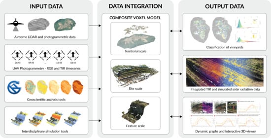
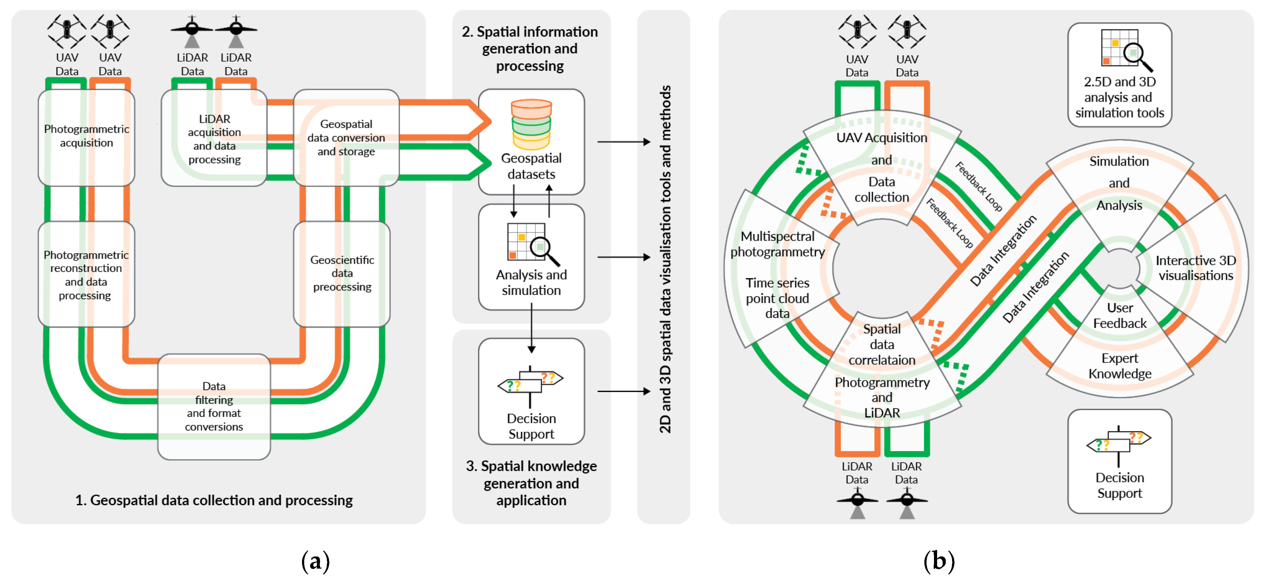
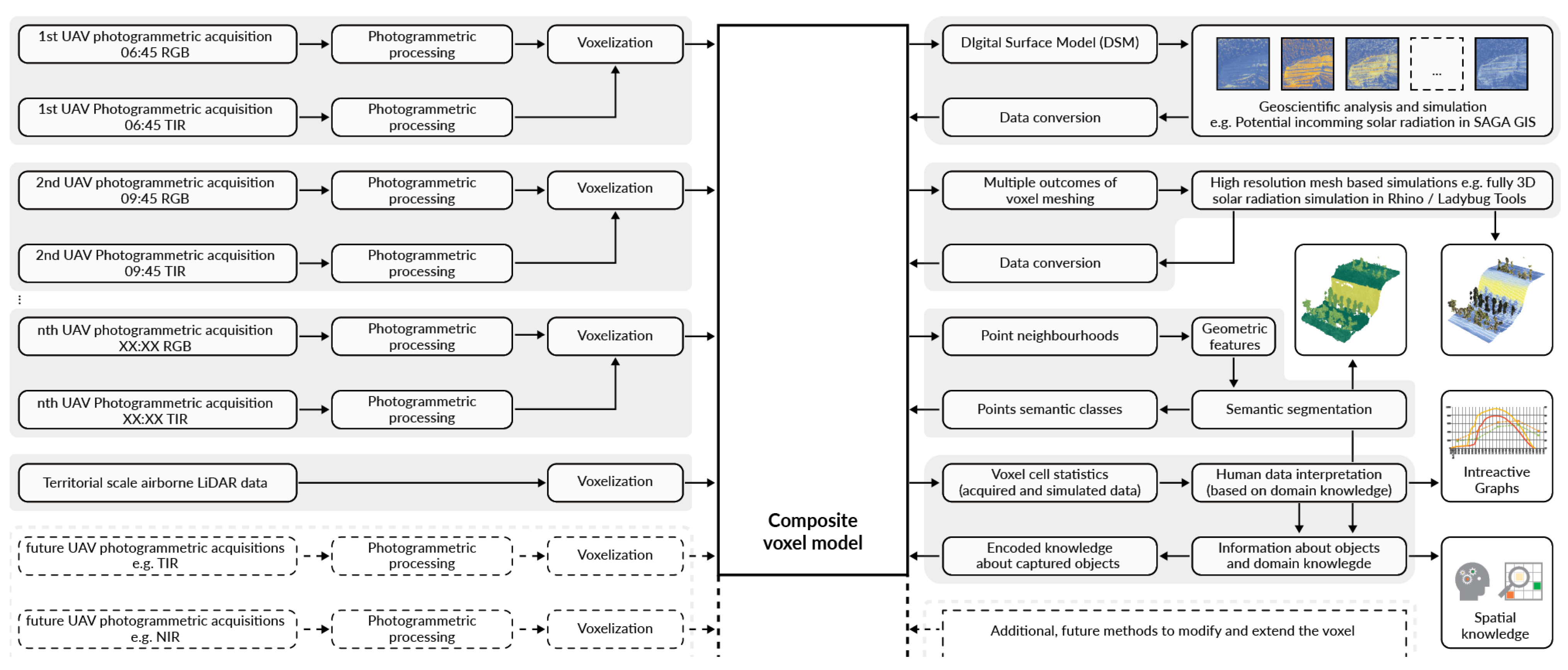
2.3. Composite Voxel Model (CVM)

A voxel model is a spatial representation of data that stores and visualises extended parameters assigned to individual data points, so-called voxel cells that are structured as a three-dimensional grid. In geospatial science, voxel models are typically used to extract canopy height models [27], single tree detection [28] and leaf area density estimation from airborne LiDAR data [29]. More recently, the use of voxels for interdisciplinary spatial data integration was explored in the PANTHEON project [30]. The aforementioned project is developing integrated supervision and data acquisition system aimed at precision agriculture in hazelnut orchards. Both terrestrial and aerial autonomous robotic platforms are constantly collecting large quantities of geospatial data, which are centrally processed to support the execution of common orchard maintenance tasks, such as irrigation. The need for interdisciplinary data integration resulted in the publication of a pyoints python library [31], which bridges different representations of geometric point-based data, including point clouds and geo-referenced rasters, as well as the voxels required by the prototype of farming robots aimed at precision agriculture applications [32].
The fusion of multi-spectral image data and high resolution point clouds to create multi-temporal, information-rich spatial models pose a challenge. Jurado et al. [33] created a multi-spectral and multi-temporal photogrammetric point cloud model for the characterisation of individual olive trees that makes it possible to calculate and visualise three-dimensionally vegetation indices. Based on this, multidimensional data information on single plants can be extracted and visually and statistically evaluated to monitor the development of olive trees. Plant analysis was conducted in the multi-temporal dataset with a voxel-based single plant segmentation method.
Point-based data formats, such as point clouds, 2.5D georasters, data cubes and structured grids produced with computational fluid dynamics (CFD) simulations are commonly utilised in remote sensing and different simulation methods. However, interdisciplinary and interoperable implementations are still uncommon. Point clouds are unstructured, three-dimensional, geo-referenced datasets, often of varying density. The conversion of point cloud into a geospatial 2.5D raster format transforms 3D points into a regularly spaced grid of cells, where a single height value is assigned to each cell in the grid. The simulation of natural processes related to solar exposure or surface flow accumulation was conducted using open source packages, such as QGIS [34] and SAGA GIS [35], based on 2.5D raster data.
A data cube is a multi-spectral dataset constructed from publicly available multi-temporal earth observation datasets, such as Landsat, Sentinel and MODIS. These satellite data contain, among other things, TIR data in the spatial resolution measured in tens or hundreds of metres [36]. Datasets collected in the data cube are structured in a multidimensional grid where, conventionally, change in time is mapped to the third dimension, and different layers of information are assigned to higher dimensions [37]. Due to the large data quantities contained in data cubes, python data science tools such as Dask [38], XArray [39] and scikit-learn [40] are often applied to work with data cubes. On a smaller scale, the impact of environmental factors, such as wind, can be simulated with CFD at the scale of a building [41] or landform [42]. Outcomes are visualised as spatial grids. The grid dimensions depend on the simulation parameters and do not contain external simulation data, such as captured physical objects with real-world colours, as is the case of point data encoded in photogrammetric point clouds.
Our CVM was derived by structuring the photogrammetric point cloud as a three-dimensional grid in a process called voxelisation or gridding. CVMs generate an interface by applying established remote sensing methods to a custom-made dataset. This expands the scope of the analytical and simulation tools used for the geoscientific analysis of the territorial scale to integrate data pertaining to the territorial scale, the site scale (a single vineyard) and the feature scale (e.g., a single dry-stone wall or plant). The voxelisation of geo-referenced point clouds unifies the point density while preserving the three-dimensional information. A bidirectional link with 2.5D geospatial analysis tools was established through existing python interfaces integrated into open source tools. Complimentary tabular representation of high-dimensional data enables the application of python-based machine learning (ML) methods for point cloud semantic segmentation and the study of environmental conditions in the vineyards. Because voxelisation preserves the three-dimensional information, it was possible to integrate a three-dimensional solar simulation of the solar performance of the dry-stone walls. This was implemented in Ladybug Tools [43]. Therefore, the time series TIR data collected with the UAV platform and the simulated solar radiation could be correlated in the CVM.
A large amount of data and computational capacity is required for the correlation of this high-dimensional dataset resulted in the application of tools used for data cube processing (e.g., Numpy, Pandas and Dask). These tools were used for point cloud voxelisation to combine multiple TIR and RGB point clouds into one CVM and integrate it with airborne LiDAR data. This workflow enables a variety of data representations, i.e., combining an interactive 3D point cloud viewer with dynamically updated graphs, providing intuitive data exploration and interpretation.

3. Results

In this section, we portray the introduced processes and methods of data acquisition and data integration applied to high-altitude terraced vineyards in Lamole. To move towards a trans-scalar data integration, we collected data relative to three different scales: (a) the territorial scale of the Lamole valley, (b) the site scale comprising individual vineyards and (c) the feature scale comprising individual dry-stone walls or vine plants.

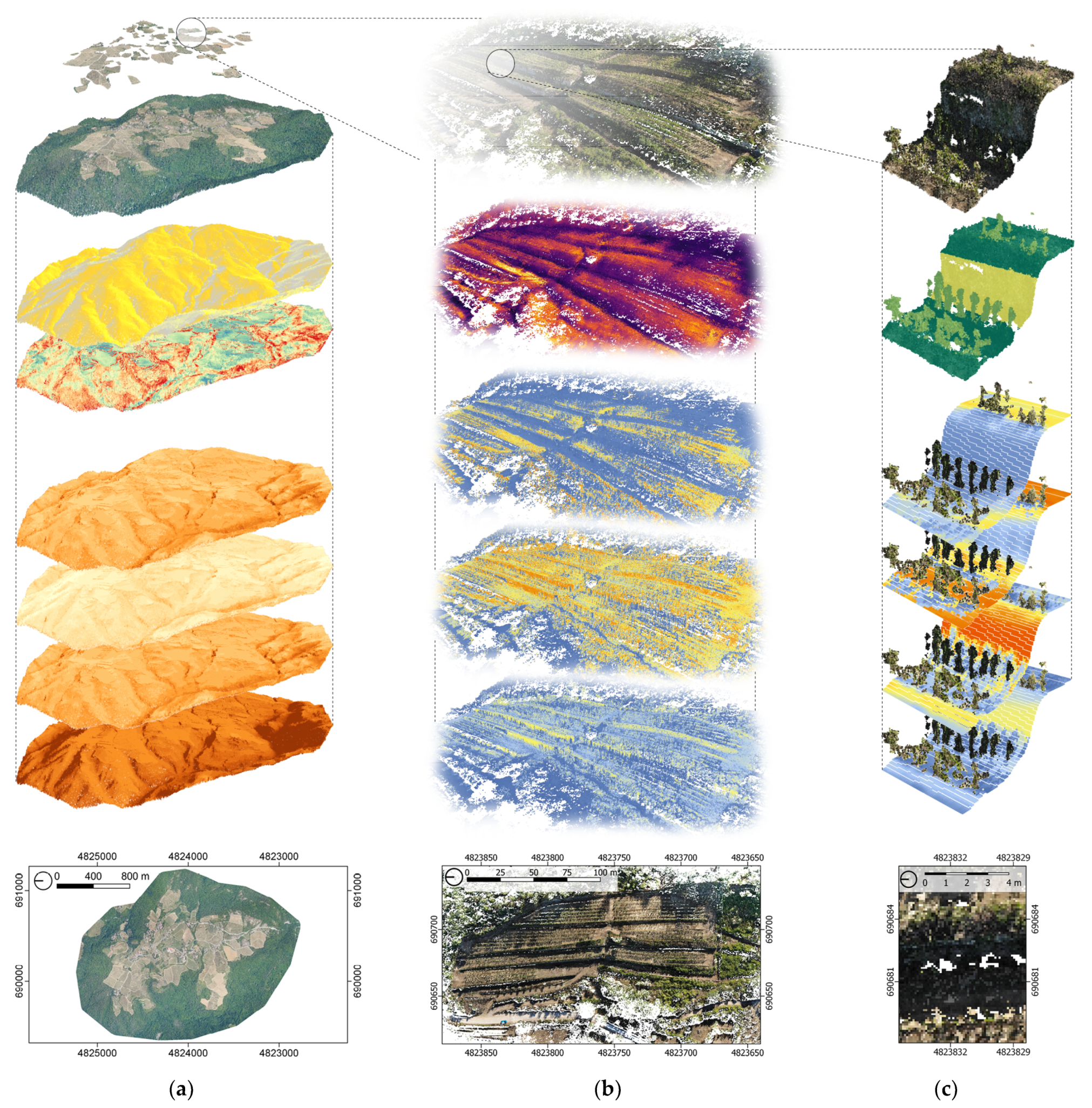
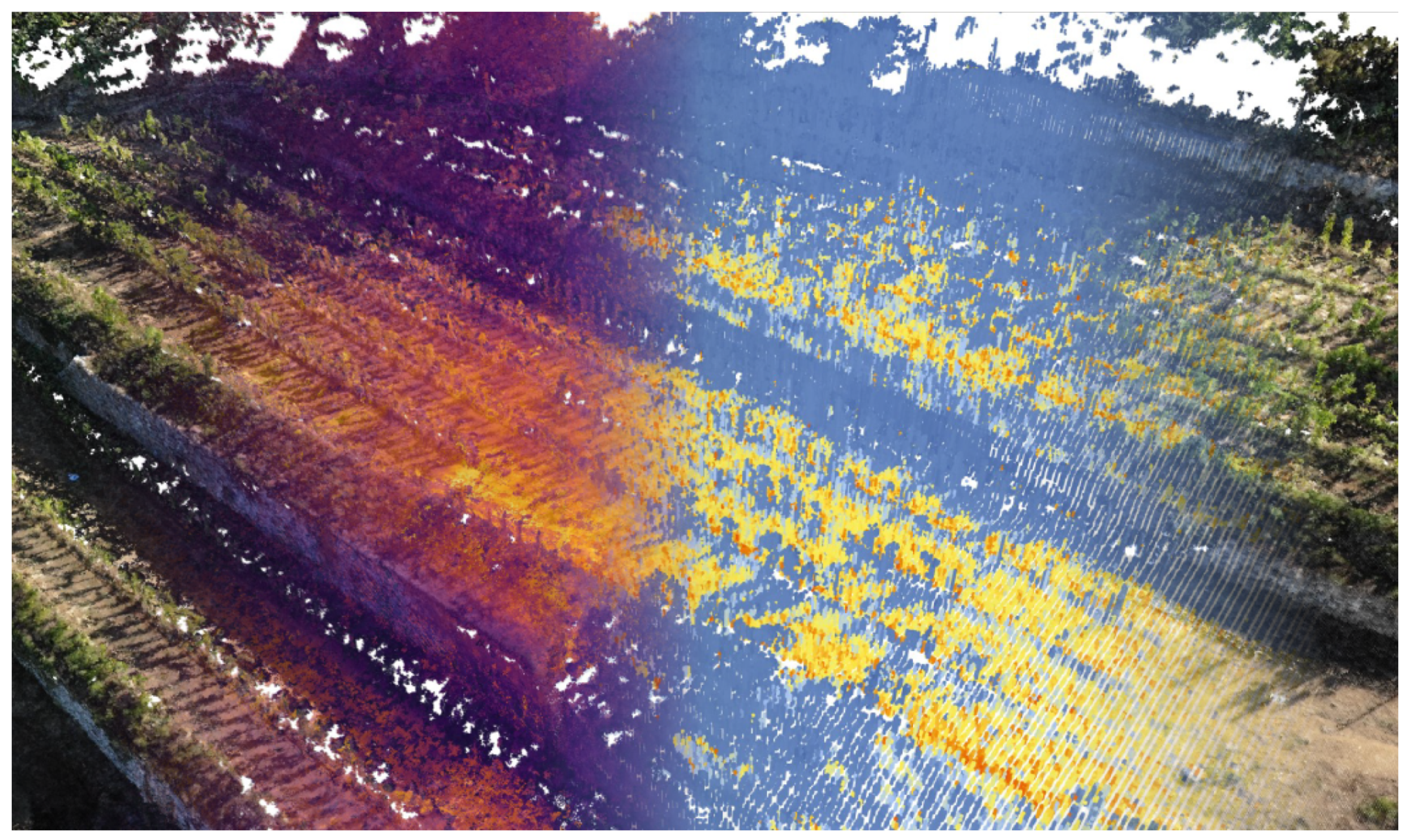
3.1. Remote Sensing Data Integration

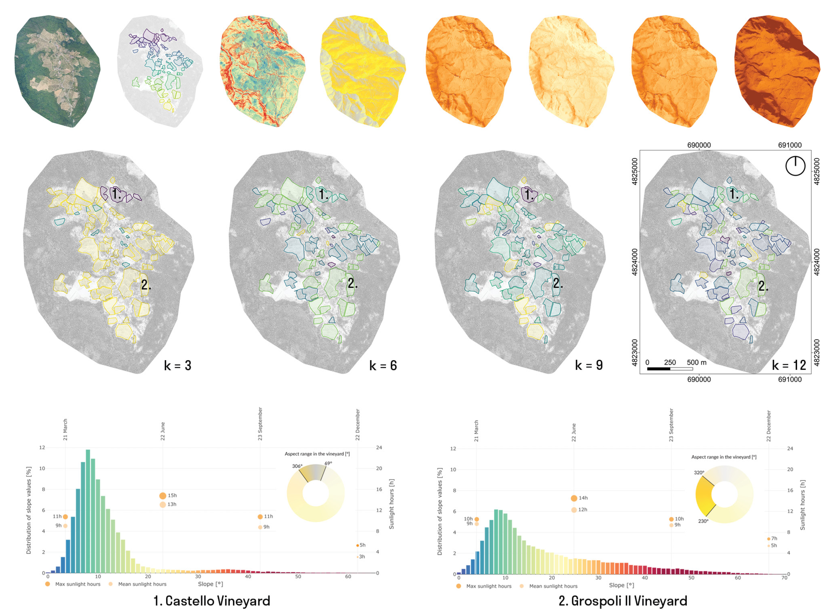
3.1.1. Territorial Scale

The outputs of the airborne LiDAR survey, provided by S.I.T. s.r.l., consisted of an RGB point cloud containing classification information, a digital terrain model (DTM) and a digital surface model (DSM), both with a resolution of 50 cm GSD. This dataset covered the entire Lamole valley and was used to study the distribution of environmental parameters at the territorial scale. Furthermore, it was used to substitute the missing data on the vegetation surrounding the selected vineyards. An orthophoto of the valley was produced as a result of the photogrammetric airborne flight (6–7 cm GSD) that was used to provide the RGB values to the LiDAR point cloud.

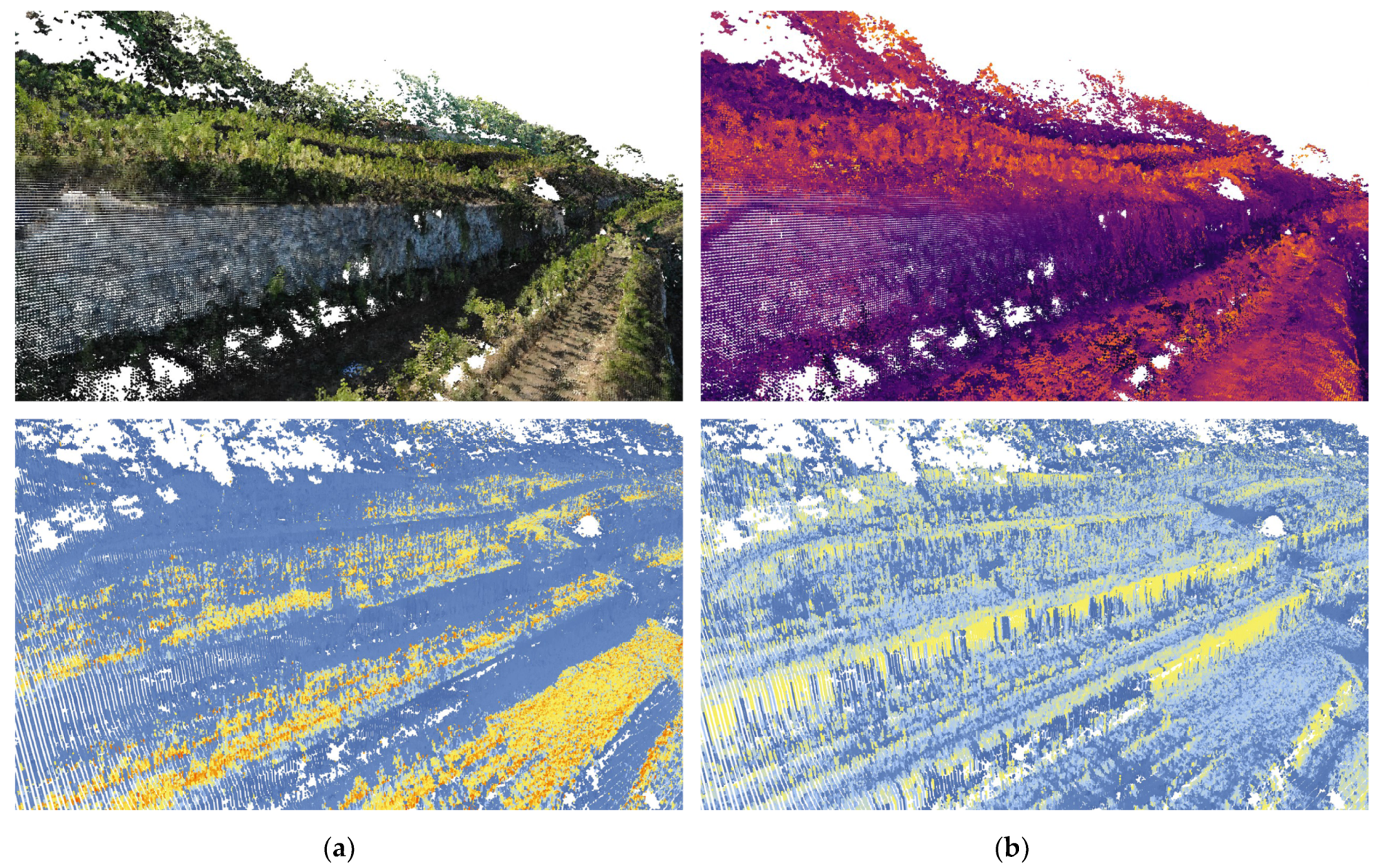
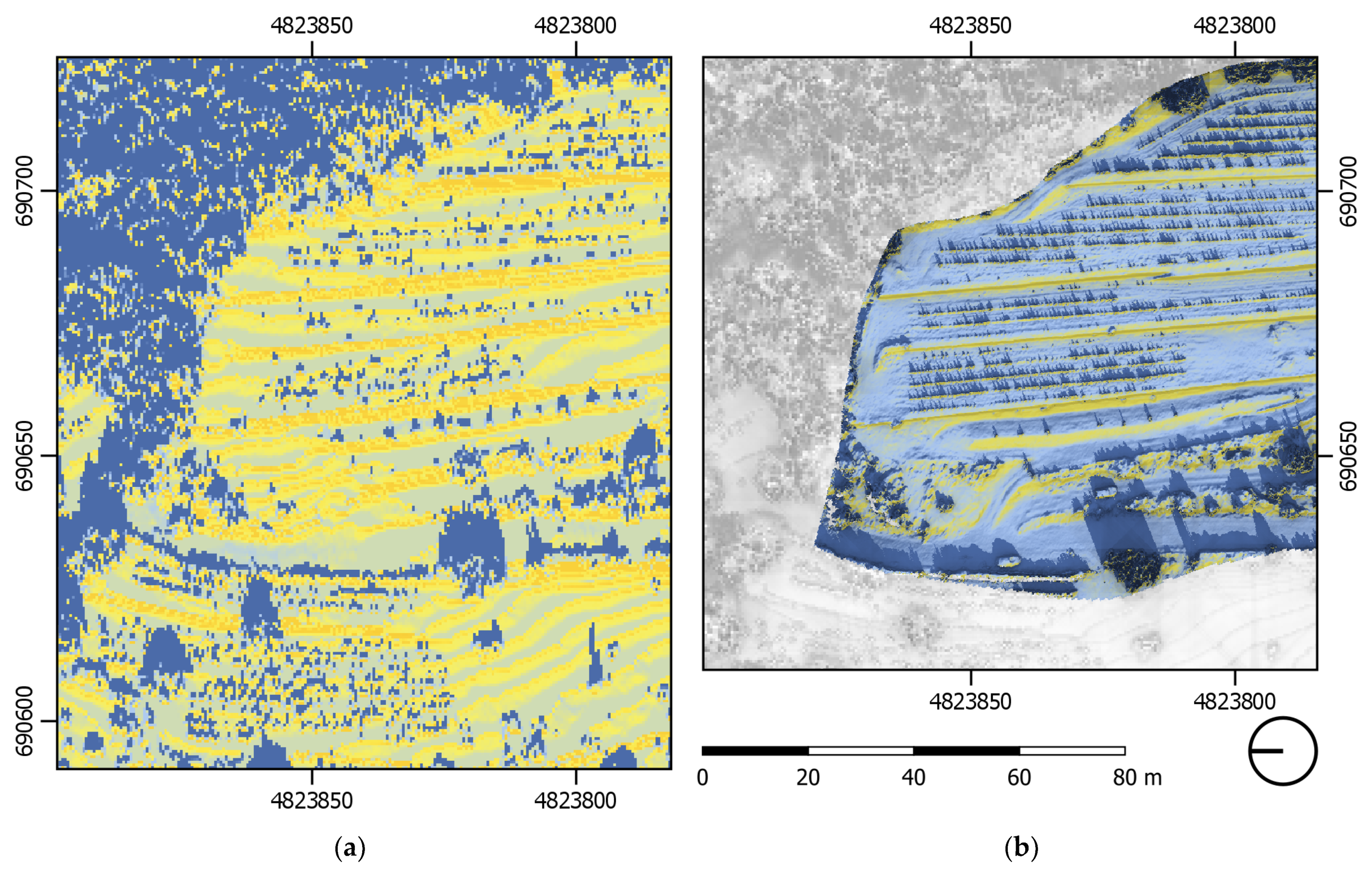
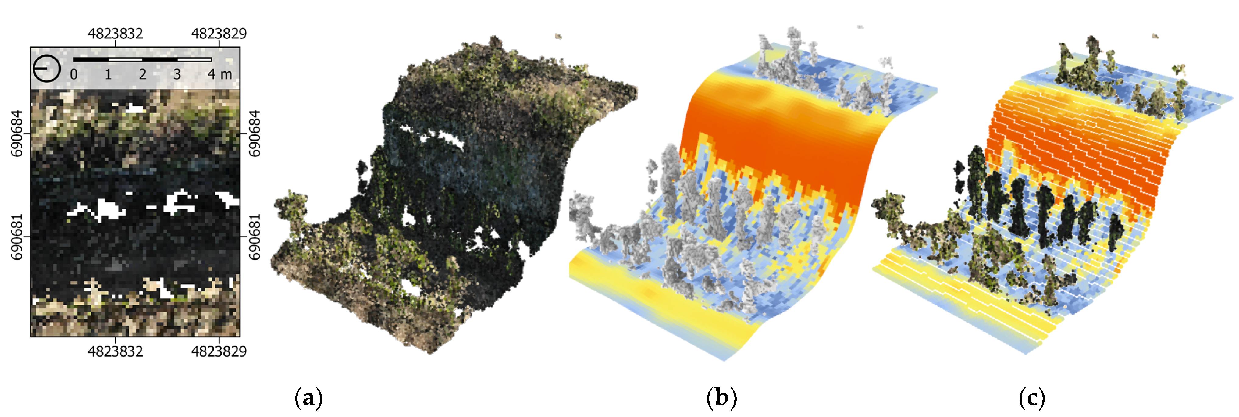
3.1.2. Site and Feature Scale

Surveys conducted with the DJI Mavic 2 Enterprise Dual platform and the photogrammetric reconstruction resulted in multiple, georeferenced point clouds. For each of the five acquisitions executed in one day, both RGB and TIR data were generated. The key parameters describing the generated photogrammetric point clouds are presented in Table 1 in Section 2.1.2. The data collected with the non-radiometric TIR sensor required additional processing and validation with a ground-based control system consisting of aluminium targets coloured in black, grey and white. The contact temperature of the aluminium targets was regularly measured and used in the pre-processing of the TIR point clouds. The outcomes of the UAV TIR survey combined with ground-based TIR data are currently being processed. Photogrammetric data was collected in the spatial resolution of 2 cm GSD in comparison with the 6–7 cm GSD of the airborne photogrammetric data. Solar radiation simulations were made with high resolution photogrammetric data to address the site and feature scales.

3.2. Open-Access Geographic Information Systems (GIS) Data and Field Data Integration

3.2.1. Territorial Scale

Locations classified as vineyards were identified based on the most recent available land use data, which was provided as open-access GIS data. The identified vineyards were matched with the results of the geospatial analysis from the LiDAR dataset. Basic analytical GIS metrics, such as the slope and aspect, were generated. Weather data from the local weather station was used to cross-check the outcomes of the incoming solar radiation analysis, as described in Section 3.3.1.
Constraints related to the limited spatial and temporal resolution of the open-access GIS data, as well as available information content, were identified. These constraints are related to changes in land use succeeding the acquisition of GIS data, as well as singular land use categories assigned to plot boundaries. The mosaic of small vineyards also contains other potentially important features, such as green corridors between the vineyards, which can strongly impact the local microclimate of a terraced vineyard. However, to evaluate their contribution at the territorial scale, land use information related to high vegetation needs to be assessed at a higher spatial resolution. Moreover, a single plot might contain both terraced and non-terraced parts, whose environmental performance metrics might differ substantially. To overcome these limitations, data acquisition at smaller scales needs to be undertaken.

3.2.2. Site and Feature Scales

Data from the meteorological station in Lamole was used to cross-check the outcomes of the solar radiation analysis of individual vineyards. Absolute radiation values measured by the meteorological station were close to the radiation values generated with the SAGA GIS analysis. SAGA GIS incoming solar radiation analysis is based on solar constant and geographic location, and the comparison presented in Figure 2 validates the applicability of this method for the dataset used in this study. The difference in the graph from 07:00 to 08:30 might be caused by the fact that the local meteorological station measures radiation with a pyranometer elevated from the ground, and the potential incoming solar radiation simulates radiation values on the ground, which starts receiving sunlight later at this west-oriented location. The meteorological station and the surveyed vineyard are located in close proximity. Their locations are marked in Figure 2 on the right. Solar radiation data from the meteorological station was also used in the three-dimensional solar radiation study to understand the solar performance of dry-stone walls in terraced vineyards. Understanding the contribution of vineyard features, such as dry-stone walls, to microclimate regulation requires targeted datasets and methods with matching scales and resolutions.

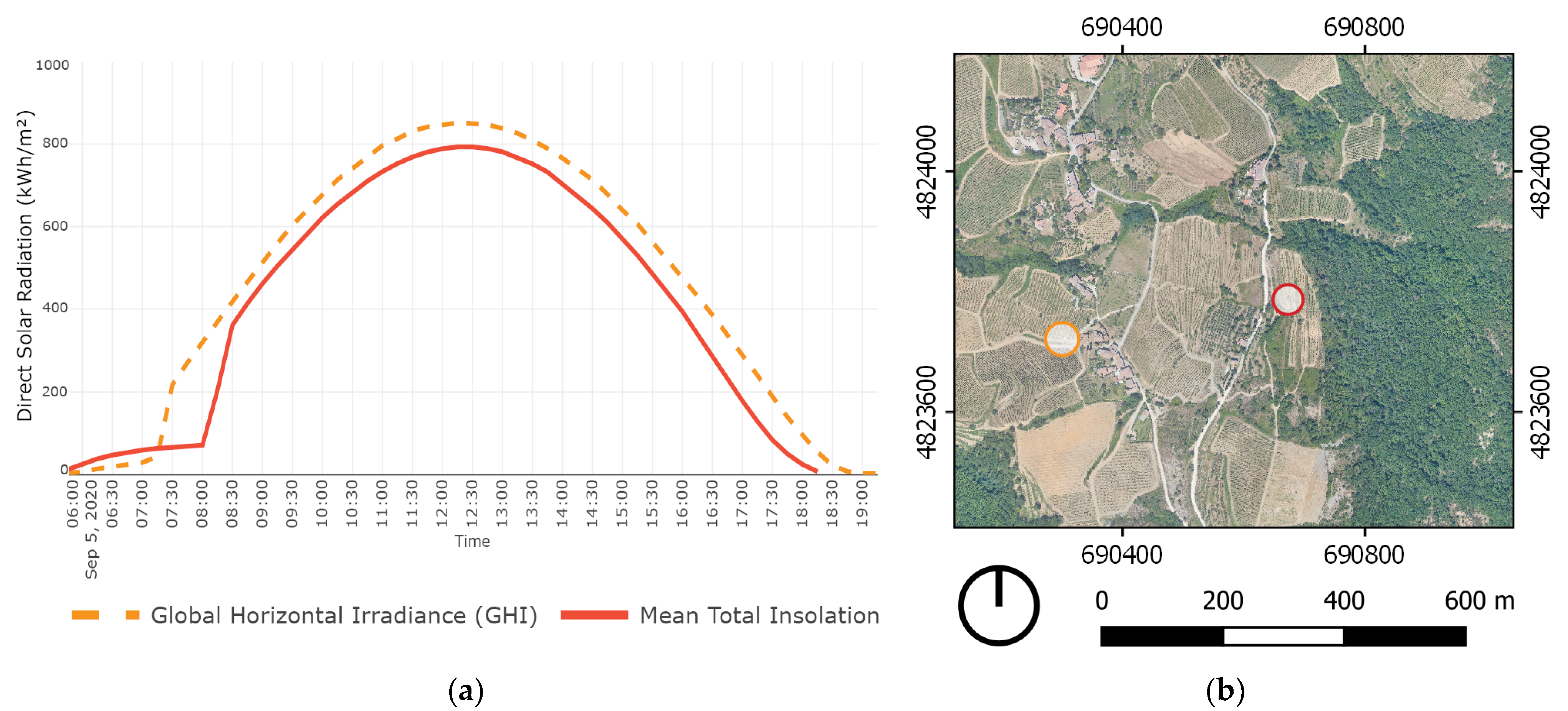
3.3. Environmental Performance Simulations

3.3.1. Territorial Scale
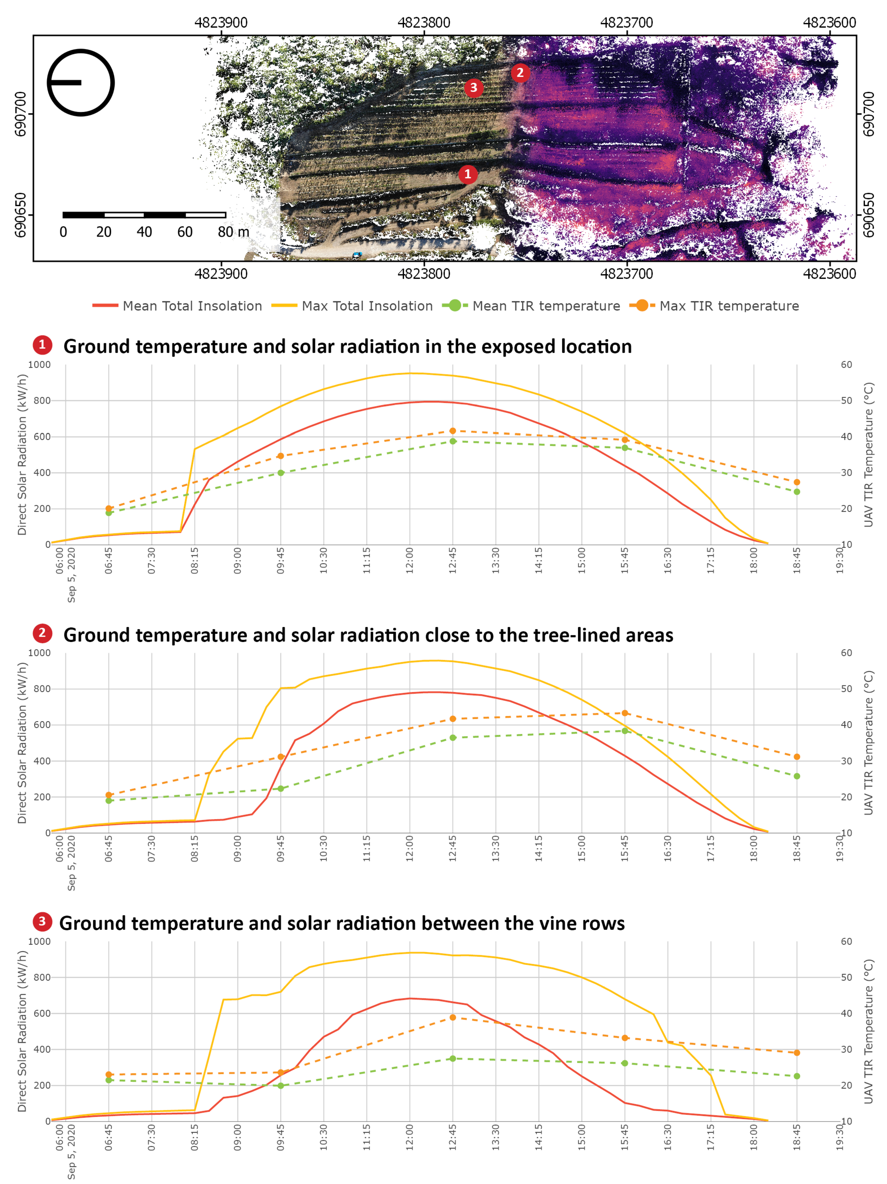
The territorial scale data used in this study consisted of airborne LiDAR data extended with spatial planning information derived from open-access GIS data. To study the solar performance of terraced vineyards at this scale, information on the insolation in matching resolution is required. Existing open-access satellite-based remote sensing data is available in moderate spatial resolution in the range of 60–120 m [36]. The potential incoming solar radiation implemented in SAGA GIS 7.7.0 [35] was applied to introduce data describing the solar performance method of the geoscientific analysis. This method [44,45,46] depends on the solar constant, a precisely geo-referenced dataset and the 2.5D description of the terrain form. Due to the simplified 2.5D representation, it is possible to work efficiently with data at the territorial scale in contrast to fully 3D simulation tools.

3.3.2. Site Scale

The same method was applied to the high resolution photogrammetric data to evaluate the solar exposure of the selected vineyard. At this scale, analysis was done for the day of the survey at a higher temporal resolution of 15-min intervals. The direct component of solar radiation was used, making it possible to focus on the moment when each point in the georaster started receiving direct solar radiation, raising the surface temperature. The validation of the results was based on data correlation from the meteorological station in Lamole with the outcomes of the simulation, as shown in Figure 2. This simulation method offers potentially unlimited time resolution when compared with a limited amount of UAV TIR acquisitions collected in one day. Efficient SAGA GIS implementation allowed setting the time interval to 15 min and completing the computation in a short time without the need for specialised computing infrastructure. In contrast, only five UAV TIR acquisitions were possible in a day due to the time needed to complete the TIR acquisition and survey logistics.
The application of the described simulation method to the dataset at two different scales and corresponding resolutions uncovered a qualitative difference related to the increased resolution. The role of dry-stone walls related to solar performance cannot be seen in the lower-resolution aerial LiDAR dataset. Only by introducing the higher resolution photogrammetric data does the environmental performance related to solar exposure become discernible. Figure 3 illustrates the qualitative difference between the two datasets.
In the airborne LiDAR dataset, the impact of dry-stone walls on solar performance can also be seen, but the difference between ground and walls is not so clear. Visual artefacts following the shape of height lines are visible due to limited resolution. This introduces non-existent height changes and causes the solar radiation values of the ground to be much higher than that in the analysis based on the photogrammetric dataset. The photogrammetric acquisition was insufficient to adequately capture the geometry of vegetation while data acquisition with LiDAR is well suited for such applications. To facilitate the comparative analysis of the TIR temperature and simulated solar exposure, both LiDAR and photogrammetric datasets were combined. This fused DSM model was based on the photogrammetric data complemented with LiDAR data for locations where photogrammetric data was not available. LiDAR data used to create the combined DSM were extrapolated to match the resolution of the photogrammetric dataset.

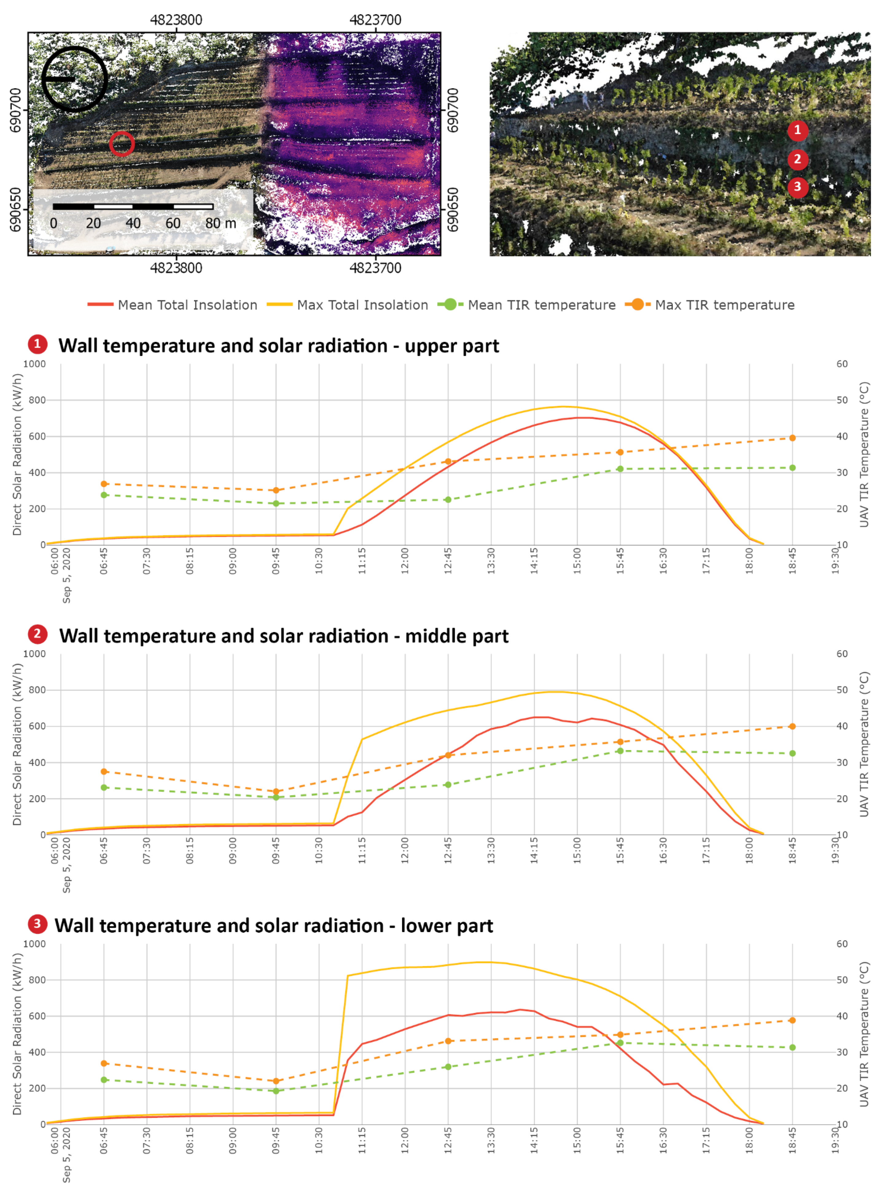
3.3.3. Feature Scale

The developed method was used for evaluating the solar performance of the dry-stone walls. The methods developed for solar simulations aimed at features such as the dry-stone walls are well suited for vertical elements, but the translation of point clouds to geometric representations that are compatible with the selected tools poses a challenge. Methods of point cloud voxelisation, flexible tools for semantic segmentation and point cloud conversion to different mesh representations are not implemented in discipline-specific tools. The capability of voxel models to encode volumetric information can be exploited to construct irregular volumetric objects, such as vine plants. The interface between CVMs and geoscientific raster formats makes it possible to construct continuous terrain surfaces. This enabled the construction of a geometric model compatible with the selected solar simulation tool [43], thereby enabling it to overcome the limitation of the 2.5D simulation tools related to vertical surfaces. The outcome of this simulation is presented in Figure 4.

3.4. Composite Voxel Model (CVM))

The CVM of the terraced vineyards in Lamole encodes multiple datasets into a single multidimensional object. The integration of datasets generated with the aforementioned methods is possible because of the data integration process. A central component of the data integration method is the voxelisation of different geospatial datasets, which makes it possible to impose a shared, three-dimensional grid and encode different information into the individual cells of the CVM. Figure 5 illustrates the concept of the multidimensional CVM model where each voxel cell can be visualised in a three-dimensional space. Multiple datasets encoded in the higher dimensions and visualised with dedicated colour scales can be chosen interactively and explored in the three-dimensional viewer interface.

3.4.1. Territorial Scale

The integration of the territorial scale data enabled the comparison of local environmental performance metrics and the assignment of individual vineyards to representative classes. The LiDAR dataset was extended with GIS data and simulated solar performance. This was supplemented with basic terrain metrics, such as the aspect and slope, and aligned with the structure of the CVM. All data used in the presented study was aligned to a common 3D grid. In this way, information created at one scale, such as vineyard classification, can be matched with the data from other scales. Based on the GIS data, individual vineyards were identified in the territorial dataset. The different datasets described above were combined into one multidimensional dataset. This approach shares data structuring and computational tools applied for the data cube creation and processing and enables the application of ML algorithms implemented in the scikit-learn [40] python library. In Figure 6, an exemplary application of K-Mean clustering is presented, where all vineyards included in the dataset can be divided into a specified amount of clusters based on their simulated environmental metrics. The first row in Figure 6 shows the layers of information encoded in the CVM at the territorial scale, including RGB data, vineyard ID, slope, aspect and sunlight hours for summer and winter solstice and the equinoxes. In the second row of Figure 6, the exemplary outcomes of the clustering are visualised. In the third row, two exemplary locations are presented: the Castello vineyard and the Grospoli II vineyard. For both vineyards, a summary of data encoded in the CVM was generated in the form of a composite graph. The distribution of slope (bar chart), aspect (yellow, circular diagram) and sunlight hours at four days (orange dots) are presented in the graph. This method facilitates comparative analysis through the exploratory application of unsupervised computational tools and the graphical representation of environmental metrics as interactive graphs.

3.4.2. Site Scale

The photogrammetric TIR acquisitions produced varying amounts of points caused by differentiated lighting conditions over the day and small distances between plants and walls. Only the points which contained TIR temperature values for every acquisition were included in the further analysis and complemented with the results of solar radiation analysis. This combined dataset was used to produce the graphs presented in Figure 7. The acquired temperature data were compared with the simulated incoming solar radiation in 15-min intervals to understand the differences in daily temperature variation (DTV) in characteristic locations in the vineyard.
For each point in the voxel model, a neighbourhood can be selected for which the temperature and solar radiation statistics are automatically plotted as a graph. In Figure 8, three characteristic areas are presented. Those neighbourhoods have dimensions of 2 × 2 m and represent the characteristic locations in the vineyard. In the exposed location (point 1 in Figure 8), a consistent trend of temperature change is visible. This matches with the change in solar radiation with an exception from 06:00 to 08:30, where the vineyard does not receive direct sunlight. This temperature change can be explained by the growing ambient air temperature and the contribution of indirect solar radiation. In the second graph (point 2 in Figure 8), a location close to the tree-lined areas along the edge of the vineyard is presented. In the early hours, the temperature is comparably low due to the shadowing of the ground by adjacent vegetation. At 09:45, the temperature encoded in some of the voxel cells in this neighbourhood is substantially higher than the mean value. The same is true for solar radiation values, suggesting that the shadowing effect of the adjacent vegetation is gradually disappearing. Between the third and fourth acquisition, a temperature change of 2 °C is visible. However, this difference is smaller than the precision of the TIR sensor. After 12:45, the temperature drops in every other ground location; however, in this particular location, the ground temperature stays stable until at least 15:45, and in the last acquisition maximum, the ground temperature next to the adjacent vegetation is 4 °C higher than that in the fully exposed location. The third graph (point 3 in Figure 8) describes the ground between the vine rows, where the temperature does not rise beyond 40 °C. Between the first two acquisitions, no substantial temperature change can be observed, which corresponds with the low values of solar radiation. In the later hours, a significant difference between the mean and maximum values of both the temperature and solar radiation is noted due to the shadow cast by the vine plants on the ground throughout the day.

3.4.3. Feature Scale

The method presented in the previous subsection can also be used to analyse the dry-stone wall surface temperature dynamics. The CVM can be queried for point neighbourhoods on the vertical surface of the wall. In Figure 9, three parts of the dry-stone wall are marked with numbers. The thermal performance of the dry-stone walls can be seen in the graphs in Figure 9 by observing the change in the TIR measured temperature at different heights of the wall. The temperature of the dry-stone wall increases constantly throughout the survey in contrast to the ground temperature, which starts to decrease in the afternoon. The difference between the maximum and mean temperatures is recorded at 12:45 in all parts of the dry-stone wall. Temperature dynamics can be further explained by integrating simulated solar radiation into the CVM, given the high temporal resolution of the simulated solar radiation data. The CVM makes it possible to compare both metrics three-dimensionally and to identify the time when a selected location starts receiving solar radiation and the temperature is expected to rise.
Graph 1 in Figure 9 shows the relation between the acquired temperature and simulated incoming solar radiation at the bottom of the dry-stone wall. The start of the direct insolation shifts in comparison with that in Figure 8 by two and half hours, from 08:15 to 10:45, but the total values of the solar radiation grow very rapidly. The difference between the maximum and mean radiation value throughout the day is the highest at the bottom of the dry-stone wall, likely due to vine plants casting irregular shadows on the wall. The effect of rising damp from the soil through the stone porosities (elongated cavities with small internal diameters) of the walls may also be considered to explain different temperature values in the bottom area. The capillary force, which develops due to the combined effect of surface tension and adhesive forces between the water and stone, causes moisture to rise due to capillary action. The evaporation and condensation of the inner water may cause temperature variations on the wall surface [47]. The middle part of the wall is described in Graph 2. Insolation starts at the same time as in Graph 1, but in the first 30 min, the mean value is low in comparison with that at the bottom of the wall. The curve describing mean radiation has an irregular shape, indicating radiation variations caused by shadowing. Graph 3 describes the topmost part of the wall; the amount of radiation grows slowly but very regularly. This is true for both maximum and mean values and could be explained by the lack of shadowing effects. After 16:30, the mean and maximum radiation values reach the same level, indicating that the upper part is constantly receiving substantial amounts of solar radiation. The observed trends reveal specific solar performance characteristics and temperature distributions in the vertical direction of the dry-stone walls.

3.4.4. Structure of the Composite Voxel Model (CVM)

In the previous subsections, the application of the CVM is described concerning three different scales. This is done on the example of a combined multi-scalar dataset. The implementation of the CVM commences with the input of point cloud data. Photogrammetric acquisitions in both RGB and TIR ranges were used to construct time series data. Geo-referenced point clouds collected with the UAV platform equipped with a dual sensor were grouped based on the acquisition time and voxelised to create a structure containing multi-temporal data. The LiDAR data was also voxelised and aligned with the structure of the voxel model. From the combined geometric structure of the voxel, a composite DSM, having the resolution of the photogrammetric data, was generated, incorporating surrounding tree canopy data from the airborne LiDAR dataset. Such a DSM model is a prerequisite to run the SAGA GIS potential incoming solar radiation analysis, which provides values of solar radiation at high resolution. The results of the incoming solar radiation simulation were fed back to the corresponding voxel cells for use in 3D visualisation and to produce quantitative outcomes automatically visualised as graphs. Analogous simulation at the scale of dry-stone walls and single plants is possible because of different geometric representations of voxel cells available within the CVM. A fully three-dimensional mesh-based representation of the CVM can be used with architectural tools for the simulation of solar radiation. The consistent application of a shared spatial grid makes it possible to feed the simulation results back to the CVM. Two methods of selecting point neighbourhoods are implemented. The first method allows the user to select a group of points contained within an area or volume centred on a manually selected location. Such point neighbourhoods contain an equally sized group of points and were used to generate the graphs that represent characteristic locations in the vineyard. The second method utilises scikit-learn k-d tree implementation [40] for the nearest neighbour search. For each point in the voxel, multiple neighbourhoods based on different neighbour point counts are generated. Geometric features are calculated for each neighbourhood size and used with the K-Means clustering algorithm. This method based on multi-scalar geometric features is commonly implemented for point cloud semantic segmentation [48,49]. In this study, multi-scalar geometric features were used in conjunction with the K-Means clustering algorithm, following the geo3dfeatures implementation [50] to generate semantic information describing individual objects contained in the CVM. Semantic segmentation can be run on arbitrary subsets of the dataset, allowing users to determine the number of classes and additional voxel cell parameters used in the segmentation. The same voxel cell parameters describing environmental performance can be evaluated quantitatively with basic statistical metrics displayed in graphs. This combination of user decision-driven semantic information describing singular objects linked with their performance parameters represents spatial knowledge that can be encoded back into the CVM. The structure of the proposed CVM is open-ended, allowing for future extensions with additional datasets, as well as methods that modify the structure and information content of the voxel. Figure 10 presents a workflow diagram describing the steps needed to construct the presented CVM.

4. Discussion

4.1. Development of the Composite Voxel Models (CVMs) through Further Surveys

The inclusion of the time dimension in the CVM brings benefits for studies at different scales. At the territorial scale, land use change and the resulting change of environmental conditions in the Lamole valley can be studied. At the scale of individual vineyards, past, present and future landforms and their environmental implications can be studied. At the feature scale, the presented methods could be applied for deformation monitoring of dry-stone walls for early identification of at-risk locations, surface runoff and mitigation of potential hydrological risks. Understanding the microclimatic impact of the green perimeter of the terraced vineyards that are frequently characterised by natural terrain features and vegetation requires studying at the territorial, site and feature scales, thereby necessitating multi-scale data integration. Our next survey will focus on these green perimeters. In this study, measured TIR data was correlated with the outcomes of solar exposure simulations. Trends related to the change in these parameters on the survey day are consistent, but the method to translate the solar radiation to the surface temperature of the dry-stone walls is still unresolved. Understanding the thermodynamic functioning of the dry-stone wall regarding the cooling effect of wind and thermal energy exchange with the ground and surrounding air poses a challenge. The application of multi-physics simulation methods, such as ANSYS FLUENT can explain the thermodynamic performance of the walls at the feature scale. This method has already been used for simulating relations between thermal mass and convection incorporating material-specific solar performance metrics at different scales.
Local growing conditions can be more comprehensively evaluated by combining information on the environmental conditions with quantitative insights related to the vine plants. Remote sensing methods are often applied in the context of precision agriculture using different platforms and sensors. Future work will investigate the integration of remotely and proximal sensed data to further increase spatial and temporal resolutions for studying daily temperature variations at the site and feature scales. The reliability and accuracy of low-cost non-radiometric TIR sensors for UAV-based surveys will be addressed based on a tailored sensor control network. Moreover, future experimental investigations will focus on the physicochemical characteristics of plants and their phenology to quantify the effect of microclimate on the grapevines. The combination with new UAV platforms, equipped with multi-spectral and radiometric thermal sensors, will also provide vegetation indexes to assess plant health and needs.

4.2. General Development of Composite Voxel Models (CVMs) and Related Workflows

The resolution of the collected data and the presented methods are limited at the feature scale. Further investigations are needed to advance the methods of point cloud processing and voxelisation to bridge different disciplinary contributions aimed at evaluating the environmental performance with the use of CVMs. Furthermore, efficient methods for the generation of different voxel model mesh representations are needed to include analysis and simulation tools for mesh-based representations.
As mentioned above, CVMs enable the integration and correlation of remote sensing data and processing methods with data obtained from geoscientific simulation tools. This implies the possibility of integrating multi-domain and multi-scale data, as well as correlating different datasets that are not easily comparable because of misaligned or non-interoperable methods and tools. CVMs can enable fully three-dimensional geometry and advanced computational methods, applied in the context of data-driven design. The introduction of additional spectral bands, such as NIR, can further extend the use of this method. Structured multi-spectral voxel models can be combined with ML algorithms to predict the values of TIR and NIR bands for the time periods between acquisitions and increase the temporal resolution.
Conventionally, there is a progression from acquired data through structured data processing and systematic storage of geospatial datasets. Subsequently, information is generated with geoscientific analysis and simulation tools and stored in specialised databases. The developed CVM combines existing methods and tools to form a continuous workflow in which spatial knowledge can be accumulated over time (Figure 11). The requirement to rapidly visualise multiple parameters encoded in the voxel cells, such as TIR temperature time series and simulated solar metrics, introduced an interactive 3D viewer interface linked with the voxel model. The possibility to create feedback loops related to analysis outcomes and geometric changes resulting from design decisions will be further developed in a follow-up study. The application of this information for decision support, i.e., adapting agricultural systems to different conditions or locations, requires dedicated methods and interfaces that often separate this process from previous steps.

4.3. The Bigger Picture: Decision Support for Land Knowledge Utilization

Land knowledge recovery is useful for maintenance and adaptation of productive landscape and also for adaptation and transfer of such knowledge for use in different context, such as cities, etc. This ultimately requires knowledge recovery across a broad range of cases. We commenced our research with a particular case of terraced landscapes. The latter are one of the many unique traditional agricultural systems shaped by human intervention that combines ingenuity in the construction and cultivation of land with the conservation of biodiversity and natural resources. Such systems can provide valuable insights for transitioning from resource-intensive to sustainable farming and land use. We have witnessed instances of solutions evolved and accumulated over time through experiential trial-and-error, and traditions passed down through generations, combined with local ecological knowledge. Such systems are invaluable repositories of land knowledge. The latter is critical but challenging to preserve, recover and adapt. Preservation is challenged by industrialisation, urbanisation and climate change. Required knowledge, skill and labour may now be rethought in the light of technological advancements, such as automation, robotics and sensor technologies [51]. Recovery is not a trivial task as such systems are complex, often not well documented and not always easily accessible. Furthermore, the solutions found in history are particular responses to environmental circumstances, needs and time constraints and therefore are difficult to assess in today’s circumstances. Their study demands interdisciplinary and transdisciplinary expertise involving a range of scientific disciplines and local practitioners, including farmers. From a design perspective, adaptation concerns the modification of constructions and practices as part of a resilience strategy to maintain and improve productivity in a changing environmental, land use and technological context. In addition, adaptation may involve utilising ideas gleaned from the past to better understand contemporary challenges as well as solving new problems through learning and history-inspired innovation (i.e., applying knowledge gained from the studies of rural designs to develop novel solutions for urban agriculture). Preservation, recovery and adaptation of land knowledge, including discovery, all rely on data, and modelling and analytical approaches have to balance simplification and critical resolution of complexity that characterise such systems.
Our ability to recover knowledge related to socio-ecological systems and environments that emerged from human–nature interaction over time is facilitated by data acquisition through remote sensing, GIS and other digital technologies. These technologies have a considerable impact on our ability to acquire, manage and analyse data. This progress helped to improve the outcomes of studies which challenge deep-seated preconceptions about the urban core and rural periphery and subsistence and intensive farming, as illustrated in the case of the ancient Maya agricultural terrace systems [52,53]. Further, the transfer of knowledge between the scientific and farming communities has helped dynamic conservation to safeguard time-tested agricultural heritage and livelihoods and provide practical guidelines for the future of rural development [54]. Vital information, which is necessary for informed decisions on the conservation, design, construction, management, planning and policy levels, can come from different sources, including archaeology, architecture, engineering, horticulture/agriculture and ecology.
Computational multi-criteria decision support systems (DSS) can play a key role in supporting adaptation and utilization of land knowledge. Multi-criteria decision methods (MCDM) entail identification of feasible key solutions to given problems. DSS can be model- or data-based, and its main components are databases, a DSS software system and a user interface. They serve to collect and analyse data to identify solutions and can be entirely computerized or operated by humans. At any rate, DSS can deliver a vital resource for tackling the involved complexity and large datasets derived from surveys, simulations and analyses. [55] While agricultural decision support systems exist, especially in the areas of precision and automated farming [56,57,58,59], there is a lack of systems tailored for adaptation. In this context, adaptation is considered both in terms of supporting the continuous adjustment of a system in response to change, as well as the transfer of knowledge to new contexts. Decision support is especially important in cases where decisions are based on traditional and local knowledge or a systematic framework is needed to make land knowledge accessible for adaptability to changing environments and different optimisation objectives and contexts. In this context, transdisciplinary research and a substantial amount of interviews with experts must complement data acquisition and analysis to capture aspects of practical knowledge that cannot be obtained through other means.
This article offers a necessary step in this direction using a particular voxel-based approach to storing, structuring and representing geo-referenced spatio-temporal data and heterogeneous datasets from different domains of study, whether derived from surveys or simulations and spanning from territorial to site and feature scales. The intention was to facilitate interoperability between planning and design methods, in particular through the connection of GIS with computer-aided design (CAD), thereby addressing issues related to resolution and three-dimensional accuracy. A follow-up study will integrate data coming from expert databases (that structure interdisciplinary datasets and analysis-derived information), databases (that structure local data from surveys and obtained from GIS) and optimisation (iterative optimisation of CAD models through simulation feedback) via computational ontologies tailored to facilitate the query, generation and manipulation of voxel models. The task of modelling agricultural terraced systems is the third step, after data acquisition and structuring, towards realising decision support for adaptation. We still need to address (1) the adaptation of any particular agricultural terraced system to support local farmers and (2) the adaptation of agricultural terraced system knowledge to the design and planning of urban agricultural systems [60]. The question is can the model be general enough to be applied to different agricultural terraced systems and yet be specific enough to respond locally? Therefore, the area which deserves particular attention is the systematic framework implemented for system analysis and modelling.

5. Conclusions

The primary goal of this article was to present a data-integration approach based on the use of a composite voxel model. To make this approach tangible, we discussed this approach with a focus on the thermal performance analysis of high-altitude terraced vineyards in Lamole, Tuscany, Italy. This was done with the aim of demonstrating how a multi-scale analysis can be facilitated. We summarised recent research on methods of data integration, correlation and acquisition concerning state-of-the-art remote sensing datasets combined with computational simulation tools. We demonstrated the environmental performance analysis of high-altitude terraced vineyards in Lamole, Tuscany, on three correlated spatial scales. Further, we developed a CVM to effectively generate, store and combine spatial information by combining the data of RGB and TIR photogrammetric acquisitions of the terraced vineyards. A deeper understanding of the environmental performance is required for combining measured parameters with geospatial simulations. The utilisation of open-access GIS and large-scale airborne LiDAR data provided new insights into extracting the environmental performance of individual vineyards in similar locations in the Lamole valley. Geometric and temperature data from the photogrammetric acquisition was supplemented with simulations of solar irradiance. Our approach allowed us to encode interdisciplinary knowledge into a combined geo-referenced dataset. Based on our research, we seek to develop a decision support system for broadly adapting agricultural systems, such as high-altitude terraced vineyards, to different conditions and contexts.

Supplementary Materials

The following are available online at https://www.mdpi.com/article/10.3390/rs13173483/s1, Figure S1: Workflow diagram presenting the steps needed to construct the CVM. Left: datasets used to construct the model. Right: interfaces with external simulation tools, as well as data processing and visualisation methods. Analysis and simulation results, such as incoming solar radiation, are fed back to the CVM, thereby creating feedback loops. This is as full page version of Figure 10 presented in the article, Figure S2: Workflows for generating spatial knowledge via (a) a conventional sequential approach and (b) the proposed composite voxel model (CVM)-based approach. This is as full page version of Figure 11 presented in the article.

Author Contributions

This work was conceptualised by J.T.; supervised by M.U.H. and D.S.H.; data was acquired by J.T., E.I.P. and M.U.H.; surveys were facilitated and supervised by G.T., E.I.P., D.S.H. and M.U.H.; data processing, visualisations and software integration were executed by J.T., D.S.H. and M.U.H. All authors have read and agreed to the published version of the manuscript.

Funding

This research received no external funding.

Data Availability Statement

Restrictions apply to the availability of these data. Data obtained from Servizi di Informazione Territoriale (S.I.T.) s.r.l. (https://www.sit-puglia.it/ accessed on 8 July 2021) as well as Servizio Idrologico Regionale (SIR) of the Tuscan Region (https://www.sir.toscana.it/ accessed on 8 July 2021) and are available from the authors with the permission of aforementioned institutions. GIS data is available as Open Data through Geoscopio Portal of Regione Toscana (https://www.regione.toscana.it/-/geoscopio accessed on 8 July 2021).

Acknowledgments

First and foremost, we wish to acknowledge Paolo Socci, proprietor of Fattoria di Lamole, whose long-term commitment and work in Lamole established the context for this research. The research collaboration commenced in 2016 involving the Geomatics for Environment and Conservation of Cultural Heritage Laboratory (GeCo) at the University of Florence and, in the first phase, the Research Centre for Architecture and Tectonics (RCAT) at the Oslo School of Architecture and Design (2016 to 2018) (Oslo, Norway). In the second phase, the Research Department for Digital Architecture and Planning (DAP) at Vienna University of Technology (2018-present) replaced RCAT. At the GeCo Lab, we wish to acknowledge Assistant Valentina Bonora, Associate Andrea Masiero, Assistant Francesco Mugnai, Brig. Gen. Enzo Santoro and Filippo Fiaschi for their contribution to the survey activities. The authors wish to thank the Servizi di Informazione Territoriale (S.I.T. s.r.l.) of Noci (Bari, Italy), especially technical director Nicola D’Elia and Air Operations Manager Ruggero Palumbo for providing the airborne territorial survey. Meteorological data were provided by Lorenzo Arcidiaco and Manuela Corongiu from LaMMA Consortium—Environmental Modelling and Monitoring Laboratory for Sustainable Development (Florence, Italy). At RCAT, we wish to acknowledge Associate Søren Sørensen, Assistant Professors Sofia Cunha and Joakim Wiig Hoen and Sareh Saeidi. At DAP, we wish to acknowledge senior lecturers Sigrun Swoboda, Arnold Faller and Andreas Jonas, as well as Bianca Braun. Open Access Funding by TU Wien. The authors acknowledge the Library at Vienna University of Technology for financial support through its open-access funding programme.

Conflicts of Interest

The authors declare no conflict of interest.

References

  1. Pretty, J. Interdisciplinary progress in approaches to address social-ecological and ecocultural systems. Environ. Conserv. 2011, 38, 127–139. [Google Scholar] [CrossRef] [Green Version]
  2. Sunderland, T.; Abdoulaye, R.; Ahammad, R.; Asaha, S.; Baudron, F.; Deakin, E.; Duriaux, J.-Y.; Eddy, I.; Foli, S.; Gumbo, D.; et al. A methodological approach for assessing cross-site landscape change: Understanding socio-ecological systems. For. Policy Econ. 2017, 84, 83–91. [Google Scholar] [CrossRef]
  3. Zscheischler, J.; Rogga, S.; Busse, M. The adoption and implementation of transdisciplinary research in the field of land-use science—A comparative case study. Sustainability 2017, 9, 1926. [Google Scholar] [CrossRef] [Green Version]
  4. UNESCO. Intergovernmental Committee for the Safeguarding of the Intangible Cultural Heritage Decision of the Intergovernmental Committee: 13.COM 10.B.10 2018. Available online: https://ich.unesco.org/en/decisions/13.COM/10.B.10 (accessed on 15 July 2021).
  5. FAO. GIHAS, Globally Important Agricultural Heritage Systems. Available online: http://www.fao.org/giahs/background/a-global-partnership/en/ (accessed on 3 January 2021).
  6. Varotto, M.; Bonardi, L.; Tarolli, P. World Terraced Landscapes: History, Environment, Quality of Life; Springer: Cham, Switzerland, 2019; ISBN 978-3-319-96815-5. [Google Scholar]
  7. Agnoletti, M.; Conti, L.; Frezza, L.; Monti, M.; Santoro, A. Features analysis of dry stone walls of Tuscany (Italy). Sustainability 2015, 7, 13887–13903. [Google Scholar] [CrossRef] [Green Version]
  8. Agnoletti, M.; Conti, L.; Frezza, L.; Santoro, A. Territorial analysis of the agricultural terraced landscapes of Tuscany (Italy): Preliminary Results. Sustainability 2015, 7, 4564–4581. [Google Scholar] [CrossRef] [Green Version]
  9. Spanò, A.; Sammartano, G.; Tunin, F.C.; Cerise, S.; Possi, G. GIS-based detection of terraced landscape heritage: Comparative tests using regional DEMs and UAV data. Appl. Geomat. 2018, 10, 77–97. [Google Scholar] [CrossRef] [Green Version]
  10. Stubert, L.; Martín i Oliveras, A.; Märker, M.; Schernthanner, H.; Vogel, S. Viticulture in the Laetanian Region (Spain) during the Roman Period: Predictive modelling and geomatic analysis. Geosciences 2020, 10, 206. [Google Scholar] [CrossRef]
  11. Tarolli, P.; Preti, F.; Romano, N. Terraced landscapes: From an old best practice to a potential hazard for soil degradation due to land abandonment. Anthropocene 2014, 6, 10–25. [Google Scholar] [CrossRef]
  12. Agnoletti, M.; Errico, A.; Santoro, A.; Dani, A.; Preti, F. Terraced landscapes and hydrogeological risk. Effects of land abandonment in Cinque Terre (Italy) during severe rainfall events. Sustainability 2019, 11, 235. [Google Scholar] [CrossRef] [Green Version]
  13. Preti, F.; Tarolli, P.; Dani, A.; Calligaro, S.; Prosdocimi, M. LiDAR derived high resolution topography: The next challenge for the analysis of terraces stability and vineyard soil erosion. J. Agric. Eng. 2013, 44. [Google Scholar] [CrossRef]
  14. Preti, F.; Guastini, E.; Penna, D.; Dani, A.; Cassiani, G.; Boaga, J.; Deiana, R.; Romano, N.; Nasta, P.; Palladino, M.; et al. Conceptualization of water flow pathways in agricultural terraced landscapes. Land Degrad. Dev. 2018, 29, 651–662. [Google Scholar] [CrossRef]
  15. Tarolli, P.; Sofia, G.; Calligaro, S.; Prosdocimi, M.; Preti, F.; Dalla Fontana, G. Vineyards in terraced landscapes: New opportunities from Lidar Data. Land Degrad. Dev. 2015, 26, 92–102. [Google Scholar] [CrossRef]
  16. Pijl, A.; Reuter, L.E.H.; Quarella, E.; Vogel, T.A.; Tarolli, P. GIS-based soil erosion modelling under various steep-slope vineyard practices. Catena 2020, 193, 104604. [Google Scholar] [CrossRef]
  17. Pijl, A.; Quarella, E.; Vogel, T.A.; D’Agostino, V.; Tarolli, P. Remote sensing vs. field-based monitoring of agricultural terrace degradation. Int. Soil Water Conserv. Res. 2021, 9, 1–10. [Google Scholar] [CrossRef]
  18. Preti, F.; Errico, A.; Caruso, M.; Dani, A.; Guatsini, E. Dry-stone wall terrace monitoring and modelling. Land Degrad. Dev. 2018, 29, 1806–1818. [Google Scholar] [CrossRef]
  19. Hensel, M.; Sunguroğlu Hensel, D.; Sørensen, S.S. Embedded Architectures: Inquiries into architectures, diffuse heritage and natural environments in search for better informed design approaches to sustainability. Time Archit. 2018, 3, 42–45. [Google Scholar]
  20. Tucci, G.; Parisi, E.I.; Castelli, G.; Errico, A.; Corongiu, M.; Sona, G.; Viviani, E.; Bresci, E.; Preti, F. Multi-sensor UAV application for thermal analysis on a dry-stone terraced vineyard in rural Tuscany landscape. Int. J. Geo-Inf. 2019, 8, 87. [Google Scholar] [CrossRef] [Green Version]
  21. Parisi, E.; Suma, M.; Korumaz, A.G.; Rosina, E.; Tucci, G. Aerial Platforms (UAV) Surveys in the VIS and TIR range. Applications on archaeology and agriculture. Int. Arch. Photogramm. Remote. Sens. Spat. Inf. 2019, XLII-2/W11, 945–952. [Google Scholar] [CrossRef] [Green Version]
  22. Parisi, E.I.; Tyc, J. Multi-scale and multi-domain approaches for cultural terraced landscapes. In Proceedings of the ARQUEOLÓGICA 2.0—9th International Congress & 3rd GEORES—GEOmatics and pREServation, Editorial Universitat Politècnica de València, València, Spain, 26 April 2021; pp. 317–324. [Google Scholar] [CrossRef]
  23. Rupnik, E.; Daakir, M.; Pierrot Deseilligny, M. MicMac–a free, open-source solution for photogrammetry. Open Geospat. Data Softw. Stand. 2017, 2, 14. [Google Scholar] [CrossRef]
  24. Schönberger, J.L.; Frahm, J. Structure-from-motion revisited. In Proceedings of the 2016 IEEE Conference on Computer Vision and Pattern Recognition (CVPR), Las Vegas, NV, USA, 27–30 June 2016; pp. 4104–4113. [Google Scholar] [CrossRef]
  25. Schönberger, J.L.; Price, T.; Sattler, T.; Frahm, J.-M.; Pollefeys, M. A Vote-and-Verify Strategy for Fast Spatial Verification in Image Retrieval. In Computer Vision—ACCV 2016. Lecture Notes in Computer Science; Lai, S.H., Lepetit, V., Nishino, K., Sato, Y., Eds.; Springer: Cham, Switzerland, 2017; pp. 321–337. ISBN 978-3-319-54180-8. [Google Scholar]
  26. Kelly, J.; Kljun, N.; Olsson, P.-O.; Mihai, L.; Liljeblad, B.; Weslien, P.; Klemedtsson, L.; Eklundh, L. Challenges and best practices for deriving temperature data from an uncalibrated UAV thermal infrared camera. Remote Sens. 2019, 11, 567. [Google Scholar] [CrossRef] [Green Version]
  27. Tang, H.; Swatantran, A.; Barrett, T.; DeCola, P.; Dubayah, R. Voxel-based spatial filtering method for canopy height retrieval from airborne single-photon Lidar. Remote Sens. 2016, 8, 771. [Google Scholar] [CrossRef] [Green Version]
  28. Brolly, G.; Király, G.; Lehtomäki, M.; Liang, X. Voxel-based automatic tree detection and parameter retrieval from terrestrial laser scans for plot-wise forest inventory. Remote Sens. 2021, 13, 542. [Google Scholar] [CrossRef]
  29. Li, S.; Dai, L.; Wang, H.; Wang, Y.; He, Z.; Lin, S. Estimating leaf area density of individual trees using the point cloud segmentation of terrestrial LiDAR Data and a voxel-based model. Remote Sens. 2017, 9, 1202. [Google Scholar] [CrossRef] [Green Version]
  30. Consortium Project Pantheon Project—Supervisory Control and Data Acquisition (SCADA) System for the Precision Farming of Hazelnut Orchards. Available online: http://pantheon.inf.uniroma3.it/ (accessed on 19 March 2021).
  31. Lamprecht, S. Pyoints: A Python package for point cloud, voxel and raster processing. J. Open Source Softw. 2019, 4, 990. [Google Scholar] [CrossRef]
  32. Carpio, R.F.; Potena, C.; Maiolini, J.; Ulivi, G.; Rosselló, N.B.; Garone, E.; Gasparri, A. A navigation architecture for Ackermann vehicles in precision farming. IEEE Robot. Autom. Lett. 2020, 5, 1103–1110. [Google Scholar] [CrossRef]
  33. Jurado, J.M.; Ortega, L.; Cubillas, J.J.; Feito, F.R. Multispectral mapping on 3D models and multi-temporal monitoring for individual characterization of olive trees. Remote Sens. 2020, 12, 1106. [Google Scholar] [CrossRef] [Green Version]
  34. QGIS Geographic Information System. Open Source Geospatial Foundation Project. 2021. Available online: http://qgis.org (accessed on 15 July 2021).
  35. Conrad, O.; Bechtel, B.; Bock, M.; Dietrich, H.; Fischer, E.; Gerlitz, L.; Wehberg, J.; Wichmann, V.; Böhner, J. System for Automated Geoscientific Analyses (SAGA) v. 2.1.4. Geosci. Model Dev. 2015, 8, 1991–2007. [Google Scholar] [CrossRef] [Green Version]
  36. Zhao, Q.; Wentz, E.A. A MODIS/ASTER airborne simulator (MASTER) imagery for urban heat island research. Data 2016, 1, 7. [Google Scholar] [CrossRef] [Green Version]
  37. Kopp, S.; Becker, P.; Doshi, A.; Wright, D.J.; Zhang, K.; Xu, H. Achieving the full vision of earth observation data cubes. Data 2019, 4, 94. [Google Scholar] [CrossRef] [Green Version]
  38. Dask: Scalable analytics in Python. Anaconda Inc. and Contributors. 2021. Available online: https://dask.org (accessed on 15 July 2021).
  39. Hoyer, S.; Hamman, J. Xarray: N-D labeled arrays and datasets in Python. J. Open Res. Softw. 2017, 5, 10. [Google Scholar] [CrossRef] [Green Version]
  40. Pedregosa, F.; Varoquaux, G.; Gramfort, A.; Michel, V.; Thirion, B.; Grisel, O.; Blondel, M.; Prettenhofer, P.; Weiss, R.; Dubourg, V.; et al. Scikit-Learn: Machine Learning in Python. J. Mach. Learn. Res. 2011, 12, 2825–2830. [Google Scholar]
  41. Toja-Silva, F.; Lopez-Garcia, O.; Peralta, C.; Navarro, J.; Cruz, I. An empirical–heuristic optimization of the building-roof geometry for urban wind energy exploitation on high-rise buildings. Appl. Energy 2016, 164, 769–794. [Google Scholar] [CrossRef]
  42. Vuorinen, V.; Chaudhari, A.; Keskinen, J.-P. Large-eddy simulation in a complex hill terrain enabled by a compact fractional step OpenFOAM® solver. Adv. Eng. Softw. 2015, 79, 70–80. [Google Scholar] [CrossRef]
  43. Roudsari, M.S.; Pak, M.; Smith, A.; Gill, G. Ladybug: A parametric environmental plugin for grasshopper to help designers create an environmentally-conscious design. In Proceedings of the 13th Conference of International Building Performance Simulation Association (BS2013), Chambery, France, 26 August 2013; pp. 3128–3135. [Google Scholar]
  44. Böhner, J.; Antonić, O. Chapter 8 Land-surface parameters specific to topo-climatology. Dev. Soil Sci. 2009, 33, 195–226. [Google Scholar] [CrossRef]
  45. Wilson, J.P.; Gallant, J.C. Secondary topographic attributes. In Terrain Analysis: Principles and Applications; Wilson, J.P., Gallant, J.C., Eds.; John Wiley and Sons: New York, NY, USA; pp. 87–131. ISBN 978-0-471-32188-0.
  46. Hofierka, J.; Suri, M. The solar radiation model for open source GIS: Implementation and applications. In Proceedings of the Open Source GIS-GRASS Users Conference, Trento, Italy, 11–13 September 2002; pp. 51–70. [Google Scholar]
  47. Massari, G.; Massari, I. Damp buildings, old and new. Bull. Assoc. Preserv. Technol. 1985, 17, 2–30. [Google Scholar] [CrossRef]
  48. Brodu, N.; Lague, D. 3D terrestrial LiDAR data classification of complex natural scenes using a multi-scale dimensionality criterion: Applications in geomorphology. ISPRS J. Photogramm. Remote. Sens. 2012, 68, 121–134. [Google Scholar] [CrossRef] [Green Version]
  49. Weinmann, M.; Jutzi, B.; Hinz, S.; Mallet, C. Semantic point cloud interpretation based on optimal neighborhoods, relevant features and efficient classifiers. ISPRS J. Photogramm. Remote. Sens. 2015, 105, 286–304. [Google Scholar] [CrossRef]
  50. Raphaël Delhome; Damien Garaud; Romain Leroux-Mallouf geo3dfeatures. 2021. Available online: https://gitlab.com/Oslandia/geo3dfeatures/ (accessed on 12 July 2021).
  51. Bürgi, M.; Bieling, C.; von Hackwitz, K.; Kizos, T.; Lieskovský, J.; Martín, M.G.; McCarthy, S.; Müller, M.; Palang, H.; Plieninger, T.; et al. Processes and driving forces in changing cultural landscapes across Europe. Landsc. Ecol. 2017, 32, 2097–2112. [Google Scholar] [CrossRef] [Green Version]
  52. Chase, A.F.; Chase, D.Z.; Weishampel, J.F.; Drake, J.B.; Shrestha, R.L.; Slatton, K.C.; Awe, J.J.; Carter, W.E. Airborne LiDAR, archaeology, and the ancient Maya landscape at Caracol, Belize. J. Archaeol. Sci. 2011, 38, 387–398. [Google Scholar] [CrossRef]
  53. Chase, A.F.; Chase, D.Z. Scale and intensity in classic period Maya agriculture: Terracing and settlement at the ‘Garden City’ of Caracol, Belize. Cult. Agric. 1998, 20, 60–77. [Google Scholar] [CrossRef]
  54. Koohafkan, P.; Altieri, M. Forgotten Agricultural Heritage: Reconnecting Food Systems and Sustainable Development; Routledge: Milton Park, UK, 2016; ISBN 9781138204157. [Google Scholar]
  55. Sprague, R.H., Jr. A Framework for the Development of Decision Support Systems. MIS Q. 1980, 4, 1–26. [Google Scholar] [CrossRef]
  56. Perini, A.; Susi, A. Developing a decision support system for integrated production in agriculture. Environ. Model. Softw. 2004, 19, 821–829. [Google Scholar] [CrossRef]
  57. Rose, D.C.; Sutherland, W.J.; Parker, C.; Lobley, M.; Winter, M.; Morris, C.; Twining, S.; Ffoulkes, C.; Amano, T.; Dicks, L.V. Decision support tools for agriculture: Towards effective design and delivery. Agric. Syst. 2016, 149, 165–174. [Google Scholar] [CrossRef] [Green Version]
  58. Zhai, Z.; Martínez, J.F.; Beltran, V.; Martínez, N.L. Decision support systems for agriculture 4.0: Survey and challenges. Comput. Electron. Agric. 2020, 170, 105256. [Google Scholar] [CrossRef]
  59. Castrignano, A.; Buttafuoco, G.; Khosla, R.; Mouazen, A.; Moshou, D.; Naud, O. Agricultural Internet of Things and Decision Support. for Precision Smart Farming, 1st ed.; Academic Press-Elsevier: Cambridge, MA, USA, 2020; ISBN 9780128183731. [Google Scholar]
  60. Sunguroğlu Hensel, D. Ecological Prototypes: Initiating design innovation in Green Construction. Sustainability 2020, 12, 5865. [Google Scholar] [CrossRef]
Figure 1. Understanding the interactions between terraced vineyards and their environments requires multi-scale methods. In this study, thermal performance was investigated at three distinct scales: the territorial scale (a), the site scale, i.e., individual vineyard (b), and the feature scale, i.e., dry-stone walls or plants (c). Investigations at each scale were spatially matched, and the same methods and tools were used for each scale to enable correlation of the outcomes.
Remotesensing 13 03483 g001
Figure 2. (a) Graph illustrating the comparison between the outcomes of the SAGA GIS potential incoming solar radiation analysis of an exposed location in Grospoli II vineyard (marked with red, continuous line) and global horizontal irradiance (GHI) measured by the local meteorological station in Lamole (marked with orange, dashed line). (b) Map illustrating the chosen location in Grospoli II vineyard (marked in red) and the exact location of the local meteorological station in Lamole (marked in orange).
Remotesensing 13 03483 g002
Figure 3. (a) Outcomes of the potential incoming solar radiation simulation from SAGA GIS at 16:00 during the summer solstice, computed with LiDAR data. (b) The same simulation computed with photogrammetric data only. The limited resolution of LiDAR data does not show the dry-stone walls’ solar performance in the afternoon. Photogrammetric data exposes this trend, but the impact of the surrounding vegetation cannot be evaluated. Only by merging those two datasets in different scales do we obtain a more complete picture of the dry-stone walls’ solar performance.
Remotesensing 13 03483 g003
Figure 4. Fully three-dimensional solar radiation simulation performed in the Grasshopper plug-in Ladybug Tools [43]. The values of the total solar radiation were collected from the local meteorological station. (a) Representative fragment of the vineyard was chosen. (b) Custom mesh representations of the CVM was constructed in Grasshopper. (c) The outcomes of the analysis for the ground cells were fed back to the CVM.
Remotesensing 13 03483 g004
Figure 5. Different layers of spatial information encoded into the CVM of the terraced vineyards in Lamole. For each voxel cell, geometric and RGB values, thermal infrared (TIR) temperature data and the simulated solar radiation were encoded. These datasets can be interactively displayed in the multidimensional viewer interface.
Remotesensing 13 03483 g005
Figure 6. Exemplary application of K-Means clustering to identify vineyards that share similar environmental performance metrics. Each location marked as a vineyard in open-access GIS data is included and can be queried in the CVM. Summary statistics are automatically generated for any vineyard in the dataset for comparison.
Remotesensing 13 03483 g006
Figure 7. Images of a photogrammetric voxel model that encodes both geometric data and surface temperature measured during the UAV TIR acquisition. The resolution of this dataset allows for investigations at the feature scale, addressing relations between dry-stone walls and plants. The amount of captured points varies in the time series, depending on the quality of a single photogrammetric acquisition. The photogrammetric dataset presented here was used to construct the digital surface model and conduct incoming solar radiation analysis. In the bottom row, exemplary outcomes of the radiation analysis in the morning (a) and late afternoon (b) are presented.
Remotesensing 13 03483 g007
Figure 8. Top view of the voxel model with characteristic locations in the vineyard marked with numbers: (1) The ground in a strongly exposed location, (2) close to the edge of the forest and (3) in between the vine rows. The corresponding graphs on the left show measured daily temperature variation (DTV) compared with simulated solar exposure.
Remotesensing 13 03483 g008
Figure 9. Graphs show the relation between daily temperature variation (DTV) and simulated solar radiation of a dry-stone wall. In the top view of the voxel model, red circle marks the exact location in the vineyard where the samples for the graphs were taken. Three-dimensional view of this location shows parts of the dry-stone wall chosen for the comparison marked with numbers.
Remotesensing 13 03483 g009
Figure 10. Workflow diagram presenting the steps needed to construct the CVM. Left: datasets used to construct the model. Right: interfaces with external simulation tools, as well as data processing and visualisation methods. Analysis and simulation results, such as incoming solar radiation, are fed back to the CVM, thereby creating feedback loops. This figure is available in Supplementary Materials (Figure S1) as a high-resolution, full page illustration.
Remotesensing 13 03483 g010
Figure 11. Workflows for generating spatial knowledge via (a) a conventional sequential approach and (b) the proposed composite voxel model (CVM)-based approach. This figure is available in Supplementary Materials (Figure S2) as a high-resolution, full page illustration.
Remotesensing 13 03483 g011
Table 1. Key parameters describing datasets used in this study. The spatial resolution was reported as ground sample distance (GSD) for RGB photogrammetry and LiDAR, and instantaneous field of view for TIR data.
Photogrammetry
RGB
Photogrammetry
TIR
Airborne
LiDAR
Spatial Resolution2 cm GSD4 cm IFOV @ 60 m50 cm GSD
Time series5 acquisitions per day5 acquisitions per day-
Total number of pointsca. 215.000.000 points on average for 5 acquisitions 15.569.983 points
Total area covered Grospoli II vineyard—1.1 haLamole valley—341 ha
Available data productsunclassified RGB
point cloud
TIR temperature data encoded as a point cloud classified LiDAR point cloud, DSM, DTM
PlatformDJI Mavic 2 Enterprise DualVulcanair P68 B Victor
SensorsRGB: DJI M2ED 1/2.3″ CMOS; 12MP
TIR: FLIR Lepton 3.5 160 × 120 px
LiDAR: Riegl LMS-Q680i
Acquisition date5 September 20206 August 2020
Publisher’s Note: MDPI stays neutral with regard to jurisdictional claims in published maps and institutional affiliations.

