Abstract
Rain affects the wind measurement accuracy of the Ku-band spaceborne scatterometer. In order to improve the quality of the retrieved wind field, it is necessary to identify and flag rain-contaminated data. In this study, an HY-2A scatterometer is used to study rain identification. In addition to the conventional parameters, such as the retrieved wind speed, the wind direction relative to the along-track direction, and the normalized beam difference, the experiment expands the mean deviation of the backscattering coefficient, the beam difference between fore and aft, and the node number of the wind vector cell (WVC) as the sensitive parameters according to the microwave scattering characteristics of rain and the actual measurement situation of the HY-2A. Furthermore, a rain identification model for HY2 (HY2RRM) with the K-Nearest Neighborhood (KNN) algorithm was built. After several tests, the accuracy of the selected HY2RRM approach is found to about 88%, and about 70% of rain-contaminated data can be accurately identified. The research results are helpful for better understanding the characteristics of microwave backscattering and provide a possible way to further improve the wind field retrieval accuracy of the HY-2A scatterometer and other Ku-band scatterometers.
1. Introduction
The remote sensing of sea surface wind fields is an important branch of remote sensing applications that has been widely used in civil and military fields. As a result, the acquisition of sea surface wind field data at a high spatial and temporal resolution has very important scientific implications and practical significance. The advent of spaceborne scatterometers has provided a technology for obtaining real-time data of sea surface wind fields with high precision and spatio-temporal resolution [1]. Although scatterometers can work in all weather and at all times, the influence of rain on the scatterometer cannot be ignored; in particular, for a scatterometer in the Ku-band, this will cause the wind field measurement accuracy to decrease by 4–10% [2]. The mechanism of measuring wind with scatterometers is multi-azimuth measurement, and the different responses of surface roughness to radar backscattering coefficients under different wind speeds are used to indirectly obtain the sea surface wind field information. However, drops of rainfall attenuate and scatter the microwave signal, and the splashing of raindrops changes the roughness of the sea surface, which increases the variance of scatterometer measurements [3,4]. If the influence of rain is not considered in wind field retrieval, the contribution of raindrops will be interpreted as the characteristics of wind, reducing the quality of wind field retrieval. As a result, it is necessary to identify and process the rain-contaminated data when inverting a wind field. However, not all satellites are good at recognizing or measuring rain, such as the marine dynamic environment satellites, because of the different observation objects, payload designs, and antenna technologies of satellites. There are few studies on the rain identification abilities of marine dynamic environmental satellites.
The famous marine dynamic environment satellites of the past few decades include ASCAT and SeaWinds. Many domestic and foreign scholars have proposed some methods to eliminate the influence of rain for these two scatterometers, which can be summarized as follows: the first approach is to build a rain identification model by selecting several rain-sensitive parameters, such as brightness temperature, retrieved wind speed, normalized beam difference, etc., and then identify and flag the rain-contaminated data in retrieved wind field products. The most representative model is the multidimensional histogram rain-flagging technique (MUDH), which has been successfully applied to the SeaWinds scatterometer on QuickSat by JPL, creating a precedent for the scatterometer to identify rain [5]. When the algorithm was applied to the ADEOS-2 satellite, JPL improved it and renamed it to Rain-Impact Detection (IMUDH), mainly reducing the over-flagging of high wind speeds and the removal of swath artifacts including over-flagging in the outer swath [6,7]. The second method is to use the quality control flag to filter out rain-contaminated data. It is found that there is a good correlation between the quality control flag and rain flag, which has a certain reference value in judging whether there is rain [8,9,10]. The third strategy obtains information data by matching external data and then extends rain as an independent variable to the geophysical model function (GMF) so that the new GMF can also consider the influence of rain [11,12,13,14,15,16,17]. The fourth approach is to study the transmission process and scattering characteristics of microwaves on rainy days and then construct the microwave radiation transmission model under rainy conditions, which can correct the influence of rain on the wind measurement [18,19,20,21].
In contrast, there are few relevant research works on Chinese Marine dynamical environmental satellites. At present, the HY-2A still cannot identify rain-contaminated data by itself, which limits the scatterometer in terms of further improving the wind measurement accuracy. If the HY-2A data need to be corrected for rain influence, the rain information can only be obtained by matching ECMWF, SSM/I, NECP, and other external data. However, in the process of matching, the huge amount of data requires a great amount of time to process, and some WVCs often fail to match the data, resulting in a failure to obtain complete rainfall information. Besides, the processing has hysteresis, so the wind measured by the scatterometer cannot be corrected for rain influence in real-time. Consequently, the HY-2A must be able to identify rain-contaminated data independently.
This study refers to the MUDH technique and explores the response characteristics of the HY-2A satellite to rain to select some suitable rain-sensitive parameters to build a rainfall identification model (HY2RRM). Then, the performance of the HY2RRM and MUDH techniques transplanted to the HY-2A satellite is compared, and the difficulties encountered in using other satellite rainfall recognition models are discussed. The main contributions of this study include the following:
- (1)
- According to the actual measurement conditions of HY-2A, the study builds a rain identification model that preliminarily realizes the function of identifying rain-contaminated data;
- (2)
- The HY2RRM is simple and effective, easy to transplant, and can overcome some limitations of the traditional MUDH technique, such as the ability to calculate high-dimensional data, and is suitable for all WVCs;
- (3)
- The HY-2A scatterometer was firstly taken as the research object to study rain identification, and its product information is improved—it is our goal to further improve the wind measurement accuracy of HY-2A and improve its application level in oceanography, meteorology, and other fields.
The primary goal of this study is to control the quality of HY2A data better and provide people with high-quality sea surface wind field data. The rest of this paper is organized as follows: in Section 2, the data used in the experiment and the rain-sensitive parameters and KNN algorithm needed to build the rain identification model are introduced. Section 3 explores the response of the rain-sensitive parameters to rain and the performance of rain identification models under different standards; finally, the discussion and conclusions are presented in Section 4 and Section 5.
2. Data and Methods
In this study, the L2A and L2B data of the HY-2A scatterometer and ECMWF reanalysis wind field data were used to explore the response of the HY-2A scatterometer to rain to select the appropriate rain-sensitive parameters to build a rain identification model. The process can be divided into the following four steps:
- Step 1: The data were preprocessed before building the rain identification model, including spatiotemporal matching, outlier elimination, data classification, etc.
- Step 2: The influence of rainfall on each parameter was analyzed and compared, and then the more sensitive parameters were selected to establish the rain identification model.
- Step 3: The KNN method was used to build some rainfall identification models under different rainfall identification criteria. In addition, we also attempted to use the MUDH technology as a comparative experiment.
- Step 4: The performance of each model and the influence on the quality of the retrieved wind field were evaluated by using the confusion matrix, and then the most suitable HY2RRM was selected.
2.1. Data Sets
The data used in this study mainly included the measured backscattering coefficient data, sea surface wind field retrieval data, and sea surface precipitation data; these data were from 1 January 2013 to 30 June 2013.
Regarding the measured backscattering coefficient data, Level-2A data of HY-2A were used in the study, which was stored along the track in the HDF5 format. The L2A data contain 1702 × 76 WVCs, and each WVC contains measured backscattering coefficients from different azimuths and polarizations, as well as the corresponding observation time, longitude, latitude, incident angle, azimuth, etc.
Regarding the sea surface wind field retrieval data, level-2B data of HY-2A were used in this study, and the storage mode was consistent with that of L2A. Level-2B data use NSCAT2 and the maximum likelihood estimate (MLE) to invert the wind field from level-2A data and then filter the ambiguity using the circle median filter approach. Each WVC of the L2B data contains parameters such as the inversion wind speed and direction, observation time, longitude and latitude, etc.
Regarding sea-surface precipitation data, we adopted ECMWF reanalysis data, which use a relatively complete data assimilation system to reintegrate and optimize the observation data of various types and from various sources, and the products have been widely used in previous atmospheric research [22]. In addition, HY2A and ECMWF can match more data than other data, such as SSM-I. In this paper, 0.125° × 0.125° high-resolution ECMWF reanalysis data were used, with a time interval of 3 h.
2.2. Data Preprocessing
The most important part of data preprocessing is data spatio-temporal matching. When matching the ECMWF data with the L2A and L2B, adopting the L2A WVCs as the reference cells, the nearest point spatially and temporally to the ECMWF data was selected as the matching point with a spatial window of 0.125° and a temporal window of 0.5 h. After data matching, in order to reduce the impact of data error on the experiment, it was necessary to carry out quality control on the matched data. Firstly, data lacking L2B wind speed and direction or with a precipitation less than 0 mm/h were eliminated. Then, the wind direction of ECMWF was compared with the reference wind speed and wind direction of L2B, and the data with a large deviation were eliminated. The wind speed accuracy was ±2 m/s, and the wind direction accuracy was ±20° [23,24]. In addition, because of the large amount of the matched data, one-sixth of the data from each month were randomly selected to form a new raw data set.
After constructing the original dataset, the rain threshold was set to classify the data. Because the ECMWF provides precipitation data but does not explicitly mark the presence or absence of rain, it is common to set a threshold based on experience to determine the presence of rain. Data with a precipitation less than the threshold are classified as rain-free, while data with a precipitation greater than the threshold are classified as rain-contaminated. It is very important to set an appropriate rain threshold. If the threshold is set too high, very little data will be classified as rain, resulting in the missing of much rain-contaminated data, and the effectiveness of data quality control will be reduced. However, if the threshold is set too low, this will increase the difficulty of identifying rain, and the rejection rate of the model will increase, affecting the integrity of the wind field data. In essence, the setting of the rain threshold is a process of weighing the rejection rate of data and the quality control effect. As a result, in this study, we conducted several experiments to observe the performance of the HY2RRM model with different rain thresholds. Specifically, the original data sets were classified by rain thresholds of 1, 2, 3, and 4 mm/h, and four data sets with different rain thresholds were generated. The four datasets were then operated as follows, respectively: firstly, the data with a wind speed of ECMWF of 3 m/s to 15 m/s were selected, and 30% of these were selected as the validation dataset; secondly, the rain-contaminated data were screened out from the remaining 70%, and the same amount of rain-free data was randomly selected from the remaining data to form the experimental dataset.
2.3. Selection and Calculation of Rain-Sensitive Parameters
The selection of rain-sensitive parameters was based on the MUDH rain-flagging technique. The parameters selected by this algorithm include retrieved wind speed, swath-relative direction, normalized beam difference, MLE, and brightness temperature [5], in which the brightness temperature is measured by a radiometer. However, the brightness temperature parameter was abandoned in this study since the radiometer carried by HY-2A satellite covers a smaller area than its scatterometer, and a WVC outside orbit cannot obtain brightness temperature. In addition, because HY-2A and SeaWinds use different wind field retrieval methods, normalized radar scattering cross-section calibration, quality control, and other methods, there are differences between their wind field products, resulting in different responses of the calculated parameters to rain. For example, the MLE calculated by HY-2A is less sensitive to rainfall than that calculated by SeaWinds. In summary, the retrieved wind speed, the swath-relative direction, and the normalized beam difference were finally selected as the influence parameters to build the HY2RRM. In order to compensate for the contribution of missing parameters, this study further analyzed the scattering characteristics of raindrops to microwaves and the measurement characteristics of the HY-2A scatterometer, and we found that the node number of WVC, the mean deviation of the backscattering coefficient, and the backscatter difference between the fore and after beam were also helpful to identify rain-contaminated data.
2.3.1. Retrieved Wind Speed
The retrieved wind speed is the wind speed of the first ranked wind vector. Rain increases the echo energy received by the scatterometer, which makes the retrieved wind speed larger. Generally, the larger the retrieved wind speed, the greater the probability of the WVC being affected by rain.
2.3.2. Normalized Beam Difference
The normalized beam difference (NBD) is the difference of the mean deviation of the backscattering coefficient between the inner beam and the outer beam in a wind vector cell. The influence of rain on beam polarization differs. Huddleston’s experiment showed that the influence of rain on HH polarization is more significant than that of VV polarization [5]. With the increase of rain, the difference of the measured backscattering coefficient of the two polarizations is further amplified. As a result, the greater the NBD value, the greater the probability of rain in the WVC. The formula of NBD is as follows:
where N is the number of measured values of the inner beam, is the i-th measured backscattering coefficient of the inner beam, is the i-th backscattering coefficient predicted by the GMF, M is the number of measured values of the outer beam, is the j-th measured backscattering coefficient of the outer beam, and is the j-th backscattering coefficient predicted by the GMF. STDi and STDj are the standard deviations of the i-th and j-th measured values, which are estimated based on the measurement noise model.
2.3.3. Beam Difference between Fore and Aft and Retrieved Wind Direction Relative to Along-Track Direction
The retrieved wind direction relative to the along-track direction is the angle between the wind direction of the first ranked wind vector and the orbit direction of the satellite. When the wind is aligned or crossed with the spacecraft ground track, the values of this parameter are 0° and 90°, respectively. The beam difference between fore and aft (ABD) is the beam difference of the forward and aft measurements in a WVC. For the reason that rain is expected to be an isotropic scatterer, the measured values of the beam at different azimuth tend to be consistent. Generally, the ABD is smaller under rainy conditions, and energy measurements of the fore and aft are consistent with the wind blowing cross swath. The formula of the swath-relative direction is as follows:
The formula of ABD is as follows:
where N is the amount of forward azimuth data, is the i-th measured backscattering coefficient, is the i-th backscattering coefficient predicted by the GMF, M is the amount of backward azimuth data, is the j-th measured backscattering coefficient, and is the j-th backscattering coefficient predicted by the GMF. STDi and STDj are the standard deviations of the i-th and j-th measured values, which are estimated based on the measurement noise model.
2.3.4. Node Number of WVC
Rain is not directly related to the node number of WVC, but the reliability of the wind measurement accuracy of a scatterometer is related to the node number of WVC. In general, the wind measurement accuracy of WVCs in the nadir region and the outer orbital region will have a large error. According to the relationship between the normalized radar cross section (NRCS) and incident angle, polarization, wind speed, and wind direction, it can be seen that if there is a large amount of measured data and the polarization, incident angle, and azimuth are diversified, then the first wind vector ambiguity obtained by the maximum likelihood estimator is usually the true solution. In practice, In the Nadir region, there are few measured data, with only two measured data points with a difference of 180° in azimuth angle, which makes it difficult for the scatterometer to invert the wind field well. In contrast, in the outer orbital region, where only the outer beam can reach, there are fewer measured data and a small incidence azimuth variation range, making the measured error larger [25]. Accordingly, the node number can reflect the reliability of the wind measured by the scatterometer.
2.3.5. Mean Deviation of Backscattering Coefficient
The mean deviation of backscattering coefficient (MDB) is the mean deviation between the measured values of the backscattering coefficients and the predicted value in a WVC. Rain will make the measured backscattering value deviate from the GMF predicted value, leading to the possibility of MDB becoming larger.
where N is the amount of measured data, is the i-th measured backscattering coefficient, and is the i-th backscattering coefficient predicted by the GMF. STDi is the standard deviations of the i-th measured values, which are estimated based on the measurement noise model.
2.4. Construction of Rain Identification Model
The KNN and MUDH algorithms were used to build the rain identification model in this experiment. There were four reasons to choose the KNN algorithm. First, not all WVCs can calculate the normalized beam difference and beam difference between fore and aft, while KNN can use the samples with missing partial attributes for training and prediction. Second, there was a correlation among the rain-sensitive parameters selected in the experiment, but due to the limitations of experimental conditions and basic theories, it is difficult to clarify the relationship among the parameters at present, while KNN does not require that the sensitive factors be independent of each other. Third, if a classification method based on probability theory is adopted, such as a Bayesian network, the data are generally required to be independent and identically distributed. However, the sample data of HY-2A matched with ECMWF may not satisfy this premise. Finally, KNN can use both continuous and discrete variables as inputs. Thus, KNN is simple, effective, and has low requirements for data. In addition, the attempt to transplant the MUDH technique to the HY-2A scatterometer not only provides a classical method as a comparison experiment but also allows us to discuss the problems encountered in the transplantation of other scatterometer identification algorithms. However, since Huddleston and Stiles, who built the MUDH algorithms, did not describe the technique and data processing in detail [5], it is not possible to replicate the technique completely in this study.
2.4.1. Construction of Rain Identification Model Based on MUDH
The principle of the MUDH technique is relatively simple, and the method estimates the probability of rain by accumulating two multidimensional histograms. As shown in Figure 1, the essence of this method is to calculate the full probability of rain events, which needs to be based on the premise that the samples obey an independently identical distribution. Specifically, the first histogram is used to accumulate the total number of WVCs in each bin of parameter space. The second histogram is used to accumulate the number of rain-contaminated WVCs (precipitation > 2.0 mm/h) in each bin of parameter space. Dividing the second histogram by the first gives an estimate of the probability of rain as a function of the rain-sensitive parameters. The parameters used in this experiment were the retrieved wind speed, normalized beam difference, the swath-relative direction, and MLE, while the brightness temperature was also used in Huddleston’s experiment. Since the radiometer coverage width of HY-2A is smaller than that of the scatterometer, the WVCs in the outer swath measured by the scatterometer has no brightness temperature parameter, so the brightness temperature factor was abandoned for modeling in this study. In addition, with MUDH, it was not feasible to use all the rain-sensitive parameters as histogram dimensions. One reason for this is that the NBD parameter requires measurements from both beams to be calculated. Thus, it is not available in the outer swath where only measurements from the outer beam exist. The other reason is that as the dimensionality of the histograms increases, substantially more data are required to estimate the probability of rain over the entire histogram space. As a result, Huddleston restricted the histograms to four dimensions and built two MUDHs for the different cases of the inner and outer swath. For the inner-swath case, he used the speed, MLE, NBD, and H polarization brightness temperature. For the outer-swath case, he used the speed, swath-relative direction, MLE, and the V polarization brightness temperature [5]. In contrast, because there was no brightness temperature and NBD parameters needed to be calculated by two beam measurements, the MUDH constructed in this study was only suitable for the inner-swath case.
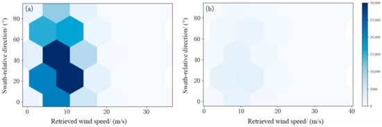
Figure 1.
Principle diagram of MUDH technique, taking a two-dimensional histogram as an example. (a) The histogram used to accumulate the total number of WVCs; (b) the histogram used to accumulate the number of rain-contaminated WVCs.
2.4.2. Construction of Rain Identification Model Based on KNN
In this paper, the K-Nearest Neighborhood (KNN) algorithm was used to build the rain identification model for the HY-2A scatterometer. The algorithm plays an important role in the classification algorithm for the reason that it is simple, effective, and has a mature theoretical basis [26,27]. The idea of this algorithm is that if most of the K samples around a target point in the feature space belong to a certain category, then the sample also belongs to this category, where K samples are instances of the correct classification. As shown in Figure 2, the green dot is a target point to be classified. When k is equal to 3, the algorithm selects the 3 nearest samples, of which 2 belong to Class A and 1 belongs to Class B, so the target point will be classified as Class A. However, when k is equal to 5, the algorithm selects the 5 nearest samples, of which 2 belong to Class A and 3 belong to Class B. As such, the target point will be classified as Class B at this time.
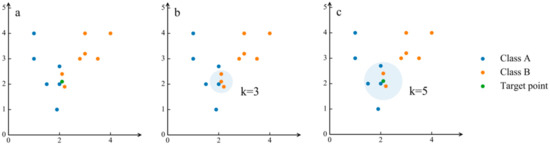
Figure 2.
Principle diagram of KNN algorithm. (a) Target point and samples; (b) the result of k equal to 3; (c) the result of k equal to 5.
However, the KNN algorithm has the problem of low efficiency in the face of high-dimensional data. In order to improve the search efficiency of KNN, the K-Dimension tree was adopted in this study to index the data in the six-dimensional parameter space, and the searching method of greedy backtracking was used to search for k-nearest neighbors around the target point [28,29,30,31,32,33]. The KD tree can be used to avoid searching the most data points, thus reducing the computation of searching, and the average computational complexity of the search with this method is O (logN). The technical route is shown in Figure 3. In the process of constructing the KD tree, although the NBD and ABD of some WVCs cannot be calculated, they can be continued to be used after the missing value is marked as −999. As a result, the rain identification model constructed in this way is applicable to all WVCs. Furthermore, there is no need to build different rain identification models for the outer and inner swath.
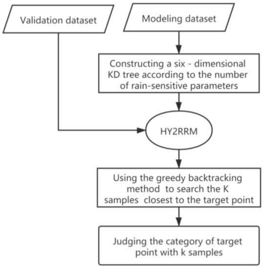
Figure 3.
Technology flow of the KNN algorithm.
3. Results
3.1. Analysis of Rain-Sensitive Parameters
A one-way ANOVA was used to analyze the difference of each parameter between the rain-contaminated data (precipitation > 0.1 mm/h) and rain-free data (precipitation < 0.1 mm/h) to determine the significance of the influence of rain on each parameter. As shown in Figure 4, for the five rain-sensitive parameters, the significant p values between rain-contaminated data and rain-free data were all less than 0.05, indicating that rain had a significant impact on the five rain-sensitive parameters. Then, the response of these five parameters to the change of precipitation was further analyzed by using the method of multiple comparisons.
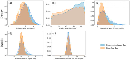
Figure 4.
Comparison of the influence of rain on sensitive parameters. The rain-sensitive parameters are as follows: (a) retrieved wind speed; (b) relative wind direction; (c) normalized beam difference; (d) mean deviation of NRCS; (e) beam difference between fore and aft.
The experiment divides the precipitation into five levels according to the standard of the China Meteorological Administration: no rain, light rain (0.01–0.41 mm/h), moderate rain (0.41–1.25 mm/h), heavy rain (1.25–2.5 mm/h), and rainstorm (>2.5 mm/h). Because the five parameters did not satisfy the F-test, the Tamhanes’ T2 method was used for multiple comparisons [34]. The experimental results are shown in Figure 5. The box plot shows the distribution of data under different precipitation levels. The line segment graph represents the difference in the mean values of the data at adjacent levels. The closer the difference to zero, the smaller the difference between the two groups of data, indicating that the parameter has no significant change within this precipitation range. In addition to the retrieved wind speed and the retrieved wind direction relative to the along-track direction being very sensitive to rain, other parameters only change significantly under moderate precipitation or above. As a consequence, the rain identification model constructed by these parameters may easily misjudge the rain-contaminated data with a precipitation between 0.01 mm/h and 0.41 mm/h as rain-free data.
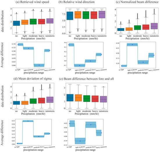
Figure 5.
Response of sensitive parameters to precipitation changes. The rain-sensitive parameters are as follows: (a) retrieved wind speed; (b) relative wind direction; (c) normalized beam difference; (d) mean deviation of NRCS; (e) beam difference between fore and aft.
3.2. Result and Accuracy Verification of the Model
3.2.1. Comparison and Analysis of Experimental Results
In this study, we conducted several tests to evaluate the performance of the rain identification model under different rainfall thresholds. In addition, since KNN can predict the probability of rain for each sample (if the probability is higher than the threshold, the data can be judged as rain-contaminated; otherwise, the data are judged as rain-free), the probability threshold was set to 0.5 and 0.6 to establish HY2RRM0.5 and HY2RRM0.6. Then, the confusion matrix was used to evaluate the performance of each model. The selected evaluation indexes were as follows: (1) accuracy: the proportion of correctly classified data in the total data; (2) rain identification accuracy: the proportion of the data correctly predicted as rain-contaminated data to the actual rain-contaminated data; (3) false alarm percentage: the proportion of data that were predicted to be rain-contaminated but were actually rain-free; (4) missed rain percentage: the proportion of data that were predicted to be rain-free but were actually rain-contaminated; (5) rejection rate: the proportion of rain-contaminated data flagged by the model to the total data. The results are shown in Table 1.

Table 1.
Performance comparison between HY2RRM0.5, HY2RRM0.6, and MUDH_HY2.
By comparing HY2RRM models with different rain thresholds, the variation trend of the performance of HY2RRM models was found to be consistent with our expectations. With the increasing rain threshold, the accuracy, rain identification accuracy, and false alarm percentage of HY2RRM tended to increase, while the missed rain percentage and rejection rate tend to decrease. However, the effect of rain threshold was less than expected, especially for the accuracy and rejection rate. The average change rates of the accuracy and rejection rate of HY2RRM0.5 were only 0.91% and −8.47%, while the average change rates of HY2RRM0.6 were only 1.22% and −9.59%. Compared with the rain identification models with different probability thresholds, HY2RRM0.5 had a higher rain identification accuracy and a lower missed rain percentage, indicating that HY2RRM0.5 was more sensitive to rain and could identify as much rain-contaminated data as possible. The accuracy of HY2RRM0.6 was higher, and the rejection rate was only half that of HY2RRM0.5. The higher the probability threshold, the stricter the criteria for rain identification will be, and the fewer data will be screened out. As a result, HY2RRM0.6 was found to be conducive to maintaining the integrity of data. It can be seen that the setting of the rain threshold and probability threshold is a process used to judge and weigh the accuracy and the rain identification accuracy.
Compared with the comparative experiment, the HY2RRM with a 2 mm/h rain threshold exhibited significant advantages. When the probability threshold was set at 0.5, the accuracy and false alarm percentage of the model were not significantly different, but the rain identification accuracy was 24.36% higher and the missed rain percentage was 1.16% lower. When the probability threshold was set at 0.6, the rain identification accuracy and missed rain percentage of the model were not significantly different, but the accuracy was 14.04% higher and the false alarm percentage was 13.88% lower. Thus, HY2RRM was shown to be able to completely replace MUDH_HY2 in this experiment, indicating that the effect of MUDH being transplanted to HY-2A satellite is not good.
In the case that the amount of rain-contaminated data is far less than the rain-free data, the receiver operating characteristic (ROC) can better show the performance of the HY2RRM with different rain thresholds. The ROC represents the distribution of the rain identification accuracy and the missed rain percentage of HY2RRM under different probability thresholds. When one ROC completely includes another ROC in the lower right corner, it indicates that the classifier has a better effect than the latter. As shown in Figure 6, among all the curves, the curve of the model with the rain threshold set at 4 mm/h was the closest to the coordinate point (0.0, 1.0). It can be considered that this model exhibited the best explanatory power of identifying rain. However, whether it can be used as the final choice still needs to be further tested to observe the inversion accuracy of the filtered rain-contaminated data.
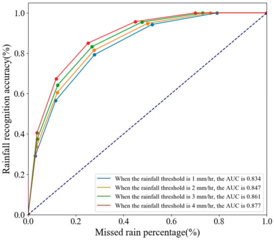
Figure 6.
ROC curve under different rain thresholds.
3.2.2. Comparison of Inversion Accuracy before and after Rain Identification
To observe the effect of the HY2RRM on the quality of the retrieved wind field, the wind measurement accuracies (WindL2B–WindECMWF) of rain-contaminated and rain-free data flagged by HY2RRM and ECMWF were calculated, respectively. Statistical indicators included the mean absolute deviation (MAD) and mean deviation (MD) of wind speed and direction, as well as the accuracy growth compared to the validation dataset. The specific situation is shown in Table 2. The quality of the retrieved wind field filtered by HY2RRM0.5 or HY2RRM0.6 was significantly improved, and the accuracy increase of retrieved wind speed was more than 11%, which was much higher than the actual situation. Under the same rain threshold, the inversion accuracy of wind speed and direction after HY2RRM0.5 and HY2RRM0.6 filtering showed little difference, with difference rates of only about 4.9% and 2.65%, but the data rejection rate showed a great difference, with difference rates if 40.6% and 51.88%, respectively. With the increase of the rain threshold, the accuracy growth of the retrieved wind speed of data flagged as rain-contaminated by HY2RRM0.5 and HY2RRM0.6 decreased significantly, but the accuracy growth of rain-free data did not change significantly, as shown in Figure 7 and Figure 8. As a result, choosing HY2RRM with a high rain threshold can result in a lower rejection rate, but the improvement effect of the retrieved wind field quality after rain identification will not be very different.
Table 2.
Improvement of wind field quality from HY2RRM0.5 and HY2RRM0.6 under different rain thresholds.
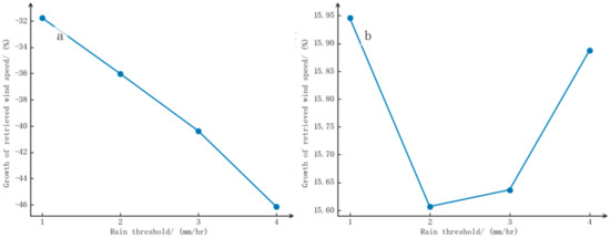
Figure 7.
Influence of HY2RRM0.5 model on accuracy of retrieved wind speed with rain threshold. (a) The result of rain-contaminated data; (b) the result of rain-free data.
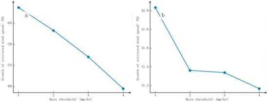
Figure 8.
Influence of HY2RRM0.6 model on accuracy of retrieved wind speed with rain threshold. (a) The result of rain-contaminated data; (b) the result of rain-free data.
In short, the quality of the retrieved wind field was significantly improved after filtering out rain-contaminated data by HY2RRM, but there was no significant difference between HY2RRM0.5 and HY2RRM0.6; the main difference was in the rejection rate. In addition, both the quality improvement effect and the rejection rate exceeded expectations, which indicated that HY2RRM not only flagged most of the data polluted by rainwater, but also many data might have been misjudged due to poor quality.
3.2.3. Validation Case
In this study, an orbit of HY-2A data was selected to verify the accuracy of R4_HY2RRM0.6, the identifier of which is H2A_SM2B20130404_07609. These data were chosen because they contained more rain-contaminated data. In addition, because the geophysical model function of the HY-2A scatterometer has poor inversion accuracy at high wind speed, and the wind speed range of HY2RRM is limited to 3–15 m/s, data with a wind speed greater than 15 m/s were filtered out in the experiment. As shown in Figure 9, the red area is the area where HY-2A data were able to match with ECMWF, the blue point is the rain-contaminated data judged by ECMWF or HY2RRM, and the green point is the rain-free data. The results of this experiment showed that the accuracy was 86.31%, the accuracy of rain identification was 74.33%, the false alarm percentage was 10.52%, and the missed rain percentage was 3.16%, exhibiting no obvious difference from the above statistical results.
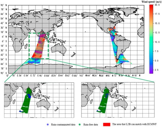
Figure 9.
Situation of rain identification using H2A_SM2B20130404_07609 data. (a) Identification result of ECMWF; (b) identification result of R4_HY2RRM0.6.
4. Discussion
The ideal rain identification model usually has a high classification accuracy, high rain identification accuracy, low data rejection rate, and significant wind field product quality improvement effect. However, in practical applications, these indicators are often difficult to simultaneously obtain, and it is necessary to make a choice. Thus, the criteria of loose and tight rain identification are extended. Loose criteria refer to recognizing as much rain-contaminated data as possible, which is mainly reflected by a low rain threshold and low probability threshold in the study, whereas tightened criteria refer to rigorously identifying rain-contaminated data, which is reflected by a high rain threshold and high probability threshold in the study. The accuracy rate of the loosest HY2RRM in the experiment was 72.95%, the accuracy of rain recognition was 79.27%, the data rejection rate was 33.4%, and the accuracy of the retrieved wind speed and direction increased by 15.94% and 9.7%, respectively. The accuracy of the most tightened HY2RRM was 88.16%, the accuracy of rain identification was 69.61%, the rejection rate for data was 12.1%, and the retrieval accuracy increases for the wind speed and direction were 11.22% and 4.04%, respectively. Thus, it can be seen that, unlike the selection of rain-sensitive parameters, the setting of the probability threshold and rain threshold has no absolute good or bad effect on model performance. It is a process of measuring accuracy and rain identification accuracy, and standards need to be selected according to actual application scenarios. In application scenarios aimed at improving the quality of the retrieved wind field, the integrity of the data needs to be maintained, and incomplete data will seriously affect the usefulness of the model. As a result, it is not acceptable for HY2RRM0.5 to reject about a quarter of the data. In addition, the effect of each HY2RRM on the wind field quality improvement is similar, so the R4_HYRRM0.6 is an ideal choice, but its data rejection rate is still much higher than the actual situation, which needs to be improved in subsequent studies.
MUDH_HY2, in comparison, presents no significant advantages over R2_HY2RRM0.5 and R2_HY2RRM0.6 for the following reasons. On the one hand, the identification effect of MUDH_HY2 is greatly reduced due to the lack of a brightness temperature parameter, which contributes a great deal to the rain identification and is one of the indispensable parameters in rain detection radar. On the other hand, Huddleston did not introduce the processing details in his paper. For example, when using histogram statistics, the distribution of data is diverse, but each bin of the parameter space is not given, so the regularity of some factors is not obvious. In addition, the MUDH essentially calculates the total probability of rain events. Due to the high feature dimensions and the large number of feature grades, data sparsity is inevitably caused. However, no relevant solution was proposed in the technical report, so this study had to use similar methods to deal with this factor, and many details were not handled properly, making the effect of MUDH_HY2 inferior to MUDH. From a technical point of view, it is very difficult to directly transplant the rain identification algorithms of other scatterometers, so the HY-2A scatterometer needs an independently developed rain identification technology.
In contrast, the HY2RRM method built with the KNN algorithm in this study has the following three advantages. First of all, the rain-sensitive parameters used in the construction of the HY2RRM are from the HY-2A scatterometer, which makes the HY-2A scatterometer able to flag rain-contaminated data at any time during measurement without waiting for matching to other external data before processing. Secondly, the KNN algorithm is not sensitive to abnormal data, and the problem of missing parameters in part of the data does not affect the calculation. Moreover, the method does not need to make assumptions on the data and engage in excessive processing to achieve the ideal effect of recognizing rain, and it has strong portability. In contrast, the traditional MUDH rain-flagging technique requires the data attributes to be complete; otherwise, the calculation will be affected. As a result, HY2RRM is applicable to all WVCs, and there is no need to build two rain identification models for inner and outer swath cases as in the method by Huddleston. Finally, different rain thresholds and predictive probability thresholds were used for the test. The false alarm percentage of the HY2RRM was very low, ranging from 0.1% to 4.73%, which indicated that the HY2RRM has a good effect on filtering rain-contaminated data.
5. Conclusions
In this study, observation data based on the HY-2A scatterometer were used for rain identification for the first time. In the experiment, the scattering characteristics of the response of rain to microwaves and the response of the scatterometer to rain were explored, and four conclusions were drawn as follows:
(1) When selecting rain-sensitive parameters, in addition to the conventional parameters, such as the retrieved wind speed, the swath-relative direction, and the normalized beam difference, new parameters can be expanded through many tests, such as the beam difference between fore and aft, the node number of WVC, and the mean deviation of backscattering coefficient. The experiment found that these parameters were significantly affected by rain. The retrieved wind speed and the swath-relative direction are the most sensitive parameters to rain, and the other parameters only have significant changes when the intensity of rain is moderate or above. In addition, because the parameters required for the calculation of these parameters are all from the HY-2A scatterometer itself, there is no need to match external data.
(2) Besides the selection of rain-sensitive parameters, the criteria of rain identification are also the parameters that affect the performance of the rain identification model. In this study, the parameters affecting the criteria were the rain threshold and prediction probability threshold, and the setting of the threshold is a process of weighing the model accuracy and rain identification accuracy. Through many experiments and comparisons, it is considered that R4_HYRRM0.6 is an ideal choice in application scenarios aimed at improving the quality of the inversion wind field. Its accuracy is 88.16%, the accuracy of rain identification is 69.61%, the data rejection rate is 12.1%, and the precision increase of retrieved wind speed and direction is 11.22% and 4.04%, respectively.
(3) The experiment attempted to transplant the traditional MUDH rain-flagging technique to the HY-2A satellite, but due to the hardware facilities and processing technology of the HY-2A scatterometer, the effect of MUDH-HY2 was greatly reduced, which shows that it is not advisable to directly transplant the rain identification technology of other satellites from a technical point of view. The HY-2A satellite needs to have its own rain identification technology.
(4) HY2RRM can overcome some of the limitations of MUDH. The algorithm is insensitive to abnormal data and can achieve an ideal rain identification effect without making assumptions and engaging in excessive data processing. It has strong portability and is suitable for all WVCs.
The HY2RRM provides a possible way to improve the inversion accuracy of the Ku-band scatterometer wind field further, but there are some limitations to the experiment; for example, the data rejection rate is much higher than the actual situation, and because the geophysical model function of the HY-2A scatterometer has poor inversion accuracy at high wind speed, the wind speed range is limited to 3–15 m/s. These problems warrant further research. In addition, the method is dependent on a user-defined threshold. Future studies on the automatic selection of a threshold will be able to improve the applicability of the method to different scenarios and datasets.
Author Contributions
Conceptualization, X.X.; investigation, Y.P. and X.X.; methodology, Y.P., X.X. and M.L.; data curation, Y.P., F.Y. and Y.Z.; visualization, Y.P., L.R. and F.Y.; formal analysis, X.X. and M.L.; validation, L.T. and Y.Z.; writing—original draft, Y.P. and X.X.; writing—review and editing, X.X. and L.R.; funding acquisition, X.X.; supervision, X.X. and M.L.; All authors have read and agreed to the published version of the manuscript.
Funding
This research was funded in part by the National Natural Science Foundation of China (Grant Numbers: 41876204, 41476152), and in part by the Special Fund Project for Marine Economic Development of Guangdong Province (Grant Number: GDNRC [2020]013).
Institutional Review Board Statement
Not applicable.
Informed Consent Statement
Not applicable.
Data Availability Statement
The data presented in this study are available on request from the corresponding author.
Acknowledgments
The authors are very grateful to the National Satellite Ocean Application Service, the National Data Buoy Center, and the European Centre for Medium-Range Weather Forecasts for providing the HY-2A scatterometer data, the buoy data, and the reanalysis wind field data, respectively. The authors are also deeply indebted to all the reviewers of this paper for their instructive suggestions.
Conflicts of Interest
The authors declare no conflict of interest.
References
- Tsai, W.Y. Overview of NASA Scatterometers Projects. In Proceedings of the International Geoscience & Remote Sensing Symposium, Firenze, Italy, 10–14 July 1995; Volume 2, pp. 1564–1566. [Google Scholar]
- Allen, J.R.; Long, D.G. An analysis of SeaWinds-based rain retrieval in severe weather events. IEEE Trans. Geosci. Remote Sens. 2005, 43, 2870–2878. [Google Scholar] [CrossRef]
- Lin, W.; Portabella, M.; Stoffelen, A.; Turiel, A.; Verhoef, A. Rain Identification in ASCAT Winds Using Singularity Analysis. IEEE Trans. Geosci. Remote Sens. 2014, 11, 1519–1523. [Google Scholar] [CrossRef][Green Version]
- Zhou, X.; Yang, X.F.; Li, Z.W. Rain effect on C-band scatterometer wind measurement and its correction. Acta Phys. Sin. 2012, 61, 532–542. [Google Scholar]
- Huddleston, J.N.; Stiles, B.W. A multidimensional histogram rain-flagging technique for SeaWinds on QuikSCAT. In Proceedings of the IEEE International Geoscience & Remote Sensing Symposium, Honolulu, HI, USA, 24–28 July 2000; Volume 3, pp. 1232–1234. [Google Scholar]
- Lungu, T.; Callahan, P.S. QuikSCAT Science Data Product User’s Manual: Overview and geophysucal data products. Pasadena, CA: Jet Propulsion Lab., 2006. D-18053-Rev A, Ver. 3.0. Available online: https://podaac.jpl.nasa.gov/pub/ocean_wind/quikscat/doc/QSUG_v3.pdf (accessed on 15 May 2020).
- Owen, M.P.; Long, D.G. Simultaneous Wind and Rain Estimation for QuikSCAT at Ultra-High Resolution. IEEE Trans. Geosci. Remote Sens. 2011, 49, 1865–1878. [Google Scholar] [CrossRef]
- Portabella, M.; Stoffelen, A. A comparison of KNMI quality control and JPL rain flag for SeaWinds. Can. J. Remote Sens. 2002, 3, 424–430. [Google Scholar] [CrossRef]
- Mears, C. Detecting rain with QuikScat. In Proceedings of the IEEE International Geoscience & Remote Sensing Symposium, Honolulu, HI, USA, 24–28 July 2000; Volume 3, pp. 1235–1237. [Google Scholar]
- Lin, W.; Portabella, M. Toward an Improved Wind Quality Control for RapidScat. IEEE Trans. Geosci. Remote Sens. 2017, 7, 3922–3930. [Google Scholar] [CrossRef]
- Nie, C.; Long, D.G. A C-Band Scatterometer Simultaneous Wind/Rain Retrieval Method. IEEE Trans. Geosci. Remote Sens. 2008, 46, 3618–3631. [Google Scholar] [CrossRef]
- Plagge, A.M.; Vandemark, D.C.; Long, D.G. Validation and Evaluation of QuikSCAT Ultra-High Resolution Wind Retrieval in the Gulf of Maine. In Proceedings of the IEEE International Geoscience & Remote Sensing Symposium, Boston, MA, USA, 7–11 July 2008; pp. IV.204–IV.207. [Google Scholar]
- Draper, D.W.; Long, D.G. Simultaneous wind and rain retrieval using SeaWinds data. Geosci. Remote Sens. IEEE Trans. 2004, 42, 1411–1423. [Google Scholar] [CrossRef]
- Draper, D.W.; Long, D.G. Evaluating the effect of rain on SeaWinds scatterometer measurements. J. Geophys. Res. Oceans 2004, 109, 1–20. [Google Scholar] [CrossRef]
- Nielsen, S.N.; Long, D.G. A Wind and Rain Backscatter Model Derived From AMSR and SeaWinds Data. IEEE Trans. Geosci. Remote Sens. 2009, 47, 1595–1606. [Google Scholar] [CrossRef]
- Owen, M.P.; Long, D.G. Progress toward validation of QuikSCAT ultra-high-resolution rain rates using TRMM PR. In Proceedings of the Geoscience and Remote Sensing Symposium, Boston, MA, USA, 7–11 July 2008; pp. 299–302. [Google Scholar]
- Owen, M.P.; Long, D.G. Towards Bayesian estimator selection for QuikSCAT wind and rain estimation. In Proceedings of the Geoscience and Remote Sensing Symposium, Honolulu, HI, USA, 25–30 July 2010; pp. 1331–1334. [Google Scholar]
- Battan, L.J. Radar Observation of the Atmosphere; International Convention Record; The University of Chicago Press: Chicago, IL, USA, 1973; Volume 7, pp. 325–350. [Google Scholar]
- Ulaby, F.T.; Moore, R.K.; Fung, A.K. Microwave Remote Sensing: Active and Passive. Volume 1—Microwave Remote Sensing Fundamentals and Radiometry; Addison-Wesley: Norwood, NJ, USA, 1981. [Google Scholar]
- Craeye, C.; Sobieski, P.W.; Bliven, L.F. Scattering by artificial wind and rain roughened water surfaces at oblique incidences. Int. J. Remote Sens. 1997, 18, 2241–2246. [Google Scholar] [CrossRef]
- Bliven, L.F.; Branger, H.; Sobieski, P.; Giovanangell, J.P. An analysis of scatterometer returns from a water surface agitated by artificial rain: Evidence that ring-waves are the main feature. Int. J. Remote Sens. 1993, 14, 2315–2329. [Google Scholar] [CrossRef]
- Trenberth, K.E.; Olson, J.G. An Evaluation and Intercomparison of Global Analyses from the National Meteorological Center and the European Centre for Medium Range Weather Forecasts. Bull. Am. Meteorol. Soc. 1988, 69, 1047–1056. [Google Scholar] [CrossRef]
- Xie, X.T.; Huang, Z.; Lin, M.S.; Chen, K.H.; Lan, Y.G.; Yuan, X.Z.; Ye, X.M.; Zou, J.H. A Novel Integrated Algorithm for Wind Vector Retrieval from Conically Scanning Scatterometers. Remote Sens. 2013, 5, 6180–6197. [Google Scholar] [CrossRef]
- Peng, Y.H.; Xie, X.T.; Lin, M.S.; Pan, C.H.; Li, H.T. A Modeling Study of the Impact of the Sea Surface Temperature on the Backscattering Coefficient and Wind Field Retrieval. IEEE Access 2020, 8, 78652–78662. [Google Scholar] [CrossRef]
- Chen, K.H.; Xie, X.T.; Chen, X.X.; Dai, Y.S.; Huang, Z.; Peng, X. A modified circle median filter approach for SeaWinds scatterometer. J. Trop. Oceanogr. 2006, 25, 31–35. [Google Scholar]
- Zhang, M.L.; Zhou, Z.H. ML-KNN: A lazy learning approach to multi-label learning. Pattern Recognit. 2007, 40, 2038–2048. [Google Scholar] [CrossRef]
- Zhang, H.; Berg, A.C.; Maire, M.; Malik, J. SVM-KNN: Discriminative Nearest Neighbor Classification for Visual Category Recognition. In Proceedings of the 2006 IEEE Computer Society Conference on Computer Vision and Pattern Recognition, New York, NY, USA, 17–22 June 2006; pp. 2126–2136. [Google Scholar]
- Thanh, H. Analyzing and Visualizing Chemical Molecular Properties Using K-Dimension Tree Algorithm. Bachelor’s Thesis, Frankfurt University of Applied Sciences, Frankfurt, Germany, 2020. [Google Scholar]
- Mao, J.; Hu, X.L.; Pan, Q.K.; Miao, Z.; Tasgetiren, M.F. An iterated greedy algorithm for the distributed permutation flowshop scheduling problem with preventive maintenance to minimize total flowtime. In Proceedings of the 39th Chinese Control Conference, Shenyang, China, 27–29 July 2020; pp. 1507–1512. [Google Scholar] [CrossRef]
- Nie, T.T.; Wu, W.J.; He, Q.C.; Zhang, X.Y.; Sun, Y.; Zhang, Y.H. A greedy algorithm based on joint assignment of airport gates and taxiways in large hub airports. High Technol. Lett. 2020, 26, 71–77. [Google Scholar]
- Nguyen, T.T. Optimal distribution network configuration using improved backtracking search algorithm. Telecommun. Comput. Electron. Control 2021, 19, 301–309. [Google Scholar]
- Schmidt, D.C.; Druffel, L.E. A Fast Backtracking Algorithm to Test Directed Graphs for Isomorphism Using Distance Matrices. J. ACM 1976, 23, 433–445. [Google Scholar] [CrossRef]
- Robert, T. Depth-first search. SIAM J. Comput. 1972, 1, 146–160. [Google Scholar]
- Tamhane, A.C.; Dunlop, D.D. Statistics and Data Analysis: From Elementary to Intermediate; Prentice-Hall: New York, NY, USA, 2000. [Google Scholar]


Publisher’s Note: MDPI stays neutral with regard to jurisdictional claims in published maps and institutional affiliations. |
© 2021 by the authors. Licensee MDPI, Basel, Switzerland. This article is an open access article distributed under the terms and conditions of the Creative Commons Attribution (CC BY) license (https://creativecommons.org/licenses/by/4.0/).