Article

Performance of Camera-Based Vibration Monitoring Systems in Input-Output Modal Identification Using Shaker Excitation

1
School of Engineering, University of Leicester, University Road, Leicester LE1 7RH, UK
2
Faculty of Civil Engineering, Wrocław University of Science and Technology, Wybrzeże Stanisława Wyspiańskiego 27, 50-370 Wrocław, Poland
3
School of Civil Engineering, University of Leeds, Woodhouse Lane, Leeds LS2 9DY, UK
*
Author to whom correspondence should be addressed.
Remote Sens. 2021, 13(17), 3471; https://doi.org/10.3390/rs13173471
Submission received: 26 June 2021 / Revised: 18 August 2021 / Accepted: 29 August 2021 / Published: 1 September 2021
(This article belongs to the Section Engineering Remote Sensing)

Abstract

:
Despite significant advances in the development of high-resolution digital cameras in the last couple of decades, their potential remains largely unexplored in the context of input-output modal identification. However, these remote sensors could greatly improve the efficacy of experimental dynamic characterisation of civil engineering structures. To this end, this study provides early evidence of the applicability of camera-based vibration monitoring systems in classical experimental modal analysis using an electromechanical shaker. A pseudo-random and sine chirp excitation is applied to a scaled model of a cable-stayed bridge at varying levels of intensity. The performance of vibration monitoring systems, consisting of a consumer-grade digital camera and two image processing algorithms, is analysed relative to that of a system based on accelerometry. A full set of modal parameters is considered in this process, including modal frequency, damping, mass and mode shapes. It is shown that the camera-based vibration monitoring systems can provide high accuracy results, although their effective application requires consideration of a number of issues related to the sensitivity, nature of the excitation force, and signal and image processing. Based on these findings, suggestions for best practice are provided to aid in the implementation of camera-based vibration monitoring systems in experimental modal analysis.

1. Introduction

Camera-based optical motion capture systems (MCS) have been widely used in the vibration monitoring of civil engineering structures in the last few decades due to their non-contact measurement capabilities [1]. The rapid development of camera-based MCS is best reflected in the number of review studies on the subject which contain a wealth of information related to recent advances in technology, methodology, applications, challenges and frontiers [2,3,4,5,6,7,8]. The typical application of camera-based MCS involves the measurement of structural responses to ambient or imposed loading at one spatial location at the time [8,9,10,11,12,13]. A simultaneous measurement of the structural response at spatially-distant points is less common, although single- and multi-camera MCS have been shown to enable this task. Various types of camera systems have been used, including high-speed cameras [14], action cameras (e.g., GoPro) [15], smartphones [16], consumer-grade digital cameras (CGC) [17], high resolution video cameras [18], stereo cameras [19], multi-camera systems [20,21,22], and camera systems on board of unmanned autonomous vehicles (UAV) [23,24]. The obtained data are most often used to extract modal frequencies and mode shapes [15,18,25,26], and very rarely damping [20,21,22], using various operational modal analysis (OMA) algorithms [15,26] which rely on the measurement of the structural response only. The modal parameters established with OMA are used for updating numerical models of structures [25], and for the assessment of load bearing capacity [27], structural serviceability [13,28] and structural health [26,29]. Apart from the structural response measurements, a few studies estimated the dynamic input loads to civil engineering structures using optical MCS [30,31,32]. These loads were generated from humans jumping [30,33] or walking [34], or by passing vehicles [31]. Other studies explored the potential of hybrid instrumentation systems, combining measurements from typologically different sensors, although the main focus of this work has been on recovering more accurate structural response signals [35,36,37,38].
Notwithstanding the applicability of OMA in dynamic characterisation of civil engineering structures [39], its inherent limitation is associated with the unknown force input. This makes it difficult to obtain the modal mass (i.e., a measure of the mass being mobilised for a given mode), and hence scale the mode shapes. Although several propositions have been put forward to overcome this limitation, they rely on various interventions introducing changes in local mass or stiffness of the structure, which can be impractical to apply on large-scale structures, or require a high fidelity numerical model, which is often difficult to obtain [40,41]. Consequently, modal mass is often overlooked in the dynamic characterisation of structures [42]. However, modal mass is an important design parameter as it governs the dynamic behaviour of structures subjected to dynamic actions (e.g., due to wind and humans), as encapsulated by the Scruton number [43] and pedestrian Scruton number [44,45]. Therefore, classical experimental modal analysis (EMA), relying on the measured input force and output response, is favoured in the full dynamic characterisation of structures. Within this context, the only study known to the authors reporting the modal mass based on measurements from camera-based MCS is that of Kalybek et al. 2021 [46]. An instrumented hammer was used to provide excitation force to a simple spatial structure monitored with various optical MCS. The estimates of modal frequencies and mode shapes were found compatible with those obtained with accelerometry and laser Doppler vibrometer (LDV), while the maximum error magnitudes in the modal damping and mass for modes at 2.7, 8.7, 13.5 and 18.7 Hz were all within 12% and 20%, respectively. However, shaker excitation is often preferred over an instrumented hammer in modal testing, as it generally enables a better signal-to-noise ratio [47]. An accurate determination of modal damping and mass is of increasing importance, considering the advances in engineering materials coinciding with trends towards building lighter and slenderer structures, which are becoming increasingly susceptible to dynamic excitation. However, these dynamic system parameters are rarely reported, even in the case of carefully-arranged laboratory studies. The main reason for that is the significant uncertainty in the determination of modal damping and mass associated with the variety of damping mechanisms and modelling simplifications, and sensitivity to the vibration amplitudes and parameter extraction methods, in particular the type and arrangement of instrumentation systems and data processing algorithms [42,48]. This uncertainty reveals itself in the discrepancy between the estimated modal damping and mass relative to the benchmark, e.g., an instrumentation system of higher accuracy and sensitivity, reaching several dozen percent [46,48,49].
Although the interest in camera-based MCS stems from contactless monitoring of full-size structures, laboratory-based tests allow the performance of these systems to be scrutinised while removing error sources associated with the outside environment, e.g., wind and illumination changes, and random unmeasured loads. Apart from simple structural elements, such studies generally include scaled-down and simplified models of buildings [19,23,50], bridges [51], and grandstands [30]. Therefore, this approach is also adopted in this study.
Considering the above points and building on the work presented in [46], the purpose of this study was to assess the performance of optical MCS in experimental modal analysis using shaker excitation. To this end, the behaviour of a scaled model of a cable-stayed bridge set in a laboratory environment was investigated subjected to pseudo-random white noise-type and sine chirp excitation. The response of the bridge was measured with a set of wired accelerometers and two motion tracking algorithms available in an open access domain, relying on videos collected with a consumer-grade digital camera. A complete set of modal parameters was used in benchmarking of the performance of optical MCS against accelerometery, including modal frequency, damping, mass and mode shapes. To the best of the authors’ knowledge, this is one of the first studies exploring the performance of camera-based MCS in the context of EMA conducted with a shaker.
The rest of the paper is organised as follows. The tested structure, instrumentation and data processing is discussed in Section 2. Section 3 presents the main results, starting from the assessment of data quality, through data processing considerations associated with the optical MCS, to a complete set of modal parameters. The results from Section 3 are discussed in Section 4. Concluding remarks are given in Section 5.

2. Materials and Methods
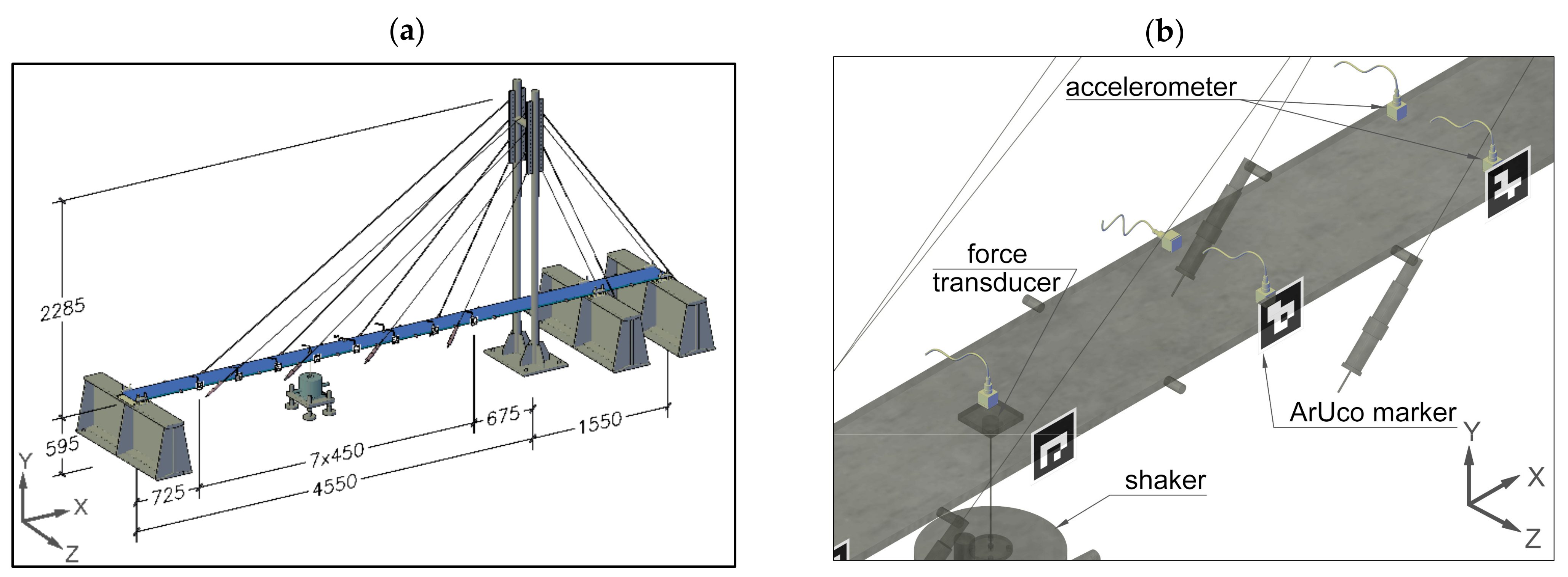
Four forced vibration tests were conducted on a scaled model of a cable-stayed bridge set in a laboratory environment. The whole experimental campaign, including the deployment of the instrumentation systems, lasted three hours and there was no significant variation in the environmental and laboratory conditions during that time. A pseudo-random and a sine chirp excitation with frequency content between 3 and 25 Hz were delivered to the structure with a vibration exciter at two levels of intensity each. The range of excitation frequencies was chosen such as to mobilise the main vertical modes of the deck of the bridge model, as informed by the results presented in [52]. Each test lasted approximately 10 min. A summary of the tests and their identifiers used throughout the paper are presented in Table 1. To enable comparison of the excitation signals’ intensity, Table 1 includes the root-mean-square (RMS) value of the measured excitation force for each test.
An outline of the steps undertaken to capture and process the data used in EMA is presented in Figure 1. The bridge model, instrumentation systems and data processing steps are described in the following sections.

2.1. Bridge Model

The scaled model of a cable-stayed bridge used in this study and the layout of the instrumentation systems are shown in Figure 2. The geometry and dynamic properties of the bridge model were tuned to represent those of real-life full-scale counterparts. The long and short spans of the bridge are 4550 mm and 1550 mm long, respectively, with 50 mm offset from the outer boundaries of the deck to the centre lines of the supports, and the pylon is 2880 mm high. The pylon consists of two legs, each equipped with a cable anchorage plate at the top, connected by a cross-beam. The short span has an auxiliary support enabling longitudinal movement. The deck is made of a solid steel plate 15 mm thick and 250 mm wide. Four pairs of cable stays connect the long span of the bridge to the pylon, back tied on the other side to two anchor blocks by two pairs of cable stays. The deck, sitting 595 mm above the ground, is fixed against longitudinal movement at the pylon but is free to rotate, and free to move longitudinally over all other supports. The bridge model has low frequency modes with relatively low damping. A detailed description of the bridge model can be found in [52].

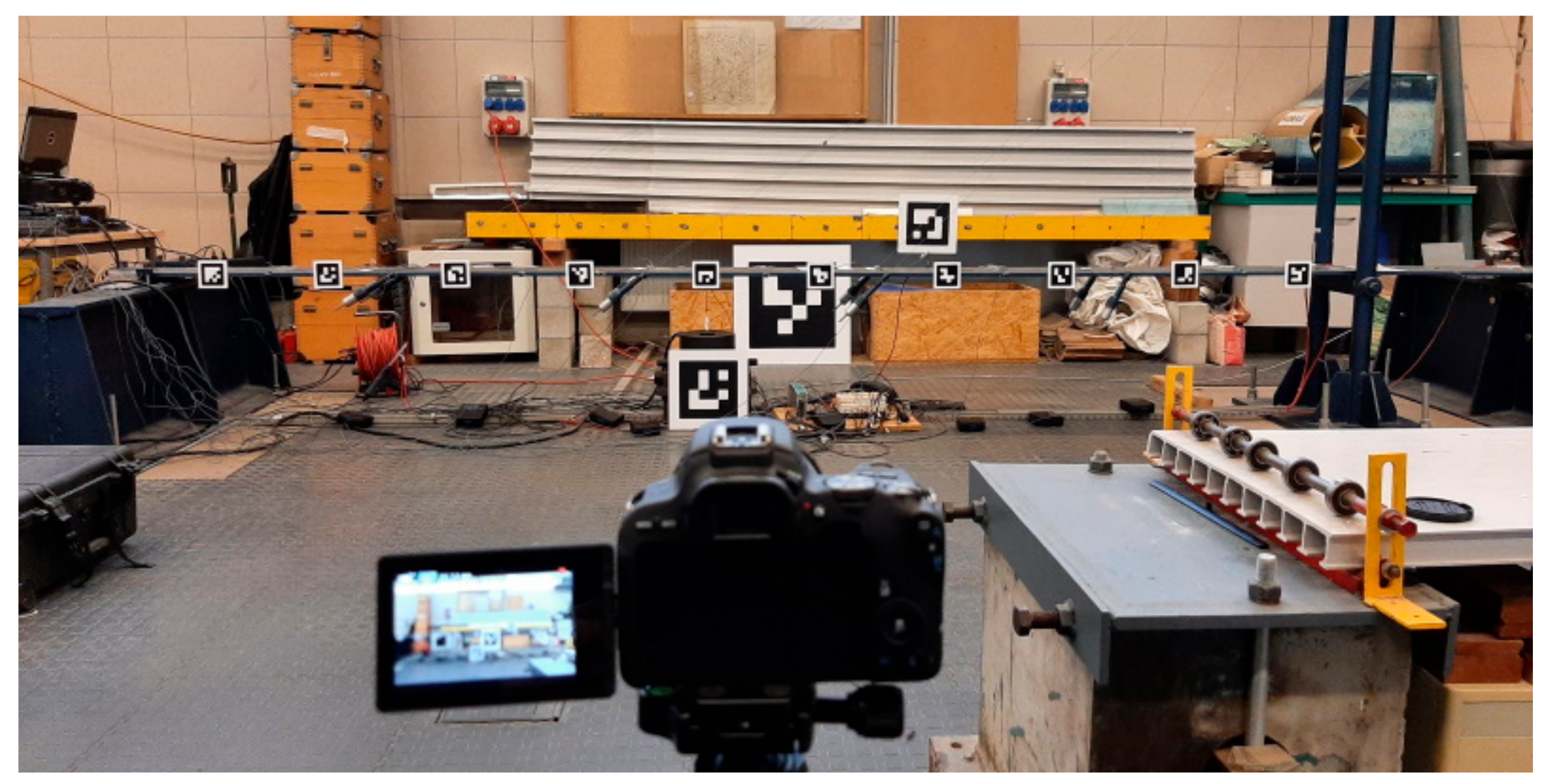
2.2. Instrumentation

The instrumentation systems included wired accelerometers, vibration exciter (electromechanical shaker) and optical motion capture system. Basic specification of the instrumentation systems as provided by the manufacturers is given in Table 2, and a more detailed description is given in Section 2.2.1, Section 2.2.2 and Section 2.2.3. The vibration exciter and accelerometers were connected to Brüel & Kjær PULSE data acquisition system operating with resolution of 24 bit and frequency of 4096 Hz.

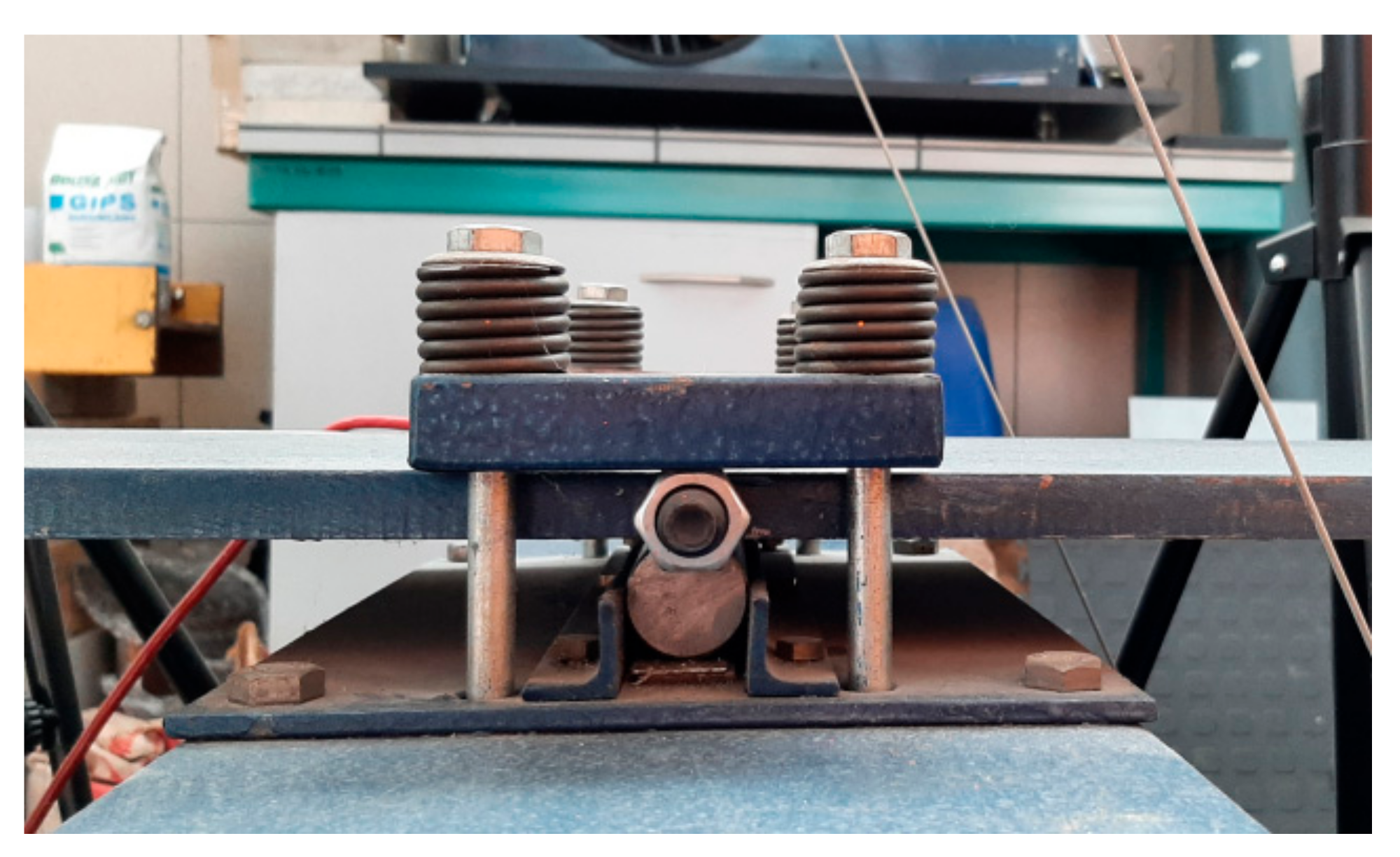
2.2.1. Vibration Exciter

The excitation force was delivered via a Brüel & Kjær Type 4808 permanent magnetic vibration exciter with a force rating of 112 N. Although the range of fully controllable excitation frequencies of the shaker starts at 5 Hz, the shaker is capable of delivering force at lower frequencies, albeit with lesser controllability. The shaker was mounted on a rigid plate supported by the laboratory strong floor and attached to the deck with a stinger via a Brüel & Kjær DeltaTron® 8320-003 force transducer, centrally in the transverse direction and 2.075 m away from the axis of the support furthermost from the pylon. The pseudo-random white noise excitation and sine chirp excitation, with a frequency content up to 25 Hz, were applied to the structure, each at two levels of intensity as defined in Table 1. The rate of the frequency sweep for the sine chirp excitation was 0.037 Hz/s. Having two types of excitation signal served to strengthen confidence in the obtained modal results but also to examine whether the performance of the optical vibration monitoring systems differ in this respect. The pseudo-random and sine chirp excitations were chosen because they prevent bias error and offer a good signal-to-noise ratio [47] (p. 316). An important consideration in the case of pseudo-random excitation is that, although the inherent periodicity of the signal avoids leakage (i.e., spread of energy over frequency bins), the same force is effectively applied to the structure repeatedly over the duration of the test [53] (p. 167). Therefore, the influence of slight nonlinearities and random inputs will not be removed due to averaging to the same extent as in the case of periodic random excitation. Examples of the measured force and response at the point of application of force for T2 and T4 are shown in Figure 3. The repeating patterns of the input force and output acceleration can be seen for pseudo random excitation in Figure 3a,b, respectively. The three parts of the response to sine chirp excitation in Figure 3b for which the amplitude modulus grows beyond 2 m·s−2 correspond to the periods in which the harmonic components of the excitation signal are passing through the natural frequencies. These three parts correspond to the dips in the sine chirp excitation force in Figure 3a which indicate that the deck is moving away from the shaker at resonances [47] (p. 316).

2.2.2. Accelerometers

Acceleration of the deck was measured with ten Brüel & Kjær miniature DeltaTron 4507 B005 accelerometers sitting in dedicated clips attached to the deck with hot melt glue. Seven accelerometers were mounted along the edge of the bridge’s main span facing the camera, as shown in Figure 2a. The locations of these accelerometers correspond to the locations of fiducial markers used with the optical MCS. Therefore, only these seven accelerometers and the corresponding fiducial markers were used to measure the bridge model response for the use in EMA reported in Section 3.2. There were two accelerometers mounted on the other side of the deck, as shown in Figure 2b, to check for horizontal and torsional modes. Another accelerometer was collocated and coaxial with the force transducer mounted on the shaker’s stinger, except that it was mounted on the top rather than bottom side of the deck, to be able to obtain direct point frequency response functions (FRF) hence scale the mode shapes for calculating modal mass.

2.2.3. Optical Motion Capture System

Optical MCS consisted of a Canon EOS 200D with DIGIC 7 processor and a Canon 20 mm lens consumer-grade camera, hereafter referred to as CGC, and a set of fiducial markers based on ArUco library [54], facilitating feature recognition and tracking, as shown in Figure 4. A set of ten 80 × 80 mm ArUco markers with a 10 mm white border was used, such that each marker was 100 × 100 mm in total. The markers were printed on 5 mm thick laminated Styrofoam boards and attached to the side of the deck facing the camera using hot melt glue. There were ten markers spaced every 450 mm between the pylon and the furthermost support away from the pylon. The data from the two outermost markers were not used in the subsequent analysis as there were fewer accelerometers dedicated to the corresponding measurement of the vertical bridge’s response. The short span of the bridge, having auxiliary support at midspan, was not instrumented as it is relatively stiff and it does not participate significantly in the lowest vibration modes which were of interest. The camera-to-structure distance was 5 m. To maximise the accuracy of measurement, the CGC was positioned at the level of the deck such that the angle of incidence was approximately zero degrees in the middle of the long span of the bridge. The horizontal tilt from the zero degrees incident angle at the middle of the long span of the bridge, established from the recorded videos, was approximately three degrees. These angles are within the range recommended for obtaining reliable camera calibration enabling data to be resolved to real-world (i.e., physical) coordinates. The videos were captured at 59.94 frames per second (fps), with autofocus mode disabled. The arrangement of the optical MCS is shown in Figure 4. The big ArUco markers in the background were used for calibration, i.e., scaling the readings from the camera to world coordinate system.
Two motion tracking algorithms commonly used for structural vibration monitoring and available in an open access domain were used in video post processing—an area-based template matching, hereafter referred to as template matching and denoted as TM, and sparse optic flow, denoted as OF. Both algorithms were implemented in a custom software package written in C++ enabling camera calibration (i.e., compensation for the lens’ distortion), definition of the homography matrix [55] (i.e., specification of the transfer function between the world coordinate system and the image coordinate system), and the assignment of the region of interest (ROI) (i.e., an area within the captured image within which to perform the tracking).
The area-based TM is a method that searches for an area in a frame that best matches the template image. Although the laboratory in which the experiments took place had small windows enabling ambient light to get through, the light intensity fluctuations were rather small during the 2 h testing period. Nevertheless, the normalized correlation coefficient was used as a correlation criterion as it is proven to be the most robust against light intensity fluctuations [56]. Once the areas matching the template image are found within a given video frame, the pixel coordinates are further refined using an enhanced cross-correlation (ECC) interpolation method [57].
The sparse OF estimation is an image processing method that computes the motion or flows of sparse feature points (e.g., edges and corners) between two subsequent images caused by the relative movement between the object and camera. The method first extracts the feature points within the predetermined target ROI using the Shi-Tomasi method [58] and then calculates the optical flow at these points using the Lukas and Kanade OF estimation algorithm [59]. The average coordinates of tracked points for each target area are then estimated.

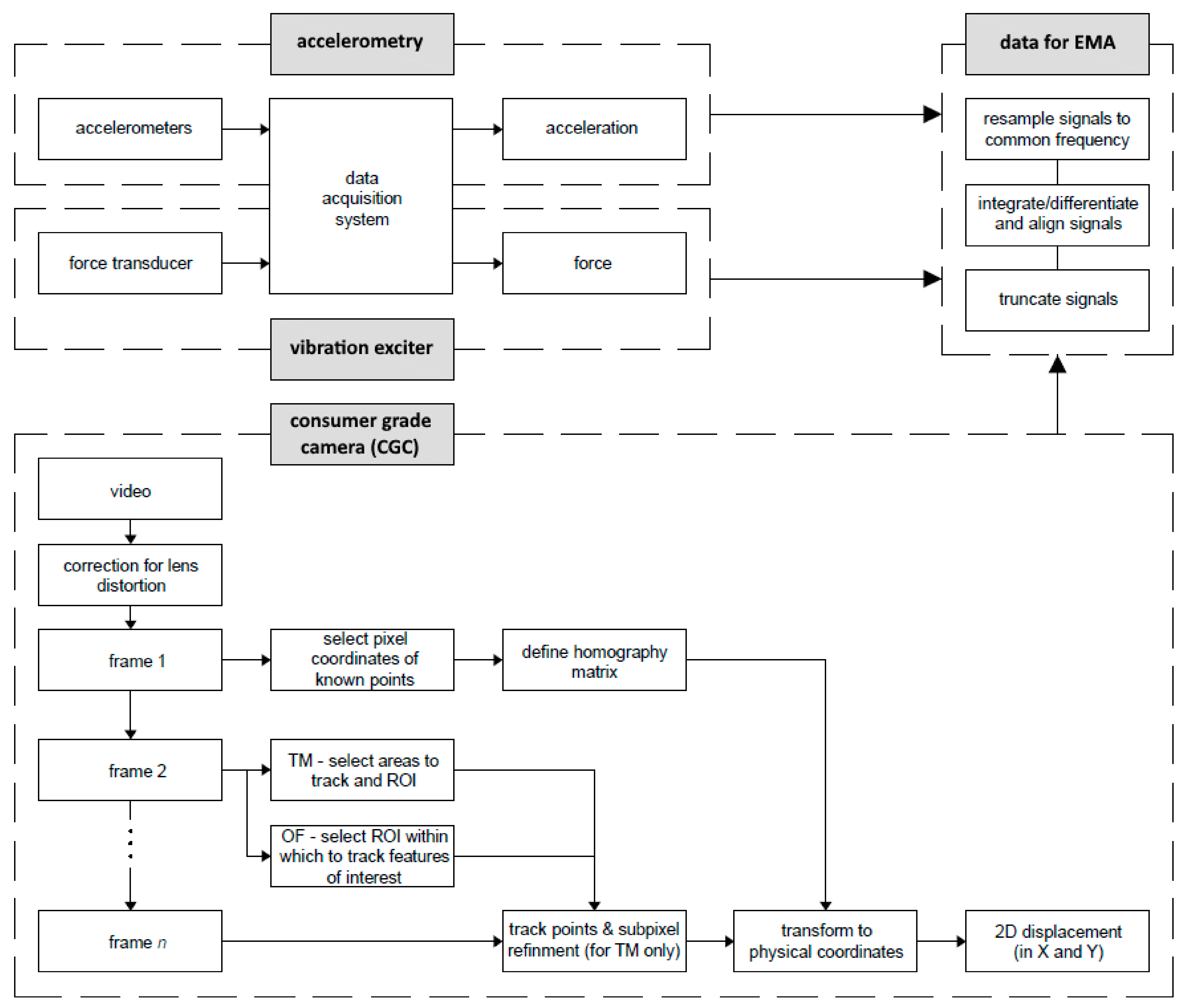
2.3. Data Processing

The data processing consisted of two main steps, signal resampling and time alignment outlined in Section 2.3.1, and modal analysis outlined in Section 2.3.2.

2.3.1. Signal Resampling and Time Alignment

The following procedure was implemented in order to obtain frequency response functions (FRF) for modal analysis. In the first step, the signals from the CGC, accelerometers and force sensor had to be reconciled to a common sampling frequency, which was chosen as 333 Hz. This was dictated by a desire to convert the decimal frequency of the CGC at 59.94 Hz to an integer, while ensuring the sampling frequency is high enough to enable good time alignment between signals from different sensors. To prevent the loss of signal energy associated with this process, the resample function in Matlab R2020b [60] was used, employing a finite impulse response filter. The outcome of this process is shown in Figure 5. It can be seen that the original signals are represented well by the resampled signals, both in the time and frequency domains, insomuch as the difference between them is hardly visible on the plots. Further evidence supporting this point, in particular in relation to the phase relationships, is given in Section 3.1.
Having obtained signals sampled at a common frequency, time-alignment was achieved by matching spatially correspondent acceleration and displacement signals by finding the best fit in the least-squares sense. The point of application of force was chosen for that purpose; to guarantee sufficient motion amplitude. To avoid excessive inaccuracies associated with numerical operations, acceleration and displacement signals were, respectively, integrated and differentiated only once to obtain velocity signals. A 4th order two-way Butterworth band-pass filter with cut-off frequencies at 3 and 20 Hz was applied throughout this process. The results of signal alignment are shown in Figure 6. It can be seen that the match is generally good, although there are small amplitude differences at the peaks.
The time-aligned signals served in modal analysis, outlined in Section 2.3.2.

2.3.2. Modal Analysis

Modal analysis was conducted using Siemens Test.Lab 18.2 PolyMAX™ based on poly-reference least-squares complex frequency domain algorithm.
The input-output relationship in a linear time-invariant system can be quantified in terms of frequency response functions (FRF). The two main methods of estimating FRF are denoted as H1 and H2. They differ in their definition and main assumption. H1 is defined as a ratio of the cross-spectral density of the output with input to the auto-spectral density of the input, and it assumes that the noise at the input is negligible. H2 is defined as a ratio of auto-spectral density of the output to the cross-spectral density of the input with output, and it assumes that the noise at the input is non-negligible. In theory, for noise-free input and output, H1 and H2 should yield the same results, however, this is not the case in real engineering systems. The phase of H1 and H2 is then the same, but the magnitudes differ [61]. H1 and H2 were used in modal analysis, however, since H1 turned out to outperform H2, the reported results are based on H1. H2 is sometimes preferred in the case of shaker excitation to define resonances, as in these conditions the response of the structure is significant but the input signal is relatively weak, hence errors are expected at the input. The choice of the FRF estimator is discussed further in Section 3.1, when considering the FRF obtained with sine chirp excitation which, in theory, should not necessitate windowing of the signals.
To minimise leakage in spectral analysis, windowing and weighting functions are often applied onto the analysed signals to enforce periodicity [53]. The pseudo-random signal contained a number of repeating windows within which the harmonic components were perfectly periodic, see Figure 3. Therefore, the excitation and response signals were truncated such as to cover an integer number of windows while removing transients due to initial conditions and the ramp function. In the case of sine chirp excitation, since the periodicity requirement is in this case was met by default, no weighting functions were initially applied in modal analysis. However, as will be later shown, this turned out to be inadequate for EMA, in particular in the case of optical vibration monitoring systems, and hence this step of signal processing was later introduced.

3. Results

The quality of the recorded data was assessed first and this is reported in Section 3.1, followed by the evaluation of the performance of camera-based MCS in Section 3.2.

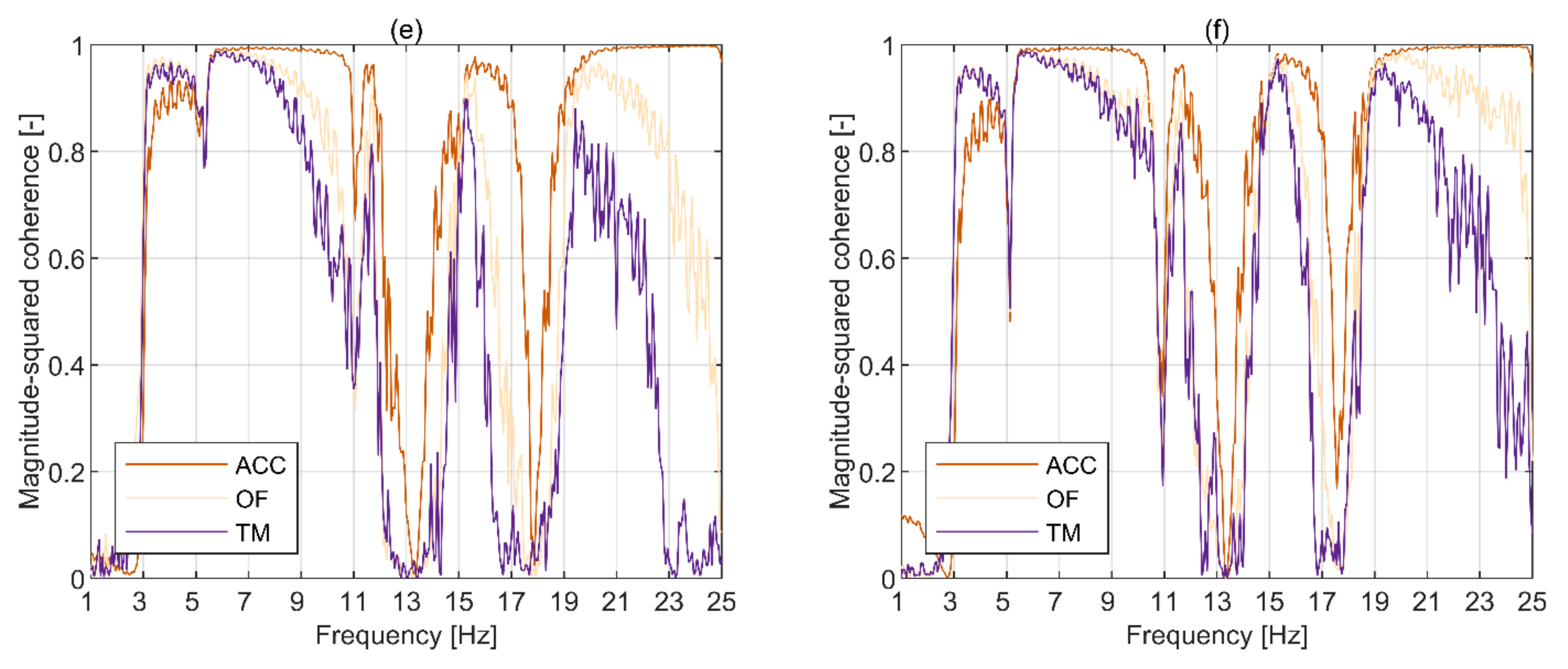
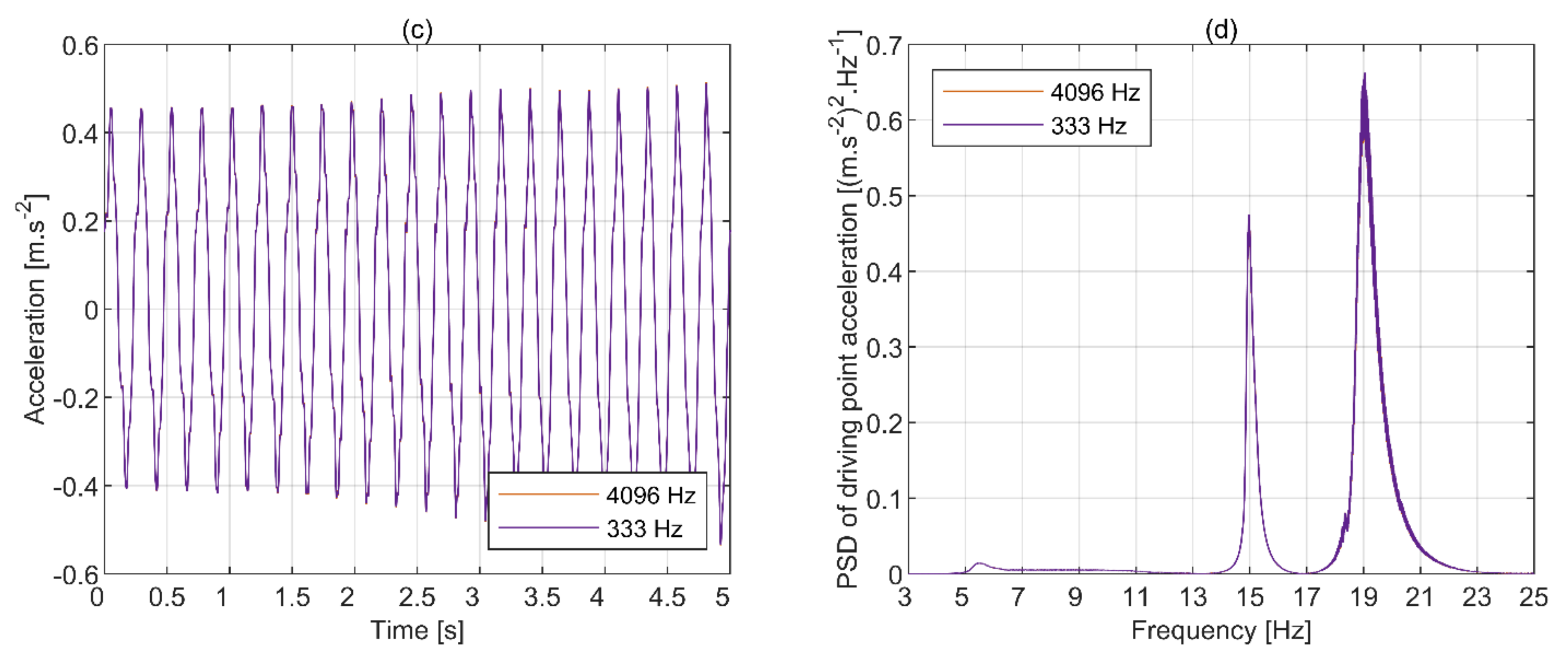
3.1. Quality of Data

An initial assessment of the data quality was made based on the driving point FRF obtained from signals collected with spatially collocated and axially aligned force and response sensors, as shown in Figure 2b. A H1 estimator was used herein under the assumption of the measured input signal being free from noise.
To verify whether the attachment of the shaker to the deck is adequate, the imaginary part of driving point FRF should contain well defined peaks in one direction only. This is shown based on the resampled signals collected during T2 and T4 in Figure 7. There are well defined positive peaks at the frequencies close to those previously identified as the natural frequencies based on a numerical model and experimental data [52], which satisfies this quality requirement. The slight bumps at the frequencies close to 11Hz are also indicative of a natural frequency, however, the instrumentation system was not tuned to capture it, as discussed in the subsequent paragraphs.
In the case of driving point measurement, the FRF magnitude was expected to contain an antiresonance dip between each pair of resonance peaks, while the FRF phase was expected to exhibit a sharp transition from π to 0 rad around the resonances and from 0 to π rad around the antiresonances. For good quality results, the magnitude-squared coherence should take the values close to unity at and around the natural frequencies. To verify this condition, the random error in FRF magnitude at the peaks (which will be later shown to correspond to natural frequencies) was calculated using the formula stated in Brandt [47] (p. 294), after Bendat and Piersol [62]. Furthermore, in theory, no averaging nor windowing should be necessary to obtain smoothly varying FRF magnitudes in the case of sine chirp excitation. All of these issues will be dealt with in turn, for the pairs of tests conducted with the same type of excitation signal.
Figure 8a,b present the FRF mobility magnitude for T1 and T2, respectively, obtained using 71 blocks of 16 s length with a uniform window and 50% overlap, giving a frequency resolution of Δf = 0.0625 Hz. It can be seen that, although the magnitude varies non-smoothly for all signals, it is generally well recovered by the optical systems relative to accelerometry, except at the antiresonances where it fluctuates. Using more averages produces much smoother results, but it masks the fact that the variance of the FRF magnitude for optical MCS is compatible with accelerometry down to the level of the discrete frequency value at and around the two well-defined peaks at the lowest frequencies. The measurements from sine chirp tests were processed in the same way in order to compare the distinct features of FRF between the two excitation methods. For frequencies below approximately 0.5 Hz, not presented explicitly, the FRF magnitude is more reliable for optical systems, since the amplitude and phase error in piezoelectric accelerometers is relatively high at low frequencies.
Out of the four peaks visible in the FRF magnitudes for T1 and T2 in Figure 8a,b, respectively, only three correspond to well defined modes. The split peak at around 11.6 Hz is not well defined with any of the MCS, including accelerometry, which is corroborated by the lack of phase transition in Figure 8c,d, which is clearly visible for the other peaks. According to the numerical model of the bridge created for the purpose of the previous study [52], this peak corresponds to a mode dominated by the vertical bending behaviour of the deck accompanied by the less pronounced bending behaviour of the pylon. However, the setup of the instrumentation systems disallowed its full characterisation, as the shaker was exciting the bridge in very close proximity to a node for that mode, nor was the full modal characterisation the purpose of the current study. Therefore, in the remainder of this study the focus will be on modes with frequencies at approximately 5.2, 15.1 and 19.2 Hz, referred to as mode 1, mode 3 and mode 4, respectively.
The magnitude squared coherence presented in Figure 8e,f for T1 and T2, respectively, is always above 0.81 at the three clearly identifiable peaks in Figure 8a,b, and can reach up to 0.96. The match between accelerometry and optical MCS is generally very good, with the maximum discrepancy of 0.05 for the three peaks. OF typically outperforms TM.
In the case of T1 and T2, the random error at the FRF magnitudes’ peaks (corresponding to natural frequencies) always falls below 3.65% and is almost identical between all MCS for a given test and peak, with differences in the range of 0.006% to 0.079% from the (percentage) error obtained from accelerometry.
Figure 9a,b present driving point FRF magnitudes for T3 and T4 (both involving sine chirp excitation), respectively, obtained without windowing and averaging, having a frequency resolution of Δf = 0.0017 Hz. As could be expected, the magnitude obtained from accelerometry is varying smoothly, except for the frequencies below 3 Hz, for which there was no excitation force, and frequencies between 3 Hz and 4.5 Hz, for which the excitation force controllability and the accelerometer’s performance was not optimal, and for the frequencies above 18 Hz and close to the expected antiresonance dips. However, the FRF magnitudes for the optical MCS show a high level of noise across the whole frequency range shown, except for the resonance peaks. This is due to the low response amplitudes of the bridge at frequencies away from the resonances relative to the sensitivity of the optical MCS and internal data processing algorithms used in the motion extraction. This shows that, despite the harmonic nature of the excitation signal in T3 and T4, the signals need to be windowed and averaged to minimise the errors associated with the internal data processing inherent to optical MCS. Furthermore, the H1 estimator is preferred in this case, since the internal processing of MCS data seems to generate significant noise away from the resonances. The results obtained using 71 blocks of 16 s duration with a uniform window and 50% overlap, giving a frequency resolution of Δf = 0.0625 Hz, are shown in Figure 10.
It can be seen in Figure 10a,b that the FRF mobility magnitude for T3 and T4, respectively, is generally well recovered by the optical systems relative to accelerometry at and around the first peak. For the rest of the peaks, the optical MCS match and underestimate the magnitude obtained from accelerometry at frequencies lower and higher than those at the peaks, respectively. OF generally outperforms TM, and the results are better for T4. In comparison to the results presented in Figure 8 for T1 and T2, which were obtained with the same signal processing method, the match in the FRF magnitude is overall worse, although the magnitude evolves more smoothly, in particular for accelerometry and OF.
There are resonant FRF phase transitions in Figure 10c,d for T3 and T4, respectively, around the frequencies corresponding to the three clearly visible peaks in Figure 10a,b, although the results from TM are relatively noisy, in particular for T3.
The magnitude squared coherence presented in Figure 10e,f for T3 and T4, respectively, is always above 0.7 for accelerometry and OF at the three clearly identifiable peaks in Figure 10a,b, and can reach up to 0.95. The match between accelerometry and OF is very good, with the maximum discrepancy of 0.05 for the three peaks. The magnitude squared coherence for TM takes values as low as 0.62 for mode 4, and the match with accelerometry is much worse, with maximum discrepancy of 0.33.
In the case of T3 and T4, the random error in FRF magnitude at the peaks (which will be later shown to correspond to natural frequencies) always falls below 5.59% and is almost identical between all MCS for a given test and peak, with differences in the range of 0.007% to 0.052% from the (percentage) error obtained from accelerometry.

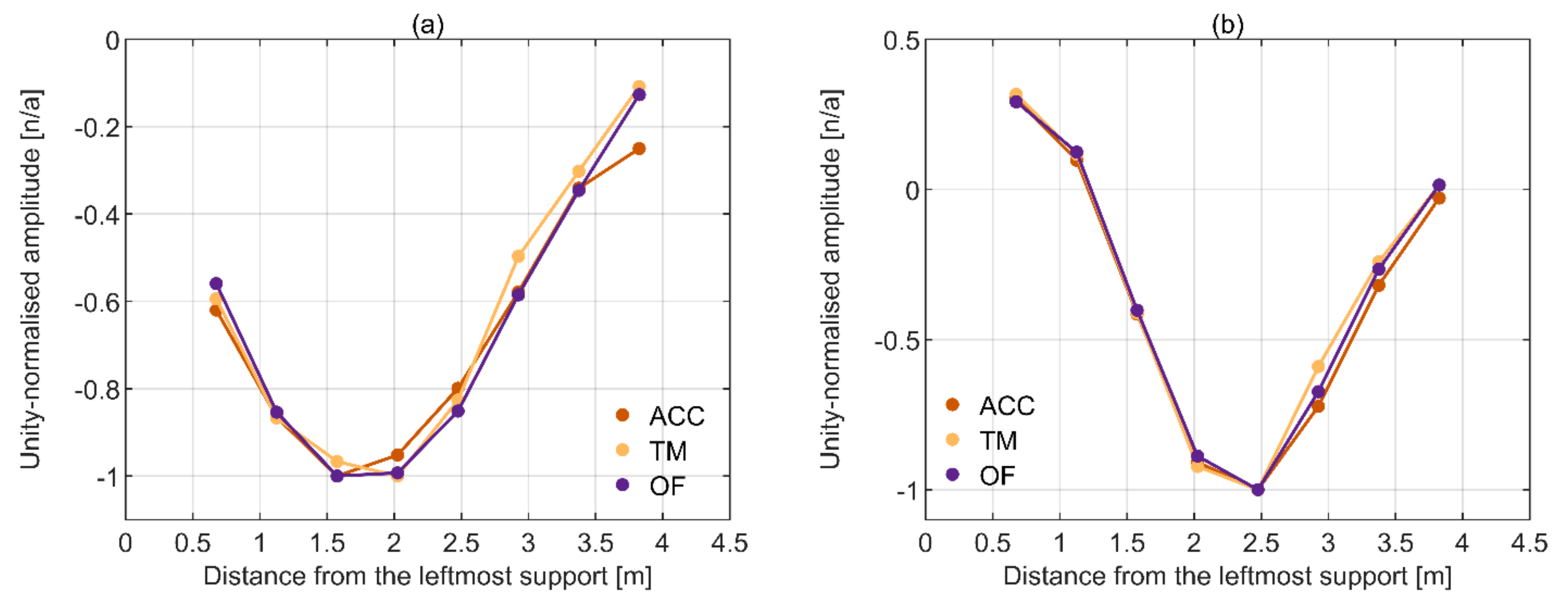
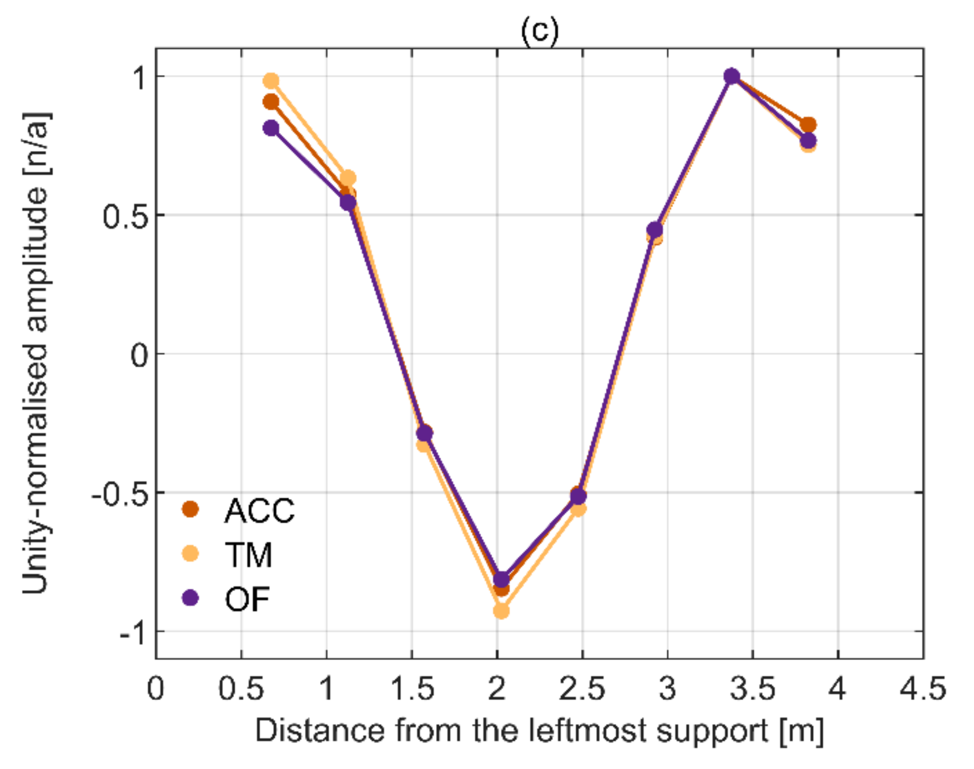
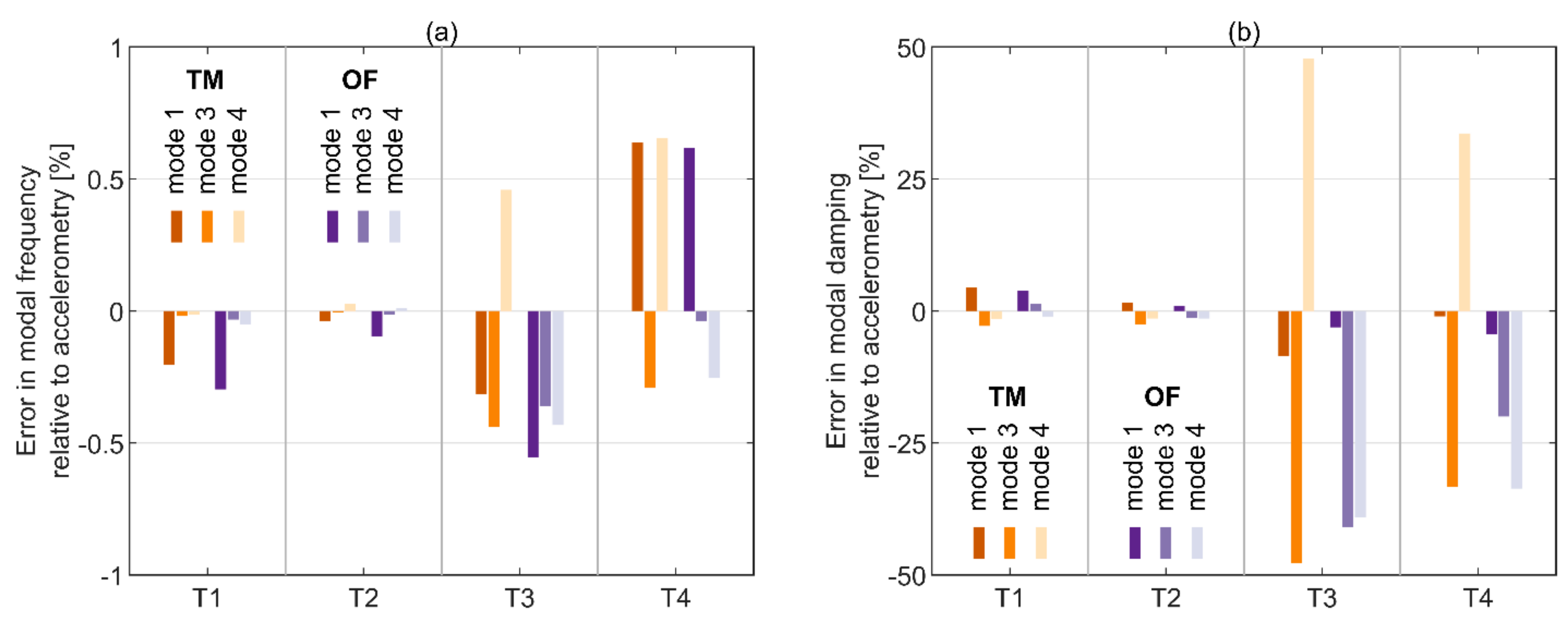
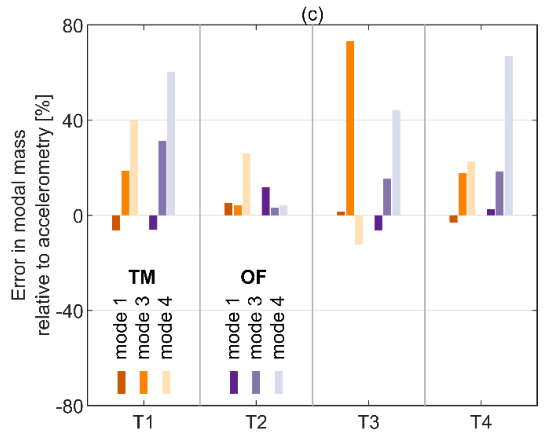
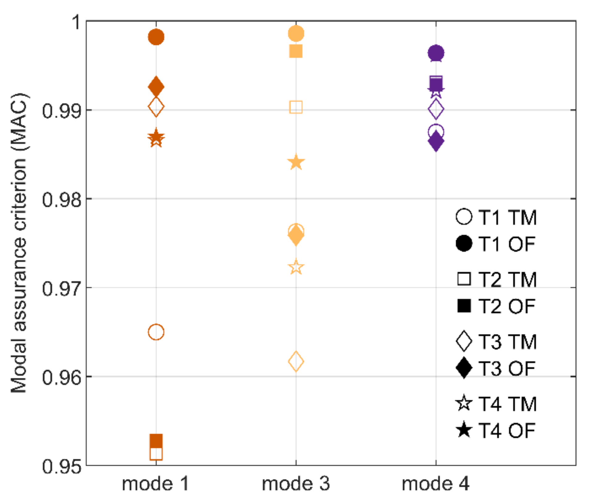
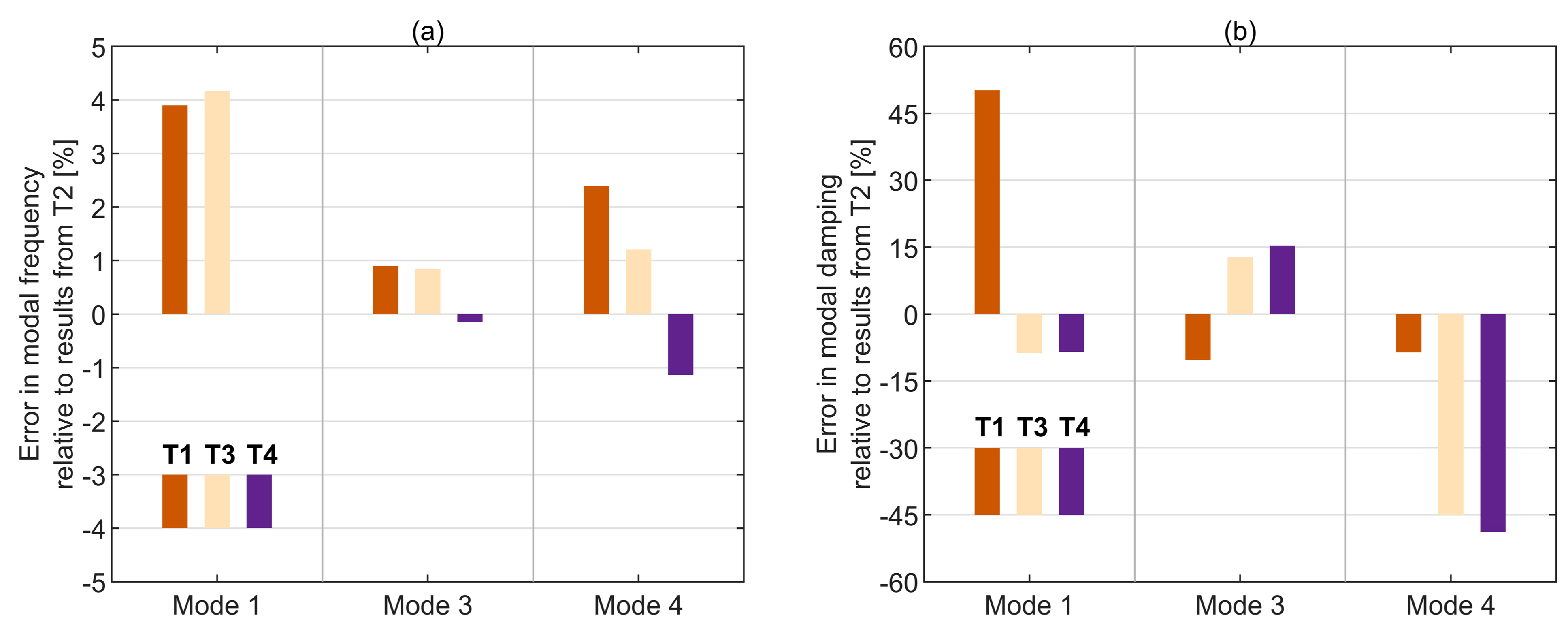
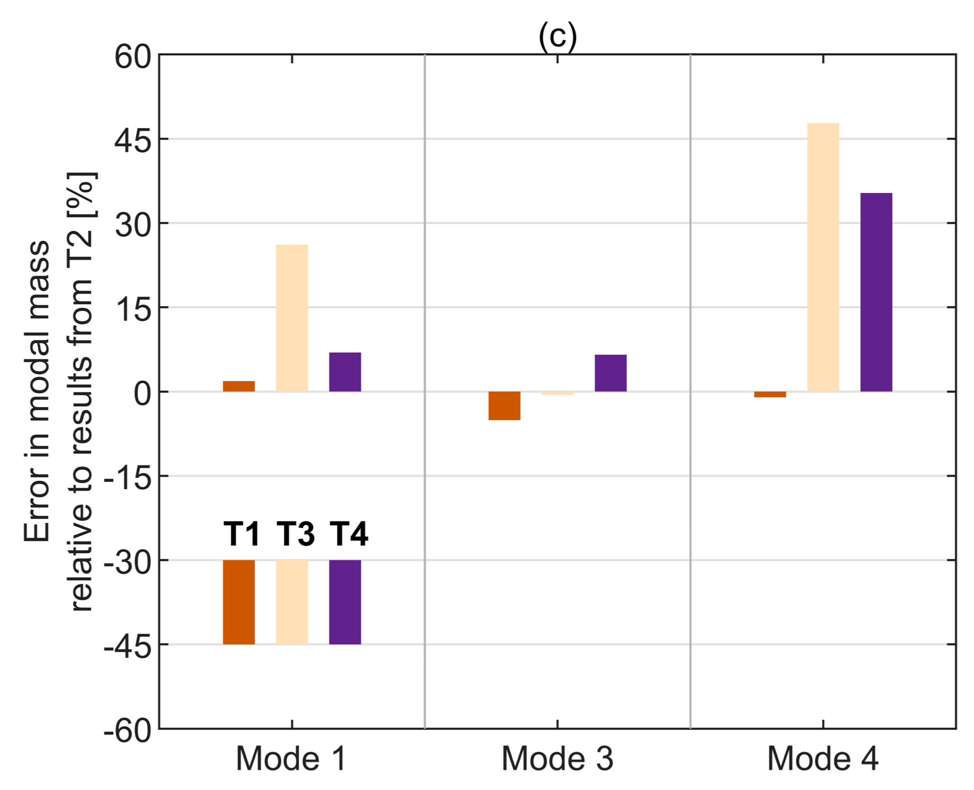
3.2. Modal Parameters

In general, modal parameters are sensitive with regards to the data processing method. In particular, the number of averages and the size of blocks of data chosen in the calculation of the FRF will affect the random and bias errors, respectively. Since these two parameters are co-dependent (i.e., longer block size will produce fewer averages for a given signal length and vice versa), a compromise needs to be found. Furthermore, the block size will affect the frequency resolution of FRF, and hence the accuracy of modal frequency estimates. Therefore, to establish and verify the data processing method, stabilisation diagrams of modal parameters were generated for each of the considered modes. Exemplar outcomes of this process are shown in Figure 11 for T2. The number of independent blocks (or averages), nb, was {1,3,6,9,18,36,72,144}, there was no windowing applied and no overlap. A relatively high variability of modal parameters can be seen for nb < 18. The difference in modal parameters obtained with the three MCS becomes fairly consistent at each nb > 18. To account for these features, a trade-off between the random and bias error, and FRF frequency resolution was established at nb = 36. For consistency and compatibility, this condition was applied in all analyses presented hereafter.
The modal parameters for all tests were established using 36 nonoverlapping blocks of 16 and 16.65 s duration for T1 and T2, and T3 and T4, respectively, applying a uniform window with 50% overlap, giving a total of 71 blocks. The results are shown in Table 3. The percentage errors relative to the results from accelerometry are given in the brackets and, for better observability of trends, visualised in Figure 12.
It can be seen that the modal parameters are sensitive to the excitation method, both in terms of the nature of the excitation signal and its intensity. This is true regardless of the MCS being considered. The modal mass for mode 3 is much higher than for mode 1 and 4, due to that mode significantly mobilising the pylon. The pseudo random excitation consistently yields better results in terms of modal frequency and damping, but similar results in terms of modal (generalised) mass. The closest match between the modal damping and mass is typically found for mode 1. The error magnitude is typically the highest for modal mass, reaching maximum slightly above 73%, and the lowest for modal frequency, reaching maximum at just below 0.66%. Overall, the best set of data in terms of the congruence between the accelerometry and optical MCS comes from tests conducted at a higher excitation intensity (i.e., T2 and T4), and the pseudo-random excitation yields better results than the sine chirp excitation.
The (partial) mode shapes of the longest span of the bridge are shown in Figure 13. The limits on the horizontal axes were scaled to represent the total length of that span between the supports. The 50 mm difference between the span length in Figure 2 and Figure 13 is caused by the offset of the deck’s support furthermost away from the pylon from the boundary of the bridge. It can be seen that the match between accelerometry and optical MCS is generally good.
The modal assurance criterion (MAC) obtained between the mode shapes from accelerometry and optical MCS is presented in Table 4 and, for better observability of trends, visualized in Figure 14.
In all cases the MAC takes values above 0.95, indicating that the eigenvectors derived from accelerometry and optical MCS are well correlated [61] (p. 426). The results obtained with the two image processing algorithms are similar, but OF gives slightly better match with accelerometry on average.

4. Discussion

Three well-defined modes were identified by all instrumentation systems, although the presence of another mode was also evident in the measured signals, but it was not identified explicitly due to the excitation force applied at the node for that mode. This agrees with the predictions of a numerical model of the bridge [52], indicating four modes within the frequency range of interest of this study. All of these modes can be characterised by the bending behaviour of the deck in the plain containing its weak axis, accompanied by the bending behaviour of the pylon in the plane containing the longitudinal axes of the two legs. Although the behaviour of the pylon was not measured explicitly, according to a numerical model of the bridge all the mentioned modes are dominated by the movement of the deck, except for mode 3 which is dominated by the movement of the pylon. This explains the modal mass for mode 3 being significantly greater than for the other modes identified herein.
The modal parameters established during this study differ slightly from those previously reported [52]. There are two main reasons for this. On the one hand, the tension in the cable stays have been changed since the previous tests. On the other hand, the excitation force came from the shaker rather than ambient sources. However, as could be expected, the unity-normalised mode shapes are still in relatively good agreement.
The dynamic behaviour of the bridge was found to be sensitive to the excitation intensity. This applies to the values of the derived modal parameters, but also to the accuracy of results from optical MCS against accelerometry. The best set of data in the latter sense comes from T2 (i.e., test with pseudo-random excitation of higher intensity), where the excitation force had the highest power density of all tests, as shown in Figure 15. In comparison, during T4 (i.e., test with sine chirp excitation of higher intensity), the force power density has only reached half of that in T2. However, the excitation intensity alone does not explain the better match of modal parameters derived from optical MCS for T1 (i.e., pseudo-random test with lower intensity), relative to T4 (and T3, i.e., test with sine chirp excitation of lower intensity). Since the ambient conditions have not changed during the tests, which were conducted in a highly controlled laboratory environment, it seems that the internal processing of data during motion extraction favours the pseudo-random excitation. This is corroborated by the results in Figure 8 and Figure 10, showing a better match of driving point FRF derived from T1 and T2 relative to T3 and T4.
The difference in modal parameters derived from tests at various excitation intensity can be mainly attributed to the behaviour of the bearings away from the pylon, of which an example is shown in Figure 16. At a relatively low level of excitation, (e.g., during T1 and T3), the bearings have significant friction providing restraint against movement, and hence relatively higher identified natural frequencies. The friction at the bearings is overcome by the excitation force during T2 and T4, most likely due to static-kinetic friction transition. Similar behaviour can be observed in real full-scale bridges. For example, for the simply-supported bridge reported in [63], the bearings work in different regimes depending on the vibration amplitude. At relatively small vibration levels, the idealised bearings behave as a pin-pin arrangement, providing restraint against longitudinal movement, and hence higher modal frequencies. However, at higher vibration levels, the idealised bearings behave as a pin-roller arrangement, providing allowance for longitudinal movement, and hence lower modal frequencies. This amplitude dependence hypothesis can be further supported illustratively in view of Figure 17a depicting the comparison of modal frequencies derived solely through accelerometry for all tests relative to the results from T2. Namely, for the pairs of tests with the same excitation type, frequency increases with decreasing response amplitudes (or excitation intensity) for all modes. Furthermore, comparing Figure 17a and Figure 12a, it can be seen that the modal frequency deviation between results from accelerometry and optical MCS, for any mode identified from a given test, typically falls below the modal frequency deviation obtained from accelerometry between tests for that mode. This implies that the potential error from the optical MCS is within the identification uncertainty bounds imposed by the excitation type and intensity in the case of accelerometry.
In general, the errors in modal frequencies are negligible for all modes and all modal results closely follow the qualitative and quantitative outcomes obtained in [46]. An impulse excitation delivered with an instrumented hammer was used therein to mobilise a simpler and lighter structure of which response was measured with a great variety of instrumentation systems. Only the TM outputs are directly comparable to this study. A common feature, beyond the relative magnitudes of deviations established, is that there is no clear trend in the identification errors of modal frequency or damping or mass. This is to say that, relative to the baseline results from accelerometry, a higher mode does not necessarily produce worse modal estimates than a lower and possibly more excited mode when identified through optical means.
Considering all tests and tracking algorithms, the best match between optical MCS and accelerometry was found for mode 1. The error magnitudes in modal frequency, damping and mass fall in this case below 0.65%, 9% and 12%, respectively. As could be expected [46], the most challenging parameter to capture in experimental studies is the modal mass. The deviation from the baseline values from accelerometry reaches in this case up to 74% for mode 3 and TM during T3—the test yielding the worst results overall. Damping, which is also amenable to numerous influences and artefacts, and for this reason has been rarely reported in previous studies probing the performance of optical MCS [64], follows close with deviations reaching up to almost 48% for mode 3 and mode 4, again for TM and during T3. It is worth noting that mode 4 is generally less excited than mode 3 for any test, see e.g., Figure 3b, which is particularly influential on the results obtained from optical MCS measuring the displacement. What seems to be working very well for identifying both modal damping and mass with optical MCS, regardless of the considered mode, is the application of OF during T2—pseudo-random excitation at a sufficient intensity.
To further reveal the limitations of the results obtained with optical MCS, it is also worthwhile considering the deviations between the modal damping and mass obtained during different tests from accelerometry only. These are shown in Figure 17b,c relative to the corresponding results from T2—the test yielding the best results overall.
The error in modal mass seems to be identified with similar and not higher uncertainty than modal damping. However, looking at the results in Figure 12, the opposite is true for the results obtained with optical MCS relative to accelerometry. This is interesting in itself and requires further investigation.
The errors in modal parameters are comparable with those established from testing a structure moved between twelve European laboratories during a project aiming at establishing the consistency in obtaining modal parameters [49]. The variability in the modal frequency, damping and scaling coefficient for mass-normalised modes (rather than modal mass, as presented here) based on measurements from accelerometers was within 4%, 30% and 10%, respectively. The results presented here are also in agreement with outputs from a series of papers, e.g., [64,65], originating from a project aiming at benchmarking the performance of optical MCS against accelerometry. However, no modal damping nor mass was reported therein. Admittedly, it would be interesting to compare the identification accuracy for the full set of modal parameters directly, however, similar data are not available elsewhere. On these grounds, the relevant work presented herein constitutes a genuine contribution to the field.

5. Conclusions

SHM using optical MCS has been gaining much popularity over conventional wired and wireless approaches requiring direct contact with the tested structure. In the course of a well-controlled experimental campaign on a large-scale model of a cable-stayed bridge, a number of observations were made regarding the performance of CGC-based MCS in EMA. Namely:
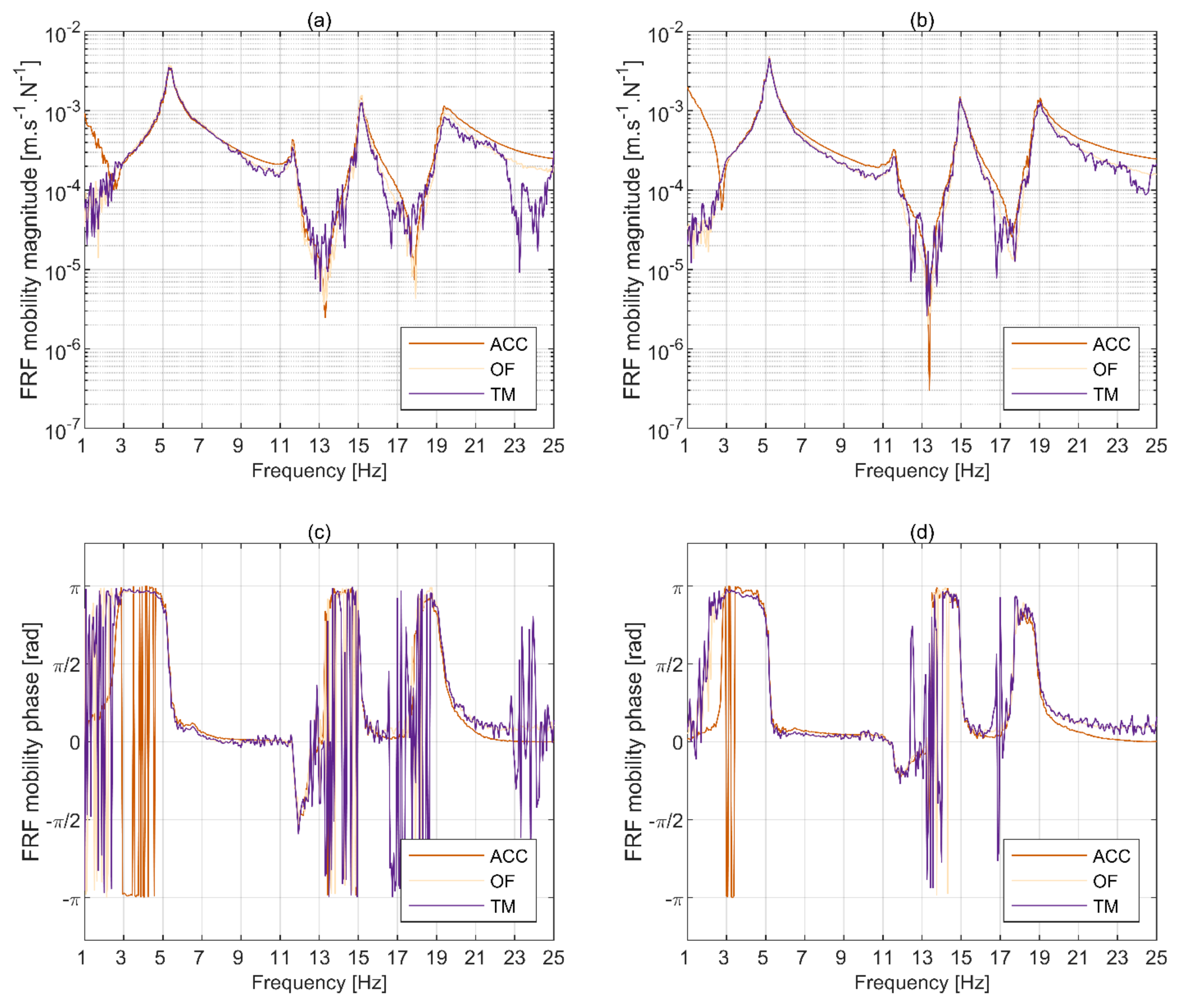
  • Optic flow algorithm consistently gives better results than template matching.
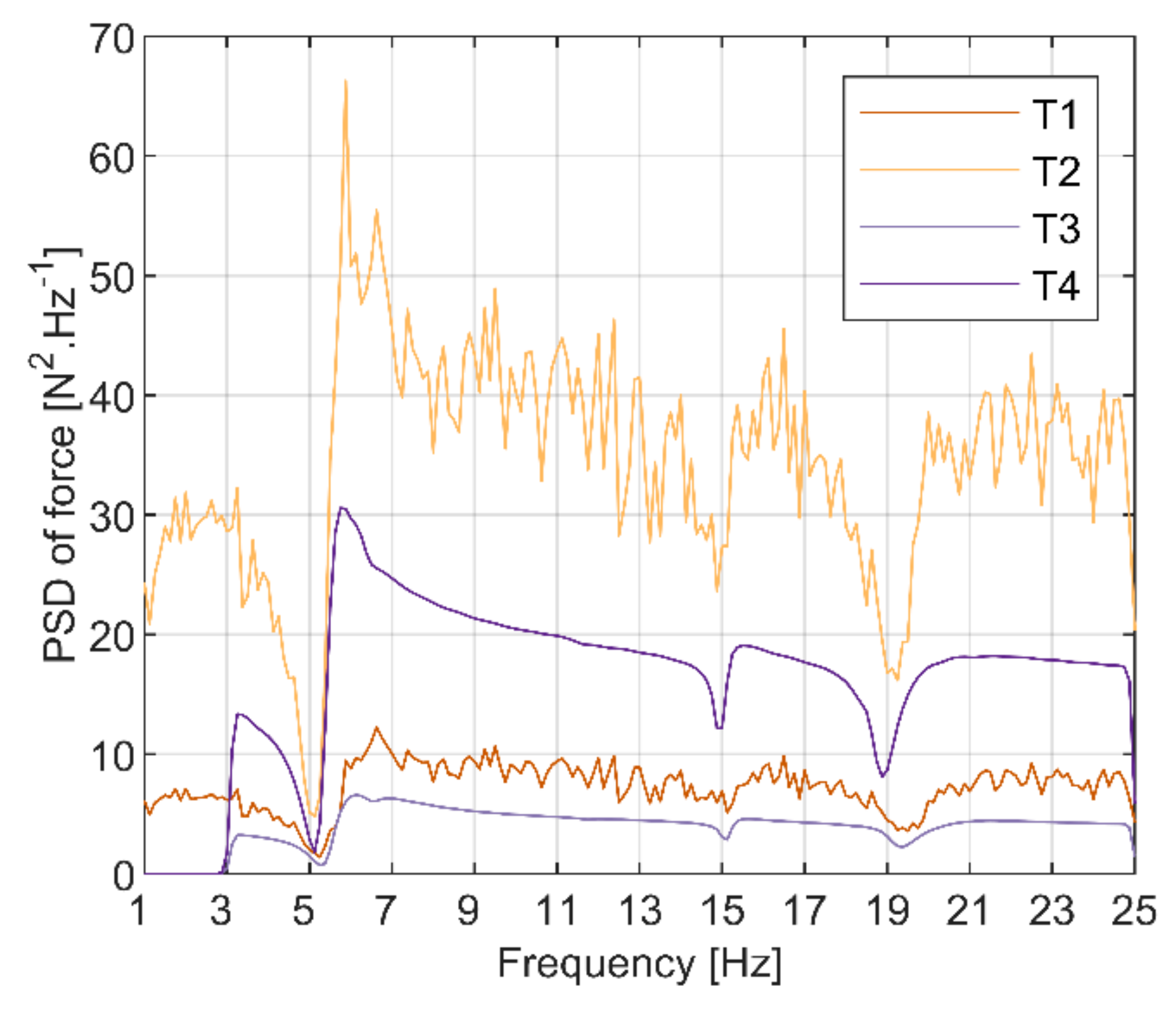
  • Relative to the benchmark results obtained with accelerometry, the pseudo random excitation gives superior results to sine chirp excitation regardless of the excitation intensity.
  • The error in modal parameters derived from optical MCS relative to accelerometry is within the uncertainty bounds imposed by the excitation type and intensity when considering the identification results from accelerometry only.
  • The necessary processing of images by the motion extraction algorithms unavoidably generates noise, the nature of which appears to be random. To alleviate this effect, the duration of the test should be long enough to be able to average out the noise while preserving sufficient frequency resolution. This also applies in the case of sine chirp excitation, which, in theory, should not require windowing and averaging due to the periodicity of the excitation signal.
  • Although in the case of shaker excitation, a H2 estimator is sometimes preferred to define resonances [62] (p. 288), the noise associated with the extraction of motion data from images overwrites this casualty making a H1 estimator more suitable for obtaining FRFs.
  • As is often the case in modal analysis, the modal parameters are sensitive to the data processing method, e.g., the length of blocks of data. This is also the case when using optical MCS, and suitable stabilisation diagrams can be used to gain confidence in the reliability of the results.
Overall, the results of this study encourage wider utilisation of camera-based vibration monitoring systems in engineering practice and motivate efforts to fully exploit the high-end information (i.e., by deriving modal damping and mass), apart from the modal frequencies and mode shapes typically reported.

Author Contributions

Conceptualization, M.B.; methodology, M.K. and M.B.; software, M.K.; validation, M.B.; formal analysis, M.K. and M.B.; resources, M.B., W.P., J.G. and N.N.; data curation, M.K.; writing—original draft preparation, M.K., M.B., N.N., W.P. and J.G.; writing—review and editing, M.B. and N.N.; visualization, M.K. and M.B.; supervision, M.B. and N.N.; project administration, M.B.; funding acquisition, M.K., M.B. and N.N. All authors have read and agreed to the published version of the manuscript.

Funding

M.K. was supported by the Bolashak International Scholarship of the President of the Republic of Kazakhstan for doctoral studies at the University of Leicester, UK. M.B. was supported by the Polish National Agency for Academic Exchange (NAWA) under the Polish Returns programme, grant number PPN/PPO/2019/1/00036. N.N. was supported by the UK Collaboratorium for Research in Infrastructure & Cities (UKCRIC) and the Engineering and Physical Sciences Research Council (EPSRC) under capital grant number EP/P017169/1 (National Centre for Infrastructure Materials in Leeds).

Institutional Review Board Statement

Not applicable.

Informed Consent Statement

Not applicable.

Data Availability Statement

Data are available from M.K. upon request.

Acknowledgments

Władysław Czyryński of the Department of Roads, Bridges, Railways and Airports at Wrocław University of Science and Technology in Poland is acknowledged for providing assistance in laboratory work. Sumit S. Parale is acknowledged for providing assistance with the integration of OpenCV libraries.

Conflicts of Interest

The authors declare no conflict of interest.

References

  1. Feng, D.; Feng, M.Q. Computer Vision for Structural Dynamics and Health Monitoring; John Wiley & Sons and ASME Press: Hoboken, NJ, USA, 2020. [Google Scholar]
  2. Ye, X.W.; Dong, C.Z.; Liu, T. A Review of Machine Vision-Based Structural Health Monitoring: Methodologies and Applications. J. Sens. 2016, 2016, 7103039. [Google Scholar] [CrossRef] [Green Version]
  3. Baqersad, J.; Poozesh, P.; Niezrecki, C.; Avitabile, P. Photogrammetry and optical methods in structural dynamics—A review. Mech. Syst. Signal Process. 2017, 86, 17–34. [Google Scholar] [CrossRef]
  4. Feng, D.; Feng, M.Q. Computer vision for SHM of civil infrastructure: From dynamic response measurement to damage detection—A review. Eng. Struct. 2018, 156, 105–117. [Google Scholar] [CrossRef]
  5. Spencer, B.F.; Hoskere, V.; Narazaki, Y. Advances in Computer Vision-Based Civil Infrastructure Inspection and Monitoring. Engineering 2019, 5, 199–222. [Google Scholar] [CrossRef]
  6. Dong, C.-Z.; Catbas, F.N. A review of computer vision–based structural health monitoring at local and global levels. Struct. Health Monit. 2020, 1475921720935585. [Google Scholar] [CrossRef]
  7. Zona, A. Vision-based vibration monitoring of structures and infrastructures: An overview of recent applications. Infrastructures 2021, 6, 4. [Google Scholar] [CrossRef]
  8. Xu, Y.; Brownjohn, J.M.W. Review of machine-vision based methodologies for displacement measurement in civil structures. J. Civ. Struct. Health Monit. 2018, 8, 91–110. [Google Scholar] [CrossRef] [Green Version]
  9. Lydon, D.; Lydon, M.; Taylor, S.; Del Rincon, J.M.; Hester, D.; Brownjohn, J. Development and field testing of a vision-based displacement system using a low cost wireless action camera. Mech. Syst. Signal Process. 2019, 121, 343–358. [Google Scholar] [CrossRef] [Green Version]
  10. Brownjohn, J.M.W.; Hester, D.; Xu, Y.; Bassitt, J.; Koo, K. Viability of optical tracking systems for monitoring deformations of a long span bridge. In Proceedings of the 6th European Conference on structural Control, Sheffield, UK, 11–13 July 2016; pp. 11–13. [Google Scholar] [CrossRef]
  11. Zhao, X.; Ri, K.; Wang, N. Experimental Verification for Cable Force Estimation Using Handheld Shooting of Smartphones. J. Sens. 2017, 5625396. [Google Scholar] [CrossRef] [Green Version]
  12. Khuc, T.; Catbas, F.N. Completely contactless structural health monitoring of real-life structures using cameras and computer vision. Struct. Control Health Monit. 2017, 24, e1852. [Google Scholar] [CrossRef]
  13. Dong, C.Z.; Bas, S.; Catbas, F.N. Investigation of vibration serviceability of a footbridge using computer vision-based methods. Eng. Struct. 2020, 224, 111224. [Google Scholar] [CrossRef]
  14. Luo, L.; Feng, M.Q.; Wu, Z.Y. Robust vision sensor for multi-point displacement monitoring of bridges in the field. Eng. Struct. 2018, 163, 255–266. [Google Scholar] [CrossRef]
  15. Xu, Y.; Brownjohn, J.; Kong, D. A non-contact vision-based system for multipoint displacement monitoring in a cable-stayed footbridge. Struct. Control Health Monit. 2018, 25, 1–23. [Google Scholar] [CrossRef] [Green Version]
  16. Kromanis, R.; Xu, Y.; Lydon, D.; Martinez del Rincon, J.; Al-Habaibeh, A. Measuring structural deformations in the laboratory environment using smartphones. Front. Built Environ. 2019, 5, 44. [Google Scholar] [CrossRef] [Green Version]
  17. Kohut, P.; Holak, K.; Uhl, T.; Ortyl, Ł.; Owerko, T.; Kuras, P.; Kocierz, R. Monitoring of a civil structure’s state based on noncontact measurements. Struct. Health Monit. 2013, 12, 411–429. [Google Scholar] [CrossRef]
  18. Yang, Y.; Dorn, C.; Mancini, T.; Talken, Z.; Kenyon, G.; Farrar, C.; Mascareñas, D. Blind identification of full-field vibration modes from video measurements with phase-based video motion magnification. Mech. Syst. Signal Process. 2017, 85, 567–590. [Google Scholar] [CrossRef]
  19. Park, S.W.; Park, H.S.; Kim, J.H.; Adeli, H. 3D displacement measurement model for health monitoring of structures using a motion capture system. Meas. J. Int. Meas. Confed. 2015, 59, 352–362. [Google Scholar] [CrossRef]
  20. Park, H.S.; Young Kim, J.; Gi Kim, J.; Woon Choi, S.; Kim, Y. A new position measurement system using a motion-capture camera for wind tunnel tests. Sensors 2013, 13, 12329–12344. [Google Scholar] [CrossRef] [Green Version]
  21. Oh, B.K.; Hwang, J.W.; Kim, Y.; Cho, T.; Park, H.S. Vision-based system identification technique for building structures using a motion capture system. J. Sound Vib. 2015, 356, 72–85. [Google Scholar] [CrossRef]
  22. Dong, C.Z.; Celik, O.; Catbas, F.N. Marker-free monitoring of the grandstand structures and modal identification using computer vision methods. Struct. Health Monit. 2019, 18, 1491–1509. [Google Scholar] [CrossRef]
  23. Hoskere, V.; Park, J.W.; Yoon, H.; Spencer, B.F. Vision-Based Modal Survey of Civil Infrastructure Using Unmanned Aerial Vehicles. J. Struct. Eng. 2019, 145, 1–14. [Google Scholar] [CrossRef]
  24. Morgenthal, G.; Hallermann, N.; Kersten, J.; Taraben, J.; Debus, P.; Helmrich, M.; Rodehorst, V. Framework for automated UAS-based structural condition assessment of bridges. Autom. Constr. 2019, 97, 77–95. [Google Scholar] [CrossRef]
  25. Feng, D.; Feng, M.Q. Vision-based multipoint displacement measurement for structural health monitoring. Struct. Control Health Monit. 2016. [Google Scholar] [CrossRef]
  26. Feng, D.; Feng, M.Q. Experimental validation of cost-effective vision-based structural health monitoring. Mech. Syst. Signal Process. 2017, 88, 199–211. [Google Scholar] [CrossRef]
  27. Jamali, S.; Chan, T.H.T.; Nguyen, A.; Thambiratnam, D.P. Reliability-based load-carrying capacity assessment of bridges using structural health monitoring and nonlinear analysis. Struct. Health Monit. 2019, 18, 20–34. [Google Scholar] [CrossRef] [Green Version]
  28. Celik, O.; Dong, C.-Z.; Catbas, F.N. Computer Vision–Based Human Comfort Assessment of Stadiums. J. Perform. Constr. Facil. 2020, 34, 04020005. [Google Scholar] [CrossRef]
  29. Cha, Y.J.; Chen, J.G.; Büyüköztürk, O. Output-only computer vision based damage detection using phase-based optical flow and unscented Kalman filters. Eng. Struct. 2017, 132, 300–313. [Google Scholar] [CrossRef]
  30. Celik, O.; Dong, C.; Catbas, F.N. A computer vision approach for the load time history estimation of lively individuals and crowds. Comput. Struct. 2018, 200, 32–52. [Google Scholar] [CrossRef]
  31. Dan, D.; Ge, L.; Yan, X. Identification of moving loads based on the information fusion of weigh-in-motion system and multiple camera machine vision. Measurement 2019, 144, 155–166. [Google Scholar] [CrossRef]
  32. Tian, Y.; Zhang, J.; Yu, S. Rapid Impact Testing and System Identification of Footbridges Using Particle Image Velocimetry. Comput. Civ. Infrastruct. Eng. 2019, 34, 130–145. [Google Scholar] [CrossRef]
  33. Tian, Y.; Zhang, J.; Yu, S. Vision-based structural scaling factor and flexibility identification through mobile impact testing. Mech. Syst. Signal Process. 2019, 122, 387–402. [Google Scholar] [CrossRef]
  34. Wang, Y.; Brownjohn, J.; Dai, K.; Patel, M. An Estimation of Pedestrian Action on Footbridges Using Computer Vision Approaches. Front. Built Environ. 2019, 5, 1–11. [Google Scholar] [CrossRef] [Green Version]
  35. Xu, Y.; Brownjohn, J.M.W.; Huseynov, F. Accurate Deformation Monitoring on Bridge Structures Using a Cost-Effective Sensing System Combined with a Camera and Accelerometers: Case Study. J. Bridg. Eng. 2019, 24, 05018014. [Google Scholar] [CrossRef] [Green Version]
  36. Ozer, E.; Feng, D.; Feng, M.Q. Hybrid motion sensing and experimental modal analysis using collocated smartphone camera and accelerometers. Meas. Sci. Technol. 2017, 28, 105903. [Google Scholar] [CrossRef]
  37. Javh, J.; Slavič, J.; Boltežar, M. High frequency modal identification on noisy high-speed camera data. Mech. Syst. Signal Process. 2018, 98, 344–351. [Google Scholar] [CrossRef]
  38. Javh, J.; Slavič, J.; Boltežar, M. Experimental modal analysis on full-field DSLR camera footage using spectral optical flow imaging. J. Sound Vib. 2018, 434, 213–220. [Google Scholar] [CrossRef]
  39. Orlowitz, E.; Brandt, A. Comparison of experimental and operational modal analysis on a laboratory test plate. Measurement 2017, 102, 121–130. [Google Scholar] [CrossRef]
  40. Brincker, R.; Ventura, C.E. Introduction to Operational Modal Analysis; John Wiley & Sons: Chichester, UK, 2015; ISBN 9781118535141. [Google Scholar]
  41. Brandt, A.; Berardengo, M.; Manzoni, S.; Cigada, A. Scaling of mode shapes from operational modal analysis using harmonic forces. J. Sound Vib. 2017, 407, 128–143. [Google Scholar] [CrossRef]
  42. Aenlle, M.; Juul, M.; Brincker, R. Modal Mass and Length of Mode Shapes in Structural Dynamics. Shock Vib. 2020, 2020. [Google Scholar] [CrossRef]
  43. Scruton, C. Wind-excited oscillations of tall stacks. Engineering 1955, 199, 806–808. [Google Scholar]
  44. McRobie, A.; Morgenthal, G. Risk Management for Pedestrian-Induced Dynamics of Footbridges. In Proceedings of the Footbridge 2002—First International Conference, Paris, France, 20–22 November 2002; pp. 1–10. [Google Scholar]
  45. Bocian, M.; Macdonald, J.H.G.; Burn, J.F. Probabilistic criteria for lateral dynamic stability of bridges under crowd loading. Comput. Struct. 2014, 136, 108–119. [Google Scholar] [CrossRef]
  46. Kalybek, M.; Bocian, M.; Nikitas, N. Performance of optical structural vibration monitoring systems in experimental modal analysis. Sensors 2021, 21, 1239. [Google Scholar] [CrossRef] [PubMed]
  47. Brandt, A. Noise and Vibration Analysis: Signal Analysis and Experimental Procedures; John Wiley and Sons: Hoboken, NJ, USA, 2011; ISBN 9780470746448. [Google Scholar]
  48. Cao, M.S.; Sha, G.G.; Gao, Y.F.; Ostachowicz, W. Structural damage identification using damping: A compendium of uses and features. Smart Mater. Struct. 2017, 26, 043001. [Google Scholar] [CrossRef]
  49. Balmes, E. GARTEUR group on ground vibration testing. Results from the test of a single structure by 12 laboratories in Europe. Proc. Int. Modal Anal. Conf. IMAC 1997, 2, 1346–1352. [Google Scholar]
  50. Reu, P.L.; Rohe, D.P.; Jacobs, L.D. Comparison of DIC and LDV for practical vibration and modal measurements. Mech. Syst. Signal Process. 2017, 86, 2–16. [Google Scholar] [CrossRef] [Green Version]
  51. Dong, C.Z.; Bas, S.; Necati Catbas, F. A completely non-contact recognition system for bridge unit influence line using portable cameras and computer vision. Smart Struct. Syst. 2019, 24, 617–630. [Google Scholar] [CrossRef]
  52. Pakos, W.; Wójcicki, Z.; Grosel, J.; Majcher, K.; Sawicki, W. Experimental research of cable tension tuning of a scaled model of cable stayed bridge. Arch. Civ. Mech. Eng. 2016, 16, 41–52. [Google Scholar] [CrossRef]
  53. Avitabile, P. Modal Testing: A Practitioner’s Guide; Wiley: Hoboken, NJ, USA, 2017. [Google Scholar]
  54. Garrido-Jurado, S.; Muñoz-Salinas, R.; Madrid-Cuevas, F.J.; Marín-Jiménez, M.J. Automatic generation and detection of highly reliable fiducial markers under occlusion. Pattern Recognit. 2014, 47, 2280–2292. [Google Scholar] [CrossRef]
  55. Hartley, R.; Zisserman, A. Multiple View Geometry in Computer Vision; Cambridge University Press: Cambridge, UK, 2004. [Google Scholar]
  56. Pan, B.; Qian, K.; Xie, H.; Asundi, A. Two-dimensional digital image correlation for in-plane displacement and strain measurement: A review. Meas. Sci. Technol. 2009, 20, 062001. [Google Scholar] [CrossRef]
  57. Evangelidis, G.D.; Psarakis, E.Z. Parametric image alignment using enhanced correlation coefficient maximization. IEEE Trans. Pattern Anal. Mach. Intell. 2008, 30, 1858–1865. [Google Scholar] [CrossRef] [PubMed] [Green Version]
  58. Shi, J.; Tomasi, C. Good features to track. In Proceedings of the IEEE Computer Society Conference on Computer Vision and Pattern Recognition;IEEE Conference on Computer Vision and Pattern Recognition, Seattle, WA, USA, 21–23 June 1994; pp. 593–600. [Google Scholar]
  59. Lucas, B.D.; Kanade, T. An Iterative Image Registration Technique with an Application to Stereo Vision. Int. Jt. Conf. Artif. Intell. 1981, 2, 674–679. [Google Scholar]
  60. MATLAB. Available online: https://uk.mathworks.com/products/matlab.html (accessed on 31 August 2021).
  61. Ewins, D.J. Modal Testing: Theory, Practice and Application; Research Studies Press Ltd.: Baldock, Hertfordshire, UK, 2000. [Google Scholar]
  62. Bendat, J.S.; Piersol, A.G. Random Data: Analysis and Measurement Procedures, 4th ed.; John Wiley & Sons: New York, NY, USA, 2012; ISBN 9781118032428. [Google Scholar]
  63. Hester, D.; Koo, K.; Xu, Y.; Brownjohn, J.; Bocian, M. Boundary condition focused finite element model updating for bridges. Eng. Struct. 2019, 198, 109514. [Google Scholar] [CrossRef]
  64. Poozesh, P.; Sabato, A.; Sarrafi, A.; Niezrecki, C.; Avitabile, P.; Yarala, R. Multicamera measurement system to evaluate the dynamic response of utility-scale wind turbine blades. Wind Energy 2020, 23, 1619–1639. [Google Scholar] [CrossRef]
  65. Warren, C.; Niezrecki, C.; Avitabile, P.; Pingle, P. Comparison of FRF measurements and mode shapes determined using optically image based, laser, and accelerometer measurements. Mech. Syst. Signal Process. 2011, 25, 2191–2202. [Google Scholar] [CrossRef]
Figure 1. Outline of the data fusion undertaken to enable experimental modal analysis (EMA).
Remotesensing 13 03471 g001
Figure 2. Layout of the bridge model and instrumentation systems; (a) overview, (b) zomed-in section of the deck near the shaker attachment. All dimensions in mm. In modal analysis, the performance of the bridge model in XY plane only was of interest.
Remotesensing 13 03471 g002
Figure 3. Truncated time histories of (a) excitation force and (b) structural response at the point of application of force during T2 and T4.
Remotesensing 13 03471 g003
Figure 4. Optical motion capture system.
Remotesensing 13 03471 g004
Figure 5. Original and resampled acceleration measured at the excitation point during T2 in (a) time and (b) frequency domain and the corresponding plots for T4 in (c,d). Signals in (a,c) were filtered with a 4th order Butterworth filter with cut off frequencies of 3 & 23 Hz and 1 & 23 Hz, respectively. PSDs in (b,d) were obtained without averaging and windowing.
Remotesensing 13 03471 g005aRemotesensing 13 03471 g005b
Figure 6. Truncated time-aligned response signals recorded at the excitation point during (a) T2 and (b) T4.
Remotesensing 13 03471 g006
Figure 7. Imaginary part of driving point accelerance FRF from (a) T2 and (b) T4.
Remotesensing 13 03471 g007
Figure 8. Driving point mobility for T1 & T2, respectively, in terms of (a,b) magnitude and (c,d) phase, together with (e,f) magnitude-squared coherence. All signals were processed using 71 blocks of 16 s length with uniform window and 50% overlap, giving frequency resolution Δf = 0.0625 Hz.
Remotesensing 13 03471 g008
Figure 9. Driving point FRF mobility from sine chirp excitation in (a) T3 and (b) T4.
Remotesensing 13 03471 g009
Figure 10. Driving point mobility for T3 & T4, respectively, in terms of (a,b) magnitude and (c,d) phase, together with (e,f) magnitude-squared coherence. All signals were processed using 16 s length with uniform window and 50% overlap, giving frequency resolution Δf = 0.0625 Hz.
Remotesensing 13 03471 g010aRemotesensing 13 03471 g010b
Figure 11. Exemplar stabilisation plots for modal parameters derived for (a) mode 1, (b) mode 3 and (c) mode 4 from T2.
Remotesensing 13 03471 g011
Figure 12. Errors in modal parameters obtained with optical motion capture systems: (a) frequency, (b) damping, (c) mass.
Remotesensing 13 03471 g012aRemotesensing 13 03471 g012b
Figure 13. Partial mode shapes for T2: (a) mode 1, (b) mode 3 and (c) mode 4.
Remotesensing 13 03471 g013aRemotesensing 13 03471 g013b
Figure 14. Modal assurance criterion (MAC) for all tests.
Remotesensing 13 03471 g014
Figure 15. Power spectra density of the input force for all tests.
Remotesensing 13 03471 g015
Figure 16. Bearing’s arrangement.
Remotesensing 13 03471 g016
Figure 17. Errors in modal parameters obtained with accelerometry for tests T1, T3, and T4 in comparison to T2: (a) frequency, (b) damping, (c) mass.
Remotesensing 13 03471 g017aRemotesensing 13 03471 g017b
Table 1. Summary of the conducted modal tests.
Test IDExcitation TypeRate [Hz/s]Intensity
[RMS *, N]
Approximate Test Duration [s]Frequency Range [Hz]
T1pseudo-randomn/a13.356003–25
T2pseudo-randomn/a28.956003–25
T3sine chirp0.0379.696003–25
T4sine chirp0.03719.86003–25
* RMS = root-mean-square.
Table 2. Basic specification of the instrumentation systems used in this study.
SystemSensorQuantityOperational Frequency and Resolution/Range/Sensitivity
AccelerometryBrüel & Kjær miniature DeltaTron® 4507 B005100.4 Hz–6 kHz
150 µg & 100 mV/(m·s−2)
Vibration exciterBrüel & Kjær Type 480815 Hz–10 kHz *
112 N
Force transducerBrüel & Kjær DeltaTron® 8230-003122000 N (compression) & 2200 N (tension)
0.22 mV/N
Data acquisition systemBrüel & Kjær PULSE14096 Hz
24 bit
Consumer-grade camera (CGC)Canon EOS 200D with DIGIC 7 processor and 20 mm Canon lens with maximum aperture f/2.8159.94 fps
24.2 MP
* Although 5 Hz in the nominal lowest frequency at which the input force can be fully controlled, the shaker can deliver force below that frequency, as shown in Section 4.
Table 3. Modal properties. Values in brackets denote percentage error relative to the results from accelerometry.
Frequency (Hz)Damping Ratio (%)Generalised Mass (kg)
TestModeAccelerometryTMOFAccelerometryTMOFAccelerometryTMOF
T115.3845.373
(−0.2)
5.368
(−0.3)
4.795.00
(4.38)
4.97
(3.76)
89.583.7
(−6.45)
84.1
(−6.01)
T1315.21815.215
(−0.02)
15.213
(−0.03)
0.700.68
(−2.86)
0.71
(1.43)
353.0418.9
(18.67)
463.3
(31.24)
T1419.63719.634
(−0.02)
19.627
(−0.05)
1.911.88
(−1.57)
1.89
(−1.05)
79.8111.7
(39.91)
127.9
(60.24)
T215.1825.180
(−0.04)
5.177
(−0.1)
3.193.24
(1.57)
3.22
(0.94)
87.892.4
(5.2)
98.3
(11.85)
T2315.08215.081
(−0.01)
15.08
(−0.01)
0.780.76
(−2.56)
0.77
(−1.28)
371.9387.3
(4.14)
383.3
(3.06)
T2419.17819.183
(0.03)
19.18
(0.01)
2.092.06
(−1.44)
2.06
(−1.44)
80.7101.6
(25.97)
84.13
(4.3)
T315.3985.381
(−0.31)
5.368
(−0.56)
2.912.66
(−8.59)
2.82
(−3.09)
110.8112.5
(1.51)
103.8
(−6.34)
T3315.21015.143
(−0.44)
15.155
(−0.36)
0.880.46
(−47.73)
0.52
(−40.91)
369.7640.5
(73.22)
426.5
(15.35)
T3419.41019.499
(0.46)
19.326
(0.43)
1.151.70
(47.83)
0.70
(−39.13)
119.2104.5
(−12.36)
171.9
(44.2)
T415.1825.215
(0.64)
5.214
(0.62)
2.922.89
(−1.03)
2.79
(−4.45)
94.090.9
(−3.21)
96.2
(2.4)
T4315.05915.015
(−0.29)
15.053
(−0.04)
0.900.60
(−33.33)
0.72
(−20)
396.3466.2
(17.63)
469.6
(18.47)
T4418.96019.084
(0.65)
18.912
(−0.25)
1.071.43
(33.64)
0.71
(−33.64)
109.2134.0
(22.71)
182.2
(66.85)
Table 4. Modal assurance criterion (MAC) for all tests.
TestOptical MCSMode 1Mode 3Mode 4
T1Template matching (TM)0.96500.97630.9875
T1Optic flow (OF)0.99820.99860.9964
T2Template matching (TM)0.95130.99030.9931
T2Optic flow (OF)0.95280.99660.9928
T3Template matching (TM)0.99040.96170.9901
T3Optic flow (OF)0.99260.97590.9865
T4Template matching (TM)0.98660.97230.9921
T4Optic flow (OF)0.98700.98410.9962
Publisher’s Note: MDPI stays neutral with regard to jurisdictional claims in published maps and institutional affiliations.

